Abstract

In this paper, we explore the initial-boundary value (IBV) problem for an integrable spin-1 Gross-Pitaevskii system with a $4\times 4$ Lax pair on the finite interval $x\in[0,L]$ by extending the Fokas unified transform approach. The solution of this system can be expressed in terms of the solution of a $4\times 4$ matrix Riemann-Hilbert (RH) problem formulated in the complex $k$-plane. Furthermore, the relevant jump matrices with explicit $(x,t)$-dependence of the matrix RH problem can be explicitly found via three spectral functions $\{s(k),\,S(k),\,S_{L}(k)\}$ arising from the initial data and the Dirichlet-Neumann boundary conditions at $x=0$ and $x=L$, respectively. The global relation is also found to deduce two distinct but equivalent types of representations (i.e., one via the large $k$ of asymptotics of the eigenfunctions and another one in terms of the Gel’fand-Levitan-Marchenko (GLM) approach) for the Dirichlet and Neumann boundary value problems. In particular, the formulae for IBV problems on the finite interval can reduce to ones on a half-line as the length $L$ of the interval approaches to infinity. Moreover, we also present the linearizable boundary conditions for the GLM representations.

Keywords: Integrable spin-1 Gross-Pitaevskii system; Initial-boundary value problem; Riemann-Hilbert problem; Global relation; Finite interval; GLM representation; Maps between Dirichlet and Neumann problems

Mathematics Subject Classification numbers: 37K15; 35Q15; 34A55

1 Introduction

At the end of the 1960s, the well-known inverse scattering transform (IST) [1] (also called nonlinear Fourier transform) was first presented to solve the initial value problem for the KdV equation starting from its two linear eigenvalue equations (also called the Lax pair [2]). After that, the IST was used to solve many integrable nonlinear evolution equations (NLEEs) with Lax pairs (see, e.g., Ref. [3, 4] and references therein), in which the initial conditions were usually chosen as the constants or plane waves to generate bright or dark solitons and breathers. In the early 1990s, Deift and Zhou [5] developed the IST method to present the powerful nonlinear steepest descent method to analytically study the long-time asymptotics of the Cauchy problems of the (1+1)-dimensional integrable NLEEs such as the mKdV equation and nonlinear Schrödinger equation. At the end of the 1990s, Fokas [6] further extended the idea of the IST to present a unified method studying initial-boundary value problems for both linear and nonlinear integrable equations with Lax pairs (see Refs. [7, 8, 9, 10, 11, 12] for the details). Particularly, the Fokas method is used to study integrable nonlinear PDEs by means of the simultaneous spectral analysis of both parts of the Lax pairs and the global relation among the spectral functions. This differs from the classical IST, in which the spectral analysis of only one part of the Lax pairs was considered. The Fokas method well unites the key ideas of the IST with the Riemann-Hilbert problems [9, 11].

The Fokas method, as a novel and effective method, has been used to study the initial-boundary value (IBV) problems for the linear PDEs and some integrable NLEEs with $2\times 2$ Lax pairs on the half-line and the finite interval such as, the nonlinear Schrödinger (NLS) equation [6, 13, 15, 16, 14], the sine-Gordon equation [17, 18], the KdV equation [19, 20], the modified KdV equation [21, 23, 22, 24], the derivative NLS equation [25], and etc. (see, e.g., Refs. [26, 27, 28, 11, 29, 30, 31] and references therein). Recently, Lenells further developed the Fokas method to analyze the IBV problems for integrable NLEEs with $3\times 3$ Lax pairs on the half-line [32]. After that, the modified approach was applied in the IBV problems of other integrable NLEEs with $3\times 3$ Lax pairs on the half-line or the finite interval, such as the Degasperis-Procesi equation [33], the Sasa-Satsuma equation [34], the coupled NLS equations [35, 36, 37], and the Ostrovsky-Vakhnenko equation [38].

More recently, we [39] successfully extended the ideas of the Fokas method [6] for the $2\times 2$ Lax pairs and its extension [32] for the $3\times 3$ Lax pairs to study the IBV problems for the integrable spin-1 GP system [40, 41, 42] with a $4\times 4$ Lax pair on the half-line $0<x<\infty$

$$\left\{\begin{array}[]{l}\displaystyle i\frac{\partial q_{1}}{\partial t}+\frac{\partial^{2}q_{1}}{\partial x^{2}}-2\alpha\left(|q_{1}|^{2}+2|q_{0}|^{2}\right)q_{1}-2\alpha\beta q_{0}^{2}\bar{q}_{-1}=0,\vspace{0.1in}\\ \displaystyle i\frac{\partial q_{0}}{\partial t}+\frac{\partial^{2}q_{0}}{\partial x^{2}}-2\alpha\left(|q_{1}|^{2}+|q_{0}|^{2}+|q_{-1}|^{2}\right)q_{0}-2\alpha\beta q_{1}q_{-1}\bar{q}_{0}=0,\vspace{0.1in}\\ \displaystyle i\frac{\partial q_{-1}}{\partial t}+\frac{\partial^{2}q_{-1}}{\partial x^{2}}-2\alpha\left(2|q_{0}|^{2}+|q_{-1}|^{2}\right)q_{-1}-2\alpha\beta q_{0}^{2}\bar{q}_{1}=0,\end{array}\right.\quad\alpha^{2}=\beta^{2}=1,$$ (4)

with the IBV conditions

$$\left\{\!\!\!\begin{array}[]{lll}{\rm Initial\,\,conditions:}&q_{j}(x,t=0)=q_{0j}(x),&\!j=1,0,-1,\quad 0<x<\infty,\vspace{0.1in}\\ {\rm Dirichlet\,\,boundary\,\,conditions:}&q_{j}(x=0,t)=u_{0j}(t),&\!j=1,0,-1,\quad 0<t<\infty,\vspace{0.1in}\\ {\rm Neumann\,\,boundary\,\,conditions:}&q_{jx}(x=0,t)=u_{1j}(t),&\!j=1,0,-1,\quad 0<t<\infty,\end{array}\right.$$ (8)

where the overbar stands for the complex conjugate. The spin-1 GP system (4) can describe soliton dynamics of an $F=1$ spinor Bose-Einstein condensates [40]. The four types of parameters: $(\alpha,\beta)=\{(1,1),(1,-1),(-1,1),(-1,-1)\}$ in the spin-1 GP system (4) correspond to the four roles of the self-cross-phase modulation (nonlinearity) and spin-exchange modulation, respectively, that is, (attractive, attractive), (attractive, repulsive), (repulsive, attractive), and (repulsive, repulsive).

In this paper, we extend the idea in Ref. [39] from the half-line to the finite interval $0<x<L<\infty$. The aim of this paper is to develop a methodology for analyzing the integrable spin-1 GP system (4) with the following IBV problem

$$\left\{\begin{array}[]{lll}\!\!\!{\rm Initial\,\,data:}&\!\!q_{j}(x,t=0)=q_{0j}(x),&0<x<L,\vspace{0.1in}\\ \!\!\!{\rm Dirichlet\,\,boundary\,\,data:}&\!\!q_{j}(x=0,t)=u_{0j}(t),&q_{j}(x=L,t)=v_{0j}(t),\,\,0<t<T,\vspace{0.1in}\\ \!\!\!{\rm Neumann\,\,boundary\,\,data:}&q_{jx}(x=0,t)=u_{1j}(t),&q_{jx}(x=L,t)=v_{1j}(t),\,\,0<t<T,\end{array}\right.$$ (12)

$j=1,0,-1$, on the finite interval

$$\Omega=\left\{(x,t)\,|\,x\in[0,L],\,t\in[0,T]\right\}$$ (13)

with $L>0$ and $T>0$ being the fixed finite length and time, respectively, the initial data $q_{0j}(x),\,j=1,0,-1$ and boundary data $\{u_{0j}(t),\,u_{1j}(t),\,j=1,0,-1\}$ are sufficiently smooth and compatible at points $(x,t)=(0,0)$. where the initial data $q_{0j}(x),\,j=1,0,-1$ and boundary data $\{u_{sj}(t),\,v_{sj}(t),\,s=0,1;\,j=1,0,-1\}$ are sufficiently smooth and compatible at points $(x,t)=(0,0),\,(L,0)$, respectively.

The main steps for analyzing the IBV problem for the integrable spin-1 GP system (4) with Eq. (12) are listed as follows:

Step 1. Suppose that a sufficiently smooth solution $\{q_{j}(x,t),\,j=1,0,-1\},\,0<x<L,\,0<t<T$ of the integrable spin-1 GP system (4) exists, we implement the direct spectral analysis of the corresponding Lax pair in order to explore these points:

• Introduce appropriate solutions of the exact one-form of the modified Lax pair (32), which are bounded and analytic for the isospectral parameter $k$ in domains to form a partition of the Riemann sphere.

• Introduce the following matrix-valued spectral functions

  • $s(k)$ is determined using the initial data $q_{j}(x,0)=q_{0j}(x),\,j=1,0,-1,\,0<x<L$;

  • $S(k)$ is generated using the boundary data at $x=0$, $q_{j}(x=0,t)=u_{0j}(t),\,q_{jx}(x=0,t)=u_{1j}(t),\,j=1,0,-1,\,0<t<T$;

  • $S_{L}(k)$ is determined using the boundary data at $x=L$, $q_{j}(x=L,t)=v_{0j}(t),\,q_{jx}(x=L,t)=v_{1j}(t),\,j=1,0,-1,\,0<t<T$;

• Show that these above-mentioned spectral functions satisfy a global relation, which implies that the initial-boundary value conditions can not be chosen arbitrary.

Step 2. Use the spectral functions $\{s(k),\,S(k),\,S_{L}(k)\}$ to determine a regular Reimann-Hilbert problem, whose solution can generate a solution of the spin-1 GP system (4).

Step 3. The Gel’fand-Levitan-Marchenko (GLM) representations can also given for the IBV problem of system (4).

The rest of this paper is organized as follows. In Sec. 2, we introduce the $4\times 4$ Lax pair of Eq. (4) and explore its spectral analysis such as the eigenfunctions, the jump matrices, and the global relation. Sec. 3 exhibits the corresponding $4\times 4$ matrix RH problem in terms of the jump matrices found in Sec. 2. The global relation is found to generate the map between the Dirichlet and Neumann boundary values in Sec. 4. Particularly, the relevant formulae for boundary value problems on the finite interval can reduce to ones on the half-line as the length of the interval approaches to infinity. In Sec. 5, we give the GLM representations of the eigenfunctions in terms of the global relation. Moreover, we also show that the GLM representations are equivalent to ones in Sec. 4 and present the linearizable boundary conditions for the GLM representations. Finally, we give the conclusions and discussions.

2 A $4\times 4$ Lax pair and its spectral analysis

2.1.  The closed one-form

The integrable spin-1 GP system (4) can be regarded as a compatibility condition of the following $4\times 4$ Lax pair formulation [40, 39]

$$\left\{\begin{array}[]{l}\psi_{x}+ik\sigma_{4}\psi=U(x,t)\psi,\vspace{0.1in}\\ \psi_{t}+2ik^{2}\sigma_{4}\psi=V(x,t,k)\psi,\end{array}\right.$$ (16)

where $\psi\equiv\psi(x,t,k)$ is a $4\times 1$ column vector-valued or 4$\times$4 matrix-valued eigenfunction, $k\in\mathbb{C}$ is an iso-spectral parameter, $\sigma_{4}={\rm diag}(1,1,-1,-1)$, and the $4\times 4$ matrix-valued functions $U(x,t)$ and $V(x,t,k)$ are given as

$$U(x,t)=\left(\begin{array}[]{cccc}0&0&q_{1}(x,t)&q_{0}(x,t)\vspace{0.05in}\\ 0&0&\beta q_{0}(x,t)&q_{-1}(x,t)\vspace{0.05in}\\ \alpha\bar{q}_{1}(x,t)&\alpha\beta\bar{q}_{0}(x,t)&0&0\vspace{0.05in}\\ \alpha\bar{q}_{0}(x,t)&\alpha\bar{q}_{-1}(x,t)&0&0\end{array}\right),\quad\bar{U}^{T}(x,t)=\alpha U(x,t),$$ (21)

and

$$\begin{array}[]{l}V(x,t,k)=2kU+i\sigma_{4}(U_{x}-U^{2})\vspace{0.1in}\\ \quad=\left(\begin{array}[]{cccc}-i\alpha(|q_{1}|^{2}+|q_{0}|^{2})&-i\alpha(\beta q_{1}\bar{q}_{0}+q_{0}\bar{q}_{-1})&iq_{1x}+2kq_{1}&iq_{0x}+2kq_{0}\vspace{0.1in}\\ -i\alpha(\beta q_{0}\bar{q}_{1}+q_{-1}\bar{q}_{0})&-i\alpha(|q_{-1}|^{2}+|q_{0}|^{2})&\beta(iq_{0x}+2kq_{0})&iq_{-1x}+2kq_{-1}\vspace{0.1in}\\ \alpha(-i\bar{q}_{1x}+2k\bar{q}_{1})&\alpha\beta(-i\bar{q}_{0x}+2k\bar{q}_{0})&i\alpha(|q_{1}|^{2}+|q_{0}|^{2})&i\alpha(\beta q_{-1}\bar{q}_{0}+q_{0}\bar{q}_{1})\vspace{0.1in}\\ \alpha(-i\bar{q}_{0x}+2k\bar{q}_{0})&\alpha(-i\bar{q}_{-1x}+2k\bar{q}_{-1})&i\alpha(\beta q_{0}\bar{q}_{-1}+q_{1}\bar{q}_{0})&i\alpha(|q_{-1}|^{2}+|q_{0}|^{2})\end{array}\right).\end{array}$$ (28)

where the potential function $\{q_{j}(x,t),\,j=1,0,-1\}$ satisfies the spin-1 GP equations (4).

Introduce a new eigenfunction $\mu(x,t,k)$ defined by

$$\mu(x,t,k)=\psi(x,t,k)e^{i(kx+2k^{2}t)\sigma_{4}},$$ (29)

such that the Lax pair (16) becomes an equivalent form

$$\left\{\begin{array}[]{l}\mu_{x}+ik[\sigma_{4},\mu]=U(x,t)\mu,\vspace{0.1in}\\ \mu_{t}+2ik^{2}[\sigma_{4},\mu]=V(x,t,k)\mu,\end{array}\right.$$ (32)

where $[\sigma_{4},\mu]\equiv\sigma_{4}\mu-\mu\sigma_{4}$.

Let $\hat{\sigma}_{4}$ denote the commutator with respect to $\sigma_{4}$ and the operator acting on a $4\times 4$ matrix $A$ by $\hat{\sigma}_{4}A=[\sigma_{4},A]=\sigma_{4}A-A\sigma_{4}$ such that $e^{\hat{\sigma}_{4}}A=e^{\sigma_{4}}Ae^{-\sigma_{4}}$, then the Lax pair (32) can be written as a full derivative form

$$d\left[e^{i(kx+2k^{2}t)\hat{\sigma}_{4}}\mu(x,t,k)\right]=W(x,t,k),$$ (33)

where $W(x,t,k)$ is the exact one-form defined by

$$W(x,t,k)=e^{i(kx+2k^{2}t)\hat{\sigma}_{4}}\left[U(x,t)\mu(x,t,k)dx+V(x,t,k)\mu(x,t,k)dt\right].$$ (34)

Notice that Eq. (33) can be used to obtain an expression for $\mu(x,t,k)$ via the fundamental theorem of calculus.

2.2.   The eigenfunctions $\{\mu_{j}(x,t,k)\}_{1}^{4}$

For any point $(x,t)\in\Omega=\{(x,t)|x\in[0,L],\,t\in[0,T]\}$, we assume that $\{\gamma_{j}\}_{1}^{4}$ denote the four contours connecting fours vertexes

$$(x_{1},t_{1})=(0,T),\quad(x_{2},t_{2})=(0,0),\quad(x_{3},t_{3})=(L,0),\quad(x_{4},t_{4})=(L,T),$$

of the rectangle $\Omega$ to the point $(x,t)$ (see Fig. 1). Thus for any point $(\xi,\tau)\in\gamma_{j},\,j=1,2,3,4$, we have the relations on the contours:

$$\begin{array}[]{rll}\gamma_{1}:&x-\xi\geq 0,&t-\tau\leq 0,\vspace{0.1in}\\ \gamma_{2}:&x-\xi\geq 0,&t-\tau\geq 0,\vspace{0.1in}\\ \gamma_{3}=-\gamma_{1}:&x-\xi\leq 0,&t-\tau\geq 0,\vspace{0.1in}\\ \gamma_{4}=-\gamma_{2}:&x-\xi\leq 0,&t-\tau\leq 0,\end{array}$$ (39)

where the negative sign in $\gamma_{3}=-\gamma_{1}$ and $\gamma_{4}=-\gamma_{2}$ denotes the opposite directions.

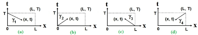
Figure 1: The contours $\gamma_{j}\,(j=1,2,3,4)$ exhibited in the finite region $\Omega=\{(x,t)|x\in[0,L],\,t\in[0,T]\}$.

We assume that system (4) possesses a smooth complex-valued solution $\{q_{j}(x,t),\,j=1,0,-1\}$ in the domain $\Omega$ (if $T=\infty$ then we assume that the solution $\{q_{j}(x,t),\,j=1,0,-1\}$ is a sufficient decay as $t\to\infty$). It follows from the Lax pair (32) that we can define its four eigenfunctions (sectionally holomorphic functions) $\{\mu_{j}(x,t,k)\}_{1}^{4}$ on the four contours $\{\gamma_{j}\}_{1}^{4}$

$$\begin{array}[]{rl}\mu_{j}(x,t,k)=&\!\!\!\displaystyle\mathbb{I}+\int_{\gamma_{j}}e^{-i(kx+2k^{2}t)\hat{\sigma}_{4}}W_{j}(\xi,\tau,k)\vspace{0.1in}\\ =&\!\!\!\displaystyle\mathbb{I}+\int_{(x_{j},t_{j})}^{(x,t)}e^{-i(kx+2k^{2}t)\hat{\sigma}_{4}}W_{j}(\xi,\tau,k),\quad j=1,2,3,4.\end{array}$$ (42)

in terms of the Volterra integral equations, where $\mathbb{I}={\rm diag}(1,1,1,1)$, the integral is over a piecewise smooth curve from $(x_{j},t_{j})$ to $(x,t)$, $W_{j}(x,t,k)$’s are defined by Eq. (34) with $\mu(x,t,k)$ replaced by $\mu_{j}(x,t,k)$’s. Since the one-forms $W_{j}(x,t,k)$’s are closed, thus $\mu_{j}(x,t,k)$’s are independent of the path of integration. The integral Eq. (42) reduces to

$$\begin{array}[]{rl}\mu_{j}(x,t,k)=&\displaystyle\mathbb{I}+\int_{x_{j}}^{x}e^{-ik(x-\xi)\hat{\sigma}_{4}}(U\mu_{j})(\xi,t,k)d\xi\vspace{0.1in}\\ &\displaystyle+e^{-ik(x-x_{j})\hat{\sigma}_{4}}\int_{t_{j}}^{t}e^{-2ik^{2}(t-\tau)\hat{\sigma}_{4}}(V\mu_{j})(x_{j},\tau,k)d\tau,\quad j=1,2,3,4.\end{array}$$ (45)

if the paths of integration are chosen to be parallel to the $x$ and $t$ axes.

Eq. (45) implies that the four columns of the matrix $\mu_{j}(x,t,k)$ contain, respectively, these exponentials

$$\quad[\mu_{j}(x,t,k)]_{s}:\,\,e^{2i[k(x-\xi)+2k^{2}(t-\tau)]},\quad e^{2i[k(x-\xi)+2k^{2}(t-\tau)]},\quad s=1,2;j=1,2,3,4,\vspace{0.1in}$$ (46a)

$$\qquad[\mu_{j}(x,t,k)]_{s}:\,\,e^{-2i[k(x-\xi)+2k^{2}(t-\tau)]},\quad e^{-2i[k(x-\xi)+2k^{2}(t-\tau)]},\quad s=3,4;j=1,2,3,4,$$ (46b)

To analyze the bounded regions of the eigenfunctions $\{\mu_{j}(x,t,k)\}_{1}^{4}$, we need to use the curve

$$K=\{k\in\mathbb{C}|({\rm Re}\,f(k))({\rm Re}\,g(k))=0,\,f(k)=ik,\,g(k)=ik^{2}\},$$

to separate the complex $k$-plane into four domains (see Fig. 2):

$$\left\{\begin{array}[]{l}D_{1}=\{k\in\mathbb{C}\,|\,{\rm Re}\,f(k)<0\,\,{\rm and}\,\,{\rm Re}\,g(k)<0\},\vspace{0.1in}\\ D_{2}=\{k\in\mathbb{C}\,|\,{\rm Re}\,f(k)<0\,\,{\rm and}\,\,{\rm Re}\,g(k)>0\},\vspace{0.1in}\\ D_{3}=\{k\in\mathbb{C}\,|\,{\rm Re}\,f(k)>0\,\,{\rm and}\,\,{\rm Re}\,g(k)<0\},\vspace{0.1in}\\ D_{4}=\{k\in\mathbb{C}\,|\,{\rm Re}\,f(k)>0\,\,{\rm and}\,\,{\rm Re}\,g(k)>0\},\end{array}\right.$$ (51)

which imply that $D_{1}$ and $D_{3}$ ($D_{2}$ and $D_{4}$) are symmetric about the origin of the complex $k$-plane.

Therefore, it follows from Eqs. (39), (46) and (51) that the regions, where the distinct columns of eigenfunctions $\{\mu_{j}(x,t,k)\}_{1}^{4}$ are bounded and analytic in the complex $k$-plane, are given below:

$$\left\{\begin{array}[]{l}\mu_{1}(x,t,k):(f_{-}\cap g_{+},\,f_{-}\cap g_{+},\,f_{+}\cap g_{-},\,f_{+}\cap g_{-})=:(D_{2},D_{2},D_{3},D_{3}),\vspace{0.1in}\\ \mu_{2}(x,t,k):(f_{-}\cap g_{-},\,f_{-}\cap g_{-},\,f_{+}\cap g_{+},\,f_{+}\cap g_{+})=:(D_{1},D_{1},D_{4},D_{4}),\vspace{0.1in}\\ \mu_{3}(x,t,k):(f_{+}\cap g_{-},\,f_{+}\cap g_{-},\,f_{-}\cap g_{+},\,f_{-}\cap g_{+})=:(D_{3},D_{3},D_{2},D_{2}),\vspace{0.1in}\\ \mu_{4}(x,t,k):(f_{+}\cap g_{+},\,f_{+}\cap g_{+},\,f_{-}\cap g_{-},\,f_{-}\cap g_{-})=:(D_{4},D_{4},D_{1},D_{1}),\end{array}\right.$$ (56)

where $f_{+}=:{\rm Re}\,f(k)>0,\,f_{-}=:{\rm Re}\,f(k)<0,\,g_{+}=:{\rm Re}\,g(k)>0$, and $g_{-}=:{\rm Re}\,g(k)<0$.

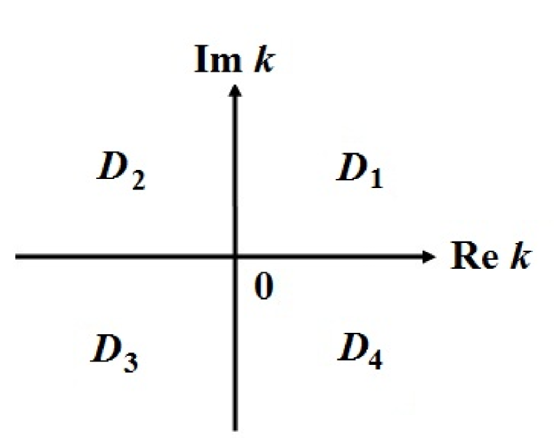
Figure 2: The regions $D_{n},\,(n=1,2,3,4)$ separating the complex $k$-plane.

2.3.   The new matrix-valued functions $M_{n}(x,t,k)$’s

We introduce the matrix-valued solutions $M_{n}(x,t,k),\,n=1,2,3,4$ of Eq. (32) in the form

$$(M_{n})_{lj}(x,t,k)=\delta_{lj}+\int_{(\gamma^{n})_{lj}}\left[e^{-i(kx+2k^{2}t)\hat{\sigma}_{4}}W_{n}(\xi,\tau,k)\right]_{lj},\quad l,j=1,2,3,4,\quad k\in D_{n},$$ (57)

via the Volterra integral equations, where $\delta_{ij}=1$ for $l=j$ and $\delta_{ij}=0$ for $l\not=j$, $W_{n}(x,t,k)$ is defined by

$$W_{n}(x,t,k)=e^{i(kx+2k^{2}t)\hat{\sigma}_{4}}\left[U(x,t)M_{n}(x,t,k)dx+V(x,t,k)M_{n}(x,t,k)dt\right].$$ (58)

and the contours $(\gamma^{n})_{lj}$’s are defined as

$$(\gamma^{n})_{lj}=\left\{\begin{array}[]{l}\gamma_{1},\,\,\,{\rm if}\,\,{\rm Re}\,f_{l}(k)<{\rm Re}\,f_{j}(k)\,\,{\rm and}\,\,{\rm Re}\,g_{l}(k)\geq{\rm Re}\,g_{j}(k),\vspace{0.1in}\\ \gamma_{2},\,\,\,{\rm if}\,\,{\rm Re}\,f_{l}(k)<{\rm Re}\,f_{j}(k)\,\,{\rm and}\,\,{\rm Re}\,g_{l}(k)<{\rm Re}\,g_{j}(k),\vspace{0.1in}\\ \gamma_{3},\,\,\,{\rm if}\,\,{\rm Re}\,f_{l}(k)\geq{\rm Re}\,f_{j}(k)\,\,{\rm and}\,\,{\rm Re}\,g_{l}(k)\leq{\rm Re}\,g_{j}(k),\vspace{0.1in}\\ \gamma_{4},\,\,\,{\rm if}\,\,{\rm Re}\,f_{l}(k)\geq{\rm Re}\,f_{j}(k)\,\,{\rm and}\,\,{\rm Re}\,g_{l}(k)\geq{\rm Re}\,g_{j}(k),\end{array}\right.\quad k\in D_{n},\quad l,j=1,2,3,4,$$ (63)

where $f_{1,2}(k)=-f_{3,4}(k)=-ik$ and $g_{1,2}(k)=-g_{3,4}(k)=-2ik^{2}$.

Remark. To distinguish $(\gamma^{n})_{lj}$’s to be the contour $\gamma_{3}$ or $\gamma_{4}$ for the special cases, ${\rm Re}\,f_{l}(k)={\rm Re}\,f_{j}(k)$ and ${\rm Re}\,g_{l}(k)={\rm Re}\,g_{j}(k)$, we choose them as $\gamma_{3}$ (or $\gamma_{4})$ in these cases if we can determine that $\gamma_{3}$ (or $\gamma_{4})$ must appear in other positions of the matrices $\gamma^{n}$.

The definition (63) of $(\gamma^{n})_{lj}$ can generate the explicit expressions of $\gamma^{n}\,(n=1,2,3,4)$ as

$$\begin{array}[]{rr}\gamma^{1}=\left(\begin{array}[]{cccc}\gamma_{4}&\gamma_{4}&\gamma_{4}&\gamma_{4}\\ \gamma_{4}&\gamma_{4}&\gamma_{4}&\gamma_{4}\\ \gamma_{2}&\gamma_{2}&\gamma_{4}&\gamma_{4}\\ \gamma_{2}&\gamma_{2}&\gamma_{4}&\gamma_{4}\end{array}\right),&\gamma^{2}=\left(\begin{array}[]{cccc}\gamma_{3}&\gamma_{3}&\gamma_{3}&\gamma_{3}\\ \gamma_{3}&\gamma_{3}&\gamma_{3}&\gamma_{3}\\ \gamma_{1}&\gamma_{1}&\gamma_{3}&\gamma_{3}\\ \gamma_{1}&\gamma_{1}&\gamma_{3}&\gamma_{3}\end{array}\right),\vspace{0.1in}\\ \gamma^{3}=(\gamma^{2})^{T}=\left(\begin{array}[]{cccc}\gamma_{3}&\gamma_{3}&\gamma_{1}&\gamma_{1}\\ \gamma_{3}&\gamma_{3}&\gamma_{1}&\gamma_{1}\\ \gamma_{3}&\gamma_{3}&\gamma_{3}&\gamma_{3}\\ \gamma_{3}&\gamma_{3}&\gamma_{3}&\gamma_{3}\end{array}\right),&\gamma^{4}=(\gamma^{1})^{T}=\left(\begin{array}[]{cccc}\gamma_{4}&\gamma_{4}&\gamma_{2}&\gamma_{2}\\ \gamma_{4}&\gamma_{4}&\gamma_{2}&\gamma_{2}\\ \gamma_{4}&\gamma_{4}&\gamma_{4}&\gamma_{4}\\ \gamma_{4}&\gamma_{4}&\gamma_{4}&\gamma_{4}\end{array}\right),\end{array}$$ (82)

Proposition 2.1. For the matrix-valued functions $M_{n}(x,t,k),\,n=1,2,3,4$ defined by Eq. (57) for $k\in\bar{D}_{n}$ and $(x,t)\in\Omega$ and any fixed point $(x_{0},t_{0})$, $M_{n}(x_{0},t_{0},k)$’s are the bounded and analytic function of $k\in D_{n}$ away from a possible discrete set of singularity $\{k_{j}\}$ at which the Fredholm determinants vanish. Furthermore, $M_{n}(x,t,k)$’s also have the bounded and continuous extensions to $\bar{D}_{n}$ and

$$M_{n}(x,t,k)=\mathbb{I}+O\left(\frac{1}{k}\right),\,\,k\in D_{n},\,\,n=1,2,3,4,\,\ k\to\infty,$$ (83)

Proof. Following the proof for the $3\times 3$ Lax pair in Ref. [32], we can also show the bounedness and analyticity of the $4\times 4$ matrix $M_{n}(x,t,k)$. The substitution of the eigenfunction

$$\mu(x,t,k)=M_{n}(x,t,k)=M_{n}^{(0)}(x,t)+\sum_{j=1}^{\infty}\frac{M_{n}^{(j)}(x,t)}{k^{j}},\quad k\to\infty,\,\,n=1,2,3,4,$$

into the $x$-part of the Lax pair (32) can obtain Eq. (83). $\square$

Notice that the above-defined functions $M_{n}(x,t,k)$’s can be used to formulate a $4\times 4$ matrix Riemann-Hilbert problem.

2.4.   The minors of eigenfunctions and Lax pair

The cofactor matrix $X^{A}$ (or the transpose of the adjugate) of a $4\times 4$ matrix $X$ is given by

$${\rm adj}(X)^{T}=X^{A}=\left(\begin{array}[]{rrrr}m_{11}(X)&-m_{12}(X)&m_{13}(X)&-m_{14}(X)\vspace{0.05in}\\ -m_{21}(X)&m_{22}(X)&-m_{23}(X)&m_{24}(X)\vspace{0.05in}\\ m_{31}(X)&-m_{32}(X)&m_{33}(X)&-m_{34}(X)\vspace{0.05in}\\ -m_{41}(X)&m_{42}(X)&-m_{43}(X)&m_{44}(X)\end{array}\right),$$ (88)

where $m_{ij}(X)$ denotes the $(ij)$th minor of $X$, and $(X^{A})^{T}X={\rm adj}(X)X=\det X$.

It follows from the Lax pair (32) that the cofactor matrices $\{\mu_{j}^{A}(x,t,k)\}_{1}^{4}$ of the matrices $\{\mu_{j}(x,t,k)\}_{1}^{4}$ satisfy the modified Lax equation

$$\left\{\begin{array}[]{l}\mu_{j,x}^{A}(x,t,k)-ik\hat{\sigma}_{4}\mu_{j}^{A}(x,t,k)=-U^{T}(x,t)\mu_{j}^{A}(x,t,k),\vspace{0.1in}\\ \mu_{j,t}^{A}(x,t,k)-2ik^{2}\hat{\sigma}_{4}\mu_{j}^{A}(x,t,k)=-V^{T}(x,t,k)\mu_{j}^{A}(x,t,k),\end{array}\right.$$ (91)

whose solutions can also be expressed as

$$\begin{array}[]{rl}\mu_{j}^{A}(x,t,k)=&\!\!\!\mathbb{I}-\displaystyle\int_{\gamma_{j}}e^{i[k(x-\xi)+2k^{2}(t-\tau)]\hat{\sigma}_{4}}\left[U^{T}(\xi,\tau)d\xi+V^{T}(\xi,\tau,k)d\tau\right]\mu_{j}^{A}(\xi,\tau,k)\vspace{0.1in}\\ =&\!\!\!\displaystyle\mathbb{I}-\int_{x_{j}}^{x}e^{ik(x-\xi)\hat{\sigma}_{4}}(U^{T}\mu_{j}^{A})(\xi,t,k)d\xi\vspace{0.1in}\\ &\quad\displaystyle-e^{ik(x-x_{j})\hat{\sigma}_{4}}\int_{t_{j}}^{t}e^{2ik^{2}(t-\tau)\hat{\sigma}_{4}}(V^{T}\mu_{j}^{A})(x_{j},\tau,k)d\tau,\quad j=1,2,3,4\end{array}$$ (95)

using the Volterra integral equations, where $U^{T}(x,t,k)$ and $V^{T}(x,t,k)$ denote the transposes of $U(x,t,k)$ and $V(x,t,k)$ given by Eq. (21), respectively.

Therefore, the regions of boundedness of $\mu_{j}^{A}(x,t,k),\,j=1,2,3,4$ are given by

$$\left\{\begin{array}[]{l}\mu_{1}^{A}(x,t,k){\rm\,\,is\,\,bounded\,\,for\,\,}k\in(D_{3},D_{3},D_{2},D_{2}),\vspace{0.1in}\\ \mu_{2}^{A}(x,t,k){\rm\,\,is\,\,bounded\,\,for\,\,}k\in(D_{4},D_{4},D_{1},D_{1}),\vspace{0.1in}\\ \mu_{3}^{A}(x,t,k){\rm\,\,is\,\,bounded\,\,for\,\,}k\in(D_{2},D_{2},D_{3},D_{3}),\vspace{0.1in}\\ \mu_{4}^{A}(x,t,k){\rm\,\,is\,\,bounded\,\,for\,\,}k\in(D_{1},D_{1},D_{4},D_{4}),\end{array}\right.$$ (100)

which are symmetric ones of $\mu_{j}$ about the ${\rm Re}\,k$-axis (cf. Eq. (56)).

2.5.  Symmetries of eigenfunctions

Let

$$\check{U}(x,t,k)=-ik\sigma_{4}+U(x,t,k),\quad\check{V}(x,t,k)=-2ik^{2}\sigma_{4}+V(x,t,k).$$ (101)

Since

$$P_{\pm}\overline{\check{U}(x,t,\bar{k})}P_{\pm}=-\check{U}(x,t,k)^{T},\quad P_{\pm}\overline{\check{V}(x,t,\bar{k})}P_{\pm}=-\check{V}(x,t,k)^{T},$$ (102)

where

$$P_{\pm}=\left(\begin{array}[]{cccc}\pm\alpha&0&0&0\\ 0&\pm\alpha&0&0\\ 0&0&\mp 1&0\\ 0&0&0&\mp 1\end{array}\right),\quad P_{\pm}^{2}=\mathbb{I},\quad\alpha^{2}=1$$ (107)

According to Eq. (91), we have the following proposition:

Proposition 2.2. The eigenfunction $\psi(x,t,k)$ of the Lax pair (16) and $\mu_{j}(x,t,k)$ of the Lax pair (32) both possess the same symmetric relation

$$\begin{array}[]{l}\psi^{-1}(x,t,k)=P_{\pm}\overline{\psi(x,t,\bar{k})}^{T}P_{\pm},\vspace{0.1in}\\ \mu_{j}^{-1}(x,t,k)=P_{\pm}\overline{\mu_{j}(x,t,\bar{k})}^{T}P_{\pm},\quad j=1,2,3,4,\end{array}$$ (110)

Moreover, in the domains where $\mu_{j}$ is bounded, we have

$$\mu_{j}(x,t,k)=\mathbb{I}+O\left(\frac{1}{k}\right),\quad k\to\infty,\quad j=1,2,3,4$$

and

$${\rm det}[\mu_{j}(x,t,k)]=1,\quad j=1,2,3,4$$

since the traces of the matrices $U(x,t)$ and $V(x,t,k)$ are zero.

2.6.   The spectral functions

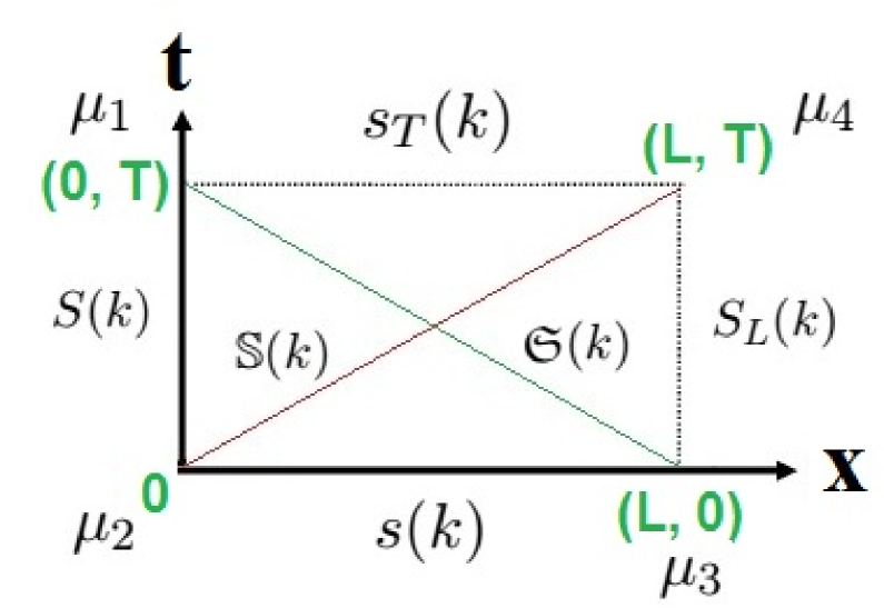
Figure 3: The relations among $\mu_{j}(x,t,k),\,j=1,2,3,4$.

Since $\mu_{j}(x,t,k)$ are linearly dependent, thus we can have six relations $\{S(k),s(k),\mathbb{S}(k),S_{L}(k),s_{T}(k),\mathfrak{S}(k)\}$ between any two eigenfunctions $\mu_{j}$ (see Fig. 3), however, we know that these six relations are not dependent such that we only introduce three of those, that is, the three $4\times 4$ matrix-valued functions $S(k),\,s(k)$ and $\mathbb{S}(k)$ between $\mu_{j}(x,t,k),\,j=1,3,4$ and $\mu_{2}(x,t,k)$ as

$$\begin{array}[]{l}\mu_{1}(x,t,k)=\mu_{2}(x,t,k)e^{-i(kx+2k^{2}t)\hat{\sigma}_{4}}S(k),\vspace{0.1in}\\ \mu_{3}(x,t,k)=\mu_{2}(x,t,k)e^{-i(kx+2k^{2}t)\hat{\sigma}_{4}}s(k),\vspace{0.1in}\\ \mu_{4}(x,t,k)=\mu_{2}(x,t,k)e^{-i(kx+2k^{2}t)\hat{\sigma}_{4}}\mathbb{S}(k),\end{array}$$ (114)

Evaluating system (114) at $(x,t)=(0,0)$ and the three equations in system (114) at $(x,t)=(0,T),(L,0),(L,T)$, respectively, we find

$$\begin{array}[]{l}S(k)=\mu_{1}(0,0,k)=e^{2ik^{2}T\hat{\sigma}_{4}}\mu_{2}^{-1}(0,T,k),\vspace{0.1in}\\ s(k)=\mu_{3}(0,0,k)=e^{ikL\hat{\sigma}_{4}}\mu_{2}^{-1}(L,0,k),\vspace{0.1in}\\ \mathbb{S}(k)=\mu_{4}(L,0,k)=e^{2ik^{2}T\hat{\sigma}_{4}}\mu_{3}^{-1}(L,T,k),\end{array}$$ (118)

It follows from Eqs. (114) and (118) that we can find the relations among $\{S(k),s(k),\mathbb{S}(k),S_{L}(k),s_{T}(k),\mathfrak{S}(k)\}$:

• the relation between $\mu_{3}(x,t,k)$ and $\mu_{1}(x,t,k)$

  $$\begin{array}[]{rl}\mu_{3}(x,t,k)=&\!\!\!\mu_{1}(x,t,k)e^{-i(kx+2k^{2}t)\hat{\sigma}_{4}}\mathfrak{S}(k),\end{array}$$ (120)

  with

  $$\mathfrak{S}(k)=S^{-1}(k)s(k),$$ (121)

  which generates the relation of the three edges of the triangle consisting of $(x_{j},t_{j}),\,j=1,2,3$.

• the relation between $\mu_{4}(x,t,k)$ and $\mu_{3}(x,t,k)$

  $$\begin{array}[]{rl}\mu_{4}(x,t,k)=&\!\!\!\mu_{3}(x,t,k)e^{-i[k(x-L)+2k^{2}(t-T)]\hat{\sigma}_{4}}\mu_{3}^{-1}(L,T,k)\vspace{0.1in}\\ =&\!\!\!\mu_{3}(x,t,k)e^{-i(kx+2k^{2}t)\hat{\sigma}_{4}}[s^{-1}(k)\mathbb{S}(k)]\vspace{0.1in}\\ =&\!\!\!\mu_{3}(x,t,k)e^{-i[k(x-L)+2k^{2}t]\hat{\sigma}_{4}}S_{L}(k),\end{array}$$ (125)

  with

  $$S_{L}(k)=\mu_{4}(L,0,k)=e^{2ik^{2}T\hat{\sigma}_{4}}\mu_{3}^{-1}(L,T,k)=e^{-ikL\hat{\sigma}_{4}}[s^{-1}(k)\mathbb{S}(k)],$$ (126)

  that is,

  $$\mathbb{S}(k)=s(k)e^{ikL\hat{\sigma}_{4}}S_{L}(k),$$ (127)

  which generates the relation of the three edges of the triangle consisting of $(x_{j},t_{j}),\,j=2,3,4$.

• the relation between $\mu_{1}(x,t,k)$ and $\mu_{4}(x,t,k)$

  $$\begin{array}[]{rl}\mu_{4}(x,t,k)=&\!\!\!\mu_{1}(x,t,k)e^{-i(kx+2k^{2}t)\hat{\sigma}_{4}}s_{T}(k),\end{array}$$ (129)

  with

  $$s_{T}(k)=S^{-1}(k)\mathbb{S}(k)=\mathfrak{S}(k)e^{ikL\hat{\sigma}_{4}}S_{L}(k)=S^{-1}(k)s(k)e^{ikL\hat{\sigma}_{4}}S_{L}(k),$$ (130)

which generates the relations of the three edges of the triangle consisting of $(x_{j},t_{j}),\,j=1,2,4$, of the three edges of the triangle consisting of $(x_{j},t_{j}),\,j=1,3,4$, and of the four edges of the rectangle consisting of $(x_{j},t_{j}),\,j=1,2,3,4$, respectively.

According to the definition (45) of $\mu_{j}$ and Eqs. (118) and (126), we have

$$\begin{array}[]{rl}S(k)=&\!\!\!\displaystyle\mathbb{I}-\int_{0}^{T}e^{2ik^{2}\tau\hat{\sigma}_{4}}(V\mu_{1})(0,\tau,k)d\xi=\left[\mathbb{I}+\int_{0}^{T}e^{2ik^{2}\tau\hat{\sigma}_{4}}(V\mu_{2})(0,\tau,k)d\tau\right]^{-1},\vspace{0.1in}\\ s(k)=&\!\!\!\displaystyle\mathbb{I}-\int_{0}^{L}e^{ik\xi\hat{\sigma}_{4}}(U\mu_{3})(\xi,0,k)d\xi=\left[\mathbb{I}+\int_{0}^{L}e^{ik\xi\hat{\sigma}_{4}}(U\mu_{2})(\xi,0,k)d\xi\right]^{-1},\vspace{0.1in}\\ S_{L}(k)=&\!\!\!\displaystyle\mathbb{I}-\int_{0}^{T}e^{2ik^{2}\tau\hat{\sigma}_{4}}(V\mu_{4})(L,\tau,k)d\tau=\left[\mathbb{I}+\int_{0}^{T}e^{2ik^{2}\tau\hat{\sigma}_{4}}(V\mu_{3})(L,\tau,k)d\tau\right]^{-1},\vspace{0.1in}\\ \end{array}$$ (134)

$$\begin{array}[]{rl}\mathbb{S}(k)=&\!\!\!\displaystyle\mathbb{I}-\int_{0}^{L}e^{ik\xi\hat{\sigma}_{4}}(U\mu_{4})(\xi,0,k)d\xi-e^{ikL\hat{\sigma}_{4}}\int_{0}^{T}e^{2ik^{2}\tau\hat{\sigma}_{4}}(V\mu_{4})(L,\tau,k)d\tau\vspace{0.1in}\\ =&\!\!\!\displaystyle\left[\mathbb{I}+e^{2ik^{2}T\hat{\sigma}_{4}}\int_{0}^{L}e^{ik\xi\hat{\sigma}_{4}}(U\mu_{2})(\xi,T,k)d\xi+\int_{0}^{T}e^{2ik^{2}\tau\hat{\sigma}_{4}}(V\mu_{2})(0,\tau,k)d\tau\right]^{-1}\vspace{0.1in}\\ =&\!\!\!\displaystyle\left[\mathbb{I}-\int_{0}^{L}e^{ik\xi\hat{\sigma}_{4}}(U\mu_{3})(\xi,0,k)d\xi\right]e^{ikL\hat{\sigma}_{4}}\left[\mathbb{I}-\int_{0}^{T}e^{2ik^{2}\tau\hat{\sigma}_{4}}(V\mu_{4})(L,\tau,k)d\tau\right]\vspace{0.1in}\\ =&\!\!\!\displaystyle\left[\mathbb{I}+\int_{0}^{L}e^{ik\xi\hat{\sigma}_{4}}(U\mu_{2})(\xi,0,k)d\xi\right]^{-1}e^{ikL\hat{\sigma}_{4}}\left[\mathbb{I}+\int_{0}^{T}e^{2ik^{2}\tau\hat{\sigma}_{4}}(V\mu_{3})(L,\tau,k)d\tau\right]^{-1},\vspace{0.1in}\\ \end{array}$$ (139)

$$\begin{array}[]{rl}\mathfrak{S}(k)=&\!\!\!\displaystyle\left[\mathbb{I}-\int_{0}^{T}e^{2ik^{2}\tau\hat{\sigma}_{4}}(V\mu_{1})(0,\tau,k)d\xi\right]^{-1}\left[\mathbb{I}-\int_{0}^{L}e^{ik\xi\hat{\sigma}_{4}}(U\mu_{3})(\xi,0,k)d\xi\right]\vspace{0.1in}\\ =&\!\!\!\displaystyle\left[\mathbb{I}+\int_{0}^{T}e^{2ik^{2}\tau\hat{\sigma}_{4}}(V\mu_{2})(0,\tau,k)d\tau\right]\left[\mathbb{I}+\int_{0}^{L}e^{ik\xi\hat{\sigma}_{4}}(U\mu_{2})(\xi,0,k)d\xi\right]^{-1},\vspace{0.1in}\\ \end{array}$$ (142)

$$\begin{array}[]{rl}s_{T}(k)=&\!\!\!\displaystyle\left[\mathbb{I}-\int_{0}^{T}e^{2ik^{2}\tau\hat{\sigma}_{4}}(V\mu_{1})(0,\tau,k)d\xi\right]^{-1}\left[\mathbb{I}-\int_{0}^{L}e^{ik\xi\hat{\sigma}_{4}}(U\mu_{3})(\xi,0,k)d\xi\right]\vspace{0.1in}\\ &\!\!\!\displaystyle\times e^{ikL\hat{\sigma}_{4}}\left[\mathbb{I}-\int_{0}^{T}e^{2ik^{2}\tau\hat{\sigma}_{4}}(V\mu_{4})(L,\tau,k)d\tau\right],\end{array}$$ (145)

where $\mu_{j_{2}}(0,t,k),\ j_{2}=1,2,\,\mu_{j_{3}}(L,t,k),\,j_{3}=3,4,\,\mu_{j_{1}}(x,0,k),\,j_{1}=2,3,4,\,0<x<L,\,0<t<T$ satisfy the integral equations

$$\begin{array}[]{l}\mu_{j}(0,t,k)=\displaystyle\mathbb{I}+\int_{T}^{t}e^{-2ik^{2}(t-\tau)\hat{\sigma}_{4}}(V\mu_{j})(0,\tau,k)d\tau,\quad j=1,2,\vspace{0.1in}\\ \mu_{j}(L,t,k)=\displaystyle\mathbb{I}+\int_{0}^{t}e^{-2ik^{2}(t-\tau)\hat{\sigma}_{4}}(V\mu_{j})(L,\tau,k)d\tau,\quad j=3,4,\vspace{0.1in}\\ \mu_{j}(x,0,k)=\displaystyle\mathbb{I}+\int_{0}^{x}e^{ik\xi\hat{\sigma}_{4}}(U\mu_{j})(\xi,0,k)d\xi,\quad j=2,3,\vspace{0.1in}\\ \mu_{4}(x,0,k)=\displaystyle\mathbb{I}+\int_{L}^{x}e^{ik\xi\hat{\sigma}_{4}}(U\mu_{4})(\xi,0,k)d\xi-e^{-ik(x-L)\hat{\sigma}_{4}}\int_{0}^{T}e^{2ik^{2}\tau\hat{\sigma}_{4}}(V\mu_{4})(L,\tau,k)d\tau.\end{array}$$ (150)

It follows from Eqs. (118) and (134) that $s(k),\,S(k)$ and $S_{L}(k)$ are determined by $U(x,0,k),\,V(0,t,k)$, and $V(L,t,k)$, that is, $s(k)$ is decided by the initial data $q_{j}(x,t=0)$, and $S(k)$ and $S_{L}(k)$ are found by the Dirichlet-Neumann boundary data $q_{j}(x,t)$ and $q_{jx}(x,t),\,j=1,0,-1$ at $x=0$ and $x=L$, respectively. In fact, $\mu_{3}(x,0,k)$ and $\{\mu_{1}(0,t,k),\,\mu_{4}(L,t,k)\}$ satisfy the $x$-part and $t$-part of the Lax pair (32) at $t=0$ and $x=0,L$, respectively, that is,

$$x-{\rm part}:\,\left\{\begin{array}[]{l}\mu_{x}(x,0,k)+ik\hat{\sigma}_{4}\mu(x,0,k)=U(x,t=0)\mu(x,0,k),\quad 0<x<L,\vspace{0.1in}\\ \displaystyle\mu(L,0,k)=\mathbb{I},\end{array}\right.$$ (153)

$$t-{\rm part}:\,\left\{\begin{array}[]{l}\mu_{t}(x_{j},t,k)+2ik^{2}\hat{\sigma}\mu(x_{j},t,k)=V(x=0,t,k)\mu(x-j,t,k),\,\,0<t<T,\,j=1,4,\vspace{0.1in}\\ \mu(x_{j},0,k)=\mathbb{I},\quad\mu(x_{j},T,k)=\mathbb{I},\quad x_{1}=0,\,x_{4}=L,\end{array}\right.$$ (156)

It follows from the properties of $\mu_{j}$ and $\mu_{j}^{A}$ that the functions $\{S(k),\,s(k),\,\mathbb{S}(k),\,S_{L}(k),\mathfrak{S}(k),\,s_{T}(k)\}$ and $\{S^{A}(k),\,s^{A}(k),\,\mathbb{S}^{A}(k),\,S_{L}^{A}(k),\,\mathfrak{S}^{A}(k),\,s_{T}^{A}(k)\}$ have the following boundedness:

$$\left\{\begin{array}[]{l}S(k){\rm\,\,is\,\,bounded\,\,for\,\,}k\in(D_{2}\cup D_{4},D_{2}\cup D_{4},D_{1}\cup D_{3},D_{1}\cup D_{3}),\vspace{0.1in}\\ s(k){\rm\,\,is\,\,bounded\,\,for\,\,}k\in(D_{3}\cup D_{4},D_{3}\cup D_{4},D_{1}\cup D_{2},D_{1}\cup D_{2}),\vspace{0.1in}\\ \mathbb{S}(k){\rm\,\,is\,\,bounded\,\,for\,\,}k\in(D_{4},D_{4},D_{1},D_{1}),\vspace{0.1in}\\ S_{L}(k){\rm\,\,is\,\,bounded\,\,for\,\,}k\in(D_{2}\cup D_{4},D_{2}\cup D_{4},D_{1}\cup D_{3},D_{1}\cup D_{3}),\vspace{0.1in}\\ \mathfrak{S}(k){\rm\,\,is\,\,bounded\,\,for\,\,}k\in(D_{4},D_{4},D_{1},D_{1}),\vspace{0.1in}\\ s_{T}(k){\rm\,\,is\,\,bounded\,\,for\,\,}k\in(D_{4},D_{4},D_{1},D_{1}),\vspace{0.1in}\\ \end{array}\right.$$ (163)

and

$$\left\{\begin{array}[]{l}S^{A}(k){\rm\,\,is\,\,bounded\,\,for\,\,}k\in(D_{1}\cup D_{3},D_{1}\cup D_{3},D_{2}\cup D_{4},D_{2}1\cup D_{4}),\vspace{0.1in}\\ s^{A}(k){\rm\,\,is\,\,bounded\,\,for\,\,}k\in(D_{1}\cup D_{2},D_{1}\cup D_{2},D_{3}\cup D_{4},D_{3}\cup D_{4}),\vspace{0.1in}\\ \mathbb{S}^{A}(k){\rm\,\,is\,\,bounded\,\,for\,\,}k\in(D_{2},D_{2},D_{3},D_{3}),\vspace{0.1in}\\ S_{L}^{A}(k){\rm\,\,is\,\,bounded\,\,for\,\,}k\in(D_{2}\cup D_{4},D_{2}\cup D_{4},D_{1}\cup D_{3},D_{1}\cup D_{3}),\vspace{0.1in}\\ \mathfrak{S}^{A}(k){\rm\,\,is\,\,bounded\,\,for\,\,}k\in(D_{2},D_{2},D_{3},D_{3}),\vspace{0.1in}\\ s_{T}^{A}(k){\rm\,\,is\,\,bounded\,\,for\,\,}k\in(D_{2},D_{2},D_{3},D_{3}),\end{array}\right.$$ (170)

Proposition 2.3. The new matrix-valued functions $S_{n}(k)=(S_{n}^{ij}(k))_{4\times 4},\,n=1,2,3,4$ introduced by

$$M_{n}(x,t,k)=\mu_{2}(x,t,k)e^{-i(kx+2k^{2}t)\hat{\sigma}_{4}}S_{n}(k),\quad k\in D_{n},$$ (171)

can be found uing the entries of the matrix-valued spectral functions $s(k)=(s_{ij}(k))_{4\times 4},\,S(k)=(S_{ij}(k))_{4\times 4}$, and $\mathbb{S}(k)=(\mathbb{S}_{ij}(k))_{4\times 4}=s(k)e^{ikL\hat{\sigma}_{4}}S_{L}(k)$ given by Eq. (118) as follows:

$$\begin{array}[]{ll}S_{1}(k)=\left(\begin{array}[]{cccc}\dfrac{m_{22}(\mathbb{S}(k))}{n_{33,44}(\mathbb{S}(k))}&\dfrac{m_{21}(\mathbb{S}(k))}{n_{33,44}(\mathbb{S}(k))}&\mathbb{S}_{13}(k)&\mathbb{S}_{14}(k)\vspace{0.1in}\\ \dfrac{m_{12}(\mathbb{S}(k))}{n_{33,44}(\mathbb{S}(k))}&\dfrac{m_{11}(\mathbb{S}(k))}{n_{33,44}(\mathbb{S}(k))}&\mathbb{S}_{23}(k)&\mathbb{S}_{24}(k)\vspace{0.1in}\\ 0&0&\mathbb{S}_{33}(k)&\mathbb{S}_{34}(k)\vspace{0.1in}\\ 0&0&\mathbb{S}_{43}(k)&\mathbb{S}_{44}(k)\end{array}\right),\vspace{0.15in}\\ S_{2}(k)=\left(\begin{array}[]{cccc}S_{2}^{11}(k)&S_{2}^{12}(k)&s_{13}(k)&s_{14}(k)\vspace{0.1in}\\ S_{2}^{21}(k)&S_{2}^{22}(k)&s_{23}(k)&s_{24}(k)\vspace{0.1in}\\ S_{2}^{31}(k)&S_{2}^{32}(k)&s_{33}(k)&s_{34}(k)\vspace{0.1in}\\ S_{2}^{41}(k)&S_{2}^{42}(k)&s_{43}(k)&s_{44}(k)\end{array}\right),\vspace{0.15in}\\ S_{3}(k)=\left(\begin{array}[]{cccc}s_{11}(k)&s_{12}(k)&S_{3}^{13}(k)&S_{3}^{14}(k)\vspace{0.1in}\\ s_{21}(k)&s_{22}(k)&S_{3}^{23}(k)&S_{3}^{24}(k)\vspace{0.1in}\\ s_{31}(k)&s_{32}(k)&S_{3}^{33}(k)&S_{3}^{34}(k)\vspace{0.1in}\\ s_{41}(k)&s_{42}(k)&S_{3}^{43}(k)&S_{3}^{44}(k)\end{array}\right),\vspace{0.15in}\\ S_{4}(k)=\left(\begin{array}[]{cccc}\mathbb{S}_{11}(k)&\mathbb{S}_{12}(k)&0&0\vspace{0.1in}\\ \mathbb{S}_{21}(k)&\mathbb{S}_{22}(k)&0&0\vspace{0.1in}\\ \mathbb{S}_{31}(k)&\mathbb{S}_{32}(k)&\dfrac{m_{44}(\mathbb{S}(k))}{n_{11,22}(\mathbb{S}(k))}&\dfrac{m_{43}(\mathbb{S}(k))}{n_{11,22}(\mathbb{S}(k))}\vspace{0.1in}\\ \mathbb{S}_{41}(k)&\mathbb{S}_{42}(k)&\dfrac{m_{34}(\mathbb{S}(k))}{n_{11,22}(\mathbb{S}(k))}&\dfrac{m_{33}(\mathbb{S}(k))}{n_{11,22}(\mathbb{S}(k))}\end{array}\right),\end{array}$$ (192)

where $n_{i_{1}j_{1},i_{2}j_{2}}(X)$ denotes the determinant of the sub-matrix generated by choosing the cross elements of $i_{1,2}$th rows and $j_{1,2}$th columns of a $4\times 4$ matrix $X$, that is,

$$n_{i_{1}j_{1},i_{2}j_{2}}(X)=\left|\begin{array}[]{cc}X_{i_{1}j_{1}}&X_{i_{1}j_{2}}\vspace{0.1in}\\ X_{i_{2}j_{1}}&X_{i_{2}j_{2}}\end{array}\right|.$$ (195)

and

$$\left\{\begin{array}[]{l}S_{2}^{1j}(k)=\dfrac{n_{1j,2(3-j)}(S)m_{2(3-j)}(s)+n_{1j,3(3-j)}(S)m_{3(3-j)}(s)+n_{1j,4(3-j)}(S)m_{4(3-j)}(s)}{\mathcal{N}([S]_{1}[S]_{2}[s]_{3}[s]_{4})},\vspace{0.1in}\\ S_{2}^{2j}(k)=\dfrac{n_{2j,1(3-j)}(S)m_{1(3-j)}(s)+n_{2j,3(3-j)}(S)m_{3(3-j)}(s)+n_{2j,4(3-j)}(S)m_{4(3-j)}(s)}{\mathcal{N}([S]_{1}[S]_{2}[s]_{3}[s]_{4})},\vspace{0.1in}\\ S_{2}^{3j}(k)=\dfrac{n_{3j,1(3-j)}(S)m_{1(3-j)}(s)+n_{3j,2(3-j)}(S)m_{2(3-j)}(s)+n_{3j,4(3-j)}(S)m_{4(3-j)}(s)}{\mathcal{N}([S]_{1}[S]_{2}[s]_{3}[s]_{4})},\vspace{0.1in}\\ S_{2}^{4j}(k)=\dfrac{n_{4j,1(3-j)}(S)m_{1(3-j)}(s)+n_{4j,2(3-j)}(S)m_{2(3-j)}(s)+n_{4j,3(3-j)}(S)m_{3(3-j)}(s)}{\mathcal{N}([S]_{1}[S]_{2}[s]_{3}[s]_{4})},\end{array}\right.\quad j=1,2,$$ (200)

$$\left\{\begin{array}[]{l}S_{3}^{1j}(k)=\dfrac{n_{1j,2(7-j)}(S)m_{2(7-j)}(s)+n_{1j,3(7-j)}(S)m_{3(7-j)}(s)+n_{1j,4(7-j)}(S)m_{4(7-j)}(s)}{\mathcal{N}([s]_{1}[s]_{2}[S]_{3}[S]_{4})},\vspace{0.1in}\\ S_{3}^{2j}(k)=\dfrac{n_{2j,1(7-j)}(S)m_{1(7-j)}(s)+n_{2j,3(7-j)}(S)m_{3(7-j)}(s)+n_{2j,4(7-j)}(S)m_{4(7-j)}(s)}{\mathcal{N}([s]_{1}[s]_{2}[S]_{3}[S]_{4})},\vspace{0.1in}\\ S_{3}^{3j}(k)=\dfrac{n_{3j,1(7-j)}(S)m_{1(7-j)}(s)+n_{3j,2(7-j)}(S)m_{2(7-j)}(s)+n_{3j,4(7-j)}(S)m_{4(7-j)}(s)}{\mathcal{N}([s]_{1}[s]_{2}[S]_{3}[S]_{4})},\vspace{0.1in}\\ S_{3}^{4j}(k)=\dfrac{n_{4j,1(7-j)}(S)m_{1(7-j)}(s)+n_{4j,2(7-j)}(S)m_{2(7-j)}(s)+n_{4j,3(7-j)}(S)m_{3(7-j)}(s)}{\mathcal{N}([s]_{1}[s]_{2}[S]_{3}[S]_{4})},\end{array}\right.\quad j=3,4,$$ (205)

where $\mathcal{N}([S]_{1}[S]_{2}[s]_{3}[s]_{4})={\rm det}([S]_{1},[S]_{2},[s]_{3},[s]_{4})$ denotes the determinant of the matrix generated by choosing the first and second columns of $S(k)$ and the third and fourth columns of $s(k)$, and $\mathcal{N}([s]_{1}[s]_{2}[S]_{3}[S]_{4})={\rm det}([s]_{1},[s]_{2},[S]_{3},[S]_{4})$, that is,

$$\mathcal{N}([S]_{1}[S]_{2}[s]_{3}[s]_{4})={\rm det}([S]_{1},[S]_{2},[s]_{3},[s]_{4})=\left|\begin{array}[]{cccc}S_{11}(k)&S_{12}(k)&s_{13}(k)&s_{14}(k)\vspace{0.1in}\\ S_{21}(k)&S_{22}(k)&s_{23}(k)&s_{24}(k)\vspace{0.1in}\\ S_{31}(k)&S_{32}(k)&s_{33}(k)&s_{34}(k)\vspace{0.1in}\\ S_{41}(k)&S_{42}(k)&s_{43}(k)&s_{44}(k)\end{array}\right|.$$ (210)

$$\mathcal{N}([s]_{1}[s]_{2}[S]_{3}[S]_{4})={\rm det}([s]_{1},[s]_{2},[S]_{3},[S]_{4})=\left|\begin{array}[]{cccc}s_{11}(k)&s_{12}(k)&S_{13}(k)&S_{14}(k)\vspace{0.1in}\\ s_{21}(k)&s_{22}(k)&S_{23}(k)&S_{24}(k)\vspace{0.1in}\\ s_{31}(k)&s_{32}(k)&S_{33}(k)&S_{34}(k)\vspace{0.1in}\\ s_{41}(k)&s_{42}(k)&S_{43}(k)&S_{44}(k)\end{array}\right|.$$ (215)

Proof.  Introduce the $4\times 4$ matrix-valued functions $R_{n}(k),S_{n}(k),T_{n}(k)$, and $P_{n}(k)$ by the eigenfunctions $M_{n}(x,t,k)$ and $\mu_{j}(x,t,k),\,j=1,2,3,4$

$$\left\{\begin{array}[]{l}M_{n}(x,t,k)=\mu_{1}(x,t,k)e^{-i(kx+2k^{2}t)\hat{\sigma}_{4}}R_{n}(k),\vspace{0.1in}\\ M_{n}(x,t,k)=\mu_{2}(x,t,k)e^{-i(kx+2k^{2}t)\hat{\sigma}_{4}}S_{n}(k),\vspace{0.1in}\\ M_{n}(x,t,k)=\mu_{3}(x,t,k)e^{-i(kx+2k^{2}t)\hat{\sigma}_{4}}T_{n}(k),\vspace{0.1in}\\ M_{n}(x,t,k)=\mu_{4}(x,t,k)e^{-i(kx+2k^{2}t)\hat{\sigma}_{4}}P_{n}(k),\end{array}\right.$$ (220)

It follows from Eq. (220) that we have the relations

$$\left\{\begin{array}[]{l}R_{n}(k)=e^{2ik^{2}T\hat{\sigma}_{4}}M_{n}(0,T,k),\vspace{0.1in}\\ S_{n}(k)=M_{n}(0,0,k),\vspace{0.1in}\\ T_{n}(k)=e^{ikL\hat{\sigma}_{4}}M_{n}(L,0,k),\vspace{0.1in}\\ P_{n}(k)=e^{i(kL+2k^{2}T)\hat{\sigma}_{4}}M_{n}(L,T,k),\end{array}\right.$$ (225)

and

$$\left\{\begin{array}[]{l}S(k)=\mu_{1}(0,0,k)=S_{n}(k)R_{n}^{-1}(k),\vspace{0.1in}\\ s(k)=\mu_{3}(0,0,k)=S_{n}(k)T_{n}^{-1}(k),\vspace{0.1in}\\ \mathbb{S}(k)=\mu_{4}(0,0,k)=S_{n}(k)P_{n}^{-1}(k),\end{array}\right.$$ (229)

which can in general deduce the functions $\{R_{n},S_{n},T_{n},P_{n}\}$ for the given functions $\{s(k),S(k),\mathbb{S}(k)\}$.

Moreover, we can also determine some entries of $\{R_{n},S_{n},T_{n},P_{n}\}$ by using Eqs. (57) and (220)

$$\left\{\begin{array}[]{l}(R_{n}(k))_{ij}=0,\,\,\,\,\,{\rm if}\,\,\,(\gamma^{n})_{ij}=\gamma_{1},\vspace{0.1in}\\ (S_{n}(k))_{ij}=0,\,\,\,\,\,{\rm if}\,\,\,(\gamma^{n})_{ij}=\gamma_{2},\vspace{0.1in}\\ (T_{n}(k))_{ij}=\delta_{ij},\,\,\,{\rm if}\,\,\,(\gamma^{n})_{ij}=\gamma_{3},\vspace{0.1in}\\ (P_{n}(k))_{ij}=\delta_{ij},\,\,\,{\rm if}\,\,\,(\gamma^{n})_{ij}=\gamma_{4},\end{array}\right.$$ (234)

Thus it follows from systems (229) and (234) that we can deduce Eq. (192) by the direct calculation. $\square$

2.7.  The residue conditions

Since $\mu_{2}(x,t,k)$ is an entire function, it follows from Eq. (171) that $M_{n}(x,t,k)$’s only have singularities at the points where the $S_{n}$’s have singularities. We know from the expressions of $S_{n}$ given by Eq. (192) that the possible singularities of $M_{n}$ in the complex $k$-plane are as follows:

• $[M_{1}(x,t,k)]_{j},\,j=1,2$ could possess poles in $D_{1}$ at the zeros of $n_{33,44}(\mathbb{S})(k)$;

• $[M_{2}(x,t,k)]_{j},\,j=1,2$ could admit poles in $D_{2}$ at the zeros of $\mathcal{N}([S]_{1}[S]_{2}[s]_{3}[s]_{4})(k)$;

• $[M_{3}(x,t,k)]_{j},\,j=3,4$ could have poles in $D_{3}$ at the zeros of $\mathcal{N}([s]_{1}s]_{2}[S]_{3}[S]_{4})(k)$;

• $[M_{4}(x,t,k)]_{j},\,j=3,4$ could be of poles in $D_{4}$ at the zeros of $n_{11,22}(\mathbb{S})(k)$.

We introduce the above-mentioned possible zeros by $\{k_{j}\}_{1}^{N}$ and suppose that they satisfy the following assumption.

Assumption 2.4. Suppose that

• $n_{33,44}(\mathbb{S})(k)$ admits $n_{1}$ possible simple zeros $\{k_{j}\}_{1}^{n_{1}}$ in $D_{1}$;

• $\mathcal{N}([S]_{1}[S]_{2}[s]_{3}[s]_{4})(k)$ has $n_{2}-n_{1}$ possible simple zeros $\{k_{j}\}_{n_{1}+1}^{n_{2}}$ in $D_{2}$;

• $\mathcal{N}([s]_{1}[s]_{2}[S]_{3}[S]_{4})(k)$ is of $n_{3}-n_{2}$ possible simple zeros $\{k_{j}\}_{n_{2}+1}^{n_{3}}$ in $D_{3}$;

• $n_{11,22}(\mathbb{S})(k)$ has $N-n_{3}$ possible simple zeros $\{k_{j}\}_{n_{3}+1}^{N}$ in $D_{4}$,

and that none of these zeros coincide. Moreover, none of these functions are assumed to have zeros on the boundaries on the $D_{n}$’s ($n=1,2,3,4)$.

Lemma 2.5. For a $4\times 4$ matrix $X=(X_{ij})_{4\times 4}$, $e^{\theta\hat{\sigma}_{4}}X$ is given by

$$e^{\theta\hat{\sigma}_{4}}X=e^{\theta\sigma_{4}}Xe^{-\theta\sigma_{4}}=\left(\begin{array}[]{llll}X_{11}&X_{12}&X_{13}e^{2\theta}&X_{14}e^{2\theta}\vspace{0.05in}\\ X_{21}&X_{22}&X_{23}e^{2\theta}&X_{24}e^{2\theta}\vspace{0.05in}\\ X_{31}e^{-2\theta}&X_{32}e^{-2\theta}&X_{33}&X_{34}\vspace{0.05in}\\ X_{41}e^{-2\theta}&X_{42}e^{-2\theta}&X_{43}&X_{44}\end{array}\right),$$ (239)

We can deduce the residue conditions at these zeros in the following expressions:

Proposition 2.6. Let $\{M_{n}(x,t,k)\}_{1}^{4}$ be the eigenfunctions given by Eq. (57) and suppose that the set $\{k_{j}\}_{1}^{N}$ of singularities are as the above-mentioned Assumption 2.4. Then we have the following residue conditions:

$$\begin{array}[]{rl}\displaystyle{\rm Res}_{k=k_{j}}[M_{1}(x,t,k)]_{l}=&\!\!\dfrac{m_{2(3-l)}(\mathbb{S})(k_{j})\mathbb{S}_{24}(k_{j})-m_{1(3-l)}(\mathbb{S})(k_{j})\mathbb{S}_{14}(k_{j})}{\dot{n}_{33,44}(\mathbb{S})(k_{j})n_{13,24}(\mathbb{S})(k_{j})e^{2\theta(k_{j})}}[M_{1}(x,t,k_{j})]_{3}\vspace{0.1in}\\ &+\dfrac{m_{1(3-l)}(\mathbb{S})(k_{j})\mathbb{S}_{13}(k_{j})-m_{2(3-l)}(\mathbb{S})(k_{j})\mathbb{S}_{23}(k_{j})}{\dot{n}_{33,44}(\mathbb{S})(k_{j})n_{13,24}(\mathbb{S})(k_{j})e^{2\theta(k_{j})}}[M_{1}(x,t,k_{j})]_{4},\vspace{0.1in}\\ &\quad{\rm for}\quad 1\leq j\leq n_{1},\quad l=1,2,\quad k\in D_{1},\end{array}$$ (243)

$$\begin{array}[]{rl}{\rm Res}_{k=k_{j}}[M_{2}(x,t,k)]_{l}=&\!\!\dfrac{S_{2}^{1l}(k_{j})s_{24}(k_{j})-S_{2}^{2l}(k_{j})s_{14}(k_{j})}{\dot{\mathcal{N}}([S]_{1}[S]_{2}[s]_{3}[s]_{4})(k_{j})n_{13,24}(s)(k_{j})e^{2\theta(k_{j})}}[M_{2}(x,t,k_{j})]_{3}\vspace{0.1in}\\ &+\dfrac{S_{2}^{2l}(k_{j})s_{13}(k_{j})-S_{2}^{1l}(k_{j})s_{23}(k_{j})}{\dot{\mathcal{N}}([S]_{1}[S]_{2}[s]_{3}[s]_{4})(k_{j})n_{13,24}(s)(k_{j})e^{2\theta(k_{j})}}[M_{2}(x,t,k_{j})]_{4},\vspace{0.1in}\\ &\quad{\rm for}\quad n_{1}+1\leq j\leq n_{2},\quad l=1,2,\quad k\in D_{2},\vspace{0.1in}\\ \end{array}$$ (247)

$$\begin{array}[]{rl}{\rm Res}_{k=k_{j}}[M_{3}(x,t,k)]_{l}=&\!\!\dfrac{S_{3}^{1l}(k_{j})s_{22}(k_{j})-S_{3}^{2l}(k_{j})s_{12}(k_{j})}{\dot{\mathcal{N}}([s]_{1}[s]_{2}[S]_{3}[S]_{4})(k_{j})n_{11,22}(s)(k_{j})}e^{2\theta(k_{j})}[M_{3}(x,t,k_{j})]_{1}\vspace{0.1in}\\ &+\dfrac{S_{3}^{2l}(k_{j})s_{11}(k_{j})-S_{3}^{1l}(k_{j})s_{21}(k_{j})}{\dot{\mathcal{N}}([s]_{1}[s]_{2}[S]_{3}[S]_{4})(k_{j})n_{11,22}(s)(k_{j})}e^{2\theta(k_{j})}[M_{3}(x,t,k_{j})]_{2},\vspace{0.1in}\\ &\quad{\rm for}\quad n_{2}+1\leq j\leq n_{3},\quad l=3,4,\quad k\in D_{3},\vspace{0.1in}\\ \end{array}$$ (251)

$$\begin{array}[]{rl}{\rm Res}_{k=k_{j}}[M_{4}(x,t,k)]_{l}=&\!\!\dfrac{m_{4(7-l)}(\mathbb{S})(k_{j})\mathbb{S}_{42}(k_{j})-m_{3(7-l)}(\mathbb{S})(k_{j})\mathbb{S}_{32}(k_{j})}{\dot{n}_{11,22}(\mathbb{S})(k_{j})n_{31,42}(\mathbb{S})(k_{j})}e^{2\theta(k_{j})}[M_{4}(x,t,k_{j})]_{1}\vspace{0.1in}\\ &+\dfrac{m_{3(7-l)}(\mathbb{S})(k_{j})\mathbb{S}_{31}(k_{j})-m_{4(7-l)}(\mathbb{S})(k_{j})\mathbb{S}_{41}(k_{j})}{\dot{n}_{11,22}(\mathbb{S})(k_{j})n_{31,42}(\mathbb{S})(k_{j})}e^{2\theta(k_{j})}[M_{4}(x,t,k_{j})]_{2},\vspace{0.2in}\\ &\quad{\rm for}\quad n_{3}+1\leq j\leq N,\quad l=3,4,\quad k\in D_{4},\end{array}$$ (255)

where the overdot denotes the derivative with resect to the parameter $k$ and $\theta(k)=-i(kx+2k^{2}t)$.

Proof.  According to Lemma 2.5, it follows from Eqs. (171) and (192) that the four columns of $M_{1}(x,t,k)$ are obtained by the matrices $\mu_{2}$ and $S_{1}(k)$

$$[M_{1}]_{1}=[\mu_{2}]_{1}\dfrac{m_{22}(\mathbb{S})}{n_{33,44}(\mathbb{S})}+[\mu_{2}]_{2}\dfrac{m_{12}(\mathbb{S})}{n_{33,44}(\mathbb{S})},\vspace{0.1in}$$ (256a)

$$[M_{1}]_{2}=[\mu_{2}]_{1}\dfrac{m_{21}(\mathbb{S})}{n_{33,44}(\mathbb{S})}+[\mu_{2}]_{2}\dfrac{m_{11}(\mathbb{S})}{n_{33,44}(\mathbb{S})},\vspace{0.1in}$$ (256b)

$$[M_{1}]_{3}=[\mu_{2}]_{1}\mathbb{S}_{13}e^{2\theta}+[\mu_{2}]_{2}\mathbb{S}_{23}e^{2\theta}+[\mu_{2}]_{3}\mathbb{S}_{33}+[\mu_{2}]_{4}\mathbb{S}_{43},\vspace{0.1in}$$ (256c)

$$[M_{1}]_{4}=[\mu_{2}]_{1}\mathbb{S}_{14}e^{2\theta}+[\mu_{2}]_{2}\mathbb{S}_{24}e^{2\theta}+[\mu_{2}]_{3}\mathbb{S}_{34}+[\mu_{2}]_{4}\mathbb{S}_{44},$$ (256d)

the four columns of $M_{2}(x,t,k)$ are found by the matrices $\mu_{2}$ and $S_{2}(k)$

$$[M_{2}]_{1}=[\mu_{2}]_{1}S_{2}^{11}+[\mu_{2}]_{2}S_{2}^{21}+[\mu_{2}]_{3}e^{-2\theta}S_{2}^{31}+[\mu_{2}]_{4}e^{-2\theta}S_{2}^{41},\vspace{0.1in}$$ (257a)

$$[M_{2}]_{2}=[\mu_{2}]_{1}S_{2}^{12}+[\mu_{2}]_{2}S_{2}^{22}+[\mu_{2}]_{3}e^{-2\theta}S_{2}^{32}+[\mu_{2}]_{4}e^{-2\theta}S_{2}^{42},\vspace{0.1in}$$ (257b)

$$[M_{2}]_{3}=[\mu_{2}]_{1}e^{2\theta}s_{13}+[\mu_{2}]_{2}e^{2\theta}s_{23}+[\mu_{2}]_{3}s_{33}+[\mu_{2}]_{4}s_{43},\vspace{0.1in}$$ (257c)

$$[M_{2}]_{4}=[\mu_{2}]_{1}e^{2\theta}s_{14}+[\mu_{2}]_{2}e^{2\theta}s_{24}+[\mu_{2}]_{3}s_{34}+[\mu_{2}]_{4}s_{44},$$ (257d)

the four columns of $M_{3}(x,t,k)$ are given by the matrices $\mu_{2}$ and $S_{3}(k)$

$$[M_{3}]_{1}=[\mu_{2}]_{1}s_{11}+[\mu_{2}]_{2}s_{21}+[\mu_{2}]_{3}e^{-2\theta}s_{31}+[\mu_{2}]_{4}e^{-2\theta}s_{41},\vspace{0.1in}$$ (258a)

$$[M_{3}]_{2}=[\mu_{2}]_{1}s_{12}+[\mu_{2}]_{2}s_{22}+[\mu_{2}]_{3}e^{-2\theta}s_{32}+[\mu_{2}]_{4}e^{-2\theta}s_{42},\vspace{0.1in}$$ (258b)

$$[M_{3}]_{3}=[\mu_{2}]_{1}e^{2\theta}S_{3}^{13}+[\mu_{2}]_{2}e^{2\theta}S_{3}^{23}+[\mu_{2}]_{3}S_{3}^{33}+[\mu_{2}]_{4}S_{3}^{43},\vspace{0.1in}$$ (258c)

$$[M_{3}]_{4}=[\mu_{2}]_{1}e^{2\theta}S_{3}^{14}+[\mu_{2}]_{2}e^{2\theta}S_{3}^{24}+[\mu_{2}]_{3}S_{3}^{34}+[\mu_{2}]_{4}S_{3}^{44},$$ (258d)

and the four columns of $M_{4}(x,t,k)$ are given by the matrices $\mu_{2}$ and $S_{4}(k)$

$$[M_{4}]_{1}=[\mu_{2}]_{1}\mathbb{S}_{11}+[\mu_{2}]_{2}\mathbb{S}_{21}+[\mu_{2}]_{3}\mathbb{S}_{31}e^{-2\theta}+[\mu_{2}]_{4}\mathbb{S}_{41}e^{-2\theta},\vspace{0.1in}$$ (259a)

$$[M_{4}]_{2}=[\mu_{2}]_{1}\mathbb{S}_{12}+[\mu_{2}]_{2}\mathbb{S}_{22}+[\mu_{2}]_{3}\mathbb{S}_{32}e^{-2\theta}+[\mu_{2}]_{4}\mathbb{S}_{42}e^{-2\theta},\vspace{0.1in}$$ (259b)

$$[M_{4}]_{3}=[\mu_{2}]_{3}\dfrac{m_{44}(\mathbb{S})}{n_{11,22}(\mathbb{S})}+[\mu_{2}]_{4}\dfrac{m_{34}(\mathbb{S})}{n_{11,22}(\mathbb{S})},\vspace{0.1in}$$ (259c)

$$[M_{4}]_{4}=[\mu_{2}]_{3}\dfrac{m_{43}(\mathbb{S})}{n_{11,22}(\mathbb{S})}+[\mu_{2}]_{4}\dfrac{m_{33}(\mathbb{S})}{n_{11,22}(\mathbb{S})},$$ (259d)

For the case that $k_{j}\in D_{1}$ is a simple zero of $n_{33,44}(\mathbb{S})(k)$, it follows from Eqs. (256c) and (256d) that we have $[\mu_{2}]_{1}$ and $[\mu_{2}]_{2}$

$$\begin{array}[]{l}\displaystyle[\mu_{2}]_{1}=\frac{[M_{1}]_{3}\mathbb{S}_{24}-[M_{1}]_{4}\mathbb{S}_{23}+[\mu_{2}]_{3}(\mathbb{S}_{23}\mathbb{S}_{34}-\mathbb{S}_{33}\mathbb{S}_{24})+[\mu_{2}]_{4}(\mathbb{S}_{23}\mathbb{S}_{44}-\mathbb{S}_{43}\mathbb{S}_{24})}{\mathbb{S}_{13}\mathbb{S}_{24}-\mathbb{S}_{14}\mathbb{S}_{23}}e^{-2\theta},\vspace{0.1in}\\ \displaystyle[\mu_{2}]_{2}=\frac{[M_{1}]_{3}\mathbb{S}_{14}-[M_{1}]_{4}\mathbb{S}_{13}+[\mu_{2}]_{3}(\mathbb{S}_{14}\mathbb{S}_{33}-\mathbb{S}_{13}\mathbb{S}_{34})+[\mu_{2}]_{4}(\mathbb{S}_{14}\mathbb{S}_{43}-\mathbb{S}_{13}\mathbb{S}_{44})}{\mathbb{S}_{13}\mathbb{S}_{24}-\mathbb{S}_{14}\mathbb{S}_{23}}e^{-2\theta},\end{array}$$ (262)

and then substitute them into Eqs. (256a) and (256b) yields

$$[M_{1}]_{1}=\dfrac{m_{22}(\mathbb{S})\mathbb{S}_{24}-m_{12}(\mathbb{S})\mathbb{S}_{14}}{n_{33,44}(\mathbb{S})n_{13,24}(\mathbb{S})}e^{-2\theta}[M_{1}]_{3}+\dfrac{m_{12}(\mathbb{S})\mathbb{S}_{13}-m_{22}(\mathbb{S})\mathbb{S}_{23}}{n_{33,44}(\mathbb{S})n_{13,24}(\mathbb{S})}e^{-2\theta}[M_{1}]_{4}\vspace{0.1in}$$

$$+\dfrac{m_{42}(\mathbb{S})}{n_{13,24}(\mathbb{S})}e^{-2\theta}[\mu_{2}]_{3}+\dfrac{m_{32}(\mathbb{S})}{n_{13,24}(\mathbb{S})}e^{-2\theta}[\mu_{2}]_{4},\vspace{0.1in}$$ (263a)

$$[M_{1}]_{2}=\dfrac{m_{21}(\mathbb{S})\mathbb{S}_{24}-m_{11}(\mathbb{S})\mathbb{S}_{14}}{n_{33,44}(\mathbb{S})n_{13,24}(\mathbb{S})}e^{-2\theta}[M_{1}]_{3}+\dfrac{m_{11}(\mathbb{S})\mathbb{S}_{13}-m_{21}(\mathbb{S})\mathbb{S}_{23}}{n_{33,44}(\mathbb{S})n_{13,24}(\mathbb{S})}e^{-2\theta}[M_{1}]_{4}\vspace{0.1in}$$

$$+\dfrac{m_{41}(\mathbb{S})}{n_{13,24}(\mathbb{S})}e^{-2\theta}[\mu_{2}]_{3}+\dfrac{m_{31}(\mathbb{S})}{n_{13,24}(\mathbb{S})}e^{-2\theta}[\mu_{2}]_{4},$$ (263b)

whose residues at $k_{j}$ yield Eq. (243) for $k_{j}\in D_{1}$, respectively.

Similarly, we solve Eqs. (257c) and (257d) for $[\mu_{2}]_{1}$ and $[\mu_{2}]_{2}$, and then substitute them into Eqs. (257a) and (257b) to yield

$$[M_{2}]_{1}=\dfrac{S_{2}^{11}s_{24}-S_{2}^{21}s_{14}}{\mathcal{N}([S]_{1}[S]_{2}[s]_{3}[s]_{4})n_{13,24}(s)}e^{-2\theta}[M_{2}]_{3}+\dfrac{S_{2}^{21}s_{13}-S_{2}^{11}s_{23}}{\mathcal{N}([S]_{1}[S]_{2}[s]_{3}[s]_{4})n_{13,24}(s)}e^{-2\theta}[M_{2}]_{4}\vspace{0.1in}$$

$$+\dfrac{m_{42}(s)}{n_{13,24}(s)}e^{-2\theta}[\mu_{2}]_{3}+\dfrac{m_{32}(s)}{n_{13,24}(s)}e^{-2\theta}[\mu_{2}]_{4},\vspace{0.1in}$$ (264a)

$$[M_{2}]_{2}=\dfrac{S_{2}^{12}s_{24}-S_{2}^{22}s_{14}}{\mathcal{N}([S]_{1}[S]_{2}[s]_{3}[s]_{4})n_{13,24}(s)}e^{-2\theta}[M_{2}]_{3}+\dfrac{S_{2}^{22}s_{13}-S_{2}^{12}s_{23}}{\mathcal{N}([S]_{1}[S]_{2}[s]_{3}[s]_{4})n_{13,24}(s)}e^{-2\theta}[M_{2}]_{4}\vspace{0.1in}$$

$$+\dfrac{m_{41}(s)}{n_{13,24}(s)}e^{-2\theta}[\mu_{2}]_{3}+\dfrac{m_{31}(s)}{n_{13,24}(s)}e^{-2\theta}[\mu_{2}]_{4},$$ (264b)

whose residues at $k_{j}$ yield Eq. (247) for $k_{j}\in D_{2}$, respectively.

Similarly, we can verify Eq. (251) for $k_{j}\in D_{3}$ and Eq. (255) for $k_{j}\in D_{4}$ by studying Eq. (258a)-(259d). $\square$

2.8.  The global relation

The definitions of the above-mentioned spectral functions $S(k),s(k),S_{L}(k)$, and $\mathbb{S}(k)$ imply that they are dependent. It follows from Eqs. (114) and (126) that

$$\begin{array}[]{rl}\mu_{4}(x,t,k)=&\mu_{2}(x,t,k)e^{-i(kx+2k^{2}t)\hat{\sigma}_{4}}\mathbb{S}(k)\vspace{0.1in}\\ =&\mu_{2}(x,t,k)e^{-i(kx+2k^{2}t)\hat{\sigma}_{4}}[s(k)e^{ikL\hat{\sigma}_{4}}S_{L}(k)]\vspace{0.1in}\\ =&\mu_{1}(x,t,k)e^{-i(kx+2k^{2}t)\hat{\sigma}_{4}}[S^{-1}(k)s(k)e^{ikL\hat{\sigma}_{4}}S_{L}(k)],\end{array}$$ (268)

which leads to the global relation

$$c(T,k)=\mu_{4}(0,T,k)=e^{-2ik^{2}T\hat{\sigma}_{4}}[S^{-1}(k)s(k)e^{ikL\hat{\sigma}_{4}}S_{L}(k)],$$ (269)

by evaluating Eq. (268) at the point $(x,t)=(0,T)$ and using $\mu_{1}(0,T,k)=\mathbb{I}$.

2.9.  The jump matrices with explicit $(x,t)$-dependence

It follows from Eq. (171) that the spectral functions $S_{n}(k),\,n=1,2,3,4$ is given by

$$S_{n}(k)=M_{n}(x=0,t=0,k),\quad k\in D_{n},\quad n=1,2,3,4.$$ (270)

Let $M(x,t,k)$ stand for the sectionally analytic function on the Riemann $k$-spere, which is equivalent to $M_{n}(x,t,k)$ for $k\in D_{n}$. Then $M(x,t,k)$ solves the jump equations

$$M_{n}(x,t,k)=M_{m}(x,t,k)J_{mn}(x,t,k),\quad k\in\bar{D}_{n}\cap\bar{D}_{m},\quad n,m=1,2,3,4,\quad n\not=m,$$ (271)

with the jump matrices $J_{mn}(x,t,k)$ defined by

$$J_{mn}(x,t,k)=e^{-i(kx+2k^{2}t)\hat{\sigma}_{4}}[(S_{m}^{-1}(k)S_{n}(k)].$$ (272)

3 The $4\times 4$ matrix Riemann-Hilbert problem

By using the district contours $\gamma_{j}\,(j=1,2,3,4)$, the integral solutions of the revised Lax pair (32), and $S_{n}(k),\,n=1,2,3,4$ due to $\{S(k),s(k),\mathbb{S}(k),S_{L}(k)\}$, we have defined the sectionally analytic function $M_{n}(x,t,k)\,(n=1,2,3,4)$, which solves a $4\times 4$ matrix Riemann-Hilbert (RH) problem. This matrix RH problem can be formulated on basis of the initial and boundary data of the functions $q_{j}(x,t),\ j=1,0,-1$. Thus the solution of Eq. (4) for all values of $x,t$ can be refound by solving the RH problem.

Theorem 3.1.  Suppose that $\{q_{j}(x,t),\,\,j=1,0,-1\}$ is a solution of system (4) in the interval region $\Omega=\{(x,t)|x\in[0,L],\,t\in[0,T]\}$. Then it can be refound from the initial data defined by

$$q_{j}(x,t=0)=q_{0j}(x), j=1,0,-1,$$

and Dirichlet and Neumann boundary values defined by

$$\begin{array}[]{lll}{\it Dirichlet\,\,boundary\,\,data:}&q_{j}(x=0,t)=u_{0j}(t),&q_{j}(x=L,t)=v_{0j}(t),\,\,\,j=1,0,-1,\vspace{0.1in}\\ {\it Neumann\,\,boundary\,\,data:}&q_{jx}(x=0,t)=u_{1j}(t),&q_{jx}(x=L,t)=v_{1j}(t),\,\,\,j=1,0,-1,\end{array}$$ (275)

We use the initial and boundary data to construct the jump matrices $J_{mn}(x,t,k),\,n,m=1,...,4$, by Eq. (272) as well as the spectral functions $S(k),\,s(k)$ and $(\mathbb{S}_{ij}(k))_{4\times 4}=s(k)e^{ikL\hat{\sigma}_{4}}S_{L}(k)$ by Eq. (118). Assume that the possible zeros $\{k_{j}\}^{N}_{1}$ of the functions $n_{33,44}(\mathbb{S})(k),\,\mathcal{N}(S_{1}S_{2}s_{3}s_{4})(k),\,\mathcal{N}(s_{1}s_{2}S_{3}S_{4})(k)$ and $n_{11,22}(\mathbb{S})(k)$ are as in Assumption 2.4. Then the solution $(q_{1}(x,t),\,q_{0}(x,t),q_{-1}(x,t))$ of system (4) is found using $M(x,t,k)$ in the form

$$\left\{\begin{array}[]{l}q_{1}(x,t)=\displaystyle 2i\lim_{k\to\infty}(kM(x,t,k))_{13},\vspace{0.1in}\\ q_{0}(x,t)=\displaystyle 2i\lim_{k\to\infty}(kM(x,t,k))_{14}=2i\beta\lim_{k\to\infty}(kM(x,t,k))_{23},\vspace{0.1in}\\ q_{-1}(x,t)=\displaystyle 2i\lim_{k\to\infty}(kM(x,t,k))_{24},\end{array}\right.$$ (279)

where $M(x,t,k)$ satisfies the following $4\times 4$ matrix Riemann-Hilbert problem:

• $M(x,t,k)$ is sectionally meromorphic on the Riemann $k$-sphere with jumps across the contours $\bar{D}_{n}\cup\bar{D}_{m}$, $(n,m=1,...,4)$ (see Fig. 2).

• Across the contours $\bar{D}_{n}\cup\bar{D}_{m}\,(n,m=1,...,4)$, $M(x,t,k)$ satisfies the jump condition (271).

• The residue conditions of $M(x,t,k)$ are satisfied in Proposition 2.6.

• $M(x,t,k)=\displaystyle\mathbb{I}+O(k^{-1})$ as $k\to\infty$.

Proof.  System (279) can be deduced from the large $k$ asymptotics of the eigenfunctions. We can follow the similar one in Refs. [8, 16] to complete the rest proof of the Theorem. $\square$

4 Nonlinearizable boundary conditions

The key difficulty of initial-boundary value problems is to find the boundary values for a well-posed problem. All boundary conditions are required for the definition of $S(k)$ and $S_{L}(k)$, and hence for the formulating the Riemann-Hilbert problem. Our main conclusion exhibits the unknown boundary condition on basis of the prescribed boundary condition and the initial condition in terms of the solution of a system of nonlinear integral equations.

4.1.  The revisited global relation

By evaluating Eqs. (268) and (269) at the point $(x,t)=(0,t)$, we have

$$c(t,k)=\mu_{2}(0,t,k)e^{-2ik^{2}t\hat{\sigma}_{4}}[s(k)e^{ikL\hat{\sigma}_{4}}S_{L}(k)],$$ (280)

which and Eq. (126) lead to

$$\begin{array}[]{rl}c(t,k)=&\mu_{2}(0,t,k)e^{-2ik^{2}t\hat{\sigma}_{4}}[s(k)e^{ikL\hat{\sigma}_{4}}e^{2ik^{2}t\hat{\sigma}_{4}}\mu_{3}^{-1}(L,t,k)],\vspace{0.1in}\\ =&\mu_{2}(0,t,k)[e^{-2ik^{2}t\hat{\sigma}_{4}}s(k)][e^{ikL\hat{\sigma}_{4}}\mu_{3}^{-1}(L,t,k)],\end{array}$$ (283)

Let $\check{s}(t,k)=(\check{s}_{ij}(t,k))_{4\times 4}=e^{-2ik^{2}t\hat{\sigma}_{4}}s(k)$ and $\mu_{3}(L,t,k)=(\phi_{ij}(t,k))_{4\times 4}$, then Eq. (283) can be expanded as

$$\begin{array}[]{rl}[c(t,k)]_{l}=&\bar{\phi}_{l1}(t,\bar{k})\sum_{j=1}^{4}[\mu_{2}(0,t,k)]_{j}\check{s}_{j1}(t,k)+\bar{\phi}_{l2}(t,\bar{k})\sum_{j=1}^{4}[\mu_{2}(0,t,k)]_{j}\check{s}_{j2}(t,k)\vspace{0.1in}\\ &-\alpha e^{-2ikL}\bar{\phi}_{l3}(t,\bar{k})\sum_{j=1}^{4}[\mu_{2}(0,t,k)]_{j}\check{s}_{j3}(t,k)\vspace{0.1in}\\ &-\alpha e^{-2ikL}\bar{\phi}_{l4}(t,\bar{k})\sum_{j=1}^{4}[\mu_{2}(0,t,k)]_{j}\check{s}_{j4}(t,k),\quad l=1,2,\vspace{0.1in}\\ \end{array}$$ (284d)

$$\begin{array}[]{rl}[c(t,k)]_{l}=&\bar{\phi}_{l3}(t,\bar{k})\sum_{j=1}^{4}[\mu_{2}(0,t,k)]_{j}\check{s}_{j3}(t,k)+\bar{\phi}_{l4}(t,\bar{k})\sum_{j=1}^{4}[\mu_{2}(0,t,k)]_{j}\check{s}_{j4}(t,k)\vspace{0.1in}\\ &-\alpha e^{2ikL}\bar{\phi}_{l1}(t,\bar{k})\sum_{j=1}^{4}\mu_{2}(0,t,k)]_{j}\check{s}_{j1}(t,k)\vspace{0.1in}\\ &-\alpha e^{2ikL}\bar{\phi}_{l2}(t,\bar{k})\sum_{j=1}^{4}[\mu_{2}(0,t,k)]_{j}\check{s}_{j2}(t,k),\quad l=3,4,\end{array}$$ (284h)

Thus, the column vectors $[c(t,k)]_{l},\,l=1,2$ are analytic and bounded in $D_{4}$ away from the possible zeros of $n_{11,22}(\mathbb{S})(k)$ and of order $O(\frac{1+e^{-2ikL}}{k})$ as $k\to\infty$, and the column vectors $[c(t,k)]_{l},\,l=3,4$ are analytic and bounded in $D_{1}$ away from the possible zeros of $n_{33,44}(\mathbb{S})(k)$ and of order $O(\frac{1+e^{2ikL}}{k})$ as $k\to\infty$,

4.2.  The asymptotic behaviors of eigenfunctions and global relation

It follows from the Lax pair (32) that the eigenfunctions $\{\mu_{j}(x,t,k)\}_{1}^{4}$ possess the following asymptotics as $k\to\infty$ (see Appendix)

$$\begin{array}[]{rl}\mu_{j}=&\!\!\!\!\!\displaystyle\mathbb{I}+\sum_{l=1}^{2}\frac{1}{k^{l}}\left(\begin{array}[]{cccc}\mu_{j,11}^{(l)}&\mu_{j,12}^{(l)}&\mu_{j,13}^{(l)}&\mu_{j,14}^{(l)}\vspace{0.1in}\\ \mu_{j,21}^{(l)}&\mu_{j,22}^{(l)}&\mu_{j,23}^{(l)}&\mu_{j,24}^{(l)}\vspace{0.1in}\\ \mu_{j,31}^{(l)}&\mu_{j,32}^{(l)}&\mu_{j,33}^{(l)}&\mu_{j,34}^{(l)}\vspace{0.1in}\\ \mu_{j,41}^{(l)}&\mu_{j,42}^{(l)}&\mu_{j,43}^{(l)}&\mu_{j,44}^{(l)}\end{array}\right)+O\left(\frac{1}{k^{3}}\right)\vspace{0.2in}\\ =&\!\!\!\!\!\displaystyle\mathbb{I}+\frac{1}{k}\left(\!\!\!\!\begin{array}[]{cccc}\displaystyle\int_{(x_{j},t_{j})}^{(x,t)}\Delta_{11}&\!\!\displaystyle\int_{(x_{j},t_{j})}^{(x,t)}\Delta_{12}&\!\!\!\!\!\displaystyle-\frac{i}{2}q_{1}&-\frac{i}{2}q_{0}\vspace{0.1in}\\ \displaystyle\int_{(x_{j},t_{j})}^{(x,t)}\Delta_{21}&\displaystyle\int_{(x_{j},t_{j})}^{(x,t)}\Delta_{22}&\displaystyle-\frac{i\beta}{2}q_{0}&\displaystyle-\frac{i}{2}q_{-1}\vspace{0.1in}\\ \displaystyle\frac{i\alpha}{2}\bar{q}_{1}&\displaystyle\frac{i\alpha\beta}{2}\bar{q}_{0}&\displaystyle\int_{(x_{j},t_{j})}^{(x,t)}\Delta_{33}&\displaystyle\int_{(x_{j},t_{j})}^{(x,t)}\Delta_{34}\vspace{0.1in}\\ \displaystyle\frac{i\alpha}{2}\bar{q}_{0}&\displaystyle\frac{i\alpha}{2}\bar{q}_{-1}&\displaystyle\int_{(x_{j},t_{j})}^{(x,t)}\Delta_{43}&\displaystyle\int_{(x_{j},t_{j})}^{(x,t)}\Delta_{44}\end{array}\!\!\!\!\right)\!+\!\frac{1}{k^{2}}\left(\!\!\!\!\begin{array}[]{cccc}\mu_{j,11}^{(2)}&\mu_{j,12}^{(2)}&\mu_{j,13}^{(2)}&\mu_{j,14}^{(2)}\vspace{0.1in}\\ \mu_{j,21}^{(2)}&\mu_{j,22}^{(2)}&\mu_{j,23}^{(2)}&\mu_{j,24}^{(2)}\vspace{0.1in}\\ \mu_{j,31}^{(2)}&\mu_{j,32}^{(2)}&\mu_{j,33}^{(2)}&\mu_{j,34}^{(2)}\vspace{0.1in}\\ \mu_{j,41}^{(2)}&\mu_{j,42}^{(2)}&\mu_{j,43}^{(2)}&\mu_{j,44}^{(2)}\end{array}\!\!\!\right)\vspace{0.2in}\\ &\!\!\!\!\!\displaystyle+O\left(\frac{1}{k^{3}}\right),\end{array}$$ (300)

where we have introduced the following functions

$$\left\{\!\!\!\begin{array}[]{rl}\Delta_{11}=&\!\!\!\!-\Delta_{33}=\displaystyle\frac{i\alpha}{2}(|q_{1}|^{2}+|q_{0}|^{2})dx+\frac{\alpha}{2}\sum_{j=0,1}(q_{j}\bar{q}_{jx}-q_{jx}\bar{q}_{j})dt,\vspace{0.1in}\\ \Delta_{22}=&\!\!\!\!-\Delta_{44}^{(1)}=\displaystyle\frac{i\alpha}{2}(|q_{-1}|^{2}+|q_{0}|^{2})dx+\frac{\alpha}{2}\sum_{j=-1,0}(q_{j}\bar{q}_{jx}-q_{jx}\bar{q}_{j})dt,\vspace{0.1in}\\ \Delta_{12}=&\!\!\!\!-\bar{\Delta}_{21}=-\Delta_{34}=\bar{\Delta}_{43}\vspace{0.1in}\\ =&\!\!\!\!\dfrac{i\alpha}{2}(\beta q_{1}\bar{q}_{0}+q_{0}\bar{q}_{-1})dx+\dfrac{\alpha}{2}(\beta q_{1}\bar{q}_{0x}-\beta q_{1x}\bar{q}_{0}+q_{0}\bar{q}_{-1x}-q_{0x}\bar{q}_{-1})dt,\end{array}\right.$$ (305)

and

$$\left\{\begin{array}[]{rl}\mu_{j,13}^{(2)}=&\!\!\displaystyle\frac{1}{4}q_{1x}+\frac{1}{2i}\left(q_{1}\mu_{j,33}^{(1)}+q_{0}\mu_{j,43}^{(1)}\right)\vspace{0.1in}\\ =&\displaystyle\frac{1}{4}q_{1x}+\frac{1}{2i}\left[q_{1}\int_{(x_{j},t_{j})}^{(x,t)}\Delta_{33}+q_{0}\int_{(x_{j},t_{j})}^{(x,t)}\Delta_{43}\right],\vspace{0.1in}\\ \mu_{j,14}^{(2)}=&\!\!\displaystyle\frac{1}{4}q_{0x}+\frac{1}{2i}\left(q_{1}\mu_{j,34}^{(1)}+q_{0}\mu_{j,44}^{(1)}\right)\vspace{0.1in}\\ =&\!\!\displaystyle\frac{1}{4}q_{0x}+\frac{1}{2i}\left[q_{1}\int_{(x_{j},t_{j})}^{(x,t)}\Delta_{34}+q_{0}\int_{(x_{j},t_{j})}^{(x,t)}\Delta_{44}\right],\vspace{0.1in}\\ \mu_{j,23}^{(2)}=&\!\!\displaystyle\frac{\beta}{4}q_{0x}+\frac{1}{2i}\left(\beta q_{0}\mu_{j,33}^{(1)}+q_{-1}\mu_{j,43}^{(1)}\right)\vspace{0.1in}\\ =&\!\!\displaystyle\frac{\beta}{4}q_{0x}+\frac{1}{2i}\left[\beta q_{0}\int_{(x_{j},t_{j})}^{(x,t)}\Delta_{33}+q_{-1}\int_{(x_{j},t_{j})}^{(x,t)}\Delta_{43}\right],\vspace{0.1in}\\ \mu_{j,24}^{(2)}=&\!\!\displaystyle\frac{1}{4}q_{-1x}+\frac{1}{2i}\left(\beta q_{0}\mu_{j,34}^{(1)}+q_{-1}\mu_{j,44}^{(1)}\right)\vspace{0.1in}\\ =&\!\!\displaystyle\frac{1}{4}q_{-1x}+\frac{1}{2i}\left[\beta q_{0}\int_{(x_{j},t_{j})}^{(x,t)}\Delta_{34}+q_{-1}\int_{(x_{j},t_{j})}^{(x,t)}\Delta_{44}\right],\end{array}\right.$$ (314)

$$\left\{\begin{array}[]{rl}\mu_{j,31}^{(2)}=&\!\!\displaystyle\frac{\alpha}{4}\bar{q}_{1x}+\frac{i\alpha}{2}\left(\bar{q}_{1}\mu_{j,11}^{(1)}+\beta\bar{q}_{0}\mu_{j,21}^{(1)}\right)\vspace{0.1in}\\ =&\!\!\displaystyle\frac{\alpha}{4}\bar{q}_{1x}+\frac{i\alpha}{2}\left[\bar{q}_{1}\int_{(x_{j},t_{j})}^{(x,t)}\Delta_{11}+\beta\bar{q}_{0}\int_{(x_{j},t_{j})}^{(x,t)}\Delta_{21}\right],\vspace{0.1in}\\ \mu_{j,32}^{(2)}=&\!\!\displaystyle\frac{\alpha\beta}{4}\bar{q}_{0x}+\frac{i\alpha}{2}\left(\bar{q}_{1}\mu_{j,12}^{(1)}+\beta\bar{q}_{0}\mu_{j,22}^{(1)}\right)\vspace{0.1in}\\ =&\!\!\displaystyle\frac{\alpha\beta}{4}\bar{q}_{0x}+\frac{i\alpha}{2}\left[\bar{q}_{1}\int_{(x_{j},t_{j})}^{(x,t)}\Delta_{12}+\beta\bar{q}_{0}\int_{(x_{j},t_{j})}^{(x,t)}\Delta_{22}\right],\vspace{0.1in}\\ \mu_{j,41}^{(2)}=&\!\!\displaystyle\frac{\alpha}{4}\bar{q}_{0x}+\frac{i\alpha}{2}\left(\bar{q}_{0}\mu_{j,11}^{(1)}+\bar{q}_{-1}\mu_{j,21}^{(1)}\right)\vspace{0.1in}\\ =&\!\!\displaystyle\frac{\alpha}{4}\bar{q}_{0x}+\frac{i\alpha}{2}\left[\bar{q}_{0}\int_{(x_{j},t_{j})}^{(x,t)}\Delta_{11}+\beta\bar{q}_{-1}\int_{(x_{j},t_{j})}^{(x,t)}\Delta_{21}\right],\vspace{0.1in}\\ \mu_{j,42}^{(2)}=&\!\!\displaystyle\frac{\alpha}{4}\bar{q}_{-1x}+\frac{i\alpha}{2}\left(\bar{q}_{0}\mu_{j,12}^{(1)}+\bar{q}_{-1}\mu_{j,22}^{(1)}\right)\vspace{0.1in}\\ =&\!\!\displaystyle\frac{\alpha}{4}\bar{q}_{-1x}+\frac{i\alpha}{2}\left[\bar{q}_{0}\int_{(x_{j},t_{j})}^{(x,t)}\Delta_{12}+\beta\bar{q}_{-1}\int_{(x_{j},t_{j})}^{(x,t)}\Delta_{22}\right],\end{array}\right.$$ (323)

The functions $\{\mu^{(i)}_{jl}=\mu^{(i)}_{jl}(x,t)\}_{1}^{4},\,i=1,2$ are independent of $k$.

We introduce the matrix-valued function $\Psi(t,k)=(\Psi_{ij}(t,k))_{4\times 4}$ as

$$\begin{array}[]{rl}\mu_{2}(0,t,k)=\Psi(t,k)=&\left(\begin{array}[]{cccc}\Psi_{11}(t,k)&\Psi_{12}(t,k)&\Psi_{13}(t,k)&\Psi_{14}(t,k)\vspace{0.1in}\\ \Psi_{21}(t,k)&\Psi_{22}(t,k)&\Psi_{23}(t,k)&\Psi_{24}(t,k)\vspace{0.1in}\\ \Psi_{31}(t,k)&\Psi_{32}(t,k)&\Psi_{33}(t,k)&\Psi_{34}(t,k)\vspace{0.1in}\\ \Psi_{41}(t,k)&\Psi_{42}(t,k)&\Psi_{43}(t,k)&\Psi_{44}(t,k)\end{array}\right)\vspace{0.1in}\\ =&\displaystyle\mathbb{I}+\sum_{s=1}^{2}\frac{1}{k^{s}}\left(\begin{array}[]{cccc}\Psi_{11}^{(s)}(t)&\Psi_{12}^{(s)}(t)&\Psi_{13}^{(s)}(t)&\Psi_{14}^{(s)}(t)\vspace{0.1in}\\ \Psi_{21}^{(s)}(t)&\Psi_{22}^{(s)}(t)&\Psi_{23}^{(s)}(t)&\Psi_{24}^{(s)}(t)\vspace{0.1in}\\ \Psi_{31}^{(s)}(t)&\Psi_{32}^{(s)}(t)&\Psi_{33}^{(s)}(t)&\Psi_{34}^{(s)}(t)\vspace{0.1in}\\ \Psi_{41}^{(s)}(t)&\Psi_{42}^{(s)}(t)&\Psi_{43}^{(s)}(t)&\Psi_{44}^{(s)}(t)\end{array}\right)+O(\frac{1}{k^{3}}),\end{array}$$ (334)

Based on the asymptotic of Eq. (300) and the boundary data (12) at $x=0$, we find

$$\left\{\begin{array}[]{l}\Psi_{13}^{(1)}(t)=-\displaystyle\frac{i}{2}u_{01}(t),\quad\Psi_{14}^{(1)}(t)=\beta\Psi_{23}^{(1)}(t)=-\frac{i}{2}u_{00}(t),\quad\Psi_{24}^{(1)}(t)=-\displaystyle\frac{i}{2}u_{0-1}(t),\vspace{0.1in}\\ \Psi_{13}^{(2)}(t)=\displaystyle\frac{1}{4}u_{11}(t)-\frac{i}{2}\left[u_{01}(t)\Psi_{33}^{(1)}+u_{00}(t)\Psi_{43}^{(1)}\right],\vspace{0.1in}\\ \Psi_{14}^{(2)}(t)=\displaystyle\frac{1}{4}u_{10}(t)-\frac{i}{2}\left[u_{01}(t)\Psi_{34}^{(1)}+u_{00}(t)\Psi_{44}^{(1)}\right],\vspace{0.1in}\\ \Psi_{23}^{(2)}(t)=\displaystyle\frac{\beta}{4}u_{10}(t)-\frac{i}{2}\left[\beta u_{00}(t)\Psi_{33}^{(1)}+u_{0-1}(t)\Psi_{43}^{(1)}\right],\vspace{0.1in}\\ \Psi_{24}^{(2)}(t)=\displaystyle\frac{1}{4}u_{1-1}(t)-\frac{i}{2}\left[\beta u_{00}(t)\Psi_{34}^{(1)}+u_{0-1}(t)\Psi_{44}^{(1)}\right],\vspace{0.1in}\\ \Psi_{33}^{(1)}(t)=\displaystyle\frac{\alpha}{2}\int^{t}_{0}\sum_{j=0,1}\left[\bar{u}_{0j}(t)u_{1j}(t)-u_{0j}(t)\bar{u}_{1j}(t)\right]dt,\vspace{0.1in}\\ \Psi_{44}^{(1)}(t)=\displaystyle\frac{\alpha}{2}\int^{t}_{0}\sum_{j=-1,0}\left[\bar{u}_{0j}(t)u_{1j}(t)-u_{0j}(t)\bar{u}_{1j}(t)\right]dt,\vspace{0.1in}\\ \Psi_{34}^{(1)}(t)=\displaystyle\frac{\alpha}{2}\int^{t}_{0}\left[\beta u_{11}(t)\bar{u}_{00}(t)-\beta u_{01}(t)\bar{u}_{10}(t)+u_{10}(t)\bar{u}_{0-1}(t)-u_{00}(t)\bar{u}_{1-1}(t)\right]dt,\vspace{0.1in}\\ \Psi_{43}^{(1)}(t)=\displaystyle\frac{\alpha}{2}\int^{t}_{0}\left[\beta u_{10}(t)\bar{u}_{01}(t)-\beta u_{00}(t)\bar{u}_{11}(t)+u_{1-1}(t)\bar{u}_{00}(t)-u_{0-1}(t)\bar{u}_{10}(t)\right]dt,\vspace{0.1in}\\ \end{array}\right.$$ (344)

Thus we obtain the Dirichlet-Neumann boundary conditions at $x=0$ by using the spectral function:

$$\left\{\begin{array}[]{rl}u_{01}(t)=&2i\Psi_{13}^{(1)}(t),\quad u_{00}(t)=2i\Psi_{14}^{(1)}(t)=2i\beta\Psi_{23}^{(1)}(t),\quad u_{0-1}(t)=2i\Psi_{24}^{(1)}(t),\vspace{0.1in}\\ u_{11}(t)=&4\Psi_{13}^{(2)}(t)+2i\left[u_{01}(t)\Psi_{33}^{(1)}(t)+u_{00}(t)\Psi_{43}^{(1)}(t)\right]\vspace{0.1in}\\ u_{10}(t)=&4\Psi_{14}^{(2)}(t)+2i\left[u_{01}(t)\Psi_{34}^{(1)}(t)+u_{00}(t)\Psi_{44}^{(1)}(t)\right]\vspace{0.1in}\\ =&4\beta\Psi_{23}^{(2)}(t)+2i\beta\left[\beta u_{00}(t)\Psi_{33}^{(1)}(t)+u_{0-1}(t)\Psi_{43}^{(1)}(t)\right],\vspace{0.1in}\\ u_{1-1}(t)=&4\Psi_{24}^{(2)}(t)+2i\left[\beta u_{00}(t)\Psi_{34}^{(1)}(t)+u_{0-1}(t)\Psi_{44}^{(1)}(t)\right],\end{array}\right.$$ (350)

Similarly, we assume that the asymptotic formula of $\mu_{3}(L,t,k)=\phi(t,k)=\{\phi_{ij}(t,k)\}_{i,j=1}^{4}$ is of the from

$$\begin{array}[]{rl}\mu_{3}(L,t,k)=\phi(t,k)=&\left(\begin{array}[]{cccc}\phi_{11}(t,k)&\phi_{12}(t,k)&\phi_{13}(t,k)&\phi_{14}(t,k)\vspace{0.05in}\\ \phi_{21}(t,k)&\phi_{22}(t,k)&\phi_{23}(t,k)&\phi_{24}(t,k)\vspace{0.05in}\\ \phi_{31}(t,k)&\phi_{32}(t,k)&\phi_{33}(t,k)&\phi_{34}(t,k)\vspace{0.05in}\\ \phi_{41}(t,k)&\phi_{42}(t,k)&\phi_{43}(t,k)&\phi_{44}(t,k)\end{array}\right)\vspace{0.1in}\\ =&\displaystyle\mathbb{I}+\sum_{s=1}^{2}\frac{1}{k^{s}}\left(\begin{array}[]{cccc}\phi_{11}^{(s)}(t)&\phi_{12}^{(s)}(t)&\phi_{13}^{(s)}(t)&\phi_{14}^{(s)}(t)\vspace{0.05in}\\ \phi_{21}^{(s)}(t)&\phi_{22}^{(s)}(t)&\phi_{23}^{(s)}(t)&\phi_{24}^{(s)}(t)\vspace{0.05in}\\ \phi_{31}^{(s)}(t)&\phi_{32}^{(s)}(t)&\phi_{33}^{(s)}(t)&\phi_{34}^{(s)}(t)\vspace{0.05in}\\ \phi_{41}^{(s)}(t)&\phi_{42}^{(s)}(t)&\phi_{43}^{(s)}(t)&\phi_{44}^{(s)}(t)\end{array}\right)+O(\frac{1}{k^{3}}),\end{array}$$ (361)

By using the asymptotic of Eq. (300) and the boundary data (12) at $x=L$, we find

$$\left\{\begin{array}[]{l}\phi_{13}^{(1)}(t)=-\displaystyle\frac{i}{2}v_{01}(t),\quad\phi_{14}^{(1)}(t)=\beta\phi_{23}^{(1)}(t)=-\frac{i}{2}v_{00}(t),\quad\phi_{24}^{(1)}(t)=-\displaystyle\frac{i}{2}v_{0-1}(t),\vspace{0.1in}\\ \phi_{13}^{(2)}(t)=\displaystyle\frac{1}{4}v_{11}(t)-\frac{i}{2}\left[v_{01}(t)\phi_{33}^{(1)}+v_{00}(t)\phi_{43}^{(1)}\right],\vspace{0.1in}\\ \phi_{14}^{(2)}(t)=\displaystyle\frac{1}{4}v_{10}(t)-\frac{i}{2}\left[v_{01}(t)\phi_{34}^{(1)}+v_{00}(t)\phi_{44}^{(1)}\right],\vspace{0.1in}\\ \phi_{23}^{(2)}(t)=\displaystyle\frac{\beta}{4}v_{10}(t)-\frac{i}{2}\left[\beta v_{00}(t)\phi_{33}^{(1)}+v_{0-1}(t)\phi_{43}^{(1)}\right],\vspace{0.1in}\\ \phi_{24}^{(2)}(t)=\displaystyle\frac{1}{4}v_{1-1}(t)-\frac{i}{2}\left[\beta v_{00}(t)\phi_{34}^{(1)}+v_{0-1}(t)\phi_{44}^{(1)}\right],\vspace{0.1in}\\ \phi_{33}^{(1)}(t)=\displaystyle\frac{\alpha}{2}\int^{t}_{0}\sum_{j=0,1}\left[\bar{v}_{0j}(t)v_{1j}(t)-v_{0j}(t)\bar{v}_{1j}(t)\right]dt,\vspace{0.1in}\\ \phi_{44}^{(1)}(t)=\displaystyle\frac{\alpha}{2}\int^{t}_{0}\sum_{j=-1,0}\left[\bar{v}_{0j}(t)v_{1j}(t)-v_{0j}(t)\bar{v}_{1j}(t)\right]dt,\vspace{0.1in}\\ \phi_{34}^{(1)}(t)=\displaystyle\frac{\alpha}{2}\int^{t}_{0}\left[\beta v_{11}(t)\bar{v}_{00}(t)-\beta v_{01}(t)\bar{u}_{10}(t)+v_{10}(t)\bar{v}_{0-1}(t)-v_{00}(t)\bar{v}_{1-1}(t)\right]dt,\vspace{0.1in}\\ \phi_{43}^{(1)}(t)=\displaystyle\frac{\alpha}{2}\int^{t}_{0}\left[\beta v_{10}(t)\bar{v}_{01}(t)-\beta v_{00}(t)\bar{v}_{11}(t)+v_{1-1}(t)\bar{v}_{00}(t)-v_{0-1}(t)\bar{v}_{10}(t)\right]dt,\vspace{0.1in}\\ \end{array}\right.$$ (371)

which generates the Dirichlet-Neumann boundary data at $x=L$ using the spectral function

$$\left\{\begin{array}[]{rl}v_{01}(t)=&2i\phi_{13}^{(1)}(t),\quad v_{00}(t)=2i\phi_{14}^{(1)}(t)=2i\beta\phi_{23}^{(1)}(t),\quad v_{0-1}(t)=2i\phi_{24}^{(1)}(t),\vspace{0.1in}\\ v_{11}(t)=&4\phi_{13}^{(2)}(t)+2i\left[v_{01}(t)\phi_{33}^{(1)}(t)+v_{00}(t)\phi_{43}^{(1)}(t)\right]\vspace{0.1in}\\ v_{10}(t)=&4\phi_{14}^{(2)}(t)+2i\left[v_{01}(t)\phi_{34}^{(1)}(t)+v_{00}(t)\phi_{44}^{(1)}(t)\right]\vspace{0.1in}\\ =&4\beta\phi_{23}^{(2)}(t)+2i\beta\left[\beta v_{00}(t)\phi_{33}^{(1)}(t)+v_{0-1}(t)\phi_{43}^{(1)}(t)\right],\vspace{0.1in}\\ v_{1-1}(t)=&4\phi_{24}^{(2)}(t)+2i\left[\beta v_{00}(t)\phi_{34}^{(1)}(t)+v_{0-1}(t)\phi_{44}^{(1)}(t)\right],\end{array}\right.$$ (377)

For the vanishing initial values, it follows from Eqs. (284d) and (284h) that we have the following asymptotic of $c_{1j}(t,k),\,c_{j1}(t,k),j=3,4$, $c_{24}(k)$ and $c_{42}(k)$.

Proposition 4.1. Let the initial and Dirichlet boundary data be compatible at points $x=0,L$ (i.e., $q_{0j}(0)=u_{0j}(0)$ at $x=0$ and $q_{0j}(L)=v_{0j}(0)$ at $x=L$,  $j=1,0,-1$), respectively. Then, the global relation (283) in the vanishing initial data case implies that the large $k$ behaviors of $c_{1j}(t,k),\,c_{j1}(t,k),\,j=3,4$, $c_{24}(t,k)$, and $c_{42}(t,k)$ can be given as follows:

$$\begin{array}[]{rl}c_{13}(t,k)=&\!\!\displaystyle\frac{\Psi_{13}^{(1)}}{k}+\frac{\Psi_{13}^{(2)}+\Psi_{13}^{(1)}\bar{\phi}_{33}^{(1)}+\Psi_{14}^{(1)}\bar{\phi}_{34}^{(1)}}{k^{2}}+O\left(\frac{1}{k^{3}}\right)\vspace{0.08in}\\ &\qquad\displaystyle-\alpha\left[\frac{\bar{\phi}_{31}^{(1)}}{k}+\frac{\bar{\phi}_{31}^{(2)}+\Psi_{11}^{(1)}\bar{\phi}_{31}^{(1)}+\Psi_{12}^{(1)}\bar{\phi}_{32}^{(1)}}{k^{2}}+O\left(\frac{1}{k^{3}}\right)\right]e^{2ikL},\quad{\rm as}\,\,\,k\to\infty,\end{array}\vspace{0.1in}$$ (378c)

$$\begin{array}[]{rl}c_{14}(t,k)=&\!\!\displaystyle\frac{\Psi_{14}^{(1)}}{k}+\frac{\Psi_{14}^{(2)}+\Psi_{14}^{(1)}\bar{\phi}_{44}^{(1)}+\Psi_{13}^{(1)}\bar{\phi}_{43}^{(1)}}{k^{2}}+O\left(\frac{1}{k^{3}}\right)\vspace{0.08in}\\ &\qquad\displaystyle-\alpha\left[\frac{\bar{\phi}_{41}^{(1)}}{k}+\frac{\bar{\phi}_{41}^{(2)}+\Psi_{11}^{(1)}\bar{\phi}_{41}^{(1)}+\Psi_{12}^{(1)}\bar{\phi}_{42}^{(1)}}{k^{2}}+O\left(\frac{1}{k^{3}}\right)\right]e^{2ikL},\quad k\to\infty,\end{array}\vspace{0.1in}$$ (378f)

$$\begin{array}[]{rl}c_{24}(t,k)=&\!\!\displaystyle\frac{\Psi_{24}^{(1)}}{k}+\frac{\Psi_{24}^{(2)}+\Psi_{24}^{(1)}\bar{\phi}_{44}^{(1)}+\Psi_{23}^{(1)}\bar{\phi}_{43}^{(1)}}{k^{2}}+O\left(\frac{1}{k^{3}}\right)\vspace{0.08in}\\ &\qquad\displaystyle-\alpha\left[\frac{\bar{\phi}_{42}^{(1)}}{k}+\frac{\bar{\phi}_{42}^{(2)}+\Psi_{21}^{(1)}\bar{\phi}_{41}^{(1)}+\Psi_{22}^{(1)}\bar{\phi}_{42}^{(1)}}{k^{2}}+O\left(\frac{1}{k^{3}}\right)\right]e^{2ikL},\quad{\rm as}\,\,\,k\to\infty,\end{array}$$ (378i)

$$\begin{array}[]{rl}c_{31}(t,k)=&\!\!\displaystyle\frac{\Psi_{31}^{(1)}}{k}+\frac{\Psi_{31}^{(2)}+\Psi_{31}^{(1)}\bar{\phi}_{11}^{(1)}+\Psi_{32}^{(1)}\bar{\phi}_{12}^{(1)}}{k^{2}}+O\left(\frac{1}{k^{3}}\right)\vspace{0.08in}\\ &\qquad\displaystyle-\alpha\left[\frac{\bar{\phi}_{13}^{(1)}}{k}+\frac{\bar{\phi}_{13}^{(2)}+\Psi_{33}^{(1)}\bar{\phi}_{13}^{(1)}+\Psi_{34}^{(1)}\bar{\phi}_{14}^{(1)}}{k^{2}}+O\left(\frac{1}{k^{3}}\right)\right]e^{-2ikL},\quad{\rm as}\,\,\,k\to\infty,\end{array}\vspace{0.1in}$$ (379c)

$$\begin{array}[]{rl}c_{41}(t,k)=&\!\!\displaystyle\frac{\Psi_{41}^{(1)}}{k}+\frac{\Psi_{41}^{(2)}+\Psi_{41}^{(1)}\bar{\phi}_{11}^{(1)}+\Psi_{42}^{(1)}\bar{\phi}_{12}^{(1)}}{k^{2}}+O\left(\frac{1}{k^{3}}\right)\vspace{0.08in}\\ &\qquad\displaystyle-\alpha\left[\frac{\bar{\phi}_{14}^{(1)}}{k}+\frac{\bar{\phi}_{14}^{(2)}+\Psi_{43}^{(1)}\bar{\phi}_{13}^{(1)}+\Psi_{44}^{(1)}\bar{\phi}_{14}^{(1)}}{k^{2}}+O\left(\frac{1}{k^{3}}\right)\right]e^{-2ikL},\quad{\rm as}\,\,\,k\to\infty,\end{array}\vspace{0.1in}$$ (379f)

$$\begin{array}[]{rl}c_{42}(t,k)=&\!\!\displaystyle\frac{\Psi_{42}^{(1)}}{k}+\frac{\Psi_{42}^{(2)}+\Psi_{41}^{(1)}\bar{\phi}_{21}^{(1)}+\Psi_{42}^{(1)}\bar{\phi}_{22}^{(1)}}{k^{2}}+O\left(\frac{1}{k^{3}}\right)\vspace{0.08in}\\ &\qquad\displaystyle-\alpha\left[\frac{\bar{\phi}_{24}^{(1)}}{k}+\frac{\bar{\phi}_{24}^{(2)}+\Psi_{43}^{(1)}\bar{\phi}_{23}^{(1)}+\Psi_{44}^{(1)}\bar{\phi}_{24}^{(1)}}{k^{2}}+O\left(\frac{1}{k^{3}}\right)\right]e^{-2ikL},\quad{\rm as}\,\,\,k\to\infty,\end{array}$$ (379i)

Proof. It follows from the global relation (283) under the vanishing initial data that we get

$$c_{13}(t,k)=-\alpha e^{2ikL}[\Psi_{11}(t,k)\bar{\phi}_{31}(t,\bar{k})+\Psi_{12}(t,k)\bar{\phi}_{32}(t,\bar{k})]+\Psi_{13}(t,k)\bar{\phi}_{33}(t,\bar{k})+\Psi_{14}(t,k)\bar{\phi}_{34}(t,\bar{k}),\vspace{0.1in}$$ (380a)

$$c_{14}(t,k)=-\alpha e^{2ikL}[\Psi_{11}(t,k)\bar{\phi}_{41}(t,\bar{k})+\Psi_{12}(t,k)\bar{\phi}_{42}(t,\bar{k})]+\Psi_{13}(t,k)\bar{\phi}_{43}(t,\bar{k})+\Psi_{14}(t,k)\bar{\phi}_{44}(t,\bar{k}),\vspace{0.1in}$$ (380b)

$$c_{24}(t,k)=-\alpha e^{2ikL}[\Psi_{21}(t,k)\bar{\phi}_{41}(t,\bar{k})+\Psi_{22}(t,k)\bar{\phi}_{42}(t,\bar{k})]+\Psi_{23}(t,k)\bar{\phi}_{43}(t,\bar{k})+\Psi_{24}(t,k)\bar{\phi}_{44}(t,\bar{k}),$$ (380c)

Recalling the $t$-part of the Lax pair (32)

$$\mu_{t}+2ik^{2}[\sigma_{4},\mu]=V(x,t,k)\mu,$$ (381)

It follows from Eq. (381) that the first column of Eq. (381) with $\mu=\mu_{2}(0,t,k)=\Psi(t,k)$ is

$$\left\{\begin{array}[]{rl}\Psi_{11,t}(t,k)=&\!\!\!\!2k(u_{01}\Psi_{31}+u_{00}\Psi_{41})+i(u_{11}\Psi_{31}+u_{10}\Psi_{41})\vspace{0.08in}\\ &-i\alpha[(|u_{01}|^{2}+|u_{00}|^{2})\Psi_{11}+(\beta u_{01}\bar{u}_{00}+u_{00}\bar{u}_{0-1})\Psi_{21}],\vspace{0.08in}\\ \Psi_{21,t}(t,k)=&\!\!\!\!2k(\beta u_{00}\Psi_{31}+u_{0-1}\Psi_{41})+i(\beta u_{10}\Psi_{31}+u_{1-1}\Psi_{41})\vspace{0.08in}\\ &-i\alpha[(\beta u_{00}\bar{u}_{01}+u_{0-1}\bar{u}_{00})\Psi_{11}+(|u_{0-1}|^{2}+|u_{00}|^{2})\Psi_{21}],\vspace{0.08in}\\ \Psi_{31,t}(t,k)=&\!\!\!\!4ik^{2}\Psi_{31}+2\alpha k(\bar{u}_{01}\Psi_{11}+\beta\bar{u}_{00}\Psi_{21})-i\alpha(\bar{u}_{11}\Psi_{11}+\beta\bar{u}_{10}\Psi_{21})\vspace{0.08in}\\ &+i\alpha[(|u_{01}|^{2}+|u_{00}|^{2})\Psi_{31}+(\beta u_{0-1}\bar{u}_{00}+u_{00}\bar{u}_{01})\Psi_{41}]\vspace{0.08in}\\ \Psi_{41,t}(t,k)=&\!\!\!\!4ik^{2}\Psi_{41}+2\alpha k(\bar{u}_{00}\Psi_{11}+\bar{u}_{0-1}\Psi_{21})-i\alpha(\bar{u}_{10}\Psi_{11}+\bar{u}_{1-1}\Psi_{21})\vspace{0.08in}\\ &+i\alpha[(\beta u_{00}\bar{u}_{0-1}+u_{01}\bar{u}_{00})\Psi_{31}+(|u_{0-1}|^{2}+|u_{00}|^{2})\Psi_{41}],\end{array}\right.$$ (390)

the second column of Eq. (381) with $\mu=\mu_{2}(0,t,k)=\Psi(t,k)$ yields

$$\left\{\begin{array}[]{rl}\Psi_{12,t}(t,k)=&\!\!\!\!2k(u_{01}\Psi_{32}+u_{00}\Psi_{42})+i(u_{11}\Psi_{32}+u_{10}\Psi_{42})\vspace{0.08in}\\ &-i\alpha[(|u_{01}|^{2}+|u_{00}|^{2})\Psi_{12}+(\beta u_{01}\bar{u}_{00}+u_{00}\bar{u}_{0-1})\Psi_{22}],\vspace{0.08in}\\ \Psi_{22,t}(t,k)=&\!\!\!\!2k(\beta u_{00}\Psi_{32}+u_{0-1}\Psi_{42})+i(\beta u_{10}\Psi_{32}+u_{1-1}\Psi_{42})\vspace{0.08in}\\ &-i\alpha[(\beta u_{00}\bar{u}_{01}+u_{0-1}\bar{u}_{00})\Psi_{12}+(|u_{0-1}|^{2}+|u_{00}|^{2})\Psi_{22}],\vspace{0.08in}\\ \Psi_{32,t}(t,k)=&\!\!\!\!4ik^{2}\Psi_{32}+2\alpha k(\bar{u}_{01}\Psi_{12}+\beta\bar{u}_{00}\Psi_{22})-i\alpha(\bar{u}_{11}\Psi_{12}+\beta\bar{u}_{10}\Psi_{22})\vspace{0.08in}\\ &+i\alpha[(|u_{01}|^{2}+|u_{00}|^{2})\Psi_{32}+(\beta u_{0-1}\bar{u}_{00}+u_{00}\bar{u}_{01})\Psi_{42}]\vspace{0.08in}\\ \Psi_{42,t}(t,k)=&\!\!\!\!4ik^{2}\Psi_{42}+2\alpha k(\bar{u}_{00}\Psi_{12}+\bar{u}_{0-1}\Psi_{22})-i\alpha(\bar{u}_{10}\Psi_{12}+\bar{u}_{1-1}\Psi_{22})\vspace{0.08in}\\ &+i\alpha[(\beta u_{00}\bar{u}_{0-1}+u_{01}\bar{u}_{00})\Psi_{32}+(|u_{0-1}|^{2}+|u_{00}|^{2})\Psi_{42}],\end{array}\right.$$ (399)

the third column of Eq. (381) with $\mu=\mu_{2}(0,t,k)=\Psi(t,k)$ is of

$$\left\{\begin{array}[]{rl}\Psi_{13,t}(t,k)=&\!\!\!\!-4ik^{2}\Psi_{13}+2k(u_{01}\Psi_{33}+u_{00}\Psi_{43})+i(u_{11}\Psi_{33}+u_{10}\Psi_{43})\vspace{0.08in}\\ &-i\alpha[(|u_{01}|^{2}+|u_{00}|^{2})\Psi_{13}+(\beta u_{01}\bar{u}_{00}+u_{00}\bar{u}_{0-1})\Psi_{23}],\vspace{0.08in}\\ \Psi_{23,t}(t,k)=&\!\!\!\!-4ik^{2}\Psi_{23}+2k(\beta u_{00}\Psi_{33}+u_{0-1}\Psi_{43})+i(\beta u_{10}\Psi_{33}+u_{1-1}\Psi_{43})\vspace{0.08in}\\ &-i\alpha[(\beta u_{00}\bar{u}_{01}+u_{0-1}\bar{u}_{00})\Psi_{13}+(|u_{0-1}|^{2}+|u_{00}|^{2})\Psi_{23}],\vspace{0.08in}\\ \Psi_{33,t}(t,k)=&\!\!\!\!2\alpha k(\bar{u}_{01}\Psi_{13}+\beta\bar{u}_{00}\Psi_{23})-i\alpha(\bar{u}_{11}\Psi_{13}+\beta\bar{u}_{10}\Psi_{23})\vspace{0.08in}\\ &+i\alpha[(|u_{01}|^{2}+|u_{00}|^{2})\Psi_{33}+(\beta u_{0-1}\bar{u}_{00}+u_{00}\bar{u}_{01})\Psi_{43}]\vspace{0.08in}\\ \Psi_{43,t}(t,k)=&\!\!\!\!2\alpha k(\bar{u}_{00}\Psi_{13}+\bar{u}_{0-1}\Psi_{23})-i\alpha(\bar{u}_{10}\Psi_{13}+\bar{u}_{1-1}\Psi_{23})\vspace{0.08in}\\ &+i\alpha[(\beta u_{00}\bar{u}_{0-1}+u_{01}\bar{u}_{00})\Psi_{33}+(|u_{0-1}|^{2}+|u_{00}|^{2})\Psi_{43}],\end{array}\right.$$ (408)

and the fourth column of Eq. (381) with $\mu=\mu_{2}(0,t,k)=\Psi(t,k)$ is

$$\left\{\begin{array}[]{rl}\Psi_{14,t}(t,k)=&\!\!\!\!-4ik^{2}\Psi_{14}+2k(u_{01}\Psi_{34}+u_{00}\Psi_{44})+i(u_{11}\Psi_{34}+u_{10}\Psi_{44})\vspace{0.08in}\\ &-i\alpha[(|u_{01}|^{2}+|u_{00}|^{2})\Psi_{14}+(\beta u_{01}\bar{u}_{00}+u_{00}\bar{u}_{0-1})\Psi_{24}],\vspace{0.08in}\\ \Psi_{24,t}(t,k)=&\!\!\!\!-4ik^{2}\Psi_{24}+2k(\beta u_{00}\Psi_{34}+u_{0-1}\Psi_{44})+i(\beta u_{10}\Psi_{34}+u_{1-1}\Psi_{44})\vspace{0.08in}\\ &-i\alpha[(\beta u_{00}\bar{u}_{01}+u_{0-1}\bar{u}_{00})\Psi_{14}+(|u_{0-1}|^{2}+|u_{00}|^{2})\Psi_{24}],\vspace{0.08in}\\ \Psi_{34,t}(t,k)=&\!\!\!\!2\alpha k(\bar{u}_{01}\Psi_{14}+\beta\bar{u}_{00}\Psi_{24})-i\alpha(\bar{u}_{11}\Psi_{14}+\beta\bar{u}_{10}\Psi_{24})\vspace{0.08in}\\ &+i\alpha[(|u_{01}|^{2}+|u_{00}|^{2})\Psi_{34}+(\beta u_{0-1}\bar{u}_{00}+u_{00}\bar{u}_{01})\Psi_{44}]\vspace{0.08in}\\ \Psi_{44,t}(t,k)=&\!\!\!\!2\alpha k(\bar{u}_{00}\Psi_{14}+\bar{u}_{0-1}\Psi_{24})-i\alpha(\bar{u}_{10}\Psi_{14}+\bar{u}_{1-1}\Psi_{24})\vspace{0.08in}\\ &+i\alpha[(\beta u_{00}\bar{u}_{0-1}+u_{01}\bar{u}_{00})\Psi_{34}+(|u_{0-1}|^{2}+|u_{00}|^{2})\Psi_{44}],\end{array}\right.$$ (417)

Suppose that $\Psi_{j1}(t,k)$’s,  $j=1,2,3,4$ are of the form

$$\left(\begin{array}[]{c}\Psi_{11}(t,k)\\ \Psi_{21}(t,k)\\ \Psi_{31}(t,k)\\ \Psi_{41}(t,k)\end{array}\right)=\left(a_{10}(t)+\frac{a_{11}(t)}{k}+\frac{a_{12}(t)}{k^{2}}+\cdots\right)+\left(b_{10}(t)+\frac{b_{11}(t)}{k}+\frac{b_{12}(t)}{k^{2}}+\cdots\right)e^{4ik^{2}t},$$ (422)

where the $4\times 1$ column vector functions $a_{1j}(t),b_{1j}(t)\,(j=0,1,...,)$ are independent of $k$.

By substituting Eq. (422) into Eq.(390) and using the initial conditions $a_{10}(0)+b_{10}(0)=(1,0,0,0)^{T},\,a_{11}(0)+b_{11}(0)=(0,0,0,0)^{T},$ we have

$$\begin{array}[]{rl}\left(\begin{array}[]{c}\Psi_{11}\\ \Psi_{21}\\ \Psi_{31}\\ \Psi_{41}\end{array}\right)=&\displaystyle\left(\begin{array}[]{c}1\\ 0\\ 0\\ 0\end{array}\right)+\frac{1}{k}\left(\begin{array}[]{c}\Psi_{11}^{(1)}\vspace{0.05in}\\ \Psi_{21}^{(1)}\vspace{0.05in}\\ \Psi_{31}^{(1)}\vspace{0.05in}\\ \Psi_{41}^{(1)}\end{array}\right)+\frac{1}{k^{2}}\left(\begin{array}[]{c}\Psi_{11}^{(2)}\vspace{0.05in}\\ \Psi_{21}^{(2)}\vspace{0.05in}\\ \Psi_{31}^{(2)}\vspace{0.05in}\\ \Psi_{41}^{(2)}\end{array}\right)+O\left(\frac{1}{k^{3}}\right)\vspace{0.1in}\\ &+\displaystyle\left[\frac{1}{k}\left(\begin{array}[]{c}0\\ 0\vspace{0.05in}\\ -\frac{i\alpha}{2}\bar{u}_{01}(0)\vspace{0.05in}\\ -\frac{i\alpha}{2}\bar{u}_{00}(0)\end{array}\right)+O\left(\frac{1}{k^{2}}\right)\right]e^{4ik^{2}t},\end{array}$$ (445)

Similarly, it follows from Eqs. (399)-(417) that we have the asymptotic formulae for $\Psi_{ij},\,i=1,2,3,4;j=2,3,4$ in the forms

$$\begin{array}[]{rl}\left(\begin{array}[]{c}\Psi_{12}\\ \Psi_{22}\\ \Psi_{32}\\ \Psi_{42}\end{array}\right)=&\displaystyle\left(\begin{array}[]{c}0\\ 1\\ 0\\ 0\end{array}\right)+\frac{1}{k}\left(\begin{array}[]{c}\Psi_{12}^{(1)}\vspace{0.05in}\\ \Psi_{22}^{(1)}\vspace{0.05in}\\ \Psi_{32}^{(1)}\vspace{0.05in}\\ \Psi_{42}^{(1)}\end{array}\right)+\frac{1}{k^{2}}\left(\begin{array}[]{c}\Psi_{12}^{(2)}\vspace{0.05in}\\ \Psi_{22}^{(2)}\vspace{0.05in}\\ \Psi_{32}^{(2)}\vspace{0.05in}\\ \Psi_{42}^{(2)}\end{array}\right)+O\left(\frac{1}{k^{3}}\right)\vspace{0.1in}\\ &+\displaystyle\left[\frac{1}{k}\left(\begin{array}[]{c}0\\ 0\vspace{0.05in}\\ -\frac{i\alpha\beta}{2}\bar{u}_{00}(0)\vspace{0.05in}\\ -\frac{i\alpha}{2}\bar{u}_{0-1}(0)\end{array}\right)+O\left(\frac{1}{k^{2}}\right)\right]e^{4ik^{2}t},\end{array}$$ (468)

$$\begin{array}[]{rl}\left(\begin{array}[]{c}\Psi_{13}\\ \Psi_{23}\\ \Psi_{33}\\ \Psi_{43}\end{array}\right)=&\displaystyle\left(\begin{array}[]{c}0\\ 0\\ 1\\ 0\end{array}\right)+\frac{1}{k}\left(\begin{array}[]{c}\Psi_{13}^{(1)}\vspace{0.05in}\\ \Psi_{23}^{(1)}\vspace{0.05in}\\ \Psi_{33}^{(1)}\vspace{0.05in}\\ \Psi_{43}^{(1)}\end{array}\right)+\frac{1}{k^{2}}\left(\begin{array}[]{c}\Psi_{13}^{(2)}\vspace{0.05in}\\ \Psi_{23}^{(2)}\vspace{0.05in}\\ \Psi_{33}^{(2)}\vspace{0.05in}\\ \Psi_{43}^{(2)}\end{array}\right)+O\left(\frac{1}{k^{3}}\right)\vspace{0.1in}\\ &+\displaystyle\left[\frac{1}{k}\left(\begin{array}[]{c}\frac{i}{2}u_{01}(0)\vspace{0.05in}\\ \frac{i\beta}{2}u_{00}(0)\vspace{0.05in}\\ 0\vspace{0.05in}\\ 0\end{array}\right)+O\left(\frac{1}{k^{2}}\right)\right]e^{-4ik^{2}t},\end{array}$$ (491)

and

$$\begin{array}[]{rl}\left(\begin{array}[]{c}\Psi_{14}\\ \Psi_{24}\\ \Psi_{34}\\ \Psi_{44}\end{array}\right)=&\displaystyle\left(\begin{array}[]{c}0\\ 0\\ 0\\ 1\end{array}\right)+\frac{1}{k}\left(\begin{array}[]{c}\Psi_{14}^{(1)}\vspace{0.05in}\\ \Psi_{24}^{(1)}\vspace{0.05in}\\ \Psi_{34}^{(1)}\vspace{0.05in}\\ \Psi_{44}^{(1)}\end{array}\right)+\frac{1}{k^{2}}\left(\begin{array}[]{c}\Psi_{14}^{(2)}\vspace{0.05in}\\ \Psi_{24}^{(2)}\vspace{0.05in}\\ \Psi_{34}^{(2)}\vspace{0.05in}\\ \Psi_{44}^{(2)}\end{array}\right)+O\left(\frac{1}{k^{3}}\right)\vspace{0.1in}\\ &+\displaystyle\left[\frac{1}{k}\left(\begin{array}[]{c}\frac{i}{2}u_{00}(0)\vspace{0.05in}\\ \frac{i}{2}u_{0-1}(0)\vspace{0.05in}\\ 0\vspace{0.05in}\\ 0\end{array}\right)+O\left(\frac{1}{k^{2}}\right)\right]e^{-4ik^{2}t},\end{array}$$ (514)

The substitution of Eqs. (445)-(514) into Eq. (380a) yields Eq. (378c). Similarly, we can also get Eqs. (378f) and (378i).

Similar to Eqs. (390)-(417) for $\mu_{2}(0,t,k)$, we also know that the function $\mu(x,t,k)=\mu_{3}(L,t,k)$ at $x=L$ satisfy the $t$-part of Lax pair (381) such that we have the first column of Eq. (381) with $\mu=\mu_{3}(L,t,k)=\phi(t,k)$

$$\left\{\begin{array}[]{rl}\phi_{11,t}(t,k)=&\!\!\!\!2k(v_{01}\phi_{31}+v_{00}\phi_{41})+i(v_{11}\phi_{31}+v_{10}\phi_{41})\vspace{0.08in}\\ &-i\alpha[(|v_{01}|^{2}+|v_{00}|^{2})\phi_{11}+(\beta v_{01}\bar{v}_{00}+v_{00}\bar{v}_{0-1})\phi_{21}],\vspace{0.08in}\\ \phi_{21,t}(t,k)=&\!\!\!\!2k(\beta v_{00}\phi_{31}+v_{0-1}\phi_{41})+i(\beta v_{10}\phi_{31}+v_{1-1}\phi_{41})\vspace{0.08in}\\ &-i\alpha[(\beta v_{00}\bar{v}_{01}+v_{0-1}\bar{u}_{00})\phi_{11}+(|v_{0-1}|^{2}+|v_{00}|^{2})\phi_{21}],\vspace{0.08in}\\ \phi_{31,t}(t,k)=&\!\!\!\!4ik^{2}\phi_{31}+2\alpha k(\bar{v}_{01}\phi_{11}+\beta\bar{v}_{00}\phi_{21})-i\alpha(\bar{v}_{11}\phi_{11}+\beta\bar{v}_{10}\phi_{21})\vspace{0.08in}\\ &+i\alpha[(|v_{01}|^{2}+|v_{00}|^{2})\phi_{31}+(\beta v_{0-1}\bar{v}_{00}+v_{00}\bar{v}_{01})\phi_{41}]\vspace{0.08in}\\ \phi_{41,t}(t,k)=&\!\!\!\!4ik^{2}\phi_{41}+2\alpha k(\bar{v}_{00}\phi_{11}+\bar{v}_{0-1}\phi_{21})-i\alpha(\bar{v}_{10}\phi_{11}+\bar{v}_{1-1}\phi_{21})\vspace{0.08in}\\ &+i\alpha[(\beta v_{00}\bar{v}_{0-1}+v_{01}\bar{v}_{00})\phi_{31}+(|v_{0-1}|^{2}+|v_{00}|^{2})\phi_{41}],\end{array}\right.$$ (523)

the second column of Eq. (381) with $\mu=\mu_{3}(L,t,k)=\phi(t,k)$

$$\left\{\begin{array}[]{rl}\phi_{12,t}(t,k)=&\!\!\!\!2k(v_{01}\phi_{32}+v_{00}\phi_{42})+i(v_{11}\phi_{32}+v_{10}\phi_{42})\vspace{0.08in}\\ &-i\alpha[(|v_{01}|^{2}+|v_{00}|^{2})\phi_{12}+(\beta v_{01}\bar{v}_{00}+v_{00}\bar{v}_{0-1})\phi_{22}],\vspace{0.08in}\\ \phi_{22,t}(t,k)=&\!\!\!\!2k(\beta v_{00}\phi_{32}+v_{0-1}\phi_{42})+i(\beta v_{10}\phi_{32}+v_{1-1}\phi_{42})\vspace{0.08in}\\ &-i\alpha[(\beta v_{00}\bar{v}_{01}+v_{0-1}\bar{v}_{00})\phi_{12}+(|v_{0-1}|^{2}+|v_{00}|^{2})\phi_{22}],\vspace{0.08in}\\ \phi_{32,t}(t,k)=&\!\!\!\!4ik^{2}\phi_{32}+2\alpha k(\bar{v}_{01}\phi_{12}+\beta\bar{v}_{00}\phi_{22})-i\alpha(\bar{v}_{11}\phi_{12}+\beta\bar{v}_{10}\phi_{22})\vspace{0.08in}\\ &+i\alpha[(|v_{01}|^{2}+|u_{00}|^{2})\phi_{32}+(\beta v_{0-1}\bar{v}_{00}+v_{00}\bar{v}_{01})\phi_{42}]\vspace{0.08in}\\ \phi_{42,t}(t,k)=&\!\!\!\!4ik^{2}\phi_{42}+2\alpha k(\bar{v}_{00}\phi_{12}+\bar{v}_{0-1}\phi_{22})-i\alpha(\bar{v}_{10}\phi_{12}+\bar{v}_{1-1}\phi_{22})\vspace{0.08in}\\ &+i\alpha[(\beta v_{00}\bar{v}_{0-1}+v_{01}\bar{v}_{00})\phi_{32}+(|v_{0-1}|^{2}+|v_{00}|^{2})\phi_{42}],\end{array}\right.$$ (532)

the third column of Eq. (381) with $\mu=\mu_{3}(L,t,k)=\phi(t,k)$

$$\left\{\begin{array}[]{rl}\phi_{13,t}(t,k)=&\!\!\!\!-4ik^{2}\phi_{13}+2k(v_{01}\phi_{33}+v_{00}\phi_{43})+i(v_{11}\phi_{33}+v_{10}\phi_{43})\vspace{0.08in}\\ &-i\alpha[(|v_{01}|^{2}+|v_{00}|^{2})\phi_{13}+(\beta v_{01}\bar{v}_{00}+v_{00}\bar{v}_{0-1})\phi_{23}],\vspace{0.08in}\\ \phi_{23,t}(t,k)=&\!\!\!\!-4ik^{2}\phi_{23}+2k(\beta v_{00}\phi_{33}+v_{0-1}\phi_{43})+i(\beta v_{10}\phi_{33}+v_{1-1}\phi_{43})\vspace{0.08in}\\ &-i\alpha[(\beta v_{00}\bar{v}_{01}+v_{0-1}\bar{v}_{00})\phi_{13}+(|v_{0-1}|^{2}+|v_{00}|^{2})\phi_{23}],\vspace{0.08in}\\ \phi_{33,t}(t,k)=&\!\!\!\!2\alpha k(\bar{v}_{01}\phi_{13}+\beta\bar{v}_{00}\phi_{23})-i\alpha(\bar{v}_{11}\phi_{13}+\beta\bar{v}_{10}\phi_{23})\vspace{0.08in}\\ &+i\alpha[(|v_{01}|^{2}+|v_{00}|^{2})\phi_{33}+(\beta v_{0-1}\bar{v}_{00}+v_{00}\bar{v}_{01})\phi_{43}]\vspace{0.08in}\\ \phi_{43,t}(t,k)=&\!\!\!\!2\alpha k(\bar{v}_{00}\phi_{13}+\bar{v}_{0-1}\phi_{23})-i\alpha(\bar{v}_{10}\phi_{13}+\bar{v}_{1-1}\phi_{23})\vspace{0.08in}\\ &+i\alpha[(\beta v_{00}\bar{v}_{0-1}+v_{01}\bar{v}_{00})\phi_{33}+(|v_{0-1}|^{2}+|v_{00}|^{2})\phi_{43}],\end{array}\right.$$ (541)

and the fourth column of Eq. (381) with $\mu=\mu_{3}(L,t,k)=\phi(t,k)$

$$\left\{\begin{array}[]{rl}\phi_{14,t}(t,k)=&\!\!\!\!-4ik^{2}\phi_{14}+2k(v_{01}\phi_{34}+v_{00}\phi_{44})+i(v_{11}\phi_{34}+v_{10}\phi_{44})\vspace{0.08in}\\ &-i\alpha[(|v_{01}|^{2}+|v_{00}|^{2})\phi_{14}+(\beta v_{01}\bar{v}_{00}+v_{00}\bar{v}_{0-1})\phi_{24}],\vspace{0.08in}\\ \phi_{24,t}(t,k)=&\!\!\!\!-4ik^{2}\phi_{24}+2k(\beta v_{00}\phi_{34}+v_{0-1}\phi_{44})+i(\beta v_{10}\phi_{34}+v_{1-1}\phi_{44})\vspace{0.08in}\\ &-i\alpha[(\beta v_{00}\bar{v}_{01}+v_{0-1}\bar{v}_{00})\phi_{14}+(|v_{0-1}|^{2}+|v_{00}|^{2})\phi_{24}],\vspace{0.08in}\\ \phi_{34,t}(t,k)=&\!\!\!\!2\alpha k(\bar{v}_{01}\phi_{14}+\beta\bar{v}_{00}\phi_{24})-i\alpha(\bar{v}_{11}\phi_{14}+\beta\bar{v}_{10}\phi_{24})\vspace{0.08in}\\ &+i\alpha[(|v_{01}|^{2}+|v_{00}|^{2})\phi_{34}+(\beta v_{0-1}\bar{v}_{00}+v_{00}\bar{v}_{01})\phi_{44}]\vspace{0.08in}\\ \phi_{44,t}(t,k)=&\!\!\!\!2\alpha k(\bar{v}_{00}\phi_{14}+\bar{v}_{0-1}\phi_{24})-i\alpha(\bar{v}_{10}\phi_{14}+\bar{v}_{1-1}\phi_{24})\vspace{0.08in}\\ &+i\alpha[(\beta v_{00}\bar{v}_{0-1}+u_{01}\bar{v}_{00})\phi_{34}+(|v_{0-1}|^{2}+|v_{00}|^{2})\phi_{44}],\end{array}\right.$$ (550)

Similarly, we can also obtain the asymptotic formulae for $\phi_{ij},\,i,j=1,2,3,4$. The substitution of these formulae into Eq. (380a) and using the assumption the initial and boundary data are compatible at $x=0$ and $x=L$, we find the asymptotic result (378c) of $c_{13}(t,k)$ for $k\to\infty$. Similarly we can also show Eqs. (378f) and (378i) for $c_{j4}(t,k),\,j=1,2$ as $k\to\infty$.

Similarly, it follows from the global relation (283) under the vanishing initial data that we have

$$c_{31}(t,k)=\Psi_{31}(t,k)\bar{\phi}_{11}(t,\bar{k})+\Psi_{32}(t,k)\bar{\phi}_{12}(t,\bar{k})-\alpha e^{-2ikL}[\Psi_{33}(t,k)\bar{\phi}_{13}(t,\bar{k})+\Psi_{34}(t,k)\bar{\phi}_{14}(t,\bar{k})],$$ (551a)

$$c_{41}(t,k)=\Psi_{41}(t,k)\bar{\phi}_{11}(t,\bar{k})+\Psi_{42}(t,k)\bar{\phi}_{12}(t,\bar{k})-\alpha e^{-2ikL}[\Psi_{43}(t,k)\bar{\phi}_{13}(t,\bar{k})+\Psi_{44}(t,k)\bar{\phi}_{14}(t,\bar{k}),$$ (551b)

$$c_{42}(t,k)=\Psi_{41}(t,k)\bar{\phi}_{21}(t,\bar{k})+\Psi_{42}(t,k)\bar{\phi}_{22}(t,\bar{k})-\alpha e^{-2ikL}[\Psi_{43}(t,k)\bar{\phi}_{23}(t,\bar{k})+\Psi_{44}(t,k)\bar{\phi}_{24}(t,\bar{k})],$$ (551c)

such that we can show Eqs. (379c)-(379i) by means of $c_{j1}(t,k),\,j=3,4$ and $c_{42}(t,k)$ as $k\to\infty$. $\square$

4.3.  The map between Dirichlet and Neumann problems

In what follows we mainly show that the spectral functions $S(k)$ and $S_{L}(k)$ can be expressed in terms of the prescribed Dirichlet and Neumann boundary data and the initial data using the solution of a system of integral equations.

For simplicity, we define the notations as

$$F_{\pm}(t,k)=F(t,k)\pm F(t,-k),\qquad\Sigma_{\pm}=\Sigma_{\pm}(k)=e^{2ikL}\pm e^{-2ikL}.$$ (552)

The sign $\partial D_{j},\ j=1,...,4$ stands for the boundary of the $j$th quadrant $D_{j}$, oriented so that $D_{j}$ lies to the left of $\partial D_{j}$. $\partial D_{3}^{0}$ denotes the boundary contour which has not contain the zeros of $\Sigma_{-}(k)$ and $\partial D_{3}^{0}=-\partial D_{1}^{0}$.

Theorem 4.2. Let $q_{0j}(x)=q_{j}(x,t=0)\in C^{\infty}[0,L],\,j=1,0,-1$ be an initial data of Eq. (4) on the finite interval $x\in[0,L]$ and $T<\infty$.

For the Dirichlet problem, the smooth boundary data $u_{0j}(t)$ and $v_{0j}(t)\,(j=1,0,-1)$ on the interval $t\in[0,T)$ are sufficiently smooth and compatible with the initial data $q_{0j}(x),\,(j=1,0,-1)$ at points $(x_{2},t_{2})=(0,0)$ and $(x_{3},t_{3})=(L,0)$, respectively, i.e., $u_{0j}(0)=q_{0j}(0),\,v_{0j}(0)=q_{0j}(L),\,j=1,0,-1$.

For the Neumann problem, the smooth boundary data $u_{1j}(t)$ and $v_{1j}(t)\,(j=1,0,-1)$ on the interval $t\in[0,T)$ are sufficiently smooth and compatible with the initial data $q_{0j}(x),\,(j=1,0,-1)$ at the origin $(x_{2},t_{2})=(0,0)$ and $(x_{3},t_{3})=(L,0)$, respectively, i.e., $u_{1j}(0)=\partial_{x}q_{0j}(0),\,v_{1j}(0)=\partial_{x}q_{0j}(L),\,j=1,0,-1$.

For simplicity, let $n_{33,44}(\mathbb{S})(k)$ have no zeros in the domain $D_{1}$. Then the spectral functions $S(k)$ and $S_{L}(k)$ are defined by

$$S(k)\!\!=\!\!\left(\!\!\!\begin{array}[]{cccc}\overline{\Psi_{11}(T,\bar{k})}&\overline{\Psi_{21}(T,\bar{k})}&-\alpha\overline{\Psi_{31}(T,\bar{k})}e^{4ik^{2}T}&-\alpha\overline{\Psi_{41}(T,\bar{k})}e^{4ik^{2}T}\vspace{0.1in}\\ \overline{\Psi_{12}(T,\bar{k})}&\overline{\Psi_{22}(T,\bar{k})}&-\alpha\overline{\Psi_{32}(T,\bar{k})}e^{4ik^{2}T}&-\alpha\overline{\Psi_{42}(T,\bar{k})}e^{4ik^{2}T}\vspace{0.1in}\\ -\alpha\overline{\Psi_{13}(T,\bar{k})}e^{-4ik^{2}T}&-\alpha\overline{\Psi_{23}(T,\bar{k})}e^{-4ik^{2}T}&\overline{\Psi_{33}(T,\bar{k})}&\overline{\Psi_{43}(T,\bar{k})}\vspace{0.1in}\\ -\alpha\overline{\Psi_{14}(T,\bar{k})}e^{-4ik^{2}T}&-\alpha\overline{\Psi_{24}(T,\bar{k})}e^{-4ik^{2}T}&\overline{\Psi_{34}(T,\bar{k})}&\overline{\Psi_{44}(T,\bar{k})}\end{array}\!\!\!\right),\,\,$$ (557)

$$S_{L}(k)\!=\!\left(\!\!\!\begin{array}[]{cccc}\overline{\phi_{11}(T,\bar{k})}&\overline{\phi_{21}(T,\bar{k})}&-\alpha\overline{\phi_{31}(T,\bar{k})}e^{4ik^{2}T}&-\alpha\overline{\phi_{41}(T,\bar{k})}e^{4ik^{2}T}\vspace{0.1in}\\ \overline{\phi_{12}(T,\bar{k})}&\overline{\phi_{22}(T,\bar{k})}&-\alpha\overline{\phi_{32}(T,\bar{k})}e^{4ik^{2}T}&-\alpha\overline{\phi_{42}(T,\bar{k})}e^{4ik^{2}T}\vspace{0.1in}\\ -\alpha\overline{\phi_{13}(T,\bar{k})}e^{-4ik^{2}T}&-\alpha\overline{\phi_{23}(T,\bar{k})}e^{-4ik^{2}T}&\overline{\phi_{33}(T,\bar{k})}&\overline{\phi_{43}(T,\bar{k})}\vspace{0.1in}\\ -\alpha\overline{\phi_{14}(T,\bar{k})}e^{-4ik^{2}T}&-\alpha\overline{\phi_{24}(T,\bar{k})}e^{-4ik^{2}T}&\overline{\phi_{34}(T,\bar{k})}&\overline{\phi_{44}(T,\bar{k})}\end{array}\!\!\!\right),\,\,$$ (562)

and the complex-valued functions $\{\Psi_{ij}(t,k)\}_{i,j=1}^{4}$ can be expressed using the following system of integral equations

$$\left\{\begin{array}[]{rl}\Psi_{11}(t,k)=&\!\!\!1+\displaystyle\int_{0}^{t}\left\{-i\alpha[(|u_{01}|^{2}+|u_{00}|^{2})\Psi_{11}+(\beta u_{01}\bar{u}_{00}+u_{00}\bar{u}_{0-1})\Psi_{21}]\right.\vspace{0.08in}\\ &\displaystyle\qquad+\left.(2ku_{01}+iu_{11})\Psi_{31}+(2ku_{00}+iu_{10})\Psi_{41}\right\}(t^{\prime},k)dt^{\prime},\vspace{0.08in}\\ \Psi_{21}(t,k)=&\!\!\!\displaystyle\int_{0}^{t}\left\{-i\alpha[(\beta u_{00}\bar{u}_{01}+u_{0-1}\bar{u}_{00})\Psi_{11}+(|u_{0-1}|^{2}+|u_{00}|^{2})\Psi_{21}]\right.\vspace{0.08in}\\ &\qquad+\left.(2k(\beta u_{00}+i\beta u_{10})\Psi_{31}+(2ku_{0-1}+iu_{1-1})\Psi_{41}\right\}(t^{\prime},k)dt^{\prime},\vspace{0.08in}\\ \Psi_{31}(t,k)=&\!\!\!\displaystyle\int_{0}^{t}e^{4ik^{2}(t-t^{\prime})}\left\{2\alpha k(\bar{u}_{01}\Psi_{11}+\beta\bar{u}_{00}\Psi_{21})-i\alpha(\bar{u}_{11}\Psi_{11}+\beta\bar{u}_{10}\Psi_{21})\right.\vspace{0.08in}\\ &\qquad\left.+i\alpha[(|u_{01}|^{2}+|u_{00}|^{2})\Psi_{31}+(\beta u_{0-1}\bar{u}_{00}+u_{00}\bar{u}_{01})\Psi_{41}]\right\}(t^{\prime},k)dt^{\prime},\vspace{0.08in}\\ \Psi_{41}(t,k)=&\!\!\!\displaystyle\int_{0}^{t}e^{4ik^{2}(t-t^{\prime})}\left[2\alpha k(\bar{u}_{00}\Psi_{11}+\bar{u}_{0-1}\Psi_{21})-i\alpha(\bar{u}_{10}\Psi_{11}+\bar{u}_{1-1}\Psi_{21})\right.\vspace{0.08in}\\ &\qquad\displaystyle\left.+i\alpha[(\beta u_{00}\bar{u}_{0-1}+u_{01}\bar{u}_{00})\Psi_{31}+(|u_{0-1}|^{2}+|u_{00}|^{2})\Psi_{41}]\right](t^{\prime},k)dt^{\prime},\end{array}\right.$$ (571)

$$\left\{\begin{array}[]{rl}\Psi_{12}(t,k)=&\!\!\!\displaystyle\int_{0}^{t}\left\{-i\alpha[(|u_{01}|^{2}+|u_{00}|^{2})\Psi_{12}+(\beta u_{01}\bar{u}_{00}+u_{00}\bar{u}_{0-1})\Psi_{22}]\right.\vspace{0.08in}\\ &\qquad\displaystyle\left.+2k(u_{01}\Psi_{32}+u_{00}\Psi_{42})+i(u_{11}\Psi_{32}+u_{10}\Psi_{42})\right\}(t^{\prime},k)dt^{\prime},\vspace{0.08in}\\ \Psi_{22}(t,k)=&\!\!\!\displaystyle 1+\int_{0}^{t}\left\{-i\alpha[(\beta u_{00}\bar{u}_{01}+u_{0-1}\bar{u}_{00})\Psi_{12}+(|u_{0-1}|^{2}+|u_{00}|^{2})\Psi_{22}]\right.\vspace{0.08in}\\ &\qquad\displaystyle\left.+2k(\beta u_{00}\Psi_{32}+u_{0-1}\Psi_{42})+i(\beta u_{10}\Psi_{32}+u_{1-1}\Psi_{42})\right\}(t^{\prime},k)dt^{\prime},\vspace{0.08in}\\ \Psi_{32}(t,k)=&\!\!\!\displaystyle\int_{0}^{t}e^{4ik^{2}(t-t^{\prime})}\left\{2\alpha k(\bar{u}_{01}\Psi_{12}+\beta\bar{u}_{00}\Psi_{22})-i\alpha(\bar{u}_{11}\Psi_{12}+\beta\bar{u}_{10}\Psi_{22})\right.\vspace{0.08in}\\ &\qquad\left.\displaystyle+i\alpha[(|u_{01}|^{2}+|u_{00}|^{2})\Psi_{32}+(\beta u_{0-1}\bar{u}_{00}+u_{00}\bar{u}_{01})\Psi_{42}]\right\}(t^{\prime},k)dt^{\prime},\vspace{0.08in}\\ \Psi_{42}(t,k)=&\!\!\!\displaystyle\int_{0}^{t}e^{4ik^{2}(t-t^{\prime})}\left\{2\alpha k(\bar{u}_{00}\Psi_{12}+\bar{u}_{0-1}\Psi_{22})-i\alpha(\bar{u}_{10}\Psi_{12}+\bar{u}_{1-1}\Psi_{22})\right.\vspace{0.08in}\\ &\qquad\displaystyle\left.+i\alpha[(\beta u_{00}\bar{u}_{0-1}+u_{01}\bar{u}_{00})\Psi_{32}+(|u_{0-1}|^{2}+|u_{00}|^{2})\Psi_{42}]\right\}(t^{\prime},k)dt^{\prime},\end{array}\right.$$ (580)

$$\left\{\begin{array}[]{rl}\Psi_{13}(t,k)=&\!\!\!\displaystyle\int_{0}^{t}e^{-4ik^{2}(t-t^{\prime})}\left\{-i\alpha[(|u_{01}|^{2}+|u_{00}|^{2})\Psi_{13}+(\beta u_{01}\bar{u}_{00}+u_{00}\bar{u}_{0-1})\Psi_{23}]\right.,\vspace{0.08in}\\ &\qquad\displaystyle\left.+2k(u_{01}\Psi_{33}+u_{00}\Psi_{43})+i(u_{11}\Psi_{33}+u_{10}\Psi_{43})\right\}(t^{\prime},k)dt^{\prime},\vspace{0.08in}\\ \Psi_{23}(t,k)=&\!\!\!\displaystyle\int_{0}^{t}e^{-4ik^{2}(t-t^{\prime})}\left\{-i\alpha[(\beta u_{00}\bar{u}_{01}+u_{0-1}\bar{u}_{00})\Psi_{13}+(|u_{0-1}|^{2}+|u_{00}|^{2})\Psi_{23}]\right.\vspace{0.08in}\\ &\qquad\displaystyle\left.+2k(\beta u_{00}\Psi_{33}+u_{0-1}\Psi_{43})+i(\beta u_{10}\Psi_{33}+u_{1-1}\Psi_{43})\right\}(t^{\prime},k)dt^{\prime},\vspace{0.08in}\\ \Psi_{33}(t,k)=&\!\!\!1+\displaystyle\int_{0}^{t}\left\{2\alpha k(\bar{u}_{01}\Psi_{13}+\beta\bar{u}_{00}\Psi_{23})-i\alpha(\bar{u}_{11}\Psi_{13}+\beta\bar{u}_{10}\Psi_{23})\right.\vspace{0.08in}\\ &\qquad\displaystyle\left.+i\alpha[(|u_{01}|^{2}+|u_{00}|^{2})\Psi_{33}+(\beta u_{0-1}\bar{u}_{00}+u_{00}\bar{u}_{01})\Psi_{43}]\right\}(t^{\prime},k)dt^{\prime},\vspace{0.08in}\\ \Psi_{43}(t,k)=&\!\!\!\displaystyle\int_{0}^{t}\left\{2\alpha k(\bar{u}_{00}\Psi_{13}+\bar{u}_{0-1}\Psi_{23})-i\alpha(\bar{u}_{10}\Psi_{13}+\bar{u}_{1-1}\Psi_{23})\right.\vspace{0.08in}\\ &\qquad\displaystyle\left.+i\alpha[(\beta u_{00}\bar{u}_{0-1}+u_{01}\bar{u}_{00})\Psi_{33}+(|u_{0-1}|^{2}+|u_{00}|^{2})\Psi_{43}]\right\}(t^{\prime},k)dt^{\prime},\end{array}\right.$$ (589)

and

$$\left\{\begin{array}[]{rl}\Psi_{14}(t,k)=&\!\!\!\displaystyle\int_{0}^{t}e^{-4ik^{2}(t-t^{\prime})}\left\{-i\alpha[(|u_{01}|^{2}+|u_{00}|^{2})\Psi_{14}+(\beta u_{01}\bar{u}_{00}+u_{00}\bar{u}_{0-1})\Psi_{24}]\right.\vspace{0.08in}\\ &\qquad\displaystyle\left.+2k(u_{01}\Psi_{34}+u_{00}\Psi_{44})+i(u_{11}\Psi_{34}+u_{10}\Psi_{44})\right\}(t^{\prime},k)dt^{\prime},\vspace{0.08in}\\ \Psi_{24}(t,k)=&\!\!\!\displaystyle\int_{0}^{t}e^{-4ik^{2}(t-t^{\prime})}\left\{-i\alpha[(\beta u_{00}\bar{u}_{01}+u_{0-1}\bar{u}_{00})\Psi_{14}+(|u_{0-1}|^{2}+|u_{00}|^{2})\Psi_{24}]\right.\vspace{0.08in}\\ &\qquad\displaystyle\left.+2k(\beta u_{00}\Psi_{34}+u_{0-1}\Psi_{44})+i(\beta u_{10}\Psi_{34}+u_{1-1}\Psi_{44})\right\}(t^{\prime},k)dt^{\prime},\vspace{0.08in}\\ \Psi_{34}(t,k)=&\!\!\!\displaystyle\int_{0}^{t}\left[2\alpha k(\bar{u}_{01}\Psi_{14}+\beta\bar{u}_{00}\Psi_{24})-i\alpha(\bar{u}_{11}\Psi_{14}+\beta\bar{u}_{10}\Psi_{24})\right.\vspace{0.08in}\\ &\qquad\displaystyle\left.+i\alpha[(|u_{01}|^{2}+|u_{00}|^{2})\Psi_{34}+(\beta u_{0-1}\bar{u}_{00}+u_{00}\bar{u}_{01})\Psi_{44}]\right\}(t^{\prime},k)dt^{\prime},\vspace{0.08in}\\ \Psi_{44}(t,k)=&\!\!\!1+\displaystyle\int_{0}^{t}\left\{2\alpha k(\bar{u}_{00}\Psi_{14}+\bar{u}_{0-1}\Psi_{24})-i\alpha(\bar{u}_{10}\Psi_{14}+\bar{u}_{1-1}\Psi_{24})\right.\vspace{0.08in}\\ &\qquad\displaystyle\left.+i\alpha[(\beta u_{00}\bar{u}_{0-1}+u_{01}\bar{u}_{00})\Psi_{34}+(|u_{0-1}|^{2}+|u_{00}|^{2})\Psi_{44}]\right\}(t^{\prime},k)dt^{\prime},\end{array}\right.$$ (598)

The functions $\{\phi_{ij}(t,k)\}_{i,j=1}^{4}$ are of the same integral equations (571)-(598) by replacing the functions $\{u_{0j}(t),\,u_{1j}(t)\}$ with $\{v_{0j}(t),\,v_{1j}(t)\},\,(j=1,0,-1)$, respectively, that is,

$$\phi_{ij}(t,k)=\Phi_{ij}(t,k)\big{|}_{\{u_{0l}(t)\to v_{0l}(t),\,u_{1l}(t)\to v_{1l}(t),\,\Psi_{ij}\to\phi_{ij}\}},\,(i,j=1,2,3,4;\,l=1,0,-1).$$

(i) For the given Dirichlet boundary data, the unknown Neumann boundary data $\{u_{1j}(t),\,j=1,0,-1\}$ at $x=0$ and $\{v_{1j}(t),\,j=1,0,-1\}$ at $x=L$,  $0<t<T$ can be found as

$$\begin{array}[]{rl}u_{11}(t)=&\!\!\!\!\displaystyle\frac{1}{\pi}\int_{\partial D_{3}^{0}}\!\!\left[\frac{2\Sigma_{+}(k)}{i\Sigma_{-}(k)}(k\Psi_{13-}\!+iu_{01})-(u_{01}\bar{\phi}_{33-}\!+u_{00}\bar{\phi}_{34-})+\frac{4i}{\Sigma_{-}(k)}(\alpha k\bar{\phi}_{31-}\!+iv_{01})\right]dk\vspace{0.08in}\\ &+\displaystyle\int_{\partial D_{3}^{0}}\frac{4k}{i\pi\Sigma_{-}(k)}\Big{\{}[\Psi_{13}(\bar{\phi}_{33}-1)\!+\!\Psi_{14}\bar{\phi}_{34}]e^{-2ikL}\!-\!\alpha\left[(\Psi_{11}-1)\bar{\phi}_{31}+\Psi_{12}\bar{\phi}_{32}\right]\Big{\}}_{-}dk\vspace{0.08in}\\ &+\displaystyle\frac{2}{\pi}\int_{\partial D_{3}^{0}}(u_{01}\Psi_{33-}+u_{00}\Psi_{43-})dk,\end{array}$$ (599d)

$$\begin{array}[]{rl}u_{10}(t)=&\!\!\!\!\displaystyle\frac{1}{\pi}\int_{\partial D_{3}^{0}}\!\!\left[\frac{2\Sigma_{+}(k)}{i\Sigma_{-}(k)}(k\Psi_{14-}\!+iu_{00})-(u_{01}\bar{\phi}_{43-}\!+u_{00}\bar{\phi}_{44-})+\frac{4i}{\Sigma_{-}(k)}(\alpha k\bar{\phi}_{41-}\!+iv_{00})\right]dk\vspace{0.08in}\\ &+\displaystyle\int_{\partial D_{3}^{0}}\frac{4k}{i\pi\Sigma_{-}(k)}\Big{\{}[\Psi_{13}\bar{\phi}_{43}\!+\!\Psi_{14}(\bar{\phi}_{44}-1)]e^{-2ikL}\!-\!\alpha[(\Psi_{11}-1)\bar{\phi}_{41}+\Psi_{12}\bar{\phi}_{42}]\Big{\}}_{-}dk\vspace{0.08in}\\ &+\displaystyle\frac{2}{\pi}\int_{\partial D_{3}^{0}}(u_{01}\Psi_{34-}+u_{00}\Psi_{44-})dk,\end{array}$$ (599h)

$$\begin{array}[]{rl}u_{1-1}(t)=&\!\!\!\!\displaystyle\frac{1}{\pi}\int_{\partial D_{3}^{0}}\left[\frac{2\Sigma_{+}(k)}{i\Sigma_{-}(k)}(k\Psi_{24-}\!+iu_{0-1})-(u_{00}\bar{\phi}_{43-}\!+u_{0-1}\bar{\phi}_{44-})+\frac{4i}{\Sigma_{-}(k)}(\alpha k\bar{\phi}_{42-}\!+iv_{0-1})\right]dk\vspace{0.08in}\\ &+\displaystyle\int_{\partial D_{3}^{0}}\frac{4k}{i\pi\Sigma_{-}(k)}\Big{\{}[\Psi_{23}\bar{\phi}_{43}\!+\!\Psi_{24}(\bar{\phi}_{44}-1)]e^{-2ikL}\!-\!\alpha[\Psi_{21}\bar{\phi}_{41}+(\Psi_{22}-1)\bar{\phi}_{42}]\Big{\}}_{-}dk\vspace{0.08in}\\ &+\displaystyle\frac{2}{\pi}\int_{\partial D_{3}^{0}}(\beta u_{00}\Psi_{34-}+u_{0-1}\Psi_{44-})dk,\end{array}$$ (599l)

and

$$\begin{array}[]{rl}v_{11}(t)=&\!\!\!\!\displaystyle\frac{1}{\pi}\int_{\partial D_{3}^{0}}\left[\frac{2i\Sigma_{+}(k)}{\Sigma_{-}(k)}(k\phi_{13-}\!+iv_{01})-(v_{01}\bar{\Psi}_{33-}+v_{00}\bar{\Psi}_{34-})-\frac{4i}{\Sigma_{-}(k)}(\alpha k\bar{\Psi}_{31-}+iu_{01})\right]dk\vspace{0.08in}\\ &+\displaystyle\int_{\partial D_{3}^{0}}\frac{4k}{i\pi\Sigma_{-}(k)}\Big{\{}\alpha[(\phi_{11}-1)\bar{\Psi}_{31}+\phi_{12}\bar{\Psi}_{32}]-[\phi_{13}(\bar{\Psi}_{33}-1)+\phi_{14}\bar{\Psi}_{34}]e^{2ikL}\Big{\}}_{-}dk\vspace{0.08in}\\ &+\displaystyle\frac{2}{\pi}\int_{\partial D_{3}^{0}}(v_{01}\phi_{33-}+v_{00}\phi_{43-})dk,\end{array}\vspace{0.1in}$$ (600d)

$$\begin{array}[]{rl}v_{10}(t)=&\!\!\!\!\displaystyle\frac{1}{\pi}\int_{\partial D_{3}^{0}}\!\!\left[\frac{2i\Sigma_{+}(k)}{\Sigma_{-}(k)}(k\phi_{14-}\!+iv_{00})-(v_{01}\bar{\Psi}_{43-}+v_{00}\bar{\Psi}_{44-})-\frac{4i}{\Sigma_{-}(k)}(\alpha k\bar{\Psi}_{41-}+iu_{00})\right]dk\vspace{0.08in}\\ &+\displaystyle\int_{\partial D_{3}^{0}}\frac{4k}{i\pi\Sigma_{-}(k)}\Big{\{}\alpha[(\phi_{11}-1)\bar{\Psi}_{41}+\phi_{12}\bar{\Psi}_{42}]-[\phi_{13}\bar{\Psi}_{43}+\phi_{14}(\bar{\Psi}_{44}-1)]e^{2ikL}\Big{\}}_{-}dk\vspace{0.08in}\\ &+\displaystyle\frac{2}{\pi}\int_{\partial D_{3}^{0}}(v_{01}\phi_{34-}+v_{00}\phi_{44-})dk,\end{array}\vspace{0.08in}$$ (600h)

$$\begin{array}[]{rl}v_{1-1}(t)=&\!\!\!\!\displaystyle\frac{1}{\pi}\int_{\partial D_{3}^{0}}\!\!\left[\frac{2i\Sigma_{+}(k)}{\Sigma_{-}(k)}(k\phi_{24-}\!+iv_{0-1})-(v_{00}\bar{\Psi}_{43-}+v_{0-1}\bar{\Psi}_{44-})-\frac{4i}{\Sigma_{-}(k)}(\alpha k\bar{\Psi}_{42-}+iu_{0-1})\right]dk\vspace{0.08in}\\ &+\displaystyle\int_{\partial D_{3}^{0}}\frac{4k}{i\pi\Sigma_{-}(k)}\Big{\{}\alpha[\phi_{21}\bar{\Psi}_{41}+(\phi_{22}-1)\bar{\Psi}_{42}]-[\phi_{23}\bar{\Psi}_{43}+\phi_{24}(\bar{\Psi}_{44}-1)]e^{2ikL}\Big{\}}_{-}dk\vspace{0.08in}\\ &+\displaystyle\frac{2}{\pi}\int_{\partial D_{3}^{0}}(\beta v_{00}\phi_{34-}+v_{0-1}\phi_{44-})dk,\end{array}$$ (600l)

(ii) For the given Neumann boundary data, the unknown Dirichlet boundary data $\{u_{0j}(t),\,j=1,0,-1\}$ at $x=0$ and $\{v_{0j}(t),\,j=1,0,-1\}$ at $x=L$, $0<t<T$ can be obtained as

$$\begin{array}[]{rl}u_{01}(t)=&\!\!\!\!\displaystyle\int_{\partial D_{3}^{0}}\frac{\Sigma_{+}(k)\Psi_{13+}-2\alpha\bar{\phi}_{31+}}{\pi\Sigma_{-}(k)}dk\vspace{0.08in}\\ &+\displaystyle\int_{\partial D_{3}^{0}}\frac{2}{\pi\Sigma_{-}(k)}\Big{\{}\left[\Psi_{13}(\bar{\phi}_{33}-1)+\Psi_{14}\bar{\phi}_{34}\right]e^{-2ikL}\!-\!\alpha[(\Psi_{11}-1)\bar{\phi}_{31}+\Psi_{12}\bar{\phi}_{32}]\Big{\}}_{+}dk,\end{array}\vspace{0.08in}$$ (601c)

$$\begin{array}[]{rl}u_{00}(t)=&\!\!\!\!\displaystyle\int_{\partial D_{3}^{0}}\frac{\Sigma_{+}(k)\Psi_{14+}-2\alpha\bar{\phi}_{41+}}{\pi\Sigma_{-}(k)}dk\vspace{0.08in}\\ &+\displaystyle\int_{\partial D_{3}^{0}}\frac{2}{\pi\Sigma_{-}(k)}\Big{\{}\left[\Psi_{13}\bar{\phi}_{43}+\Psi_{14}(\bar{\phi}_{44}-1)\right]e^{-2ikL}\!-\!\alpha[(\Psi_{11}-1)\bar{\phi}_{41}+\Psi_{12}\bar{\phi}_{42}]\Big{\}}_{+}dk,\end{array}\vspace{0.08in}$$ (601f)

$$\begin{array}[]{rl}u_{0-1}(t)=&\!\!\!\!\displaystyle\int_{\partial D_{3}^{0}}\frac{\Sigma_{+}(k)\Psi_{24+}-2\alpha\bar{\phi}_{42+}}{\pi\Sigma_{-}(k)}dk\vspace{0.08in}\\ &+\displaystyle\int_{\partial D_{3}^{0}}\frac{2}{\pi\Sigma_{-}(k)}\Big{\{}\left[\Psi_{23}\bar{\phi}_{43}+\Psi_{24}(\bar{\phi}_{44}-1)\right]e^{-2ikL}\!-\!\alpha[\Psi_{21}\bar{\phi}_{41}+(\Psi_{22}-1)\bar{\phi}_{42}]\Big{\}}_{+}dk,\end{array}$$ (601i)

and

$$\begin{array}[]{rl}v_{01}(t)=&\!\!\!\!\displaystyle\int_{\partial D_{3}^{0}}\frac{-\Sigma_{+}(k)\phi_{13+}+2\alpha\bar{\Psi}_{31+}}{\pi\Sigma_{-}(k)}dk\vspace{0.08in}\\ &+\displaystyle\int_{\partial D_{3}^{0}}\frac{2}{\pi\Sigma_{-}(k)}\Big{\{}\alpha[(\phi_{11}-1)\bar{\Psi}_{31}+\phi_{12}\bar{\Psi}_{32}]\!-\!\left[\phi_{13}(\bar{\Psi}_{33}-1)+\phi_{14}\bar{\Psi}_{34}\right]e^{2ikL}\Big{\}}_{+}dk,\end{array}\vspace{0.08in}$$ (602c)

$$\begin{array}[]{rl}v_{00}(t)=&\!\!\!\!\displaystyle\int_{\partial D_{3}^{0}}\frac{-\Sigma_{+}(k)\phi_{14+}+2\alpha\bar{\Psi}_{41+}}{\pi\Sigma_{-}(k)}dk\vspace{0.08in}\\ &+\displaystyle\int_{\partial D_{3}^{0}}\frac{2}{\pi\Sigma_{-}(k)}\Big{\{}\alpha[(\phi_{11}-1)\bar{\Psi}_{41}+\phi_{12}\bar{\Psi}_{42}]\!-\!\left[\phi_{13}\bar{\Psi}_{43}+\phi_{14}(\bar{\Psi}_{44}-1)\right]e^{2ikL}\Big{\}}_{+}dk,\end{array}\vspace{0.08in}$$ (602f)

$$\begin{array}[]{rl}v_{0-1}(t)=&\!\!\!\!\displaystyle\int_{\partial D_{3}^{0}}\frac{-\Sigma_{+}(k)\phi_{24+}+2\alpha\bar{\Psi}_{42+}}{\pi\Sigma_{-}(k)}dk\vspace{0.08in}\\ &+\displaystyle\int_{\partial D_{3}^{0}}\frac{2}{\pi\Sigma_{-}(k)}\Big{\{}\alpha[\phi_{21}\bar{\Psi}_{41}+(\phi_{22}-1)\bar{\Psi}_{42}]\!-\!\left[\phi_{23}\bar{\Psi}_{43}+\phi_{24}(\bar{\Psi}_{44}-1)\right]e^{2ikL}\Big{\}}_{+}dk,\end{array}$$ (602i)

where $\Psi_{13}=\Psi_{13}(t,k),\,\bar{\phi}_{33}=\overline{\phi_{33}(t,\bar{k})}=\bar{\phi}_{33}(t,\bar{k})$, and other functions have the similar expressions.

Proof. We can prove Eqs. (557) and (562) by means of Eqs. (118) and (126) with replacing $T$ by $t$, that is, $S(k)=e^{-2ik^{2}t\hat{\sigma}_{4}}\mu_{2}^{-1}(0,t,k)$ and $S_{L}(k)=e^{-2ik^{2}t\hat{\sigma}_{4}}\mu_{3}^{-1}(L,t,k)$ and the symmetry relation (110). Moreover, Eqs. (571)-(598) for $\Psi_{ij}(t,k),\,i,j=1,2,3,4$ can be given in terms of the Volteral integral equations of $\mu_{2}(0,t,k)$. Similarly, the expressions of $\phi_{ij}(t,k),\,i,j=1,2,3,4$ can be obtained via the Volteral integral equations of $\mu_{3}(L,t,k)$.

In the following we will certify Eqs. (599d)-(602i).

(i) Applying the Cauchy’s theorem to Eq. (334), we have

$$\begin{array}[]{l}-\dfrac{i\pi}{2}\Psi_{33}^{(1)}(t)=\displaystyle\int_{\partial D_{2}}[\Psi_{33}(t,k)-1]dk=\int_{\partial D_{4}}[\Psi_{33}(t,k)-1]dk,\vspace{0.08in}\\ -\dfrac{i\pi}{2}\Psi_{43}^{(1)}(t)=\displaystyle\int_{\partial D_{2}}\Psi_{43}(t,k)dk=\int_{\partial D_{4}}\Psi_{43}(t,k)dk,\vspace{0.08in}\\ -\dfrac{i\pi}{2}\Psi_{13}^{(2)}(t)=\displaystyle\int_{\partial D_{2}}\left[k\Psi_{13}(t,k)+\frac{i}{2}u_{01}(t)\right]dk=\int_{\partial D_{4}}\left[k\Psi_{13}(t,k)+\frac{i}{2}u_{01}(t)\right]dk,\end{array}$$ (606)

We further find

$$\begin{array}[]{rl}i\pi\Psi_{33}^{(1)}(t)=&\displaystyle-\left(\int_{\partial D_{2}}+\int_{\partial D_{4}}\right)[\Psi_{33}(t,k)-1]dk=\left(\int_{\partial D_{1}}+\int_{\partial D_{3}}\right)[\Psi_{33}(t,k)-1]dk\vspace{0.08in}\\ =&\displaystyle\int_{\partial D_{3}}[\Psi_{33}(t,k)-1]dk-\int_{\partial D_{3}}[\Psi_{33}(t,-k)-1]dk=\int_{\partial D_{3}}\Psi_{33-}(t,k)dk,\end{array}$$ (607c)

$$\begin{array}[]{rl}i\pi\Psi_{43}^{(1)}(t)=&\displaystyle-\left(\int_{\partial D_{2}}+\int_{\partial D_{4}}\right)\Psi_{43}(t,k)dk=\displaystyle\int_{\partial D_{3}}\Psi_{43-}(t,k)dk,\end{array}\qquad\quad\quad$$ (607e)

and

$$\begin{array}[]{rl}i\pi\Psi_{13}^{(2)}(t)=&\!\!\!\displaystyle\left(\int_{\partial D_{1}}+\int_{\partial D_{3}}\right)\left[k\Psi_{13}(t,k)+\frac{i}{2}u_{01}(t)\right]dk\vspace{0.08in}\\ =&\!\!\!\displaystyle\int_{\partial D_{3}}\left[k\Psi_{13}(t,k)+\frac{i}{2}u_{01}(t)\right]_{-}dk\vspace{0.08in}\\ =&\!\!\!\displaystyle\int_{\partial D_{3}^{0}}\left\{k\Psi_{13}(t,k)+\frac{i}{2}u_{01}(t)+\frac{2e^{-2ikL}}{\Sigma_{-}(k)}\left[k\Psi_{13}(t,k)+\frac{i}{2}u_{01}(t)\right]\right\}_{-}dk+C_{1}(t)\vspace{0.08in}\\ =&\!\!\!\displaystyle\int_{\partial D_{3}^{0}}\frac{\Sigma_{+}(k)}{\Sigma_{-}(k)}(k\Psi_{13-}+iu_{01})dk+C_{1}(t),\end{array}$$ (612)

where we have introduced the function $C_{1}(t)$ as

$$C_{1}(t)=-\displaystyle\int_{\partial D_{3}^{0}}\left\{\frac{2e^{-2ikL}}{\Sigma_{-}}\left[k\Psi_{13}(t,k)+\frac{i}{2}u_{01}(t)\right]\right\}_{-}dk,$$

We use the global relation (380a) to further reduce $C_{1}(t)$ in the form

$$\begin{array}[]{rl}C_{1}(t)=&\!\!\!-\displaystyle\int_{\partial D_{3}^{0}}\left\{\frac{2e^{-2ikL}}{\Sigma_{-}}\left[k\Psi_{13}(t,k)+\frac{i}{2}u_{01}(t)\right]\right\}_{-}dk\vspace{0.08in}\\ =&\!\!\!\displaystyle\int_{\partial D_{3}^{0}}\left\{\frac{2e^{-2ikL}}{\Sigma_{-}}\left[\Psi_{13}^{(1)}-kc_{13}(t,k)+\frac{\Psi_{13}^{(1)}\bar{\phi}_{33}^{(1)}+\Psi_{14}^{(1)}\bar{\phi}_{34}^{(1)}}{k}-\alpha\bar{\phi}_{31}^{(1)}e^{2ikL}\right]\right\}_{-}dk\vspace{0.08in}\\ &\!\!\!-\displaystyle\int_{\partial D_{3}^{0}}\left\{\frac{2e^{-2ikL}}{\Sigma_{-}}\left[\frac{\Psi_{13}^{(1)}\bar{\phi}_{33}^{(1)}+\Psi_{14}^{(1)}\bar{\phi}_{34}^{(1)}}{k}+\alpha(k\bar{\phi}_{31}-\bar{\phi}_{31}^{(1)})e^{2ikL}\right]\right\}_{-}dk\vspace{0.08in}\\ &\!\!\!+\displaystyle\int_{\partial D_{3}^{0}}\left\{\frac{2ke^{-2ikL}}{\Sigma_{-}}\left[\Psi_{13}(\bar{\phi}_{33}-1)+\Psi_{14}\bar{\phi}_{34}-\alpha((\Psi_{11}-1)\bar{\phi}_{31}+\Psi_{12}\bar{\phi}_{32})e^{2ikL}\right]\right\}_{-}dk,\end{array}$$ (617)

By applying the Cauchy’s theorem and asymptotic (378c) to Eq. (617), we find that the terms on the right-hand side of Eq. (617) are of the form

$$\begin{array}[]{rl}C_{1}(t)=&-i\pi\Psi_{13}^{(2)}-\displaystyle\int_{\partial D_{3}^{0}}\left[\frac{i}{2}(u_{01}\bar{\phi}_{33-}+u_{00}\bar{\phi}_{34-})+\frac{2\alpha}{\Sigma_{-}(k)}(k\bar{\phi}_{31-}+i\alpha v_{01})\right]dk\vspace{0.08in}\\ &+\displaystyle\int_{\partial D_{3}^{0}}\frac{2k}{\Sigma_{-}}\left\{[\Psi_{13}(\bar{\phi}_{33}-1)\!+\!\Psi_{14}\bar{\phi}_{34}]e^{-2ikL}\!-\!\alpha[(\Psi_{11}-1)\bar{\phi}_{31}+\Psi_{12}\bar{\phi}_{32}]\right\}_{-}dk,\end{array}$$ (620)

It follows from Eqs. (612) and (620) that we have

$$\begin{array}[]{rl}2i\pi\Psi_{13}^{(2)}(t)=&\!\!\!\!\!\displaystyle\int_{\partial D_{3}^{0}}\!\!\left[\frac{\Sigma_{+}}{\Sigma_{-}}(k\Psi_{13-}\!+iu_{01})-\frac{i}{2}(u_{01}\bar{\phi}_{33-}\!+u_{00}\bar{\phi}_{34-})-\frac{2}{\Sigma_{-}}(\alpha k\bar{\phi}_{31-}\!+iv_{01})\right]dk\vspace{0.08in}\\ &\!\!\!\!+\displaystyle\int_{\partial D_{3}^{0}}\frac{2k}{\Sigma_{-}}\left\{[\Psi_{13}(\bar{\phi}_{33}-1)\!+\!\Psi_{14}\bar{\phi}_{34}]e^{-2ikL}\!-\!\alpha[(\Psi_{11}-1)\bar{\phi}_{31}+\Psi_{12}\bar{\phi}_{32}]\right\}_{-}dk,\end{array}$$ (623)

Thus substituting Eqs. (607c), (607e) and (623) into the third one of system (350), we can get Eq. (599d).

Applying the Cauchy’s theorem to Eq. (334), we have

$$\begin{array}[]{rl}i\pi\Psi_{14}^{(2)}(t)=&\!\!\!\displaystyle\left(\int_{\partial D_{1}}+\int_{\partial D_{3}}\right)\left[k\Psi_{14}(t,k)+\frac{i}{2}u_{00}(t)\right]dk\vspace{0.08in}\\ =&\!\!\!\displaystyle\int_{\partial D_{3}}\left[k\Psi_{14}(t,k)+\frac{i}{2}u_{00}(t)\right]_{-}dk\vspace{0.08in}\\ =&\!\!\!\displaystyle\int_{\partial D_{3}^{0}}\left\{k\Psi_{14}(t,k)+\frac{i}{2}u_{00}(t)+\frac{2e^{-2ikL}}{\Sigma_{-}(k)}\left[k\Psi_{14}(t,k)+\frac{i}{2}u_{00}(t)\right]\right\}_{-}dk+C_{2}(t)\vspace{0.08in}\\ =&\!\!\!\displaystyle\int_{\partial D_{3}^{0}}\frac{\Sigma_{+}(k)}{\Sigma_{-}(k)}(k\Psi_{14-}+iu_{00})dk+C_{2}(t),\end{array}$$ (628)

where we have introduced the function $C_{2}(t)$ as

$$C_{2}(t)=-\displaystyle\int_{\partial D_{3}^{0}}\left\{\frac{2e^{-2ikL}}{\Sigma_{-}}\left[k\Psi_{14}(t,k)+\frac{i}{2}u_{00}(t)\right]\right\}_{-}dk,$$

We apply the Cauchy’s theorem, asymptotic (378f), and the global relation (380b) to $C_{2}(t)$ to have

$$\begin{array}[]{rl}C_{2}(t)=&\!\!\!-\displaystyle\int_{\partial D_{3}^{0}}\left\{\frac{2e^{-2ikL}}{\Sigma_{-}}\left[k\Psi_{14}(t,k)+\frac{i}{2}u_{00}(t)\right]\right\}_{-}dk\vspace{0.08in}\\ =&\!\!\!\displaystyle\int_{\partial D_{3}^{0}}\left\{\frac{2e^{-2ikL}}{\Sigma_{-}}\left[\Psi_{14}^{(1)}-kc_{14}(t,k)+\frac{\Psi_{13}^{(1)}\bar{\phi}_{43}^{(1)}+\Psi_{14}^{(1)}\bar{\phi}_{44}^{(1)}}{k}-\alpha\bar{\phi}_{41}^{(1)}e^{2ikL}\right]\right\}_{-}dk\vspace{0.08in}\\ &\!\!\!-\displaystyle\int_{\partial D_{3}^{0}}\left\{\frac{2e^{-2ikL}}{\Sigma_{-}}\left[\frac{\Psi_{13}^{(1)}\bar{\phi}_{43}^{(1)}+\Psi_{14}^{(1)}\bar{\phi}_{44}^{(1)}}{k}+\alpha(k\bar{\phi}_{41}-\bar{\phi}_{41}^{(1)})e^{2ikL}\right]\right\}_{-}dk\vspace{0.08in}\\ &\!\!\!+\displaystyle\int_{\partial D_{3}^{0}}\left\{\frac{2ke^{-2ikL}}{\Sigma_{-}}\left[\Psi_{13}\bar{\phi}_{43}+\Psi_{14}(\bar{\phi}_{44}-1)-\alpha((\Psi_{11}-1)\bar{\phi}_{41}+\Psi_{12}\bar{\phi}_{42})e^{2ikL}\right]\right\}_{-}dk\vspace{0.08in}\\ =&\!\!\!-i\pi\Psi_{14}^{(2)}-\displaystyle\int_{\partial D_{3}^{0}}\left[\frac{i}{2}(u_{01}\bar{\phi}_{43-}+u_{00}\bar{\phi}_{44-})+\frac{2}{\Sigma_{-}(k)}(\alpha k\bar{\phi}_{41-}+iv_{00})\right]dk\vspace{0.08in}\\ &+\displaystyle\int_{\partial D_{3}^{0}}\frac{2k}{\Sigma_{-}}\left\{[\Psi_{13}\bar{\phi}_{43}\!+\!\Psi_{14}(\bar{\phi}_{44}-1)]e^{-2ikL}\!-\!\alpha[(\Psi_{11}-1)\bar{\phi}_{41}+\Psi_{12}\bar{\phi}_{42}]\right\}_{-}dk,\end{array}$$ (635)

It follows from Eqs. (628) and (635) that we have

$$\begin{array}[]{rl}2i\pi\Psi_{14}^{(2)}(t)=&\!\!\!\!\!\displaystyle\int_{\partial D_{3}^{0}}\!\!\left[\frac{\Sigma_{+}}{\Sigma_{-}}(k\Psi_{14-}\!+iu_{00})-\frac{i}{2}(u_{01}\bar{\phi}_{43-}\!+u_{00}\bar{\phi}_{44-})-\frac{2}{\Sigma_{-}}(\alpha k\bar{\phi}_{41-}\!+iv_{00})\right]dk\vspace{0.08in}\\ &\!\!\!\!+\displaystyle\int_{\partial D_{3}^{0}}\frac{2k}{\Sigma_{-}}\left\{[\Psi_{13}\bar{\phi}_{43}\!+\!\Psi_{14}(\bar{\phi}_{44}-1)]e^{-2ikL}\!-\!\alpha[(\Psi_{11}-1)\bar{\phi}_{41}+\Psi_{12}\bar{\phi}_{42}]\right\}_{-}dk,\end{array}$$ (638)

We further find

$$i\pi\Psi_{j4}^{(1)}(t)=\displaystyle\int_{\partial D_{3}}\Psi_{j4-}(t,k)dk,\quad j=3,4,$$ (639)

from Eq. (334). Thus substituting Eqs. (638) and (639) into the fourth one of system (350), we can deduce Eq. (599h). Similarly, we can also show Eq. (599l).

To use Eq. (377) to show Eq. (600d) for $v_{11}(t)$ we need to find these functions $\phi_{33}^{(1)}(t,k),\,\phi_{43}^{(1)}(t,k)$, and $\phi_{13}^{(2)}(t,k)$. Applying the Cauchy’s theorem to Eq. (361), we have

$$\begin{array}[]{rl}i\pi\phi_{13}^{(2)}(t)=&\!\!\!\displaystyle\int_{\partial D_{3}}\left[k\phi_{13}(t,k)-\phi_{13}^{(1)}\right]_{-}dk\vspace{0.08in}\\ =&\!\!\!\displaystyle\int_{\partial D_{3}^{0}}\left[k\phi_{13}(t,k)-\phi_{13}^{(1)}-\frac{2e^{2ikL}}{\Sigma_{-}(k)}\left(k\phi_{13}-\phi_{13}^{(1)}\right)\right]_{-}dk+C_{3}(t)\vspace{0.08in}\\ =&\!\!\!\displaystyle\int_{\partial D_{3}^{0}}-\frac{\Sigma_{+}(k)}{\Sigma_{-}(k)}\left[k\phi_{13-}-\phi_{13}^{(1)}\right]dk+C_{3}(t),\end{array}$$ (643)

where the function $C_{3}(t)$ is defined as

$$C_{3}(t)=\displaystyle\int_{\partial D_{3}^{0}}\left\{\frac{2e^{2ikL}}{\Sigma_{-}}\left[k\phi_{13}(t,k)-\phi_{13}^{(1)}\right]\right\}_{-}dk,$$

We need to further reduce $C_{3}(t)$ by using the asymptotic (379c), the global relation (551a) and the Cauchy’s theorem such that we find that $C_{3}(t)$ can be reduced to

$$\begin{array}[]{rl}C_{3}(t)=&\!\!\!\displaystyle\int_{\partial D_{3}^{0}}\left\{-\frac{2}{\Sigma_{-}}\left[\alpha k\bar{c}_{31}(t,\bar{k})+\phi_{13}^{(1)}e^{2ikL}+\frac{\phi_{13}^{(1)}\bar{\Psi}_{33}^{(1)}+\phi_{14}^{(1)}\bar{\Psi}_{34}^{(1)}}{k}e^{2ikL}-\alpha\bar{\Psi}_{31}^{(1)}\right]\right\}_{-}dk\vspace{0.08in}\\ &\!\!\!+\displaystyle\int_{\partial D_{3}^{0}}\left\{\frac{2}{\Sigma_{-}}\left[\frac{\phi_{13}^{(1)}\bar{\Psi}_{33}^{(1)}+\phi_{14}^{(1)}\bar{\Psi}_{34}^{(1)}}{k}e^{2ikL}+\alpha(k\bar{\Psi}_{31}-\bar{\Psi}_{31}^{(1)})\right]\right\}_{-}dk\vspace{0.08in}\\ &\!\!\!+\displaystyle\int_{\partial D_{3}^{0}}\left\{\frac{2k}{\Sigma_{-}}\left[\alpha((\phi_{11}-1)\bar{\Psi}_{31}+\phi_{12}\bar{\Psi}_{32})-[\phi_{13}(\bar{\Psi}_{33}-1)+\phi_{14}\bar{\Psi}_{34}]e^{2ikL}\right]\right\}_{-}dk\vspace{0.08in}\\ =&\!\!\!-i\pi\phi_{13}^{(1)}+\displaystyle\int_{\partial D_{3}^{0}}\left[\frac{1}{2i}(v_{01}\bar{\Psi}_{33-}+v_{00}\bar{\Psi}_{34-})+\frac{2}{\Sigma_{-}}(\alpha k\bar{\Psi}_{31-}+iu_{01})\right]dk\vspace{0.08in}\\ &\!\!\!+\displaystyle\int_{\partial D_{3}^{0}}\frac{2k}{\Sigma_{-}}\left\{\alpha[(\phi_{11}-1)\bar{\Psi}_{31}+\phi_{12}\bar{\Psi}_{32}]-[\phi_{13}(\bar{\Psi}_{33}-1)+\phi_{14}\bar{\Psi}_{34}]e^{2ikL}\right\}_{-}dk,\\ \end{array}$$ (649)

Eqs. (643) and (649) imply that

$$\begin{array}[]{rl}2i\pi\phi_{13}^{(2)}(t)=&\!\!\!\!\!\!\displaystyle\int_{\partial D_{3}^{0}}\left[\frac{\Sigma_{+}}{\Sigma_{-}}(\phi_{13}^{(1)}-k\phi_{13-})\!+\!\frac{1}{2i}(v_{01}\bar{\Psi}_{33-}\!+\!v_{00}\bar{\Psi}_{34-})\!+\!\frac{2}{\Sigma_{-}}(\alpha k\bar{\Psi}_{31-}\!+\!iu_{01})\right]dk\vspace{0.08in}\\ &\!\!\!\!\!\!\!+\displaystyle\int_{\partial D_{3}^{0}}\frac{2k}{\Sigma_{-}}\left\{\alpha[(\phi_{11}\!-\!1)\bar{\Psi}_{31}+\phi_{12}\bar{\Psi}_{32}]\!-\![\phi_{13}(\bar{\Psi}_{33}-1)\!+\!\phi_{14}\bar{\Psi}_{34}]e^{2ikL}\right\}_{-}dk,\\ \end{array}$$ (652)

We also have

$$i\pi\phi_{j3}^{(1)}(t)=\displaystyle\int_{\partial D_{3}}\phi_{j3-}(t,k)dk,\quad j=3,4,$$ (653)

from Eq. (361).

Thus substituting Eqs. (652) and (653) into the third one of system (377) yields Eq. (600d). Similarly, we can also show Eqs. (600h) and (600l).

(ii) We now deduce the Dirichlet boundary value problems given by Eqs. (601c)-(601i) at $x=0$ from the known Neumann boundary value problems. It follows from the first one of Eq. (350) that $u_{01}(t)$ can be expressed by means of $\Psi_{13}^{(1)}$.

Applying the Cauchy’s theorem to Eq. (334) yields

$$\begin{array}[]{rl}i\pi\Psi_{13}^{(1)}(t)=&\!\!\!\displaystyle\left(\int_{\partial D_{1}}+\int_{\partial D_{3}}\right)\Psi_{13}(t,k)dk=\int_{\partial D_{3}}\Psi_{13-}(t,k)dk\vspace{0.08in}\\ =&\!\!\!\displaystyle\int_{\partial D_{3}^{0}}\left[\Psi_{13-}(t,k)+\frac{2}{\Sigma_{-}(k)}(e^{-2ikL}\Psi_{13})_{+}\right]dk+C_{4}(t)\vspace{0.08in}\\ =&\!\!\!\displaystyle\int_{\partial D_{3}^{0}}\frac{\Sigma_{+}(k)}{\Sigma_{-}(k)}\Psi_{13+}dk+C_{4}(t),\end{array}$$ (657)

where we have introduced the function $C_{4}(t)$ as

$$C_{4}(t)=-\displaystyle\int_{\partial D_{3}^{0}}\frac{2}{\Sigma_{-}(k)}(e^{-2ikL}\Psi_{13})_{+}dk,$$ (658)

By applying the global relation (380a), the Cauchy’s theorem and asymptotics (378c) to Eq. (658), we find

$$\begin{array}[]{rl}C_{4}(t)=&-\displaystyle\int_{\partial D_{3}^{0}}\frac{2}{\Sigma_{-}}(e^{-2ikL}\Psi_{13})_{+}dk\vspace{0.08in}\\ =&\displaystyle\int_{\partial D_{3}^{0}}\frac{2}{\Sigma_{-}}\left[-c_{13}(t,k)e^{-2ikL}-\alpha\bar{\phi}_{31}\right]_{+}dk\vspace{0.08in}\\ &+\displaystyle\int_{\partial D_{3}^{0}}\frac{2}{\Sigma_{-}}\Big{\{}\left[\Psi_{13}(\bar{\phi}_{33}-1)+\Psi_{14}\bar{\phi}_{34}\right]e^{-2ikL}-\alpha[(\Psi_{11}-1)\bar{\phi}_{31}+\Psi_{12}\bar{\phi}_{32}]\Big{\}}_{+}dk\vspace{0.08in}\\ =&-i\pi\Psi_{13}^{(1)}-\displaystyle\int_{\partial D_{3}^{0}}\frac{2\alpha}{\Sigma_{-}}\bar{\phi}_{31+}dk\vspace{0.08in}\\ &+\displaystyle\int_{\partial D_{3}^{0}}\frac{2}{\Sigma_{-}}\Big{\{}-\alpha[(\Psi_{11}-1)\bar{\phi}_{31}+\Psi_{12}\bar{\phi}_{32}]+\left[\Psi_{13}(\bar{\phi}_{33}-1)+\Psi_{14}\bar{\phi}_{34}\right]e^{-2ikL}\Big{\}}_{+}dk,\end{array}$$ (664)

Eqs. (657) and (664) imply that

$$\begin{array}[]{rl}2i\pi\Psi_{13}^{(1)}(t)=&\!\!\!\!\!\!\displaystyle\int_{\partial D_{3}^{0}}\left[\frac{\Sigma_{+}(k)}{\Sigma_{-}(k)}\Psi_{13+}-\frac{2\alpha}{\Sigma_{-}}\bar{\phi}_{31+}\right]dk\vspace{0.08in}\\ &\!\!\!\!\!\!+\displaystyle\int_{\partial D_{3}^{0}}\frac{2}{\Sigma_{-}}\Big{\{}-\alpha[(\Psi_{11}\!-\!1)\bar{\phi}_{31}\!+\!\Psi_{12}\bar{\phi}_{32}]\!+\!\left[\Psi_{13}(\bar{\phi}_{33}-1)+\Psi_{14}\bar{\phi}_{34}\right]e^{-2ikL}\Big{\}}_{+}dk,\end{array}$$ (667)

Thus, substituting Eq. (667) into the first one of Eq. (350) yields Eq. (601c). Similarly, by applying the expressions of $\Psi_{j4}^{(1)}(t),\,j=1,2$ to the second and third ones of Eq. (350), we can obtain Eqs. (601f) and (601i).

We now derive the Dirichlet boundary value problems (602c)-(602i) at $x=L$ from the known Neumann boundary value problems. It follows from the first one of Eq. (377) that $v_{01}(t)$ can be expressed by means of $\phi_{13}^{(1)}$. Applying the Cauchy’s theorem to Eq. (361) yields

$$\begin{array}[]{rl}i\pi\phi_{13}^{(1)}(t)=&\!\!\!\displaystyle\left(\int_{\partial D_{1}}+\int_{\partial D_{3}}\right)\phi_{13}(t,k)dk=\int_{\partial D_{3}}\phi_{13-}(t,k)dk\vspace{0.08in}\\ =&\!\!\!\displaystyle\int_{\partial D_{3}^{0}}\left[\phi_{13-}(t,k)-\frac{2}{\Sigma_{-}(k)}(e^{2ikL}\phi_{13})_{+}\right]dk+C_{5}(t)\vspace{0.08in}\\ =&\!\!\!\displaystyle\int_{\partial D_{3}^{0}}-\frac{\Sigma_{+}(k)}{\Sigma_{-}(k)}\phi_{13+}dk+C_{5}(t),\end{array}$$ (671)

where we have introduced the function $C_{5}(t)$ as

$$C_{5}(t)=\displaystyle\int_{\partial D_{3}^{0}}\frac{2}{\Sigma_{-}(k)}(e^{2ikL}\phi_{13})_{+}dk,$$ (672)

By applying the global relation (551a), the Cauchy’s theorem and asymptotics (379c) to Eq. (672), we find

$$\begin{array}[]{rl}C_{5}(t)=&\displaystyle\int_{\partial D_{3}^{0}}\frac{2}{\Sigma_{-}}(e^{2ikL}\phi_{13})_{+}dk\vspace{0.08in}\\ =&\displaystyle\int_{\partial D_{3}^{0}}\frac{2\alpha}{\Sigma_{-}}\left[-\bar{c}_{31}(t,\bar{k})+\bar{\Psi}_{31}\right]_{+}dk\vspace{0.08in}\\ &+\displaystyle\int_{\partial D_{3}^{0}}\frac{2}{\Sigma_{-}}\left\{\alpha[(\phi_{11}-1)\bar{\Psi}_{31}+\phi_{12}\bar{\Psi}_{32}]-\left[\phi_{13}(\bar{\Psi}_{33}-1)+\phi_{14}\bar{\Psi}_{34}\right]e^{2ikL}\right\}_{+}dk\vspace{0.08in}\\ =&-i\pi\phi_{13}^{(1)}+\displaystyle\int_{\partial D_{3}^{0}}\frac{2\alpha}{\Sigma_{-}}\bar{\Psi}_{31+}dk\vspace{0.08in}\\ &+\displaystyle\int_{\partial D_{3}^{0}}\frac{2}{\Sigma_{-}}\left\{\alpha[(\phi_{11}-1)\bar{\Psi}_{31}+\phi_{12}\bar{\Psi}_{32}]-\left[\phi_{13}(\bar{\Psi}_{33}-1)+\phi_{14}\bar{\Psi}_{34}\right]e^{2ikL}\right\}_{+}dk,\end{array}$$ (678)

Eqs. (671) and (678) imply that

$$\begin{array}[]{rl}2i\pi\phi_{13}^{(1)}(t)=&\!\!\!\displaystyle\int_{\partial D_{3}^{0}}\left[-\frac{\Sigma_{+}(k)}{\Sigma_{-}(k)}\phi_{13+}+\frac{2\alpha}{\Sigma_{-}}\bar{\Psi}_{31+}\right]dk\vspace{0.08in}\\ &+\displaystyle\int_{\partial D_{3}^{0}}\frac{2}{\Sigma_{-}}\left\{\alpha[(\phi_{11}-1)\bar{\Psi}_{31}+\phi_{12}\bar{\Psi}_{32}]-\left[\phi_{13}(\bar{\Psi}_{33}-1)+\phi_{14}\bar{\Psi}_{34}\right]e^{2ikL}\right\}_{+}dk,\end{array}$$ (681)

Thus, substituting of Eq. (681) into the first one of Eq. (377) yields Eq. (602c). Similarly, by applying the expression of $\phi_{j4}^{(1)}(t),\,j=1,2$ to the second and third ones of Eq. (377), we can obtain Eqs. (602f) and (602i). $\square$

4.3.  The effective characterizations

For the given Dirichlet boundary data $\{u_{0j}(t),\,v_{0j}(t),\,j=1,0,-1\}$, substituting Eqs. (599d)-(600l) into Eqs. (571)-(598) and the similar expressions for $\{\phi_{ij}(t,k)\}_{i,j=1}^{4}$ yields a system of quadratic nonlinear integral equations for $\{\Psi_{ij}(t,k),\,\phi_{ij}(t,k)\}_{i,j=1}^{4}$. The nonlinear integral system gives an effective characterization of the spectral functions $\{\Psi(t,k),\,\phi(t,k)\}$ for the given Dirichlet problem. In what follows we use the perturbation expression approach to exhibit them in detail.

Substituting these perturbated expressions

$$\left\{\begin{array}[]{rl}\Psi_{ij}(t,k)=&\!\!\Psi_{ij}^{[0]}(t,k)+\epsilon\Psi_{ij}^{[1]}(t,k)+\epsilon^{2}\Psi_{ij}^{[2]}(t,k)+\cdots,\quad i,j=1,2,3,4,\vspace{0.08in}\\ \phi_{ij}(t,k)=&\!\!\phi_{ij}^{[0]}(t,k)+\epsilon\phi_{ij}^{[1]}(t,k)+\epsilon^{2}\phi_{ij}^{[2]}(t,k)+\cdots,\quad i,j=1,2,3,4,\vspace{0.08in}\\ u_{0j}(t)=&\!\!\epsilon u_{0j}^{[1]}(t)+\epsilon^{2}u_{0j}^{[2]}(t)+\epsilon^{3}u_{0j}^{[3]}(t)+\cdots,\quad j=1,0,-1,\vspace{0.08in}\\ v_{0j}(t)=&\!\!\epsilon v_{0j}^{[1]}(t)+\epsilon^{2}v_{0j}^{[2]}(t)+\epsilon^{3}v_{0j}^{[3]}(t)+\cdots,\quad j=1,0,-1,\vspace{0.08in}\\ u_{1j}(t)=&\!\!\epsilon u_{1j}^{[1]}(t)+\epsilon^{2}u_{1j}^{[2]}(t)+\epsilon^{3}u_{1j}^{[3]}(t)+\cdots,\quad j=1,0,-1,\vspace{0.08in}\\ v_{1j}(t)=&\!\!\epsilon v_{1j}^{[1]}(t)+\epsilon^{2}v_{1j}^{[2]}(t)+\epsilon^{3}v_{1j}^{[3]}(t)+\cdots,\quad j=1,0,-1,\end{array}\right.$$ (688)

into Eqs. (390)-(417), where $\epsilon>0$ is a small parameter, we find these terms of $O(1)$ and $O(\epsilon)$ of $\Psi_{ij}(t,k)$ as

$$O(1):\left\{\begin{array}[]{l}\Psi_{jj}^{[0]}=1,\quad j=1,2,3,4,\vspace{0.1in}\\ \Psi_{ij}^{[0]}=0,\quad i,j=1,2,3,4,\,i\not=j,\end{array}\right.\qquad\qquad\qquad\qquad\qquad\quad$$ (691)

$$O(\epsilon):\left\{\begin{array}[]{l}\Psi_{11}^{[1]}=\Psi_{12}^{[1]}=\Psi_{21}^{[1]}=\Psi_{22}^{[1]}=\Psi_{33}^{[1]}=\Psi_{34}^{[1]}=\Psi_{43}^{[1]}=\Psi_{44}^{[1]}=0,\vspace{0.1in}\\ \Psi_{13}^{[1]}(t,k)=\displaystyle\int_{0}^{t}e^{-4ik^{2}(t-t^{\prime})}\left(2ku_{01}^{[1]}+iu_{11}^{[1]}\right)(t^{\prime})dt^{\prime},\vspace{0.1in}\\ \Psi_{14}^{[1]}(t,k)=\displaystyle\int_{0}^{t}e^{-4ik^{2}(t-t^{\prime})}\left(2ku_{00}^{[1]}+iu_{10}^{[1]}\right)(t^{\prime})dt^{\prime},\vspace{0.1in}\\ \Psi_{23}^{[1]}(t,k)=\displaystyle\beta\int_{0}^{t}e^{-4ik^{2}(t-t^{\prime})}\left(2ku_{00}^{[1]}+iu_{10}^{[1]}\right)(t^{\prime})dt^{\prime},\vspace{0.1in}\\ \Psi_{24}^{[1]}(t,k)=\displaystyle\int_{0}^{t}e^{-4ik^{2}(t-t^{\prime})}\left(2ku_{0-1}^{[1]}+iu_{1-1}^{[1]}\right)(t^{\prime})dt^{\prime},\vspace{0.1in}\\ \Psi_{31}^{[1]}(t,k)=\displaystyle\alpha\int_{0}^{t}e^{4ik^{2}(t-t^{\prime})}\left(2k\bar{u}_{01}^{[1]}-i\bar{u}_{11}^{[1]}\right)(t^{\prime})dt^{\prime},\vspace{0.1in}\\ \Psi_{32}^{[1]}(t,k)=\displaystyle\alpha\beta\int_{0}^{t}e^{4ik^{2}(t-t^{\prime})}\left(2k\bar{u}_{00}^{[1]}-i\bar{u}_{10}^{[1]}\right)(t^{\prime})dt^{\prime},\vspace{0.1in}\\ \Psi_{41}^{[1]}(t,k)=\displaystyle\alpha\int_{0}^{t}e^{4ik^{2}(t-t^{\prime})}\left(2k\bar{u}_{00}^{[1]}-i\bar{u}_{10}^{[1]}\right)(t^{\prime})dt^{\prime},\vspace{0.1in}\\ \Psi_{42}^{[1]}(t,k)=\displaystyle\alpha\int_{0}^{t}e^{4ik^{2}(t-t^{\prime})}\left(2k\bar{u}_{0-1}^{[1]}-i\bar{u}_{1-1}^{[1]}\right)(t^{\prime})dt^{\prime},\end{array}\right.$$ (701)

and other terms $O(\epsilon^{s}),\,s>1$ of $\Psi_{ij}(t,k)$, which are omitted here.

Similarly, we can also obtain the analogous expressions for $\{\phi_{ij}^{[l]}\}_{i,j=1}^{4},l=0,1$ by means of the boundary values at $x=L$, that is, $\{v_{ij}^{[l]}\},i=0,1;j=1,2;l=0,1$.

If we assume that $n_{33,44}(\mathbb{S})$ has no zero points, then we expand Eqs. (599d)-(600l) to have

$$\left\{\begin{array}[]{l}u_{11}^{[1]}(t)=\displaystyle\int_{\partial D_{3}^{0}}\left[\frac{2\Sigma_{+}}{i\pi\Sigma_{-}}\left(k\Psi_{13-}^{[1]}\!+iu_{01}^{[1]}\right)+\frac{4i}{\pi\Sigma_{-}}\left(\alpha k\bar{\phi}_{31-}^{[1]}\!+iv_{01}^{[1]}\right)\right]dk,\vspace{0.08in}\\ u_{10}^{[1]}(t)=\displaystyle\int_{\partial D_{3}^{0}}\left[\frac{2\Sigma_{+}}{i\pi\Sigma_{-}}\left(k\Psi_{14-}^{[1]}\!+iu_{00}^{[1]}\right)+\frac{4i}{\pi\Sigma_{-}}\left(\alpha k\bar{\phi}_{41-}^{[1]}\!+iv_{00}^{[1]}\right)\right]dk,\vspace{0.08in}\\ u_{1-1}^{[1]}(t)=\displaystyle\int_{\partial D_{3}^{0}}\left[\frac{2\Sigma_{+}}{i\pi\Sigma_{-}}\left(k\Psi_{24-}^{[1]}\!+iu_{0-1}^{[1]}\right)+\frac{4i}{\pi\Sigma_{-}}\left(\alpha k\bar{\phi}_{42-}^{[1]}\!+iv_{0-1}^{[1]}\right)\right]dk,\vspace{0.08in}\\ v_{11}^{[1]}(t)=\displaystyle\int_{\partial D_{3}^{0}}\left[\frac{2i\Sigma_{+}}{\pi\Sigma_{-}}\left(k\phi_{13-}^{[1]}\!+iv_{01}^{[1]}\right)-\frac{4i}{\pi\Sigma_{-}}\left(\alpha k\bar{\Psi}_{31-}^{[1]}+iu_{01}^{[1]}\right)\right]dk,\vspace{0.08in}\\ v_{10}^{[1]}(t)=\displaystyle\int_{\partial D_{3}^{0}}\left[\frac{2i\Sigma_{+}}{\pi\Sigma_{-}}\left(k\phi_{14-}^{[1]}\!+iv_{00}^{[1]}\right)-\frac{4i}{\pi\Sigma_{-}}\left(\alpha k\bar{\Psi}_{41-}^{[1]}+iu_{00}^{[1]}\right)\right]dk,\vspace{0.08in}\\ v_{1-1}^{[1]}(t)=\displaystyle\int_{\partial D_{3}^{0}}\left[\frac{2i\Sigma_{+}}{\pi\Sigma_{-}}\left(k\phi_{24-}^{[1]}\!+iv_{0-1}^{[1]}\right)-\frac{4i}{\pi\Sigma_{-}}\left(\alpha k\bar{\Psi}_{42-}^{[1]}+iu_{0-1}^{[1]}\right)\right]dk,\end{array}\right.$$ (708)

It further follows from Eq. (701) that we have

$$\left\{\begin{array}[]{l}\Psi_{13-}^{[1]}(t,k)=\displaystyle 4k\int_{0}^{t}e^{-4ik^{2}(t-t^{\prime})}u_{01}^{[1]}(t^{\prime})dt^{\prime},\vspace{0.1in}\\ \Psi_{14-}^{[1]}(t,k)=\displaystyle 4k\int_{0}^{t}e^{-4ik^{2}(t-t^{\prime})}u_{00}^{[1]}(t^{\prime})dt^{\prime},\vspace{0.1in}\\ \Psi_{24-}^{[1]}(t,k)=\displaystyle 4k\int_{0}^{t}e^{-4ik^{2}(t-t^{\prime})}u_{0-1}^{[1]}(t^{\prime})dt^{\prime},\vspace{0.1in}\\ \Psi_{31-}^{[1]}(t,k)=\displaystyle 4\alpha k\int_{0}^{t}e^{4ik^{2}(t-t^{\prime})}\bar{u}_{01}^{[1]}(t^{\prime})dt^{\prime},\vspace{0.1in}\\ \Psi_{41-}^{[1]}(t,k)=\displaystyle 4\alpha k\int_{0}^{t}e^{4ik^{2}(t-t^{\prime})}\bar{u}_{00}^{[1]}(t^{\prime})dt^{\prime},\vspace{0.1in}\\ \Psi_{42-}^{[1]}(t,k)=\displaystyle 4\alpha k\int_{0}^{t}e^{4ik^{2}(t-t^{\prime})}\bar{u}_{0-1}^{[1]}(t^{\prime})dt^{\prime},\end{array}\right.$$ (715)

Similarly, we have

$$\left\{\begin{array}[]{l}\phi_{13-}^{[1]}(t,k)=\displaystyle 4k\int_{0}^{t}e^{-4ik^{2}(t-t^{\prime})}v_{01}^{[1]}(t^{\prime})dt^{\prime},\vspace{0.1in}\\ \phi_{14-}^{[1]}(t,k)=\displaystyle 4k\int_{0}^{t}e^{-4ik^{2}(t-t^{\prime})}v_{00}^{[1]}(t^{\prime})dt^{\prime},\vspace{0.1in}\\ \phi_{24-}^{[1]}(t,k)=\displaystyle 4k\int_{0}^{t}e^{-4ik^{2}(t-t^{\prime})}v_{0-1}^{[1]}(t^{\prime})dt^{\prime},\vspace{0.1in}\\ \phi_{31-}^{[1]}(t,k)=\displaystyle 4\alpha k\int_{0}^{t}e^{4ik^{2}(t-t^{\prime})}\bar{v}_{01}^{[1]}(t^{\prime})dt^{\prime},\vspace{0.1in}\\ \phi_{41-}^{[1]}(t,k)=\displaystyle 4\alpha k\int_{0}^{t}e^{4ik^{2}(t-t^{\prime})}\bar{v}_{00}^{[1]}(t^{\prime})dt^{\prime},\vspace{0.1in}\\ \phi_{42-}^{[1]}(t,k)=\displaystyle 4\alpha k\int_{0}^{t}e^{4ik^{2}(t-t^{\prime})}\bar{v}_{0-1}^{[1]}(t^{\prime})dt^{\prime},\end{array}\right.$$ (722)

Therefore, the unknown Nuemann boundary problem can now be solved perturbatively as follows: for the given $n_{33,44}(\mathbb{S})$ without zero points and Dirichlet boundary data $u_{0j}^{[1]}$ and $v_{0j}^{[1]},\,j=1,0,-1$ at $x=0$, we can find these functions $\{\Psi_{13-}^{[1]},\,\Psi_{14-}^{[1]},\,\Psi_{24-}^{[1]},\,\Psi_{31-}^{[1]},\,\Psi_{41-}^{[1]},\,\Psi_{42-}^{[1]},\,\phi_{13-}^{[1]},\,\phi_{14-}^{[1]},\,\phi_{24-}^{[1]},\,\phi_{31-}^{[1]},\,\phi_{41-}^{[1]},\,\phi_{42-}^{[1]}\}$ in terms of Eqs. (715) and (722). And then we can obtain $u_{1j}^{[1]}(t)$ and $v_{1j}^{[1]}(t),\,j=1,0,-1$ from Eq. (708). Finally, we have $\Psi_{ij}^{[1]}$ from Eq. (701). Similarly, we can also find $\phi_{ij}^{[1]}$.

Similarly, it follows from Eqs. (601c)-(602i) that we have

$$\left\{\begin{array}[]{l}u_{01}^{[1]}(t)=\displaystyle\int_{\partial D_{3}^{0}}\left[\frac{\Sigma_{+}(k)}{\pi\Sigma_{-}(k)}\Psi_{13+}^{[1]}-\frac{2\alpha}{\pi\Sigma_{-}}\bar{\phi}_{31+}^{[1]}\right]dk,\vspace{0.08in}\\ u_{00}^{[1]}(t)=\displaystyle\int_{\partial D_{3}^{0}}\left[\frac{\Sigma_{+}(k)}{\pi\Sigma_{-}(k)}\Psi_{14+}^{[1]}-\frac{2\alpha}{\pi\Sigma_{-}}\bar{\phi}_{41+}^{[1]}\right]dk,\vspace{0.08in}\\ u_{0-1}^{[1]}(t)=\displaystyle\int_{\partial D_{3}^{0}}\left[\frac{\Sigma_{+}(k)}{\pi\Sigma_{-}(k)}\Psi_{24+}^{[1]}-\frac{2\alpha}{\pi\Sigma_{-}}\bar{\phi}_{42+}^{[1]}\right]dk,\vspace{0.08in}\\ v_{01}^{[1]}(t)=\displaystyle\int_{\partial D_{3}^{0}}\left[-\frac{\Sigma_{+}(k)}{\pi\Sigma_{-}(k)}\phi_{13+}^{[1]}+\frac{2\alpha}{\pi\Sigma_{-}}\bar{\Psi}_{31+}^{[1]}\right]dk,\vspace{0.08in}\\ v_{00}^{[1]}(t)=\displaystyle\int_{\partial D_{3}^{0}}\left[-\frac{\Sigma_{+}(k)}{\pi\Sigma_{-}(k)}\phi_{14+}^{[1]}+\frac{2\alpha}{\pi\Sigma_{-}}\bar{\Psi}_{41+}^{[1]}\right]dk,\vspace{0.08in}\\ v_{0-1}^{[1]}(t)=\displaystyle\int_{\partial D_{3}^{0}}\left[-\frac{\Sigma_{+}(k)}{\pi\Sigma_{-}(k)}\phi_{24+}^{[1]}+\frac{2\alpha}{\pi\Sigma_{-}}\bar{\Psi}_{42+}^{[1]}\right]dk,\end{array}\right.$$ (729)

It further follows from Eq. (701) that we have

$$\left\{\begin{array}[]{l}\Psi_{13+}^{[1]}(t,k)=\displaystyle 2i\int_{0}^{t}e^{-4ik^{2}(t-t^{\prime})}u_{11}^{[1]}(t^{\prime})dt^{\prime},\vspace{0.1in}\\ \Psi_{14+}^{[1]}(t,k)=\displaystyle 2i\int_{0}^{t}e^{-4ik^{2}(t-t^{\prime})}u_{10}^{[1]}(t^{\prime})dt^{\prime},\vspace{0.1in}\\ \Psi_{24+}^{[1]}(t,k)=\displaystyle 2i\int_{0}^{t}e^{-4ik^{2}(t-t^{\prime})}u_{1-1}^{[1]}(t^{\prime})dt^{\prime},\vspace{0.1in}\\ \Psi_{31+}^{[1]}(t,k)=\displaystyle-2i\alpha\int_{0}^{t}e^{4ik^{2}(t-t^{\prime})}\bar{u}_{11}^{[1]}(t^{\prime})dt^{\prime},\vspace{0.1in}\\ \Psi_{41+}^{[1]}(t,k)=\displaystyle-2i\alpha\int_{0}^{t}e^{4ik^{2}(t-t^{\prime})}\bar{u}_{10}^{[1]}(t^{\prime})dt^{\prime},\vspace{0.1in}\\ \Psi_{42+}^{[1]}(t,k)=\displaystyle-2i\alpha\int_{0}^{t}e^{4ik^{2}(t-t^{\prime})}\bar{u}_{1-1}^{[1]}(t^{\prime})dt^{\prime},\end{array}\right.$$ (736)

Similarly we get

$$\left\{\begin{array}[]{l}\phi_{13+}^{[1]}(t,k)=\displaystyle 2i\int_{0}^{t}e^{-4ik^{2}(t-t^{\prime})}v_{11}^{[1]}(t^{\prime})dt^{\prime},\vspace{0.1in}\\ \phi_{14+}^{[1]}(t,k)=\displaystyle 2i\int_{0}^{t}e^{-4ik^{2}(t-t^{\prime})}v_{10}^{[1]}(t^{\prime})dt^{\prime},\vspace{0.1in}\\ \phi_{24+}^{[1]}(t,k)=\displaystyle 2i\int_{0}^{t}e^{-4ik^{2}(t-t^{\prime})}v_{1-1}^{[1]}(t^{\prime})dt^{\prime},\vspace{0.1in}\\ \phi_{31+}^{[1]}(t,k)=\displaystyle-2i\alpha\int_{0}^{t}e^{4ik^{2}(t-t^{\prime})}\bar{v}_{11}^{[1]}(t^{\prime})dt^{\prime},\vspace{0.1in}\\ \phi_{41+}^{[1]}(t,k)=\displaystyle-2i\alpha\int_{0}^{t}e^{4ik^{2}(t-t^{\prime})}\bar{v}_{10}^{[1]}(t^{\prime})dt^{\prime},\vspace{0.1in}\\ \phi_{42+}^{[1]}(t,k)=\displaystyle-2i\alpha\int_{0}^{t}e^{4ik^{2}(t-t^{\prime})}\bar{v}_{1-1}^{[1]}(t^{\prime})dt^{\prime},\end{array}\right.$$ (743)

Therefore, the unknown Dirichlet boundary problem can now be solved perturbatively as follows: for the given $n_{33,44}(\mathbb{S})$ without zero points and Neumann boundary data at $x=L$ $u_{1j}^{[1]}$ and $v_{1j}^{[1]}\,j=1,0,-1$, we can determine these functions $\{\Psi_{13+}^{[1]},\,\Psi_{14+}^{[1]},\,\Psi_{24+}^{[1]},\,\Psi_{31+}^{[1]},\,\Psi_{41+}^{[1]},\,\Psi_{42+}^{[1]},\,\phi_{13+}^{[1]},\,\phi_{14+}^{[1]},\,\phi_{24+}^{[1]},\,\phi_{31+}^{[1]},\,\phi_{41+}^{[1]},\,\phi_{42+}^{[1]}\}$ from Eqs. (736) and (743). Moreover, we can further find $u_{0j}^{[1]}$ and $v_{0j}^{[1]}\,j=1,0,-1$ from Eq. (729). Finally, we can have $\Psi_{ij}^{[1]}$ from Eq. (701). Similarly, we can also find $\phi_{ij}^{[1]}$.

In fact, the above-obtained recursive formulae can be continued indefinitely. We assume that they hold for all $0\leq j\leq n-1$, then for $n>0$, the substitution of Eq. (688) into Eqs. (599d)-(599l) yields the terms of $O(\epsilon^{n})$ as

$$u_{11}^{[n]}(t)=\displaystyle\int_{\partial D_{3}^{0}}\frac{2}{i\pi\Sigma_{-}}\left[\Sigma_{+}\left(k\Psi_{13-}^{[n]}+iu_{01}^{[n]}\right)-2\left(\alpha k\bar{\phi}_{31-}^{[n]}+iv_{01}^{[n]}\right)\right]dk+{\rm lower\,\,order\,\,terms},$$ (744a)

$$u_{10}^{[n]}(t)=\displaystyle\int_{\partial D_{3}^{0}}\frac{2}{i\pi\Sigma_{-}}\left[\Sigma_{+}\left(k\Psi_{14-}^{[n]}+iu_{00}^{[n]}\right)-2\left(\alpha k\bar{\phi}_{41-}^{[n]}+iv_{00}^{[n]}\right)\right]dk+{\rm lower\,\,order\,\,terms},$$ (744b)

$$u_{1-1}^{[n]}(t)=\displaystyle\int_{\partial D_{3}^{0}}\frac{2}{i\pi\Sigma_{-}}\left[\Sigma_{+}\left(k\Psi_{24-}^{[n]}+iu_{0-1}^{[n]}\right)-2\left(\alpha k\bar{\phi}_{42-}^{[n]}+iv_{0-1}^{[n]}\right)\right]dk+{\rm lower\,\,order\,\,terms},$$ (744c)

where ‘lower order terms’ stands for the result involving known terms of lower order.

The terms of $O(\epsilon^{n})$ for $\Psi_{ij}$ in Eqs. (571)-(598) and the similar equations for $\phi_{ij}$ yield

$$\left\{\begin{array}[]{l}\Psi_{13}^{[n]}(t,k)=\displaystyle\int_{0}^{t}e^{-4ik^{2}(t-t^{\prime})}\left(2ku_{01}^{[n]}+iu_{11}^{[n]}\right)(t^{\prime})dt^{\prime}+{\rm lower\,\,order\,\,terms},\vspace{0.1in}\\ \bar{\phi}_{31}^{[n]}(t,\bar{k})=\displaystyle\alpha\int_{0}^{t}e^{-4ik^{2}(t-t^{\prime})}\left(2kv_{01}^{[n]}+iv_{11}^{[n]}\right)(t^{\prime})dt^{\prime}+{\rm lower\,\,order\,\,terms},\vspace{0.1in}\\ \Psi_{14}^{[n]}(t,k)=\displaystyle\int_{0}^{t}e^{-4ik^{2}(t-t^{\prime})}\left(2ku_{00}^{[n]}+iu_{10}^{[n]}\right)(t^{\prime})dt^{\prime}+{\rm lower\,\,order\,\,terms},\vspace{0.1in}\\ \bar{\phi}_{41}^{[n]}(t,\bar{k})=\displaystyle\alpha\int_{0}^{t}e^{-4ik^{2}(t-t^{\prime})}\left(2kv_{00}^{[n]}+iv_{10}^{[n]}\right)(t^{\prime})dt^{\prime}+{\rm lower\,\,order\,\,terms},\vspace{0.1in}\\ \Psi_{24}^{[n]}(t,k)=\displaystyle\int_{0}^{t}e^{-4ik^{2}(t-t^{\prime})}\left(2ku_{0-1}^{[n]}+iu_{1-1}^{[n]}\right)(t^{\prime})dt^{\prime}+{\rm lower\,\,order\,\,terms},\vspace{0.1in}\\ \bar{\phi}_{42}^{[n]}(t,\bar{k})=\displaystyle\alpha\int_{0}^{t}e^{-4ik^{2}(t-t^{\prime})}\left(2kv_{0-1}^{[n]}+iv_{1-1}^{[n]}\right)(t^{\prime})dt^{\prime}+{\rm lower\,\,order\,\,terms},\end{array}\right.$$ (751)

which leads to

$$\left\{\begin{array}[]{l}\Psi_{13-}^{[n]}(t,k)=\displaystyle 4k\int_{0}^{t}e^{-4ik^{2}(t-t^{\prime})}u_{01}^{[n]}(t^{\prime})dt^{\prime}+{\rm lower\,\,order\,\,terms},\vspace{0.1in}\\ \bar{\phi}_{31-}^{[n]}(t,\bar{k})=\displaystyle 4\alpha k\int_{0}^{t}e^{-4ik^{2}(t-t^{\prime})}v_{01}^{[n]}(t^{\prime})dt^{\prime}+{\rm lower\,\,order\,\,terms},\vspace{0.1in}\\ \Psi_{14-}^{[n]}(t,k)=\displaystyle 4k\int_{0}^{t}e^{-4ik^{2}(t-t^{\prime})}u_{00}^{[n]}(t^{\prime})dt^{\prime}+{\rm lower\,\,order\,\,terms},\vspace{0.1in}\\ \bar{\phi}_{41-}^{[n]}(t,\bar{k})=\displaystyle 4\alpha k\int_{0}^{t}e^{-4ik^{2}(t-t^{\prime})}v_{00}^{[n]}(t^{\prime})dt^{\prime}+{\rm lower\,\,order\,\,terms},\vspace{0.1in}\\ \Psi_{24-}^{[n]}(t,k)=\displaystyle 4k\int_{0}^{t}e^{-4ik^{2}(t-t^{\prime})}u_{0-1}^{[n]}(t^{\prime})dt^{\prime}+{\rm lower\,\,order\,\,terms},\vspace{0.1in}\\ \bar{\phi}_{42-}^{[n]}(t,\bar{k})=\displaystyle 4\alpha k\int_{0}^{t}e^{-4ik^{2}(t-t^{\prime})}v_{0-1}^{[n]}(t^{\prime})dt^{\prime}+{\rm lower\,\,order\,\,terms},\end{array}\right.$$ (758)

It follows from system (758) that $\Psi_{1j-}^{[n]},\,\Psi_{24-}^{[n]},\,\bar{\phi}_{j1-}^{[n]},\,\bar{\phi}_{42-}^{[n]},\,j=3,4$ can be obtained at each step from the known Dirichlet boundary data $u_{0j}^{[n]}$ and $v_{0j}^{[n]},\,j=1,0,-1$ such that we know that the Neumann boundary data at $x=0$ $u_{1j}^{[n]},\,j=1,0,-1$ can then be found by Eqs. (744a)-(744c). Similarly, we also show that the Neumann boundary data at $x=L$ $v_{1j}^{[n]},\,j=1,0,-1$ can then be determined by the known Dirichlet boundary data $u_{0j}^{[n]}$ and $v_{0j}^{[n]},\,j=1,0,-1$ .

Similarly, the substitution of Eq. (688) into Eqs. (601c)-(601i) yields the terms of $O(\epsilon^{n})$ as

$$u_{01}^{[n]}(t)=\displaystyle\int_{\partial D_{3}^{0}}\frac{1}{\pi\Sigma_{-}(k)}\left[\Sigma_{+}(k)\Psi_{13+}^{[n]}-2\alpha\bar{\phi}_{31+}^{[n]}\right]dk+{\rm lower\,\,order\,\,terms},$$ (759a)

$$u_{00}^{[n]}(t)=\displaystyle\int_{\partial D_{3}^{0}}\frac{1}{\pi\Sigma_{-}(k)}\left[\Sigma_{+}(k)\Psi_{14+}^{[n]}-2\alpha\bar{\phi}_{41+}^{[n]}\right]dk+{\rm lower\,\,order\,\,terms},$$ (759b)

$$u_{0-1}^{[n]}(t)=\displaystyle\int_{\partial D_{3}^{0}}\frac{1}{\pi\Sigma_{-}(k)}\left[\Sigma_{+}(k)\Psi_{24+}^{[n]}-2\alpha\bar{\phi}_{42+}^{[n]}\right]dk+{\rm lower\,\,order\,\,terms},$$ (759c)

Eq. (751) implies that

$$\left\{\begin{array}[]{l}\Psi_{13+}^{[n]}(t,k)=\displaystyle 2i\int_{0}^{t}e^{-4ik^{2}(t-t^{\prime})}u_{11}^{[n]}(t^{\prime})dt^{\prime}+{\rm lower\,\,order\,\,terms},\vspace{0.1in}\\ \bar{\phi}_{31+}^{[n]}(t,\bar{k})=\displaystyle 2i\alpha\int_{0}^{t}e^{-4ik^{2}(t-t^{\prime})}v_{11}^{[n]}(t^{\prime})dt^{\prime}+{\rm lower\,\,order\,\,terms},\vspace{0.1in}\\ \Psi_{14+}^{[n]}(t,k)=\displaystyle 2i\int_{0}^{t}e^{-4ik^{2}(t-t^{\prime})}u_{10}^{[n]}(t^{\prime})dt^{\prime}+{\rm lower\,\,order\,\,terms},\vspace{0.1in}\\ \bar{\phi}_{41+}^{[n]}(t,\bar{k})=\displaystyle 2i\alpha\int_{0}^{t}e^{-4ik^{2}(t-t^{\prime})}v_{10}^{[n]}(t^{\prime})dt^{\prime}+{\rm lower\,\,order\,\,terms},\vspace{0.1in}\\ \Psi_{24+}^{[n]}(t,k)=\displaystyle 2i\int_{0}^{t}e^{-4ik^{2}(t-t^{\prime})}u_{1-1}^{[n]}(t^{\prime})dt^{\prime}+{\rm lower\,\,order\,\,terms},\vspace{0.1in}\\ \bar{\phi}_{42+}^{[n]}(t,\bar{k})=\displaystyle 2i\alpha\int_{0}^{t}e^{-4ik^{2}(t-t^{\prime})}v_{1-1}^{[n]}(t^{\prime})dt^{\prime}+{\rm lower\,\,order\,\,terms},\end{array}\right.$$ (766)

It follows from system (766) that $\Psi_{1j+}^{[n]},\,\Psi_{24+}^{[n]},\,\bar{\phi}_{j1+}^{[n]},\,\bar{\phi}_{42+}^{[n]},\,j=3,4$ can be determined at each step from the known Neumann boundary data at $x=0$ $u_{1j}^{[n]}$ and $v_{1j}^{[n]},\,j=1,0,-1$ such that we know that the Dirichlet boundary data $u_{0j}^{[n]},\,1,0,-1$ can then be given by Eqs. (759a)-(759c). Similarly, we also show that the Dirichlet boundary data at $x=L$ $v_{0j}^{[n]},\,j=1,0,-1$ can then be determined by the known Neumann boundary data at $x=L$ $u_{1j}^{[n]}$ and $v_{1j}^{[n]},\,j=1,0,-1$.

4.4.   The large $L$ limit

The formulae for $u_{0j}(t)$ and $u_{1j}(t),\,j=1,0,-1$ of Theorem 4.2 in the limit $L\to\infty$ can reduce to the corresponding ones on the half-line. Since when $L\to\infty$,

$$\begin{array}[]{l}v_{0j}\to 0,\quad v_{1j}\to 0,\quad j=1,0,-1,\quad\phi_{ij}\to\delta_{ij},\quad\displaystyle\frac{\Sigma_{+}(k)}{\Sigma_{-}(k)}\to 1\quad{\rm as}\quad k\to\infty\quad{\rm in}\quad D_{3},\end{array}$$ (768)

Thus, according to Eq. (768), the $L\to\infty$ limits of Eqs. (599d)-(599l), (601c)-(601i) yield the unknown Neumann boundary data

$$\left\{\begin{array}[]{rl}u_{11}(t)=&\!\!\!\!\displaystyle-\frac{1}{\pi}\int_{\partial D_{3}^{0}}\left[2i(k\Psi_{13-}\!+iu_{01})+u_{01}\bar{\phi}_{33-}-2(u_{01}\Psi_{33-}+u_{00}\Psi_{43-})\right]dk,\vspace{0.1in}\\ u_{10}(t)=&\!\!\!\!\displaystyle-\frac{1}{\pi}\int_{\partial D_{3}^{0}}\left[2i(k\Psi_{14-}\!+iu_{00})+u_{00}\bar{\phi}_{44-}-2(u_{01}\Psi_{34-}+u_{00}\Psi_{44-})\right]dk,\vspace{0.1in}\\ u_{1-1}(t)=&\!\!\!\!\displaystyle-\frac{1}{\pi}\int_{\partial D_{3}^{0}}\left[2i(k\Psi_{24-}\!+iu_{0-1})+u_{0-1}\bar{\phi}_{44-}-2(\beta u_{00}\Psi_{34-}+u_{0-1}\Psi_{44-})\right]dk,\end{array}\right.$$ (772)

for the given Dirichlet boundary problem, and the unknown Dirichlet boundary data

$$u_{01}(t)=\displaystyle\frac{1}{\pi}\int_{\partial D_{3}^{0}}\Psi_{13+}dk,\quad u_{00}(t)=\displaystyle\frac{1}{\pi}\int_{\partial D_{3}^{0}}\Psi_{14+}dk,\quad u_{0-1}(t)=\displaystyle\frac{1}{\pi}\int_{\partial D_{3}^{0}}\Psi_{24+}dk,$$ (773)

for the given Neumann boundary problem.

5 The GLM representations and equivalence

Nowadays we rededuce the eigenfunctions $\Psi(t,k)$ and $\phi(t,k)$ in Sec. 4 by means of the Gel’fand-Levitan-Marchenko (GLM) approach [9, 26, 27, 28]. Moreover, the global relation can be used to find the unknown Neumann (Dirichlet) boundary values from the given Dirichlet (Neumann) boundary values in terms of the GLM representations. Moreover, the GLM representations are shown to be equivalent to the ones obtained in Sec. 4. Finally, the linearizable boundary conditions are presented for the GLM representations.

5.1. The GLM representations for $\Psi(t,k)$ and $\phi(t,k)$

Proposition 5.1. The eigenfunctions $\Psi(t,k)$ and $\phi(t,k)$ defined in Sec. 4 have the GLM representations

$$\Psi(t,k)=\mathbb{I}_{4\times 4}+\displaystyle\int_{-t}^{t}\left[L(t,s)+\left(k+\frac{i}{2}U^{(0)}\sigma_{4}\right)G(t,s)\right]e^{-2ik^{2}(s-t)\sigma_{4}}ds,$$ (774a)

$$\phi(t,k)=\mathbb{I}_{4\times 4}+\displaystyle\int_{-t}^{t}\left[\mathcal{L}(t,s)+\left(k+\frac{i}{2}\mathcal{U}^{(L)}\sigma_{4}\right)\mathcal{G}(t,s)\right]e^{-2ik^{2}(s-t)\sigma_{4}}ds,$$ (774b)

where the $4\times 4$ matrix-valued functions $L(t,s)=(L_{ij})_{4\times 4}$ and $G(t,s)=(G_{ij})_{4\times 4},\,-t\leq s\leq t$ satisfy a Goursat system

$$\left\{\begin{array}[]{rl}L_{t}(t,s)+\sigma_{4}L_{s}(t,s)\sigma_{4}=&\!\!\!i\sigma_{4}U_{x}^{(0)}L(t,s)-\dfrac{1}{2}\left\{(U^{(0)})^{3}+i\dot{U}^{(0)}\sigma_{4}+\left[U_{x}^{(0)},U^{(0)}\right]\right\}G(t,s),\vspace{0.1in}\\ G_{t}(t,s)+\sigma_{4}G_{s}(t,s)\sigma_{4}=&\!\!\!2U^{(0)}L(t,s)+i\sigma_{4}U_{x}^{(0)}G(t,s),\end{array}\right.$$ (777)

with the initial conditions

$$\left\{\begin{array}[]{rl}L_{11}(t,-t)=&\!\!\!L_{12}(t,-t)=L_{21}(t,-t)=L_{22}(t,-t)=L_{33}(t,-t)\vspace{0.1in}\\ =&\!\!\!L_{34}(t,-t)=L_{43}(t,-t)=L_{44}(t,-t)=0,\vspace{0.1in}\\ G_{11}(t,-t)=&\!\!\!G_{12}(t,-t)=G_{21}(t,-t)=G_{22}(t,-t)=G_{33}(t,-t)\vspace{0.1in}\\ =&\!\!\!G_{34}(t,-t)=G_{43}(t,-t)=G_{44}(t,-t)=0,\vspace{0.1in}\\ G_{13}(t,t)=&\!\!\!u_{01}(t),\,\,G_{24}(t,t)=u_{0-1}(t),\,\,G_{14}(t,t)=u_{00}(t),\,\,G_{23}(t,t)=\beta u_{00}(t),\vspace{0.1in}\\ G_{31}(t,t)=&\!\!\!\alpha\bar{u}_{01}(t),\,\,G_{42}(t,t)=\alpha\bar{u}_{0-1}(t),\,\,G_{32}(t,t)=\alpha\beta\bar{u}_{00}(t),\,\,G_{41}(t,t)=\alpha\bar{u}_{00}(t),\vspace{0.1in}\\ L_{13}(t,t)=&\displaystyle\!\!\!\frac{i}{2}u_{11}(t),\,\,L_{24}(t,t)=\frac{i}{2}u_{1-1}(t),\,\,L_{14}(t,t)=\frac{i}{2}u_{10}(t),\,\,L_{23}(t,t)=\frac{i}{2}\beta u_{10}(t),\vspace{0.1in}\\ L_{31}(t,t)=&\displaystyle\!\!\!-\frac{i}{2}\alpha\bar{u}_{11}(t),\,\,L_{42}(t,t)=-\frac{i}{2}\alpha\bar{u}_{1-1}(t),\,\,L_{32}(t,t)=-\frac{i}{2}\alpha\beta\bar{u}_{10}(t),\,\,L_{41}(t,t)=-\frac{i}{2}\alpha\bar{u}_{10}(t),\end{array}\right.$$ (786)

and

$$\begin{array}[]{c}U^{(0)}=\left(\begin{array}[]{cccc}0&0&u_{01}(t)&u_{00}(t)\vspace{0.1in}\\ 0&0&\beta u_{00}(t)&u_{0-1}(t)\vspace{0.1in}\\ \alpha\bar{u}_{01}(t)&\alpha\beta\bar{u}_{00}(t)&0&0\vspace{0.1in}\\ \alpha\bar{u}_{00}(t)&\alpha\bar{u}_{0-1}(t)&0&0\end{array}\right),\quad\dot{U}^{(0)}=\dfrac{d}{dt}U^{(0)},\vspace{0.1in}\\ U_{x}^{(0)}=\left(\begin{array}[]{cccc}0&0&u_{11}(t)&u_{10}(t)\vspace{0.1in}\\ 0&0&\beta u_{10}(t)&u_{11}(t)\vspace{0.1in}\\ \alpha\bar{u}_{11}(t)&\alpha\beta\bar{u}_{10}(t)&0&0\vspace{0.1in}\\ \alpha\bar{u}_{10}(t)&\alpha\bar{u}_{1-1}(t)&0&0\end{array}\right),\end{array}$$ (797)

Similarly, $\mathcal{L}(t,s),\,\mathcal{G}(t,s)$ satisfy the similar Eqs. (777) and (786) with $L(t,s)\to\mathcal{L}(t,s),\,G(t,s)\to\mathcal{G}(t,s),\,u_{0j}(t)\to v_{0j}(t),\,u_{1j}(t)\to v_{1j}(t),\,U^{(0)}\to\mathcal{U}^{(L)}=U^{(0)}\big{|}_{u_{0j}(t)\to v_{0j}(t)},\,U_{x}^{(0)}\to\mathcal{U}_{x}^{(L)}=U_{x}^{(0)}\big{|}_{u_{1j}(t)\to v_{1j}(t)},\,j=1,0,-1$.

Proof. We assume that the function

$$\psi(t,k)=e^{-2ik^{2}t\sigma_{4}}+\displaystyle\int_{-t}^{t}[L_{0}(t,s)+kG(t,s)]e^{-2ik^{2}s\sigma_{4}}ds,$$ (798)

satisfies the time-part of Lax pair (16) with the boundary data $\psi(0,k)=\mathbb{I}$ at $x=0$, where $L_{0}(t,s)$ and $G(t,s)$ are the unknown $4\times 4$ matrix-valued functions. We substitute Eq. (798) into the time-part of Lax pair (16) with the boundary data (12) and use the identity

$$\displaystyle\int_{-t}^{t}F(t,s)e^{-2ik^{2}s\sigma_{4}}ds=\frac{i}{2k^{2}}\left[F(t,t)e^{-2ik^{2}t\sigma_{4}}-F(t,-t)e^{2ik^{2}t\sigma_{4}}-\displaystyle\int_{-t}^{t}F_{s}(t,s)e^{-2ik^{2}s\sigma_{4}}ds\right]\sigma_{4},$$ (799)

where the function $F(t,s)$ is a $4\times 4$ matrix-valued function. As a result, we have

$$\left\{\begin{array}[]{l}L_{0}(t,-t)+\sigma_{4}L_{0}(t,-t)\sigma_{4}=-iU^{(0)}G(t,-t)\sigma_{4},\vspace{0.1in}\\ G(t,-t)+\sigma_{4}G(t,-t)\sigma_{4}=0,\vspace{0.1in}\\ L_{0}(t,t)-\sigma_{4}L_{0}(t,t)\sigma_{4}=iU^{(0)}G(t,t)\sigma_{4}+V_{0}^{(0)},\vspace{0.1in}\\ G(t,t)-\sigma_{4}G(t,t)\sigma_{4}=2U^{(0)},\vspace{0.1in}\\ L_{0t}(t,s)+\sigma_{4}L_{0s}(t,s)\sigma_{4}=-iU^{(0)}G_{s}(t,s)\sigma_{4}+V_{0}^{(0)}L_{0}(t,s),\vspace{0.1in}\\ G_{t}(t,s)+\sigma_{4}G_{s}(t,s)\sigma_{4}=2U^{(0)}L_{0}(t,s)+V_{0}^{(0)}G(t,s),\end{array}\right.$$ (806)

where $U^{(0)}$ is given by Eq. (797) and

$$\begin{array}[]{rl}V_{0}^{(0)}=&\!\!\!\!i\sigma_{4}\left[U_{x}^{(0)}-(U^{(0)})^{2}\right]\vspace{0.1in}\\ =&\!\!\!\!i\left(\!\!\!\!\!\begin{array}[]{cccc}-\alpha(|u_{01}|^{2}\!+\!|u_{00}|^{2})&\!\!-\alpha(\beta u_{01}\bar{u}_{00}\!+\!u_{00}\bar{u}_{0-1})&u_{11}&u_{10}\vspace{0.1in}\\ -\alpha(\beta u_{00}\bar{u}_{01}\!+\!u_{0-1}\bar{u}_{00})&\!\!-\alpha(|u_{00}|^{2}\!+\!|u_{0-1}|^{2})&\beta u_{10}&u_{1-1}\vspace{0.1in}\\ -\alpha\bar{u}_{11}&-\alpha\beta\bar{u}_{10}&\!\!\alpha(|u_{01}|^{2}\!+\!|u_{00}|^{2})&\!\!\alpha(\beta u_{0-1}\bar{u}_{00}\!+\!u_{00}\bar{u}_{01})\vspace{0.1in}\\ -\alpha\bar{u}_{10}&-\alpha\bar{u}_{1-1}&\!\!\!\!\alpha(\beta u_{00}\bar{u}_{0-1}\!+\!u_{01}\bar{u}_{00})&\alpha(|u_{0-1}|^{2}\!+\!|u_{00}|^{2})\end{array}\!\!\!\!\right).\end{array}$$ (813)

We further introduce the new matrix $L(t,s)$ by

$$L(t,s)=L_{0}(t,s)-\frac{i}{2}U^{(0)}\sigma_{4}G(t,s),$$ (814)

such that we can simplify the first four equations of system (806) as

$$\left\{\begin{array}[]{l}L(t,-t)+\sigma_{4}L(t,-t)\sigma_{4}=0,\vspace{0.1in}\\ G(t,-t)+\sigma_{4}G(t,-t)\sigma_{4}=0,\vspace{0.1in}\\ L(t,t)-\sigma_{4}L(t,t)\sigma_{4}=V_{0}^{(0)},\vspace{0.1in}\\ G(t,t)-\sigma_{4}G(t,t)\sigma_{4}=2U^{(0)},\end{array}\right.$$ (819)

which leads to Eq. (786), and from the last two equations of system (806) we have Eq. (777). By using the transformation (29), that is, $\mu_{2}(0,t,k)=\Psi(t,k)=\psi(t,k)e^{2ik^{2}t\sigma_{4}}$, we know that $\Psi(t,k)$ is given by Eq. (774a). Similarly, we can also show that Eq. (774b) holds. $\square$

For convenience, we rewrite a $4\times 4$ matrix $C=(C_{ij})_{4\times 4}$ as

$$C=(C_{ij})_{4\times 4}=\left(\begin{array}[]{cc}\tilde{C}_{11}&\tilde{C}_{12}\vspace{0.05in}\cr\tilde{C}_{21}&\tilde{C}_{22}\end{array}\right),$$ (822)

with

$$\tilde{C}_{11}=\left(\begin{array}[]{cc}C_{11}&C_{12}\vspace{0.05in}\cr C_{21}&C_{22}\end{array}\right),\,\tilde{C}_{12}=\left(\begin{array}[]{cc}C_{13}&C_{14}\vspace{0.05in}\cr C_{23}&C_{24}\end{array}\right),\,\tilde{C}_{21}=\left(\begin{array}[]{cc}C_{31}&C_{32}\vspace{0.05in}\cr C_{41}&C_{42}\end{array}\right),\,\tilde{C}_{22}=\left(\begin{array}[]{cc}C_{33}&C_{34}\vspace{0.05in}\cr C_{43}&C_{44}\end{array}\right).$$ (831)

The Dirichlet and Neumann boundary values at $x=0,L$ can simply be rewritten as

$$u_{j}(t)=\left(\begin{array}[]{cc}u_{j1}(t)&\beta u_{j0}(t)\vspace{0.05in}\cr u_{j0}(t)&u_{j-1}(t)\end{array}\right),\quad v_{j}(t)=\left(\begin{array}[]{cc}v_{j1}(t)&\beta v_{j0}(t)\vspace{0.05in}\cr v_{j0}(t)&v_{j-1}(t)\end{array}\right),\quad j=1,2,$$ (836)

For a matrix-valued function $F(t,s)$, we introduce the $\hat{F}(t,k)$ by

$$\hat{F}(t,k)=\displaystyle\int_{-t}^{t}F(t,s)e^{2ik^{2}(s-t)}ds,$$

Thus, the GLM expressions (774a) and (774b) for $\{\Psi_{ij}(t,k),\,\phi_{ij}(t,k)\}$ can be rewritten as

$$\left\{\begin{array}[]{l}\displaystyle\tilde{\Psi}_{11}(t,k)=\mathbb{I}_{2\times 2}+\hat{\tilde{L}}_{11}-\frac{i}{2}u_{0}^{T}(t)\hat{\tilde{G}}_{21}+k\hat{\tilde{G}}_{11},\vspace{0.1in}\\ \displaystyle\tilde{\Psi}_{12}(t,k)=\hat{\tilde{L}}_{12}-\frac{i}{2}u_{0}^{T}(t)\hat{\tilde{G}}_{22}+k\hat{\tilde{G}}_{12},\vspace{0.1in}\\ \displaystyle\tilde{\Psi}_{21}(t,k)=\hat{\tilde{L}}_{21}+\frac{i\alpha}{2}\bar{u}_{0}(t)\hat{\tilde{G}}_{11}+k\hat{\tilde{G}}_{21},\vspace{0.1in}\\ \displaystyle\tilde{\Psi}_{22}(t,k)=\mathbb{I}_{2\times 2}+\hat{\tilde{L}}_{22}+\frac{i\alpha}{2}\bar{u}_{0}(t)\hat{\tilde{G}}_{12}+k\hat{\tilde{G}}_{22},\end{array}\right.$$ (837e)

$$\left\{\begin{array}[]{l}\displaystyle\tilde{\phi}_{11}(t,k)=\mathbb{I}_{2\times 2}+\hat{\tilde{\mathcal{L}}}_{11}-\frac{i}{2}v_{0}^{T}(t)\hat{\tilde{\mathcal{G}}}_{21}+k\hat{\tilde{\mathcal{G}}}_{11},\vspace{0.1in}\\ \displaystyle\tilde{\phi}_{12}(t,k)=\hat{\tilde{\mathcal{L}}}_{12}-\frac{i}{2}v_{0}^{T}(t)\hat{\tilde{\mathcal{G}}}_{22}+k\hat{\tilde{\mathcal{G}}}_{12},\vspace{0.1in}\\ \displaystyle\tilde{\phi}_{21}(t,k)=\hat{\tilde{\mathcal{L}}}_{21}+\frac{i\alpha}{2}\bar{v}_{0}(t)\hat{\tilde{\mathcal{G}}}_{11}+k\hat{\tilde{\mathcal{G}}}_{21},\vspace{0.1in}\\ \displaystyle\tilde{\phi}_{22}(t,k)=\mathbb{I}_{2\times 2}+\hat{\tilde{\mathcal{L}}}_{22}+\frac{i\alpha}{2}\bar{v}_{0}(t)\hat{\tilde{\mathcal{G}}}_{12}+k\hat{\tilde{\mathcal{G}}}_{22},\end{array}\right.$$ (837j)

Proposition 5.2.

$$\displaystyle\lim_{t^{\prime}\to t}\displaystyle\int_{\partial D_{1}^{0}}\frac{k}{\Sigma_{-}}e^{4ik^{2}(t-t^{\prime})}\!\!\left(\tilde{F}_{12}(t,k)e^{-2ikL}\right)_{\!\!-}dk=\!\!\displaystyle\int_{\partial D_{1}^{0}}\!\!\left[\frac{ik}{2}u_{0}^{T}\hat{\tilde{G}}_{22}\!+\!\frac{k}{2i}u_{0}^{T}\bar{\hat{\tilde{\mathcal{G}}}}_{22}^{T}\!+\!\frac{k}{\Sigma_{-}}\left(\tilde{F}_{12}(t,k)e^{-2ikL}\right)_{-}\right]dk,\qquad\vspace{0.1in}$$ (838a)

$$\displaystyle\lim_{t^{\prime}\to t}\displaystyle\int_{\partial D_{1}^{0}}\frac{k}{\Sigma_{-}}e^{4ik^{2}(t-t^{\prime})}\tilde{F}_{21-}(t,k)dk=\displaystyle\int_{\partial D_{1}^{0}}\left[\frac{i\alpha k}{2}v_{0}^{T}\hat{\tilde{\mathcal{G}}}_{22}+\frac{\alpha k}{2i}v_{0}^{T}\bar{\hat{\tilde{G}}}_{22}^{T}+\frac{k}{\Sigma_{-}}\tilde{F}_{21-}(t,k)\right]dk,\vspace{0.1in}$$ (838b)

$$\displaystyle\lim_{t^{\prime}\to t}\displaystyle\int_{\partial D_{1}^{0}}\frac{1}{\Sigma_{-}}e^{4ik^{2}(t-t^{\prime})}\left(\tilde{F}_{12}(t,k)e^{-2ikL}\right)_{+}dk=\displaystyle\int_{\partial D_{1}^{0}}\frac{1}{\Sigma_{-}}\left(\tilde{F}_{12}(t,k)e^{-2ikL}\right)_{+}dk,\vspace{0.1in}$$ (838c)

$$\displaystyle\lim_{t^{\prime}\to t}\displaystyle\int_{\partial D_{1}^{0}}\frac{1}{\Sigma_{-}}e^{4ik^{2}(t-t^{\prime})}\tilde{F}_{21+}(t,k)dk=\displaystyle\int_{\partial D_{1}^{0}}\frac{1}{\Sigma_{-}}\tilde{F}_{21+}(t,k)dk,\qquad\qquad\qquad\qquad$$ (838d)

where the $2\times 2$ matrix-valued functions $\tilde{F}_{12}(t,k)$ and $\tilde{F}_{21}(t,k)$ are given by

$$\begin{array}[]{rl}\tilde{F}_{12}(t,k)=&\!\!\!\!\displaystyle-\frac{i}{2}u_{0}^{T}(t)\hat{\tilde{G}}_{22}+\frac{i}{2}\bar{\hat{\tilde{\mathcal{G}}}}_{11}^{T}v_{0}^{T}(t)e^{2ikL}-\alpha\left(\tilde{\Psi}_{11}-\mathbb{I}\right)\bar{\tilde{\phi}}_{21}^{T}e^{2ikL}+\tilde{\Psi}_{12}\left(\bar{\tilde{\phi}}_{22}(t,\bar{k})^{T}-\mathbb{I}\right)\vspace{0.1in}\\ =&\!\!\!\!\displaystyle-\frac{i}{2}u_{0}^{T}(t)\hat{\tilde{G}}_{22}+\frac{i}{2}\bar{\hat{\tilde{\mathcal{G}}}}_{11}^{T}v_{0}^{T}(t)e^{2ikL}\vspace{0.1in}\\ &\!\!\!\!\displaystyle+\left(\hat{\tilde{L}}_{12}-\frac{i}{2}u_{0}^{T}(t)\hat{\tilde{G}}_{22}+k\hat{\tilde{G}}_{12}\right)\left(\bar{\hat{\tilde{\mathcal{L}}}}_{22}^{T}-\frac{i\alpha}{2}\bar{\hat{\tilde{\mathcal{G}}}}_{12}^{T}v_{0}^{T}(t)+k\bar{\hat{\tilde{\mathcal{G}}}}_{22}^{T}\right)\vspace{0.1in}\\ &\!\!\!\!\displaystyle-\alpha e^{2ikL}\left(\hat{\tilde{L}}_{11}-\frac{i}{2}u_{0}^{T}(t)\hat{\tilde{G}}_{21}+k\hat{\tilde{G}}_{11}\right)\left(\bar{\hat{\tilde{\mathcal{L}}}}_{21}^{T}-\frac{i\alpha}{2}\bar{\hat{\tilde{\mathcal{G}}}}_{11}^{T}v_{0}^{T}(t)+k\bar{\hat{\tilde{\mathcal{G}}}}_{21}^{T}\right),\end{array}$$ (843)

$$\begin{array}[]{rl}\tilde{F}_{21}(t,k)=&\!\!\!\!\displaystyle-\frac{i\alpha}{2}\bar{\hat{\tilde{G}}}^{T}_{11}u_{0}^{T}(t)+\frac{i\alpha}{2}v_{0}^{T}(t)\hat{\tilde{\mathcal{G}}}_{22}e^{2ikL}+\left(\tilde{\phi}_{11}-\mathbb{I}\right)\bar{\tilde{\Psi}}^{T}_{21}(t,\bar{k})-\alpha\tilde{\phi}_{12}\left(\bar{\tilde{\Psi}}_{22}^{T}(t,\bar{k})-\mathbb{I}\right)e^{2ikL}\vspace{0.1in}\\ =&\!\!\!\!\displaystyle-\frac{i\alpha}{2}\bar{\hat{\tilde{G}}}^{T}_{11}u_{0}^{T}(t)+\frac{i\alpha}{2}v_{0}^{T}(t)\hat{\tilde{\mathcal{G}}}_{22}e^{2ikL}\vspace{0.1in}\\ &\!\!\!\!\displaystyle+\left(\hat{\tilde{\mathcal{L}}}_{11}-\frac{i}{2}v_{0}^{T}(t)\hat{\tilde{\mathcal{G}}}_{21}+k\hat{\tilde{\mathcal{G}}}_{11}\right)\left(\bar{\hat{\tilde{L}}}^{T}_{21}-\frac{i\alpha}{2}\bar{\hat{\tilde{G}}}^{T}_{11}u_{0}^{T}(t)+k\bar{\hat{\tilde{G}}}^{T}_{21}\right)\vspace{0.1in}\\ &\!\!\!\!\displaystyle-\alpha e^{2ikL}\left(\hat{\tilde{\mathcal{L}}}_{12}-\frac{i}{2}v_{0}^{T}(t)\hat{\tilde{\mathcal{G}}}_{22}+k\hat{\tilde{\mathcal{G}}}_{12}\right)\left(\bar{\hat{\tilde{L}}}^{T}_{22}-\frac{i\alpha}{2}\bar{\hat{\tilde{G}}}^{T}_{12}u_{0}^{T}(t)+k\bar{\hat{\tilde{G}}}^{T}_{22}\right),\end{array}$$ (848)

Proof. Similar to the proof of Lemma 4.3 in Ref. [31], we here show Eq. (838a). We multiply Eq. (843) by $\frac{k}{\Sigma_{-}}e^{4ik^{2}(t-t^{\prime})}$ with $0<t^{\prime}<t$ and integrate along along $\partial D_{1}^{0}$ with respect to $dk$ to have

$$\begin{array}[]{l}\displaystyle\int_{\partial D_{1}^{0}}\frac{k}{\Sigma_{-}}e^{4ik^{2}(t-t^{\prime})}(\tilde{F}_{12}e^{-2ikL})_{-}dk=\displaystyle\int_{\partial D_{1}^{0}}\frac{ik}{2}e^{4ik^{2}(t-t^{\prime})}u_{0}^{T}\hat{\tilde{G}}_{22}dk-\displaystyle\int_{\partial D_{1}^{0}}k^{3}e^{4ik^{2}(t-t^{\prime})}\hat{\tilde{G}}_{12}\bar{\hat{\tilde{\mathcal{G}}}}_{22}^{T}dk\vspace{0.1in}\\ \qquad\qquad\qquad-\displaystyle\int_{\partial D_{1}^{0}}ke^{4ik^{2}(t-t^{\prime})}\left(\hat{\tilde{L}}_{12}-\frac{i}{2}u_{0}^{T}\hat{\tilde{G}}_{22}\right)\left(\bar{\hat{\tilde{\mathcal{L}}}}_{22}^{T}-\frac{i\alpha}{2}\bar{\hat{\tilde{\mathcal{G}}}}_{12}^{T}v_{0}^{T}\right)dk\vspace{0.1in}\\ \qquad\qquad\qquad\displaystyle+\displaystyle\int_{\partial D_{1}^{0}}\frac{k^{2}\Sigma_{+}}{\Sigma_{-}}e^{4ik^{2}(t-t^{\prime})}\left[\left(\hat{\tilde{L}}_{12}-\frac{i}{2}u_{0}^{T}\hat{\tilde{G}}_{22}\right)\bar{\hat{\tilde{\mathcal{G}}}}_{22}^{T}+\left(\bar{\hat{\tilde{\mathcal{L}}}}_{22}^{T}-\frac{i\alpha}{2}\bar{\hat{\tilde{\mathcal{G}}}}_{12}^{T}v_{0}^{T}\right)\hat{\tilde{G}}_{12}\right]dk\vspace{0.1in}\\ \qquad\qquad\qquad-\displaystyle\int_{\partial D_{1}^{0}}\frac{2\alpha k^{2}}{\Sigma_{-}}e^{4ik^{2}(t-t^{\prime})}\left[\left(\hat{\tilde{L}}_{11}-\frac{i}{2}u_{0}^{T}\hat{\tilde{G}}_{21}\right)\bar{\hat{\tilde{\mathcal{G}}}}_{21}^{T}+\left(\bar{\hat{\tilde{\mathcal{L}}}}_{21}^{T}-\frac{i\alpha}{2}\bar{\hat{\tilde{\mathcal{G}}}}_{11}^{T}v_{0}^{T}\right)\hat{\tilde{G}}_{11}\right]dk,\end{array}$$ (853)

To further analyse the above equation, the following identities are introduced

$$\displaystyle\int_{\partial D_{1}}ke^{4ik^{2}(t-t^{\prime})}\hat{F}(t,k)dk=\left\{\begin{array}[]{l}\displaystyle\frac{\pi}{2}F(t,2t^{\prime}-t),\quad 0<t^{\prime}<t,\vspace{0.1in}\\ \displaystyle\frac{\pi}{4}F(t,t),\quad 0<t^{\prime}=t,\end{array}\right.$$ (856)

and

$$\displaystyle\int_{\partial D_{1}^{0}}\frac{k^{2}}{\Sigma_{-}}e^{4ik^{2}(t-t^{\prime})}\hat{F}(t,k)dk=2\displaystyle\int_{\partial D_{1}^{0}}\frac{k^{2}}{\Sigma_{-}}\left[\int_{0}^{t^{\prime}}e^{4ik^{2}(t-t^{\prime})}\hat{F}(t,2\tau-t)d\tau-\frac{F(t,2t^{\prime}-t)}{4ik^{2}}\right]dk,$$ (857)

which also holds for the case that $\dfrac{k^{2}}{\Sigma_{-}}$ is taken place by $\dfrac{k^{2}\Sigma_{+}}{\Sigma_{-}}$ or $k^{2}$.

It follows from the first integral on the right hand side (RHS) of Eq. (853) and Eq. (856) that we find

$$\displaystyle\lim_{t^{\prime}\to t}\displaystyle\int_{\partial D_{1}^{0}}\frac{ik}{2}e^{4ik^{2}(t-t^{\prime})}u_{0}^{T}\hat{\tilde{G}}_{22}dk=\lim_{t^{\prime}\to t}\frac{i\pi}{2}u_{0}^{T}\tilde{G}_{22}(t,2t^{\prime}-t)=\frac{i\pi}{4}u_{0}^{T}\tilde{G}_{22}(t,t),$$ (858a)

$$\displaystyle\lim_{t^{\prime}\to t}\displaystyle\int_{\partial D_{1}^{0}}\frac{ik}{2}e^{4ik^{2}(t-t^{\prime})}u_{0}^{T}\hat{\tilde{G}}_{22}dk=\displaystyle\int_{\partial D_{1}^{0}}\frac{ik}{2}u_{0}^{T}\hat{\tilde{G}}_{22}dk=\frac{i\pi}{8}u_{0}^{T}\tilde{G}_{22}(t,t),$$ (858b)

Therefore, we know that the first integral on the RHS of Eq. (853) yields the following two terms

$$\displaystyle\lim_{t^{\prime}\to t}\int_{\partial D_{1}^{0}}\frac{ik}{2}e^{4ik^{2}(t-t^{\prime})}u_{0}^{T}\hat{\tilde{G}}_{22}dk=\int_{\partial D_{1}^{0}}\frac{ik}{2}u_{0}^{T}\hat{\tilde{G}}_{22}dk\Big{|}_{(\ref{inte1})}+\int_{\partial D_{1}^{0}}\frac{ik}{2}u_{0}^{T}\hat{\tilde{G}}_{22}dk\Big{|}_{(\ref{inte2})},$$ (859)

Nowadays we study the second integral on the RHS of Eq. (853). It follows from the second integral on the RHS of Eq. (853) and Eq. (857) that we have

$$\begin{array}[]{rl}-\displaystyle\int_{\partial D_{1}^{0}}k^{3}e^{4ik^{2}(t-t^{\prime})}\hat{\tilde{G}}_{12}\bar{\hat{\tilde{\mathcal{G}}}}_{22}^{T}dk=&\!\!\!-2\displaystyle\int_{\partial D_{1}^{0}}k^{3}\int_{0}^{t}e^{4ik^{2}(\tau-t^{\prime})}\tilde{G}_{12}(t,2\tau-t)\bar{\hat{\tilde{\mathcal{G}}}}_{22}^{T}d\tau dk\vspace{0.1in}\\ =&\!\!\!-2\displaystyle\int_{\partial D_{1}^{0}}k^{3}\left[\int_{0}^{t^{\prime}}e^{4ik^{2}(\tau-t^{\prime})}\tilde{G}_{12}(t,2\tau-t)d\tau-\frac{\tilde{G}_{12}(t,2t^{\prime}-t)}{4ik^{2}}\right]\bar{\hat{\tilde{\mathcal{G}}}}_{22}^{T}dk,\end{array}$$ (862)

Therefore we take the limit $t^{\prime}\to t$ of Eq. (862) to get

$$-\lim_{t^{\prime}\to t}\displaystyle\int_{\partial D_{1}^{0}}k^{3}e^{4ik^{2}(t-t^{\prime})}\hat{\tilde{G}}_{12}\bar{\hat{\tilde{\mathcal{G}}}}_{22}^{T}dk=-\displaystyle\int_{\partial D_{1}^{0}}k^{3}\hat{\tilde{G}}_{12}\bar{\hat{\tilde{\mathcal{G}}}}_{22}^{T}dk+\displaystyle\int_{\partial D_{1}^{0}}\frac{k}{2i}u_{0}^{T}\bar{\hat{\tilde{\mathcal{G}}}}_{22}^{T}dk$$

Finally, following the proof in Ref. [31] we can show the limits $t^{\prime}\to t$ of the rest three integrals (i.e., the third, fourth and fifth integrals) of Eq. (853) can be deduced by simply making the limit $t^{\prime}\to t$ inside the every integral, that is, no additional terms arise in these integrals. For example,

$$\lim_{t^{\prime}\to t}\displaystyle\int_{\partial D_{1}^{0}}ke^{4ik^{2}(t-t^{\prime})}\left(\hat{\tilde{L}}_{12}-\frac{i}{2}u_{0}^{T}\hat{\tilde{G}}_{22}\right)\left(\bar{\hat{\tilde{\mathcal{L}}}}_{22}^{T}-\frac{i\alpha}{2}\bar{\hat{\tilde{\mathcal{G}}}}_{12}^{T}v_{0}^{T}\right)dk$$

$$=\displaystyle\int_{\partial D_{1}^{0}}k\left(\hat{\tilde{L}}_{12}-\frac{i}{2}u_{0}^{T}\hat{\tilde{G}}_{22}\right)\left(\bar{\hat{\tilde{\mathcal{L}}}}_{22}^{T}-\frac{i\alpha}{2}\bar{\hat{\tilde{\mathcal{G}}}}_{12}^{T}v_{0}^{T}\right)dk.$$

Thus we complete the proof of Eq. (838a). Similarly, we can show that Eqs. (838b), (838c) and (838d) also hold. $\square$

Theorem 5.3. Let $q_{0j}(x)=q_{j}(x,t=0)=0,\,j=1,0,-1$ be the initial data of Eq. (4) on the interval $x\in[0,L]$ and $T<\infty$. For the Dirichlet problem, the boundary data $u_{0j}(t)$ and $v_{0j}(t)\,(j=1,0,-1)$ on the interval $t\in[0,T)$ are sufficiently smooth and compatible with the initial data $q_{j0}(x)\,(j=1,0,-1)$ at the points $(x_{2},t_{2})=(0,0)$ and $(x_{3},t_{3})=(L,0)$, respectively. For the Neumann problem, the boundary data $u_{1j}(t)$ and $v_{1j}(t)\,(j=1,0,-1)$ on the interval $t\in[0,T)$ are sufficiently smooth and compatible with the initial data $q_{0j}(x)\,(j=1,0,-1)$ at the points $(x_{2},t_{2})=(0,0)$ and $(x_{3},t_{3})=(L,0)$, respectively. For simplicity, let $n_{33,44}(\mathbb{S})(k)$ have no zeros in the domain $D_{1}$. Then the spectral functions $S(k)$ and $S_{L}(k)$ are defined by Eqs. (557) and (562) with $\Psi(t,k)$ and $\phi(t,k)$ given by Eq. (774a) and (774b).

(i) For the given Dirichlet boundary values $u_{0}(t)$ and $v_{0}(t)$, the unknown Neumann boundary values $u_{1}(t)$ and $v_{1}(t)$ are given by

$$\begin{array}[]{rl}u_{1}^{T}(t)=&\!\!\left(\!\!\begin{array}[]{cc}u_{11}(t)&u_{10}(t)\vspace{0.05in}\cr\beta u_{10}(t)&u_{1-1}(t)\end{array}\!\!\right)\vspace{0.1in}\\ \!\!=&\!\!\!\displaystyle\frac{4}{i\pi}\int_{\partial D_{1}^{0}}\left\{\frac{\Sigma_{+}}{\Sigma_{-}}\left[k^{2}\hat{\tilde{G}}_{12}(t,t)+\frac{i}{2}u_{0}^{T}(t)\right]-\displaystyle\frac{2\alpha}{\Sigma_{-}}\left[k^{2}\bar{\hat{\tilde{\mathcal{G}}}}_{21}^{T}(t,t)+\frac{i\alpha}{2}v_{0}^{T}(t)\right]\right.\vspace{0.1in}\\ &\qquad\qquad\left.+\displaystyle\frac{ik}{2}u_{0}^{T}\hat{\tilde{G}}_{22}+\frac{k}{2i}u_{0}^{T}\bar{\hat{\tilde{\mathcal{G}}}}_{22}^{T}+\frac{k}{\Sigma_{-}}[\tilde{F}_{12}(t,k)e^{-2ikL}]_{-}\right\}dk,\end{array}\vspace{0.1in}$$ (863f)

$$\begin{array}[]{rl}v_{1}^{T}(t)=&\!\!\left(\!\!\begin{array}[]{cc}v_{11}(t)&v_{10}(t)\vspace{0.05in}\cr\beta v_{10}(t)&v_{1-1}(t)\end{array}\!\!\right)\vspace{0.1in}\\ =&\!\!\!\displaystyle\frac{4}{i\pi}\int_{\partial D_{1}^{0}}\left\{-\frac{\Sigma_{+}}{\Sigma_{-}}\left[k^{2}\hat{\tilde{\mathcal{G}}}_{12}(t,t)+\frac{i}{2}v_{0}^{T}(t)\right]+\displaystyle\frac{2\alpha}{\Sigma_{-}}\left[k^{2}\bar{\hat{\tilde{G}}}_{21}^{T}(t,t)+\frac{i\alpha}{2}u_{0}^{T}(t)\right]\right.\vspace{0.1in}\\ &\qquad\qquad\left.+\displaystyle\frac{ik}{2}v_{0}^{T}\hat{\tilde{\mathcal{G}}}_{22}+\frac{k}{2i}v_{0}^{T}\bar{\hat{\tilde{G}}}_{22}^{T}+\frac{\alpha k}{\Sigma_{-}}\tilde{F}_{21-}(t,k)\right\}dk,\end{array}$$ (863l)

(ii) For the given Neumann boundary values $u_{1}(t)$ and $v_{1}(t)$, the unknown Dirichlet boundary values $u_{0}(t)$ and $v_{0}(t)$ are given by

$$\begin{array}[]{rl}u_{0}^{T}(t)=\left(\!\!\begin{array}[]{cc}u_{01}(t)&u_{00}(t)\vspace{0.05in}\cr\beta u_{00}(t)&u_{0-1}(t)\end{array}\!\!\right)=&\!\!\!\displaystyle\frac{2}{\pi}\displaystyle\int_{\partial D_{1}^{0}}\left[\frac{\Sigma_{+}}{\Sigma_{-}}\hat{\tilde{L}}_{12}-\frac{2\alpha}{\Sigma_{-}}\bar{\hat{\tilde{\mathcal{L}}}}_{21}^{T}+\frac{1}{\Sigma_{-}}\left(\tilde{F}_{12}(t,k)e^{-2ikL}\right)_{+}\right]dk,\end{array}\vspace{0.1in}$$ (864d)

$$\begin{array}[]{rl}v_{0}^{T}(t)=\left(\!\!\begin{array}[]{cc}v_{01}(t)&v_{00}(t)\vspace{0.05in}\cr\beta v_{00}(t)&v_{0-1}(t)\end{array}\!\!\right)=&\!\!\!\displaystyle\frac{2}{\pi}\int_{\partial D_{1}^{0}}\left[\frac{2\alpha}{\Sigma_{-}}\bar{\hat{\tilde{L}}}^{T}_{12}-\frac{1}{\Sigma_{-}}\hat{\tilde{\mathcal{L}}}_{21}+\frac{\alpha}{\Sigma_{-}}\tilde{F}_{21+}(t,k)\right]dk,\end{array}$$ (864h)

where $\tilde{F}_{12}(t,k)$ and $\tilde{F}_{21}(t,k)$ are defined by Eqs. (843) and (848).

Proof. According to the global relation (283) and Proposition 5.1, we can show that the spectral functions $S(k)$ and $S_{L}(k)$ are defined by Eqs. (557) and (562) with $\Psi(t,k)$ and $\phi(t,k)$ given by Eq. (774a) and (774b).

(i) we study the Dirichlet problem. It follows from the global relation (283) with the vanishing initial data

$$c(t,k)=\left(\begin{array}[]{cc}\tilde{c}_{11}(t,k)&\tilde{c}_{12}(t,k)\vspace{0.1in}\\ \tilde{c}_{21}(t,k)&\tilde{c}_{22}(t,k)\end{array}\right)=\mu_{2}(0,t,k)e^{ikL\hat{\sigma}_{4}}\mu_{3}^{-1}(L,t,k),$$ (867)

that we have

$$\tilde{c}_{12}(t,k)=\left(\begin{array}[]{cc}c_{13}(t,k)&c_{14}(t,k)\vspace{0.1in}\\ c_{23}(t,k)&c_{24}(t,k)\end{array}\right)=-\alpha\tilde{\Psi}_{11}\bar{\tilde{\phi}}_{21}^{T}(t,\bar{k})e^{2ikL}+\tilde{\Psi}_{12}\bar{\tilde{\phi}}_{22}^{T}(t,\bar{k}),\vspace{0.1in}$$ (868c)

$$\tilde{c}_{21}(t,k)=\left(\begin{array}[]{cc}c_{31}(t,k)&c_{32}(t,k)\vspace{0.1in}\\ c_{41}(t,k)&c_{42}(t,k)\end{array}\right)=\tilde{\Psi}_{21}\bar{\tilde{\phi}}_{11}^{T}(t,\bar{k})-\alpha\tilde{\Psi}_{22}\bar{\tilde{\phi}}_{12}^{T}(t,\bar{k})e^{-2ikL},$$ (868f)

We substitute Eqs. (837e) and (837j) into Eq. (868c) to have

$$-\hat{\tilde{L}}_{12}+\alpha\bar{\hat{\tilde{\mathcal{L}}}}_{21}^{T}e^{2ikL}=k\hat{\tilde{G}}_{12}-\alpha k\bar{\hat{\tilde{\mathcal{G}}}}_{21}^{T}e^{2ikL}+\tilde{F}_{12}(t,k)-\tilde{c}_{12}(t,k),$$ (869)

where $\tilde{F}_{12}(t,k)$ is given by Eq. (843).

Eq. (869) with $k\to-k$ yields

$$-\hat{\tilde{L}}_{12}+\alpha\bar{\hat{\tilde{\mathcal{L}}}}_{21}^{T}e^{-2ikL}=-k\hat{\tilde{G}}_{12}+\alpha k\bar{\hat{\tilde{\mathcal{G}}}}_{21}^{T}e^{-2ikL}+\tilde{F}_{12}(t,-k)-\tilde{c}_{12}(t,-k),$$ (870)

It follows from Eqs. (869) and (870) that we find

$$\displaystyle\hat{\tilde{L}}_{12}=\frac{k\Sigma_{+}(k)}{\Sigma_{-}(k)}\hat{\tilde{G}}_{12}-\frac{2\alpha k}{\Sigma_{-}(k)}\bar{\hat{\tilde{\mathcal{G}}}}_{21}^{T}+\frac{1}{\Sigma_{-}(k)}\left\{[\tilde{F}_{12}(t,k)-\tilde{c}_{12}(t,k)]e^{-2ikL}\right\}_{-}.$$ (871)

We multiply Eq. (871) by $ke^{4ik^{2}(t-t^{\prime})}$ with $0<t^{\prime}<t$ and integrate them along $\partial D_{1}^{0}$ with respect to $dk$, respectively to yield

$$\begin{array}[]{rl}\displaystyle\int_{\partial D_{1}^{0}}ke^{4ik^{2}(t-t^{\prime})}\hat{\tilde{L}}_{12}dk=&\!\!\!\displaystyle\int_{\partial D_{1}^{0}}e^{4ik^{2}(t-t^{\prime})}\frac{k^{2}\Sigma_{+}}{\Sigma_{-}}\hat{\tilde{G}}_{12}dk-\displaystyle\int_{\partial D_{1}^{0}}e^{4ik^{2}(t-t^{\prime})}\frac{2\alpha k^{2}}{\Sigma_{-}}\bar{\hat{\tilde{\mathcal{G}}}}_{21}^{T}dk\vspace{0.1in}\\ &\!\!\!+\displaystyle\int_{\partial D_{1}^{0}}e^{4ik^{2}(t-t^{\prime})}\frac{k}{\Sigma_{-}}\left[\tilde{F}_{12}(t,k)e^{-2ikL}\right]_{-}dk,\end{array}$$ (874)

where we have used

$$\displaystyle\int_{\partial D_{1}^{0}}ke^{4ik^{2}(t-t^{\prime})}\tilde{c}_{12-}(t,k)dk=\displaystyle\int_{\partial D_{1}^{0}}ke^{4ik^{2}(t-t^{\prime})}\left[\tilde{c}_{12}(t,k)e^{-2ikL}\right]_{-}dk=0$$

since these two matrix-valued functions

$$ke^{4ik^{2}(t-t^{\prime})}\tilde{c}_{12-}(t,k),\qquad ke^{4ik^{2}(t-t^{\prime})}(\tilde{c}_{12}(t,k)e^{-2ikL})_{-}$$

are bounded and analytic in $D_{1}^{0}$.

By using these conditions given by Eqs. (856) and (857), Eq. (874) can be reduced to

$$\begin{array}[]{rl}\displaystyle\frac{\pi}{2}\tilde{L}_{12}(t,2t^{\prime}-t)=&\!\!\!2\displaystyle\int_{\partial D_{1}^{0}}\frac{k^{2}\Sigma_{+}}{\Sigma_{-}}\left[\int_{0}^{t^{\prime}}e^{4ik^{2}(t-t^{\prime})}\tilde{G}_{12}(t,2\tau-t)d\tau-\frac{\tilde{G}_{12}(t,2t^{\prime}-t)}{4ik^{2}}\right]dk\vspace{0.1in}\\ &-4\displaystyle\int_{\partial D_{1}^{0}}\frac{\alpha k^{2}}{\Sigma_{-}}\left[\int_{0}^{t^{\prime}}e^{4ik^{2}(t-t^{\prime})}\bar{\tilde{\mathcal{G}}}_{21}^{T}(t,2\tau-t)d\tau-\frac{\bar{\tilde{\mathcal{G}}}_{21}^{T}(t,2t^{\prime}-t)}{4ik^{2}}\right]dk\vspace{0.1in}\\ &+\displaystyle\int_{\partial D_{1}^{0}}\frac{k}{\Sigma_{-}}e^{4ik^{2}(t-t^{\prime})}\left[\tilde{F}_{12}(t,k)e^{-2ikL}\right]_{-}dk,\end{array}$$ (878)

We consider the limits $t^{\prime}\to t$ of Eq. (878) with the initial data (786) and Proposition 5.2 to find

$$\begin{array}[]{rl}\displaystyle\frac{\pi}{2}\tilde{L}_{12}(t,t)=&\!\!\!2\displaystyle\lim_{t^{\prime}\to t}\int_{\partial D_{1}^{0}}\frac{k^{2}\Sigma_{+}}{\Sigma_{-}}\left[\int_{0}^{t^{\prime}}e^{4ik^{2}(t-t^{\prime})}\tilde{G}_{12}(t,2\tau-t)d\tau-\frac{\tilde{G}_{12}(t,2t^{\prime}-t)}{4ik^{2}}\right]dk\vspace{0.1in}\\ &-4\displaystyle\lim_{t^{\prime}\to t}\int_{\partial D_{1}^{0}}\frac{\alpha k^{2}}{\Sigma_{-}}\left[\int_{0}^{t^{\prime}}e^{4ik^{2}(t-t^{\prime})}\bar{\tilde{\mathcal{G}}}_{21}^{T}(t,2\tau-t)d\tau-\frac{\bar{\tilde{\mathcal{G}}}_{21}^{T}(t,2t^{\prime}-t)}{4ik^{2}}\right]dk\vspace{0.1in}\\ &+\displaystyle\lim_{t^{\prime}\to t}\int_{\partial D_{1}^{0}}\frac{k}{\Sigma_{-}}e^{4ik^{2}(t-t^{\prime})}\left[\tilde{F}_{12}(t,k)e^{-2ikL}\right]_{-}dk\vspace{0.1in}\\ =&\!\!\!\displaystyle\int_{\partial D_{1}^{0}}\left\{\frac{\Sigma_{+}}{\Sigma_{-}}\left[k^{2}\hat{\tilde{G}}_{12}(t,t)+\frac{i}{2}\tilde{G}_{12}(t,t)\right]-\displaystyle\frac{2\alpha}{\Sigma_{-}}\left[k^{2}\bar{\hat{\tilde{\mathcal{G}}}}_{21}^{T}(t,t)+\frac{i}{2}\bar{\tilde{\mathcal{G}}}_{21}^{T}(t,t)\right]\right.\vspace{0.1in}\\ &\qquad\left.+\displaystyle\frac{ik}{2}u_{0}^{T}\hat{\tilde{G}}_{22}+\frac{k}{2i}u_{0}^{T}\bar{\hat{\tilde{\mathcal{G}}}}_{22}^{T}+\frac{k}{\Sigma_{-}}\left[\tilde{F}_{12}(t,k)e^{-2ikL}\right]_{-}\right\}dk,\end{array}$$ (884)

Since the initial data (786) are of the form

$$\tilde{L}_{12}(t,t)=\frac{i}{2}u_{1}^{T}(t)=\frac{i}{2}\left(\begin{array}[]{cc}u_{11}(t)&u_{10}(t)\vspace{0.1in}\\ \beta u_{10}(t)&u_{1-1}(t)\end{array}\right),$$ (887)

then we have Eq. (863f) by using Eqs. (884) and (887).

To show Eq. (863l) we rewrite Eq. (868f) in the form

$$\bar{\tilde{c}}^{T}_{21}(t,\bar{k})=\left(\begin{array}[]{cc}\bar{c}_{31}(t,\bar{k})&\bar{c}_{41}(t,\bar{k})\vspace{0.1in}\\ \bar{c}_{32}(t,\bar{k})&\bar{c}_{42}(t,\bar{k})\end{array}\right)=\tilde{\phi}_{11}\bar{\tilde{\Psi}}^{T}_{21}(t,\bar{k})-\alpha\tilde{\phi}_{12}\bar{\tilde{\Psi}}_{22}^{T}(t,\bar{k})e^{2ikL},$$ (890)

We substitute Eqs. (837e) and (837j) into Eq. (890) to have

$$-\bar{\hat{\tilde{L}}}^{T}_{21}+\alpha\hat{\tilde{\mathcal{L}}}_{12}e^{2ikL}=k\bar{\hat{\tilde{G}}}^{T}_{21}-\alpha k\hat{\tilde{\mathcal{G}}}_{12}e^{2ikL}+\tilde{F}_{21}(t,k)-\bar{\tilde{c}}^{T}_{21}(t,\bar{k}),$$ (891)

where $\tilde{F}_{21}(t,k)$ is given by Eq. (848).

Eq. (891) with $k\to-k$ yields

$$-\bar{\hat{\tilde{L}}}^{T}_{21}+\alpha\hat{\tilde{\mathcal{L}}}_{12}e^{-2ikL}=-k\bar{\hat{\tilde{G}}}^{T}_{21}+\alpha k\hat{\tilde{\mathcal{G}}}_{12}e^{-2ikL}+\tilde{F}_{21}(t,-k)-\bar{\tilde{c}}^{T}_{21}(t,-\bar{k}),$$ (892)

It follows from Eqs. (891) and (892) that we have

$$\displaystyle\alpha\hat{\tilde{\mathcal{L}}}_{12}=\frac{2k}{\Sigma_{-}}\bar{\hat{\tilde{G}}}^{T}_{21}-\frac{\alpha k\Sigma_{+}}{\Sigma_{-}}\hat{\tilde{\mathcal{G}}}_{12}+\frac{1}{\Sigma_{-}}[\tilde{F}_{21}(t,k)-\bar{\tilde{c}}_{21}^{T}(t,\bar{k})]_{-}$$ (893)

We multiply Eq. (893) by $ke^{4ik^{2}(t-t^{\prime})}$ with $0<t^{\prime}<t$, integrate them along $\partial D_{1}^{0}$ with respect to $dk$, and use these conditions given by Eqs. (856) and (857) to yield

$$\begin{array}[]{rl}\displaystyle\frac{\alpha\pi}{2}\tilde{\mathcal{L}}_{12}(t,2t^{\prime}-t)=&\!\!\!-2\alpha\displaystyle\int_{\partial D_{1}^{0}}\frac{k^{2}\Sigma_{+}}{\Sigma_{-}}\left[\int_{0}^{t^{\prime}}e^{4ik^{2}(t-t^{\prime})}\tilde{\mathcal{G}}_{12}(t,2\tau-t)d\tau-\frac{\tilde{\mathcal{G}}_{12}(t,2t^{\prime}-t)}{4ik^{2}}\right]dk\vspace{0.1in}\\ &+4\displaystyle\int_{\partial D_{1}^{0}}\frac{k^{2}}{\Sigma_{-}}\left[\int_{0}^{t^{\prime}}e^{4ik^{2}(t-t^{\prime})}\bar{\tilde{G}}_{21}^{T}(t,2\tau-t)d\tau-\frac{\bar{\tilde{G}}_{21}^{T}(t,2t^{\prime}-t)}{4ik^{2}}\right]dk\vspace{0.1in}\\ &+\displaystyle\int_{\partial D_{1}^{0}}\frac{k}{\Sigma_{-}}e^{4ik^{2}(t-t^{\prime})}\tilde{F}_{21-}(t,k)dk,\end{array}$$ (897)

where we have used

$$\displaystyle\int_{\partial D_{1}^{0}}\frac{k}{\Sigma_{-}}e^{4ik^{2}(t-t^{\prime})}\bar{\tilde{c}}^{T}_{21-}(t,\bar{k})dk=0$$

since the matrix-valued function

$$\frac{k}{\Sigma_{-}}e^{4ik^{2}(t-t^{\prime})}\bar{\tilde{c}}^{T}_{21-}(t,\bar{k})$$

is bounded and analytic in $D_{1}^{0}$.

We consider the limit $t^{\prime}\to t$ of Eq. (897) with the initial data (786) and Proposition 5.2 to obtain

$$\begin{array}[]{rl}\displaystyle\frac{\alpha\pi}{2}\tilde{\mathcal{L}}_{12}(t,t)=&\!\!\!\displaystyle-\alpha\int_{\partial D_{1}^{0}}\left\{\frac{\Sigma_{+}}{\Sigma_{-}}\left[k^{2}\hat{\tilde{\mathcal{G}}}_{12}(t,t)+\frac{i}{2}\tilde{\mathcal{G}}_{12}(t,t)\right]+\displaystyle\frac{2}{\Sigma_{-}}\left[k^{2}\bar{\hat{\tilde{G}}}_{21}^{T}(t,t)+\frac{i}{2}\bar{\tilde{G}}_{21}^{T}(t,t)\right]\right.\vspace{0.1in}\\ &\qquad\quad\left.+\displaystyle\frac{i\alpha k}{2}v_{0}^{T}\hat{\tilde{\mathcal{G}}}_{22}+\frac{\alpha k}{2i}v_{0}^{T}\bar{\hat{\tilde{G}}}_{22}^{T}+\frac{k}{\Sigma_{-}}\tilde{F}_{21-}(t,k)\right\}dk,\end{array}$$ (900)

Since the initial data are of the form

$$\tilde{\mathcal{G}}_{12}(t,t)=\frac{i}{2}v_{1}^{T}(t)=\frac{i}{2}\left(\begin{array}[]{cc}v_{11}(t)&v_{10}(t)\vspace{0.1in}\\ \beta v_{10}(t)&v_{1-1}(t)\end{array}\right),$$ (903)

then we have Eq. (863l) by using Eqs. (900) and (903).

(ii) We now consider the Neumann problem. It follows from Eqs (869), (870), (891) and (892) that we have

$$\displaystyle\hat{\tilde{G}}_{12}=\frac{1}{k\Sigma_{-}(k)}\left\{\Sigma_{+}(k)\hat{\tilde{L}}_{12}-2\alpha\bar{\hat{\tilde{\mathcal{L}}}}_{21}^{T}+\left[(\tilde{F}_{12}(t,k)-\tilde{c}_{12}(t,k))e^{-2ikL}\right]_{+}\right\},$$ (904a)

$$\displaystyle\hat{\tilde{\mathcal{G}}}_{12}=\frac{\alpha}{k\Sigma_{-}(k)}\left\{2\bar{\hat{\tilde{L}}}^{T}_{12}-\alpha\Sigma_{+}(k)\hat{\tilde{\mathcal{L}}}_{12}+\left[\tilde{F}_{21}(t,k)-\bar{\tilde{c}}^{T}_{21}(t,\bar{k})\right]_{+}\right\}.\qquad\quad$$ (904b)

We multiply Eqs. (904a) and (904b) by $ke^{4ik^{2}(t-t^{\prime})}$ with $0<t^{\prime}<t$, integrate them along $\partial D_{1}^{0}$ with respect to $dk$, and use these conditions given by Eqs. (856) and (857) to yield

$$\begin{array}[]{rl}\displaystyle\frac{\pi}{2}\tilde{G}_{12}(t,2t^{\prime}-t)=&\!\!\!\displaystyle\int_{\partial D_{1}^{0}}\frac{2\Sigma_{+}}{\Sigma_{-}}\left[\int_{0}^{t^{\prime}}e^{4ik^{2}(t-t^{\prime})}\tilde{L}_{12}(t,2\tau-t)d\tau-\frac{\tilde{L}_{12}(t,2t^{\prime}-t)}{4ik^{2}}\right]dk\vspace{0.1in}\\ &-\displaystyle\int_{\partial D_{1}^{0}}\frac{4\alpha}{\Sigma_{-}}\left[\int_{0}^{t^{\prime}}e^{4ik^{2}(t-t^{\prime})}\bar{\tilde{\mathcal{L}}}_{21}^{T}(t,2\tau-t)d\tau-\frac{\bar{\tilde{\mathcal{L}}}_{21}^{T}(t,2t^{\prime}-t)}{4ik^{2}}\right]dk\vspace{0.1in}\\ &+\displaystyle\int_{\partial D_{1}^{0}}\frac{1}{\Sigma_{-}}e^{4ik^{2}(t-t^{\prime})}\left[\tilde{F}_{12}(t,k)e^{-2ikL}\right]_{+}dk,\end{array}$$ (905d)

$$\begin{array}[]{rl}\displaystyle\frac{\pi}{2}\tilde{\mathcal{G}}_{12}(t,2t^{\prime}-t)=&\!\!\!\displaystyle\int_{\partial D_{1}^{0}}\frac{4\alpha}{\Sigma_{-}}\left[\int_{0}^{t^{\prime}}e^{4ik^{2}(t-t^{\prime})}\bar{\tilde{L}}^{T}_{12}(t,2\tau-t)d\tau-\frac{\bar{\tilde{L}}^{T}_{12}(t,2t^{\prime}-t)}{4ik^{2}}\right]dk\vspace{0.1in}\\ &-\displaystyle\int_{\partial D_{1}^{0}}\frac{2}{\Sigma_{-}}\left[\int_{0}^{t^{\prime}}e^{4ik^{2}(t-t^{\prime})}\tilde{\mathcal{L}}_{21}(t,2\tau-t)d\tau-\frac{\tilde{\mathcal{L}}_{21}(t,2t^{\prime}-t)}{4ik^{2}}\right]dk\vspace{0.1in}\\ &+\displaystyle\int_{\partial D_{1}^{0}}\frac{\alpha}{\Sigma_{-}}e^{4ik^{2}(t-t^{\prime})}\tilde{F}_{21+}(t,k)dk,\end{array}$$ (905h)

where we have used

$$\displaystyle\int_{\partial D_{1}^{0}}\frac{1}{\Sigma_{-}}e^{4ik^{2}(t-t^{\prime})}(\tilde{c}_{12}(t,k)e^{-2ikL})_{+}dk=\displaystyle\int_{\partial D_{1}^{0}}\frac{1}{\Sigma_{-}}e^{4ik^{2}(t-t^{\prime})}\bar{\tilde{c}}^{T}_{21+}(t,\bar{k})dk=0$$

since the matrix-valued functions

$$\frac{1}{\Sigma_{-}}e^{4ik^{2}(t-t^{\prime})}(\tilde{c}_{12}(t,k)e^{-2ikL})_{+},\quad\frac{1}{\Sigma_{-}}e^{4ik^{2}(t-t^{\prime})}\bar{\tilde{c}}^{T}_{21+}(t,\bar{k})$$

are bounded and analytic in $D_{1}^{0}$.

We study the limits $t^{\prime}\to t$ of Eqs. (905d) and (905h) with the initial data (786) and Proposition 5.2 to find

$$\begin{array}[]{rl}\displaystyle\frac{\pi}{2}\tilde{G}_{12}(t,t)=&\!\!\!\displaystyle\int_{\partial D_{1}^{0}}\left[\frac{\Sigma_{+}}{\Sigma_{-}}\hat{\tilde{L}}_{12}-\frac{2\alpha}{\Sigma_{-}}\bar{\hat{\tilde{\mathcal{L}}}}_{21}^{T}+\frac{1}{\Sigma_{-}}(\tilde{F}_{12}(t,k)e^{-2ikL})_{+}\right]dk,\end{array}$$ (906b)

$$\begin{array}[]{rl}\displaystyle\frac{\pi}{2}\tilde{\mathcal{G}}_{12}(t,t)=&\!\!\!\displaystyle\int_{\partial D_{1}^{0}}\left[\frac{2\alpha}{\Sigma_{-}}\bar{\hat{\tilde{L}}}^{T}_{12}-\frac{1}{\Sigma_{-}}\hat{\tilde{\mathcal{L}}}_{21}+\frac{\alpha}{\Sigma_{-}}\tilde{F}_{21+}(t,k)\right]dk,\end{array}$$ (906d)

Since the initial data are of the form

$$\begin{array}[]{l}\tilde{G}_{12}(t,t)=u_{0}^{T}(t)=\left(\begin{array}[]{cc}u_{01}(t)&u_{00}(t)\vspace{0.1in}\\ \beta u_{00}(t)&u_{0-1}(t)\end{array}\right),\vspace{0.1in}\\ \tilde{\mathcal{G}}_{12}(t,t)=v_{0}^{T}(t)=\left(\begin{array}[]{cc}v_{01}(t)&v_{00}(t)\vspace{0.1in}\\ \beta v_{00}(t)&v_{0-1}(t)\end{array}\right),\end{array}$$ (913)

then we find Eqs. (864d) and (864h) by Eqs. (906b) and (906d). This completes the proof of the Theorem. $\square$

5.2. The equivalence of the two distinct representations

We here show that the above-mentioned GLM representations for the Dirichlet and Neumann boundary data in Theorem 5.3 are equivalent to ones in Theorem 4.2.

Case i. From the Dirichlet boundary data to the Neumann boundary data

Eqs. (837e) and (837j) imply that

$$\hat{\tilde{G}}_{12}=\frac{1}{2k}\tilde{\Psi}_{12-},\quad\hat{\tilde{\mathcal{G}}}_{12}=\frac{1}{2k}\tilde{\mathcal{\phi}}_{12-},\quad\hat{\tilde{G}}_{22}=\frac{1}{2k}\tilde{\Psi}_{22-},\quad\hat{\tilde{\mathcal{G}}}_{22}=\frac{1}{2k}\tilde{\mathcal{\phi}}_{22-},$$ (914)

The substitution of Eqs. (843) and (914) into Eq. (863f) yields

$$\begin{array}[]{rl}u_{1}^{T}(t)=&\!\!\!\displaystyle\frac{4}{i\pi}\int_{\partial D_{1}^{0}}\left\{\frac{\Sigma_{+}}{\Sigma_{-}}\left[k^{2}\hat{\tilde{G}}_{12}(t,t)+\frac{i}{2}u_{0}^{T}(t)\right]-\displaystyle\frac{2\alpha}{\Sigma_{-}}\left[k^{2}\bar{\hat{\tilde{\mathcal{G}}}}_{21}^{T}(t,t)+\frac{i\alpha}{2}v_{0}^{T}(t)\right]\right.\vspace{0.1in}\\ &\left.+\displaystyle\frac{ik}{2}u_{0}^{T}\hat{\tilde{G}}_{22}+\frac{k}{2i}u_{0}^{T}\bar{\hat{\tilde{\mathcal{G}}}}_{22}^{T}+\frac{k}{\Sigma_{-}}\left[\tilde{F}_{12}(t,k)e^{-2ikL}\right]_{-}\right\}dk\vspace{0.1in}\\ =&\!\!\!\displaystyle\frac{4}{i\pi}\int_{\partial D_{1}^{0}}\left\{\frac{\Sigma_{+}}{\Sigma_{-}}\left[k^{2}\hat{\tilde{G}}_{12}(t,t)+\frac{i}{2}u_{0}^{T}(t)\right]-\displaystyle\frac{2\alpha}{\Sigma_{-}}\left[k^{2}\bar{\hat{\tilde{\mathcal{G}}}}_{21}^{T}(t,t)+\frac{i\alpha}{2}v_{0}^{T}(t)\right]\right.\vspace{0.1in}\\ &\left.+\displaystyle iku_{0}^{T}\hat{\tilde{G}}_{22}+\frac{k}{2i}u_{0}^{T}\bar{\hat{\tilde{\mathcal{G}}}}_{22}^{T}+\frac{k}{\Sigma_{-}}\left[\tilde{\Psi}_{12}(\bar{\tilde{\phi}}_{22}^{T}-\mathbb{I})e^{-2ikL}-\alpha(\tilde{\Psi}_{11}-\mathbb{I})\bar{\tilde{\phi}}_{21}^{T}\right]_{-}\right\}dk\vspace{0.1in}\\ =&\!\!\!\displaystyle\int_{\partial D_{1}^{0}}\left\{\frac{2\Sigma_{+}}{i\pi\Sigma_{-}}\left[k\tilde{\Psi}_{12-}+iu_{0}^{T}(t)\right]+\displaystyle\frac{4i}{\pi\Sigma_{-}}\left[\alpha k\bar{\tilde{\mathcal{\phi}}}^{T}_{21-}+iv_{0}^{T}(t)\right]+\frac{2}{\pi}u_{0}^{T}\tilde{\Psi}_{22}-\frac{1}{\pi}u_{0}^{T}\bar{\tilde{\phi}}_{22}^{T}\right.\vspace{0.1in}\\ &\left.\displaystyle+\frac{4k}{i\pi\Sigma_{-}}\left[\tilde{\Psi}_{12}(\bar{\tilde{\phi}}_{22}^{T}-\mathbb{I})e^{-2ikL}-\alpha(\tilde{\Psi}_{11}-\mathbb{I})\bar{\tilde{\phi}}_{21}^{T}\right]_{-}\right\}dk,\end{array}$$ (921)

Since

$$\begin{array}[]{c}\tilde{\Psi}_{11}=\left(\begin{array}[]{cc}\Psi_{11}&\Psi_{12}\vspace{0.1in}\\ \Psi_{21}&\Psi_{22}\end{array}\right),\quad\tilde{\Psi}_{12}=\left(\begin{array}[]{cc}\Psi_{13}&\Psi_{14}\vspace{0.1in}\\ \Psi_{23}&\Psi_{24}\end{array}\right),\quad\tilde{\Psi}_{22}=\left(\begin{array}[]{cc}\Psi_{33}&\Psi_{34}\vspace{0.1in}\\ \Psi_{43}&\Psi_{44}\end{array}\right),\vspace{0.1in}\\ \bar{\tilde{\phi}}^{T}_{21}=\left(\begin{array}[]{cc}\bar{\phi}_{31}&\bar{\phi}_{41}\vspace{0.1in}\\ \bar{\phi}_{32}&\bar{\phi}_{42}\end{array}\right),\quad\bar{\tilde{\phi}}^{T}_{22}=\left(\begin{array}[]{cc}\bar{\phi}_{33}&\bar{\phi}_{43}\vspace{0.1in}\\ \bar{\phi}_{34}&\bar{\phi}_{44}\end{array}\right),\end{array}$$ (934)

and the integrand in Eq. (921) is an odd function about $k$, which makes sure that the contour $\partial D_{1}^{0}$ can be replaced by $\partial D_{3}^{0}$, thus we can find the same Neumann boundary data $u_{1j}(t),\,j=1,0,-1$ at $x=0$ given by Eqs. (599d)-(599l) from Eqs. (921) and (934). Similarly, we can also find the Neumann boundary data $v_{1j}(t),\,j=1,0,-1$ at $x=L$ given by Eqs. (600d)-(600l) from Eq. (863l).

Case ii. From the Neumann boundary data to the Dirichlet boundary data

It follows from Eqs. (837e) and (837j) that we have

$$\hat{\tilde{L}}_{12}=\frac{1}{2}\tilde{\Psi}_{12+}(t,k)+\frac{i}{2}u_{0}^{T}\hat{\tilde{G}}_{22},\qquad\bar{\hat{\tilde{\mathcal{L}}}}^{T}_{21}=\frac{1}{2}\bar{\tilde{\phi}}^{T}_{21+}(t,k)+\frac{i}{2}\bar{\hat{\tilde{\mathcal{G}}}}^{T}_{11}v_{0}^{T},$$ (935)

The substitution of Eqs. (935) and (843) into Eq. (864d) yields

$$\begin{array}[]{rl}u_{0}^{T}(t)=&\!\!\!\displaystyle\frac{2}{\pi}\displaystyle\int_{\partial D_{1}^{0}}\left[\frac{\Sigma_{+}}{\Sigma_{-}}\hat{\tilde{L}}_{12}-\frac{2\alpha}{\Sigma_{-}}\bar{\hat{\tilde{\mathcal{L}}}}_{21}^{T}+\frac{1}{\Sigma_{-}}\left(\tilde{F}_{12}(t,k)e^{-2ikL}\right)_{+}\right]dk\vspace{0.1in}\\ =&\!\!\!\displaystyle\displaystyle\int_{\partial D_{1}^{0}}\left\{\frac{\Sigma_{+}}{\pi\Sigma_{-}}\tilde{\Psi}_{12+}\!-\!\frac{2\alpha}{\pi\Sigma_{-}}\bar{\tilde{\phi}}_{21+}^{T}\right.\vspace{0.1in}\\ &\displaystyle\left.\!+\!\frac{2}{\pi\Sigma_{-}}\left[\tilde{\Psi}_{12}\left(\bar{\tilde{\phi}}_{22}(t,\bar{k})^{T}-\mathbb{I}\right)e^{-2ikL}-\alpha(\tilde{\Psi}_{11}-\mathbb{I})\bar{\tilde{\phi}}_{21}^{T}\right]_{+}\right\}dk,\end{array}$$ (939)

Since the integrand in Eq. (939) is an odd function about $k$, which makes sure that the contour $\partial D_{1}^{0}$ can be replaced by $\partial D_{3}^{0}$, thus the substitution of Eq. (934) into Eq. (939) yields the Dirichlet boundary values $u_{0j}(t),\,j=1,2$ again. Similarly, we can also deduce the Dirichlet boundary values $v_{0j}(t),\,j=1,2$ from Eq. (864h).

5.3.   The linearizable boundary conditions

In the following we investigate the linearizable boundary conditions for the above-mentioned representations.

Theorem 5.4. Let $q_{j}(x,t=0)=q_{0j}(x),\,j=1,0,-1$ be the initial data of the spin-1 GP system (4) on the interval $x\in[0,L]$, and one of the following boundary data, either

(i) the Dirichlet boundary data $q_{j}(x=0,t)=u_{0j}(t)=0$ and $q_{j}(x=L,t)=v_{0j}(t)=0,\,j=1,0,-1,$

or

(ii) the Robin boundary data $q_{jx}(x=0,t)-\chi q_{j}(x=0,t)=u_{1j}(t)-\chi u_{0j}(t)=0,\,j=1,0,-1$ and $q_{jx}(x=L,t)-\chi q_{j}(x=L,t)=v_{1j}(t)-\chi v_{0j}(t)=0,\,j=1,0,-1$, where $\chi$ is a real parameter.

Then the eigenfunctions $\Psi(t,k)$ and $\phi(t,k)$ can be given by

(i)

$$\Psi(t,k)=\mathbb{I}+\left(\begin{array}[]{cc}\hat{\tilde{L}}_{11}&\hat{\tilde{L}}_{12}\vspace{0.1in}\\ \hat{\tilde{L}}_{21}&\hat{\tilde{L}}_{22}\end{array}\right),$$ (940c)

$$\phi(t,k)=\mathbb{I}+\left(\begin{array}[]{cc}\hat{\tilde{\mathcal{L}}}_{11}&\hat{\tilde{\mathcal{L}}}_{12}\vspace{0.1in}\\ \hat{\tilde{\mathcal{L}}}_{21}&\hat{\tilde{\mathcal{L}}}_{22}\end{array}\right),$$ (940f)

where the $4\times 4$ matrix-valued function $L(t,s)=(L_{ij})_{4\times 4}$ satisfies a reduced Goursat system

$$\left\{\begin{array}[]{l}\tilde{L}_{11t}+\tilde{L}_{11s}=iu_{1}^{T}\tilde{L}_{21},\vspace{0.1in}\\ \tilde{L}_{12t}-\tilde{L}_{12s}=iu_{1}^{T}\tilde{L}_{22},\vspace{0.1in}\\ \tilde{L}_{21t}-\tilde{L}_{21s}=-i\alpha\bar{u}_{1}\tilde{L}_{11},\vspace{0.1in}\\ \tilde{L}_{22t}+\tilde{L}_{22s}=-i\alpha\bar{u}_{1}\tilde{L}_{12},\end{array}\right.$$ (945)

with the initial data (cf. Eq. (786))

$$\tilde{L}_{11}(t,-t)=\tilde{L}_{22}(t,-t)=0,\quad\tilde{L}_{12}(t,t)=\frac{i}{2}u_{1}^{T}(t),\quad\tilde{L}_{21}(t,t)=-\frac{i}{2}\alpha\bar{u}_{1}(t),$$ (946)

Similarly, the $4\times 4$ matrix-valued function $\mathcal{L}(t,s)=(\mathcal{L}_{ij})_{4\times 4}$ satisfies the analogous system (945) with the initial data (946) by replacing $u_{1}(t)$ with $v_{1}(t)$.

(ii)

$$\Psi(t,k)=\displaystyle\mathbb{I}+\left(\begin{array}[]{cc}\hat{\tilde{L}}_{11}&\hat{\tilde{L}}_{12}\vspace{0.1in}\\ \hat{\tilde{L}}_{21}&\hat{\tilde{L}}_{22}\end{array}\right)+\left(\begin{array}[]{cc}-\displaystyle\frac{i}{2}u_{0}^{T}\hat{\tilde{G}}_{21}&k\hat{\tilde{G}}_{12}\vspace{0.1in}\\ k\hat{\tilde{G}}_{21}&\displaystyle\frac{i\alpha}{2}\bar{u}_{0}\hat{\tilde{G}}_{12}\end{array}\right),$$ (947e)

$$\phi(t,k)=\displaystyle\mathbb{I}+\left(\begin{array}[]{cc}\hat{\tilde{\mathcal{L}}}_{11}&\hat{\tilde{\mathcal{L}}}_{12}\vspace{0.1in}\\ \hat{\tilde{\mathcal{L}}}_{21}&\hat{\tilde{\mathcal{L}}}_{22}\end{array}\right)+\left(\begin{array}[]{cc}-\displaystyle\frac{i}{2}v_{0}^{T}\hat{\tilde{\mathcal{G}}}_{21}&k\hat{\tilde{\mathcal{G}}}_{12}\vspace{0.1in}\\ k\hat{\tilde{\mathcal{G}}}_{21}&\displaystyle\frac{i\alpha}{2}\bar{v}_{0}\hat{\tilde{\mathcal{G}}}_{12}\end{array}\right),$$ (947j)

where the $4\times 4$ matrix-valued functions $L(t,s)=(L_{ij})_{4\times 4}$ and $G(t,s)=(G_{ij})_{4\times 4}$ satisfy the reduced nonlinear Goursat system

$$\left\{\begin{array}[]{l}\tilde{L}_{11t}+\tilde{L}_{11s}=i\chi u_{0}^{T}\tilde{L}_{21}+\displaystyle\frac{1}{2}\left(i\dot{u}_{0}^{T}-\alpha u_{0}^{T}\bar{u}_{0}u_{0}^{T}\right)\tilde{G}_{21},\vspace{0.1in}\\ \tilde{L}_{12t}-\tilde{L}_{12s}=i\chi u_{0}^{T}\tilde{L}_{22},\vspace{0.1in}\\ \tilde{L}_{21t}-\tilde{L}_{21s}=-i\chi\alpha\bar{u}_{0}\tilde{L}_{11},\vspace{0.1in}\\ \tilde{L}_{22t}+\tilde{L}_{22s}=-i\chi\alpha\bar{u}_{0}\tilde{L}_{12}-\displaystyle\frac{1}{2}\left(i\alpha\dot{\bar{u}}_{0}+\bar{u}_{0}u^{T}_{0}\bar{u}_{0}\right)\tilde{G}_{12},\vspace{0.1in}\\ \tilde{G}_{12t}-\tilde{G}_{12s}=2u_{0}^{T}\tilde{L}_{22},\vspace{0.1in}\\ \tilde{G}_{21t}-\tilde{G}_{21s}=2\alpha\bar{u}_{0}\tilde{L}_{11},\end{array}\right.$$ (954)

with the initial data (cf. Eq. (786))

$$\left\{\begin{array}[]{l}\tilde{L}_{11}(t,-t)=\tilde{L}_{22}(t,-t)=0,\vspace{0.1in}\\ \tilde{L}_{12}(t,t)=\displaystyle\frac{i}{2}\chi u_{0}^{T}(t),\vspace{0.1in}\\ \tilde{L}_{21}(t,t)=-\displaystyle\frac{i}{2}\alpha\chi\bar{u}_{0}(t),\vspace{0.1in}\\ \tilde{G}_{12}(t,t)=u_{0}^{T}(t),\vspace{0.1in}\\ \tilde{G}_{21}(t,t)=\alpha\bar{u}_{0}(t),\end{array}\right.$$ (960)

Similarly, the $4\times 4$ matrix-valued functions $\mathcal{L}(t,s)=(\mathcal{L}_{ij})_{4\times 4}$ and $\mathcal{G}(t,s)=(\mathcal{G}_{ij})_{4\times 4}$ satisfy the similar system (954) with the initial data (960) by replacing $u_{0}(t)$ with $v_{0}(t)$.

Proof. Let us proof that the linearizable boundary data can be regarded as the special cases of Proposition 5.1.

Case i.   Dirichlet zero boundary data: $q_{j}(x=0,t)=u_{0j}(t)=0,\,j=1,0,-1$.

It follows from the second one of system (777) that $\tilde{G}_{ij}(t,s),\,i,j=1,2$ satisfy

$$\left\{\begin{array}[]{l}\tilde{G}_{11t}+\tilde{G}_{11s}=iu_{1}^{T}\tilde{G}_{21},\vspace{0.1in}\\ \tilde{G}_{12t}-\tilde{G}_{12s}=iu_{1}^{T}\tilde{G}_{22},\vspace{0.1in}\\ \tilde{G}_{21t}-\tilde{G}_{21s}=-i\alpha\bar{u}_{1}\tilde{G}_{11},\vspace{0.1in}\\ \tilde{G}_{22t}+\tilde{G}_{22s}=-i\alpha\bar{u}_{1}\tilde{G}_{12},\end{array}\right.$$ (965)

with the initial data (cf. Eq. (786))

$$\tilde{G}_{11}(t,-t)=\tilde{G}_{22}(t,-t)=0,\quad\tilde{G}_{12}(t,t)=\tilde{G}_{21}(t,t)=0,$$ (966)

Therefore, the unique solution of Eq. (965) is trivial, that is, $\tilde{G}_{ij}(t,s)=0,\,i,j=1,2$ such that Eq. (774a) reduces to Eq. (940c) and the condition (777) with Eq. (786) becomes Eq. (945) with Eq. (946). Similarly, for the Dirichlet zero boundary data $q_{j}(x=L,t)=v_{0j}(t)=0,\,j=1,0,-1$, we can also have Eq. (940f).

Case ii. the Robin boundary data

$$q_{jx}(x=0,t)-\chi q_{j}(x=0,t)=u_{1j}(t)-\chi u_{0j}(t)=0,\quad j=1,0,-1,$$ (967)

imply that the Dirichlet and Neumann boundary data have the linear relation

$$u_{1}(t)=\chi u_{0}(t).$$ (968)

Introduce the new $4\times 4$ matrix $Q(t,s)=(Q_{ij})_{4\times 4}$ by

$$\left\{\begin{array}[]{l}\displaystyle\tilde{Q}_{11}(t,s)=\tilde{L}_{11}(t,s)-\frac{i\chi}{2}\tilde{G}_{11}(t,s),\vspace{0.1in}\\ \displaystyle\tilde{Q}_{12}(t,s)=\tilde{L}_{12}(t,s)-\frac{i\chi}{2}\tilde{G}_{12}(t,s),\vspace{0.1in}\\ \displaystyle\tilde{Q}_{21}(t,s)=\tilde{L}_{21}(t,s)+\frac{i\chi}{2}\tilde{G}_{21}(t,s),\vspace{0.1in}\\ \displaystyle\tilde{Q}_{22}(t,s)=\tilde{L}_{22}(t,s)+\frac{i\chi}{2}\tilde{G}_{22}(t,s),\end{array}\right.$$ (973)

It follows from Eqs. (777) and (973) with Eq. (968) that $\tilde{Q}_{ij}(t,s),\,\tilde{G}_{ij}(t,s),\,i,j=1,2$ satisfy

$$\left\{\begin{array}[]{l}\tilde{Q}_{11t}-\tilde{Q}_{11s}=\displaystyle\left(-\frac{\alpha}{2}u_{0}^{T}\bar{u}_{0}u_{0}^{T}+\frac{i}{2}\dot{u}_{0}^{T}+\frac{\chi^{2}}{2}u_{0}^{T}\right)\tilde{G}_{21},\vspace{0.1in}\\ \tilde{Q}_{12t}-\tilde{Q}_{12s}=\displaystyle\left(-\frac{\alpha}{2}u_{0}^{T}\bar{u}_{0}u_{0}^{T}+\frac{i}{2}\dot{u}_{0}^{T}+\frac{\chi^{2}}{2}u_{0}^{T}\right)\tilde{G}_{22},\vspace{0.1in}\\ \tilde{Q}_{21t}-\tilde{Q}_{21s}=\displaystyle\left(-\frac{1}{2}\bar{u}_{0}u_{0}^{T}\bar{u}_{0}-\frac{i\alpha}{2}\dot{\bar{u}}_{0}+\frac{\alpha\chi^{2}}{2}\bar{u}_{0}\right)\tilde{G}_{11},\vspace{0.1in}\\ \tilde{Q}_{22t}-\tilde{Q}_{22s}=\displaystyle\left(-\frac{1}{2}\bar{u}_{0}u_{0}^{T}\bar{u}_{0}-\frac{i\alpha}{2}\dot{\bar{u}}_{0}+\frac{\alpha\chi^{2}}{2}\bar{u}_{0}\right)\tilde{G}_{12},\vspace{0.1in}\\ \tilde{G}_{11t}+\tilde{G}_{11s}=2u_{0}^{T}\tilde{Q}_{21},\vspace{0.1in}\\ \tilde{G}_{12t}-\tilde{G}_{12s}=2u_{0}^{T}\tilde{Q}_{22},\vspace{0.1in}\\ \tilde{G}_{21t}-\tilde{G}_{21s}=2\alpha\bar{u}_{0}\tilde{Q}_{11},\vspace{0.1in}\\ \tilde{G}_{22t}+\tilde{G}_{22s}=2\alpha\bar{u}_{0}\tilde{Q}_{12},\end{array}\right.$$ (982)

with the initial conditions (cf. Eq. (786))

$$\left\{\begin{array}[]{l}\tilde{G}_{11}(t,-t)=\tilde{G}_{22}(t,-t)=0,\vspace{0.1in}\\ \tilde{G}_{12}(t,t)=u_{0}^{T}(t),\vspace{0.1in}\\ \tilde{G}_{21}(t,t)=\alpha\bar{u}_{0}(t),\vspace{0.1in}\\ \tilde{Q}_{12}(t,t)=\tilde{Q}_{21}(t,t)=0,\vspace{0.1in}\\ \tilde{Q}_{11}(t,-t)=\tilde{Q}_{22}(t,-t)=0,\end{array}\right.$$ (988)

Therefore, the unique solution of Eq. (965) is also trivial, that is, $\tilde{Q}_{12}(t,s)=\tilde{Q}_{21}(t,s)=\tilde{G}_{11}(t,s)=\tilde{G}_{22}(t,s)=0$. As a result, Eq. (774a) reduces to Eq. (947e) and the condition (777) with Eq. (786) becomes Eq. (954) with Eq. (960).

Similarly, for the Robin boundary data $q_{jx}(x=L,t)-\chi q_{j}(x=L,t)=v_{1j}(t)-\chi v_{0j}(t)=0,\,j=1,0,-1$, that is, $v_{1}(t)=\chi v_{0}(t)$, we can also find Eq. (947j). $\square$

According to Theorem 5.3 and Theorem 5.4, we have the following Proposition.

Proposition 5.5. For the linearizable Dirichlet boundary data $u_{0}(t)=v_{0}(t)=0$, we have the Neumann boundary data $u_{1}(t)$ and $v_{1}(t)$:

$$u_{1}^{T}(t)=\displaystyle\frac{4i}{\pi}\displaystyle\int_{\partial D_{1}^{0}}k\tilde{\Psi}_{12}(\bar{\tilde{\phi}}^{T}_{22}-\mathbb{I})dk,\vspace{0.1in}$$ (989a)

$$v_{1}^{T}(t)=\displaystyle\frac{4i}{\pi}\displaystyle\int_{\partial D_{1}^{0}}k\tilde{\phi}_{12}(\bar{\tilde{\Psi}}^{T}_{22}-\mathbb{I})dk,$$ (989b)

where

$$\left\{\begin{array}[]{l}\tilde{\Psi}_{12t}+4ik^{2}\tilde{\Psi}_{12}=iu_{1}^{T}(\tilde{\Psi}_{22}+\mathbb{I}),\vspace{0.1in}\\ \tilde{\Psi}_{22t}=-i\alpha\bar{u}_{1}\tilde{\Psi}_{12},\vspace{0.1in}\\ \tilde{\phi}_{12t}+4ik^{2}\tilde{\phi}_{12}=iv_{1}^{T}(\tilde{\phi}_{22}+\mathbb{I}),\vspace{0.1in}\\ \tilde{\phi}_{22t}=-i\alpha\bar{v}_{1}\tilde{\phi}_{12}.\end{array}\right.$$ (994)

Remark 5.6. The analogous analysis of the Fokas unified method will be extended to analyze the IBV problems for other integrable nonlinear evolution PDEs with $4\times 4$ Lax pairs both on the the half-line and the finite interval, such as the three-component NLS equations [43], the three-component coupled derivative NLS equations, etc..

6 Conclusions and discussions

In conclusion, we have extended the Fokas method to explore the initial-boundary value problem for the integrable spin-1 GP equations (4) with a $4\times 4$ Lax pair on the finite interval $x\in[0,L]$. We find that the solution of the system can be generated by means of the solution of the $4\times 4$ matrix RH problem formulated in the complex $k$-plane. Moreover, the relevant jump matrices of the RH problem can be explicitly found using the spectral functions $\{s(k),\,S(k),\,S_{L}(k)\}$ related to the initial data and the Dirichlet-Neumann boundary data at $x=0$ and $x=L$, respectively. We present the global relation to deduce two distinct but equivalent types of representations (i.e., one by using the large $k$ of asymptotics of the eigenfunctions and another one in terms of the Gelfand-Levitan-Marchenko (GLM) method) for the Dirichlet and Neumann boundary value problems. In particular, the obtained results for the boundary value problems on the finite interval can reduce to ones on the half-line as the length $L$ approaches to infinity. Finally, we also give the linearizable boundary conditions for the GLM representations. It is still open problem that how to further study the obtained matrix RH problem. The nonlinear steepest descent method [5, 44] and the numerical method [45] may be chosen to explore it, which will be considered in the future. The idea used in this paper can also be extended to other integrable NLEES with $4\times 4$ Lax pairs on the finite interval.

Acknowledgments

This work was partially supported by the NSFC under Grant No.11571346 and the Youth Innovation Promotion Association, CAS.

Appendix. The asymptotic behavior of the eigenfunction $\mu(x,t,k)$ in the Lax pair (32).

We rewrite the matrices in the Lax pair (32) as

$$\begin{array}[]{c}\sigma_{4}=\left(\begin{array}[]{cc}\mathbb{I}_{2\times 2}&0\vspace{0.1in}\\ 0&-\mathbb{I}_{2\times 2}\end{array}\right),\quad U(x,t)=\left(\begin{array}[]{cc}0&\mathbb{Q}^{T}\vspace{0.1in}\\ \alpha\bar{\mathbb{Q}}&0\end{array}\right),\,\ \mathbb{Q}=\left(\begin{array}[]{cc}q_{1}&\beta q_{0}\vspace{0.1in}\\ q_{0}&q_{-1}\end{array}\right),\vspace{0.15in}\\ V(x,t,k)=2kU+V_{0},\quad V_{0}=\left(\begin{array}[]{cc}-i\alpha\mathbb{Q}^{T}\bar{\mathbb{Q}}&i\mathbb{Q}^{T}_{x}\vspace{0.1in}\\ -i\alpha\bar{\mathbb{Q}}_{x}&i\alpha\bar{\mathbb{Q}}\mathbb{Q}^{T}\end{array}\right),\end{array}$$ (1005)

where

$$\begin{array}[]{c}\mathbb{Q}^{T}\bar{\mathbb{Q}}=\left(\begin{array}[]{cc}|q_{1}|^{2}+|q_{0}|^{2}&\beta q_{1}\bar{q}_{0}+q_{0}\bar{q}_{-1}\vspace{0.1in}\\ \beta q_{0}\bar{q}_{1}+q_{-1}\bar{q}_{0}&|q_{-1}|^{2}+|q_{0}|^{2}\end{array}\right),\vspace{0.15in}\\ \bar{\mathbb{Q}}\mathbb{Q}^{T}=\left(\begin{array}[]{cc}|q_{1}|^{2}+|q_{0}|^{2}&\beta q_{-1}\bar{q}_{0}+q_{0}\bar{q}_{1}\vspace{0.1in}\\ \beta q_{0}\bar{q}_{-1}+q_{1}\bar{q}_{0}&|q_{-1}|^{2}+|q_{0}|^{2}\end{array}\right),\end{array}$$ (1012)

Let the eigenfunction $\mu(x,t,k)$ of the Lax pair (32) be of the form

$$\mu(x,t,k)=D^{(0)}(x,t)+\frac{D^{(1)}(x,t)}{k}+\frac{D^{(2)}(x,t)}{k^{2}}+\frac{D^{(3)}(x,t)}{k^{3}}+\cdots,$$ (1013)

where the $4\times 4$ matrices $D_{j}(x,t)$’s are the functions of $(x,t)$ to be determined, then the substitution of Eq. (1013) into the Lax pair (32) yields the recurrence relations

$$\begin{array}[]{l}x{\rm-part}:\,\left\{\begin{array}[]{l}O(k):\,[\sigma_{4},D^{(0)}]=0,\vspace{0.1in}\\ O(k^{-j}):\,D_{x}^{(j)}+i[\sigma_{4},D^{(j+1)}]=U^{(j)},\quad j=0,1,2,...\\ \end{array}\right.\vspace{0.1in}\\ t{\rm-part}:\,\left\{\begin{array}[]{l}O(k^{2}):\,[\sigma_{4},D^{(0)}]=0,\vspace{0.1in}\\ O(k):\,i[\sigma_{4},D^{(1)}]=UD^{(0)},\vspace{0.1in}\\ O(k^{-j}):\,D_{t}^{(j)}+2i[\sigma_{4},D^{(j+2)}]=2UD^{(j+1)}+V_{0}D^{(j)},\quad j=0,1,2,...\\ \end{array}\right.\end{array}$$ (1021)

For convenience, we write a $4\times 4$ matrix $D^{(j)}=(D^{(j)}_{ls})_{4\times 4}$ as

$$\begin{array}[]{c}D^{(j)}=\left(\begin{array}[]{cc}\tilde{D}^{(j)}_{11}&\tilde{D}^{(j)}_{12}\vspace{0.1in}\\ \tilde{D}^{(j)}_{21}&\tilde{D}^{(j)}_{22}\end{array}\right),\quad\tilde{D}^{(j)}_{11}=\left(\begin{array}[]{cc}D^{(j)}_{11}&D^{(j)}_{12}\vspace{0.1in}\\ D^{(j)}_{21}&D^{(j)}_{22}\end{array}\right),\quad\tilde{D}^{(j)}_{12}=\left(\begin{array}[]{cc}D^{(j)}_{13}&D^{(j)}_{14}\vspace{0.1in}\\ D^{(j)}_{23}&D^{(j)}_{24}\end{array}\right),\vspace{0.1in}\\ \tilde{D}^{(j)}_{21}=\left(\begin{array}[]{cc}D^{(j)}_{31}&D^{(j)}_{32}\vspace{0.1in}\\ D^{(j)}_{41}&D^{(j)}_{42}\end{array}\right),\quad\tilde{D}^{(j)}_{22}=\left(\begin{array}[]{cc}D^{(j)}_{33}&D^{(j)}_{34}\vspace{0.1in}\\ D^{(j)}_{43}&D^{(j)}_{44}\end{array}\right),\end{array}$$ (1034)

It follows from $O(k^{2})$ and $O(k)$ in the $t$-part of Eq. (1021) that we have

$$\left\{\begin{array}[]{l}\tilde{D}_{12}^{(0)}=\tilde{D}_{21}^{(0)}=0,\vspace{0.1in}\\ \displaystyle\tilde{D}_{12}^{(1)}=-\frac{i}{2}\mathbb{Q}^{T}\tilde{D}_{22}^{(0)},\vspace{0.1in}\\ \displaystyle\tilde{D}_{21}^{(1)}=\frac{i\alpha}{2}\bar{\mathbb{Q}}\tilde{D}_{11}^{(0)},\end{array}\right.$$ (1038)

From $O(k^{-j}),\,j=0,1,2,...$ in the $t$-part of Eq. (1021), we have (cf. Eq. (1034))

$$\begin{array}[]{l}\left(\begin{array}[]{cc}\tilde{D}_{11t}^{(j)}&\tilde{D}_{12t}^{(j)}\vspace{0.1in}\\ \tilde{D}_{21t}^{(j)}&\tilde{D}_{22t}^{(j)}\end{array}\right)+4i\left(\begin{array}[]{cc}0&\tilde{D}_{12}^{(j+2)}\vspace{0.1in}\\ -\tilde{D}_{21}^{(j+2)}&0\end{array}\right)=2\left(\begin{array}[]{cc}\mathbb{Q}^{T}\tilde{D}_{21}^{(j+1)}&\mathbb{Q}^{T}\tilde{D}_{22}^{(j+1)}\vspace{0.1in}\\ \alpha\bar{\mathbb{Q}}\tilde{D}_{11}^{(j+1)}&\alpha\bar{\mathbb{Q}}\tilde{D}_{12}^{(j+1)}\end{array}\right)\vspace{0.1in}\\ \qquad\qquad\qquad+i\left(\begin{array}[]{cc}\mathbb{Q}_{x}^{T}\tilde{D}_{21}^{(j)}-\alpha\mathbb{Q}^{T}\bar{\mathbb{Q}}\tilde{D}_{11}^{(j)}&\mathbb{Q}_{x}^{T}\tilde{D}_{22}^{(j)}-\alpha\mathbb{Q}^{T}\bar{\mathbb{Q}}\tilde{D}_{12}^{(j)}\vspace{0.1in}\\ \alpha\bar{\mathbb{Q}}\mathbb{Q}^{T}\tilde{D}_{21}^{(j)}-\alpha\bar{\mathbb{Q}}_{x}\tilde{D}_{11}^{(j)}&\alpha\bar{\mathbb{Q}}\mathbb{Q}^{T}\tilde{D}_{22}^{(j)}-\alpha\bar{\mathbb{Q}}_{x}\tilde{D}_{12}^{(j)}\end{array}\right),\end{array}$$ (1049)

which leads to

$$\left\{\begin{array}[]{l}\tilde{D}_{11t}^{(j)}=2\mathbb{Q}^{T}\tilde{D}_{21}^{(j+1)}+i\left[\mathbb{Q}_{x}^{T}\tilde{D}_{21}^{(j)}-\alpha\mathbb{Q}^{T}\bar{\mathbb{Q}}\tilde{D}_{11}^{(j)}\right],\vspace{0.1in}\\ \tilde{D}_{22t}^{(j)}=2\alpha\bar{\mathbb{Q}}\tilde{D}_{12}^{(j+1)}+i\left[\alpha\bar{\mathbb{Q}}\mathbb{Q}^{T}\tilde{D}_{22}^{(j)}-\alpha\bar{\mathbb{Q}}_{x}\tilde{D}_{12}^{(j)}\right],\vspace{0.1in}\\ \displaystyle\tilde{D}_{12}^{(j+2)}=\frac{i}{4}\tilde{D}_{12t}^{(j)}-\frac{i}{2}\mathbb{Q}^{T}\tilde{D}_{22}^{(j+1)}+\frac{1}{4}\left[\mathbb{Q}_{x}^{T}\tilde{D}_{22}^{(j)}-\alpha\mathbb{Q}^{T}\bar{\mathbb{Q}}\tilde{D}_{12}^{(j)}\right],\vspace{0.1in}\\ \displaystyle\tilde{D}_{21}^{(j+2)}=-\frac{i}{4}\tilde{D}_{21t}^{(j)}+\frac{i}{2}\alpha\bar{\mathbb{Q}}\tilde{D}_{11}^{(j+1)}+\frac{1}{4}\left[\alpha\bar{\mathbb{Q}}_{x}\tilde{D}_{11}^{(j)}-\alpha\bar{\mathbb{Q}}\mathbb{Q}^{T}\tilde{D}_{21}^{(j)}\right],\end{array}\right.$$ (1054)

Eq. (1054) with $j=0$ and Eq. (1038) yields

$$\left\{\begin{array}[]{l}\tilde{D}_{11t}^{(0)}=2\mathbb{Q}^{T}\tilde{D}_{21}^{(1)}-i\alpha\mathbb{Q}^{T}\bar{\mathbb{Q}}\tilde{D}_{11}^{(0)}=0,\vspace{0.1in}\\ \tilde{D}_{22t}^{(0)}=2\alpha\bar{\mathbb{Q}}\tilde{D}_{12}^{(1)}+i\alpha\bar{\mathbb{Q}}\mathbb{Q}^{T}\tilde{D}_{22}^{(0)}=0,\vspace{0.1in}\\ \displaystyle\tilde{D}_{12}^{(2)}=-\frac{i}{2}\mathbb{Q}^{T}\tilde{D}_{22}^{(1)}+\frac{1}{4}\mathbb{Q}_{x}^{T}\tilde{D}_{22}^{(0)},\vspace{0.1in}\\ \displaystyle\tilde{D}_{21}^{(2)}=\frac{i\alpha}{2}\bar{\mathbb{Q}}\tilde{D}_{11}^{(1)}+\frac{\alpha}{4}\bar{\mathbb{Q}}_{x}\tilde{D}_{11}^{(0)},\end{array}\right.$$ (1059)

Eq. (1054) with $j=1$ yields

$$\left\{\begin{array}[]{l}\tilde{D}_{11t}^{(1)}=\displaystyle\frac{\alpha}{2}\left(\mathbb{Q}^{T}\bar{\mathbb{Q}}_{x}-\mathbb{Q}^{T}_{x}\bar{\mathbb{Q}}\right)\tilde{D}_{11}^{(0)},\vspace{0.1in}\\ \tilde{D}_{22t}^{(1)}=\displaystyle\frac{\alpha}{2}\left(\bar{\mathbb{Q}}\mathbb{Q}^{T}_{x}-\bar{\mathbb{Q}}_{x}\mathbb{Q}^{T}\right)\tilde{D}_{22}^{(0)},\vspace{0.1in}\\ \displaystyle\tilde{D}_{12}^{(3)}=\frac{1}{8}\left[\mathbb{Q}^{T}_{t}+i\alpha\mathbb{Q}^{T}\bar{\mathbb{Q}}\mathbb{Q}^{T}\right]\tilde{D}_{22}^{(0)}-\frac{i}{2}\mathbb{Q}^{T}\tilde{D}_{22}^{(2)}+\frac{1}{4}\mathbb{Q}^{T}_{x}\tilde{D}_{22}^{(1)},\vspace{0.1in}\\ \displaystyle\tilde{D}_{21}^{(3)}=\frac{1}{8}\left[\alpha\bar{\mathbb{Q}}_{t}-i\bar{\mathbb{Q}}\mathbb{Q}^{T}\bar{\mathbb{Q}}\right]\tilde{D}_{11}^{(0)}+\frac{i\alpha}{2}\bar{\mathbb{Q}}\tilde{D}_{11}^{(2)}+\frac{1}{4}\alpha\bar{\mathbb{Q}}_{x}\tilde{D}_{11}^{(1)},\end{array}\right.$$ (1064)

Eq. (1054) with $j=2$ yields

$$\left\{\begin{array}[]{rl}\tilde{D}_{11t}^{(2)}=&\!\!\!2\mathbb{Q}^{T}\tilde{D}_{21}^{(3)}+i\left[\mathbb{Q}_{x}^{T}\tilde{D}_{21}^{(2)}-\alpha\mathbb{Q}^{T}\bar{\mathbb{Q}}\tilde{D}_{11}^{(2)}\right]\vspace{0.1in}\\ =&\!\!\!\displaystyle\frac{1}{4}\left[\alpha\mathbb{Q}^{T}\bar{\mathbb{Q}}_{t}-i(\mathbb{Q}^{T}\bar{\mathbb{Q}})^{2}+i\alpha\mathbb{Q}^{T}_{x}\bar{\mathbb{Q}}_{x}\right]\tilde{D}_{11}^{(0)}+\frac{\alpha}{2}(\mathbb{Q}^{T}\bar{\mathbb{Q}}_{x}-\mathbb{Q}^{T}_{x}\bar{\mathbb{Q}})\tilde{D}_{11}^{(1)},\vspace{0.1in}\\ \tilde{D}_{22t}^{(2)}=&\!\!\!2\alpha\bar{\mathbb{Q}}\tilde{D}_{12}^{(3)}+i\left[\alpha\bar{\mathbb{Q}}\mathbb{Q}^{T}\tilde{D}_{22}^{(2)}-\alpha\bar{\mathbb{Q}}_{x}\tilde{D}_{12}^{(2)}\right]\vspace{0.1in}\\ =&\!\!\!\displaystyle\frac{1}{4}\left[\alpha\bar{\mathbb{Q}}\mathbb{Q}^{T}_{t}+i(\bar{\mathbb{Q}}\mathbb{Q}^{T})^{2}-i\alpha\bar{\mathbb{Q}}_{x}\mathbb{Q}^{T}_{x}\right]\tilde{D}_{22}^{(0)}+\frac{\alpha}{2}(\bar{\mathbb{Q}}\mathbb{Q}^{T}_{x}-\bar{\mathbb{Q}}_{x}\mathbb{Q}^{T})\tilde{D}_{22}^{(1)},\end{array}\right.$$ (1069)

Similarly, it follows from $O(k^{-j}),\,j=0,1,2,...$ in the $x$-part of Eq. (1021) that we have

$$\left(\begin{array}[]{cc}\tilde{D}_{11x}^{(j)}&\tilde{D}_{12x}^{(j)}\vspace{0.1in}\\ \tilde{D}_{21x}^{(j)}&\tilde{D}_{22x}^{(j)}\end{array}\right)+2i\left(\begin{array}[]{cc}0&\tilde{D}_{12}^{(j+1)}\vspace{0.1in}\\ -\tilde{D}_{21}^{(j+1)}&0\end{array}\right)=\left(\begin{array}[]{cc}\mathbb{Q}^{T}\tilde{D}_{21}^{(j)}&\mathbb{Q}^{T}\tilde{D}_{22}^{(j)}\vspace{0.1in}\\ \alpha\bar{\mathbb{Q}}\tilde{D}_{11}^{(j)}&\alpha\bar{\mathbb{Q}}\tilde{D}_{12}^{(j)}\end{array}\right),$$ (1076)

which generates

$$\left\{\begin{array}[]{l}\tilde{D}_{11x}^{(j)}=\mathbb{Q}^{T}\tilde{D}_{21}^{(j)},\vspace{0.1in}\\ \tilde{D}_{22x}^{(j)}=\alpha\bar{\mathbb{Q}}\tilde{D}_{12}^{(j)},\vspace{0.1in}\\ \displaystyle\tilde{D}_{12}^{(j+1)}=\frac{i}{2}\tilde{D}_{12x}^{(j)}-\frac{i}{2}\mathbb{Q}^{T}\tilde{D}_{22}^{(j)},\vspace{0.1in}\\ \displaystyle\tilde{D}_{21}^{(j+1)}=-\frac{i}{2}\tilde{D}_{21x}^{(j)}+\frac{i}{2}\alpha\bar{\mathbb{Q}}\tilde{D}_{11}^{(j)},\end{array}\right.$$ (1081)

Thus, Eq. (1076) with $j=0$ yields

$$\left\{\begin{array}[]{l}\tilde{D}_{11x}^{(0)}=\tilde{D}_{22x}^{(0)}=0,\vspace{0.1in}\\ \displaystyle\tilde{D}_{12}^{(1)}=-\frac{i}{2}\mathbb{Q}^{T}\tilde{D}_{22}^{(0)},\vspace{0.1in}\\ \displaystyle\tilde{D}_{21}^{(1)}=\frac{i\alpha}{2}\bar{\mathbb{Q}}\tilde{D}_{11}^{(0)},\end{array}\right.$$ (1085)

Eq. (1076) with $j=1$ yields

$$\left\{\begin{array}[]{l}\displaystyle\tilde{D}_{11x}^{(1)}=\mathbb{Q}^{T}\tilde{D}_{21}^{(1)}=\frac{i\alpha}{2}\mathbb{Q}^{T}\bar{\mathbb{Q}}\tilde{D}_{11}^{(0)},\vspace{0.1in}\\ \displaystyle\tilde{D}_{22x}^{(1)}=\alpha\bar{\mathbb{Q}}\tilde{D}_{12}^{(1)}=-\frac{i\alpha}{2}\bar{\mathbb{Q}}\mathbb{Q}^{T}\tilde{D}_{22}^{(0)},\vspace{0.1in}\\ \displaystyle\tilde{D}_{12}^{(2)}=\frac{i}{2}\tilde{D}_{12x}^{(1)}-\frac{i}{2}\mathbb{Q}^{T}\tilde{D}_{22}^{(1)}=-\frac{i}{2}\mathbb{Q}^{T}\tilde{D}_{22}^{(1)}+\frac{1}{4}\mathbb{Q}_{x}^{T}\tilde{D}_{22}^{(0)},\vspace{0.1in}\\ \displaystyle\tilde{D}_{21}^{(2)}=-\frac{i}{2}\tilde{D}_{21x}^{(1)}+\frac{i}{2}\alpha\bar{\mathbb{Q}}\tilde{D}_{11}^{(1)}=\frac{i\alpha}{2}\bar{\mathbb{Q}}\tilde{D}_{11}^{(1)}+\frac{\alpha}{4}\bar{\mathbb{Q}}_{x}\tilde{D}_{11}^{(0)},\end{array}\right.$$ (1090)

and Eq. (1076) with $j=2$ yields

$$\left\{\begin{array}[]{l}\displaystyle\tilde{D}_{11x}^{(2)}=\mathbb{Q}^{T}\tilde{D}_{21}^{(2)}=\frac{i\alpha}{2}\mathbb{Q}^{T}\bar{\mathbb{Q}}\tilde{D}_{11}^{(1)}+\frac{\alpha}{4}\mathbb{Q}^{T}\bar{\mathbb{Q}}_{x}\tilde{D}_{11}^{(0)},\vspace{0.1in}\\ \displaystyle\tilde{D}_{22x}^{(2)}=\alpha\bar{\mathbb{Q}}\tilde{D}_{12}^{(2)}=-\frac{i\alpha}{2}\bar{\mathbb{Q}}\mathbb{Q}^{T}\tilde{D}_{22}^{(1)}+\frac{\alpha}{4}\bar{\mathbb{Q}}\mathbb{Q}_{x}^{T}\tilde{D}_{22}^{(0)},\end{array}\right.$$ (1093)

It follows from Eqs. (1059) and (1085) and the property of $\mu$ that we have

$$\tilde{D}_{11}^{(0)}=\tilde{D}_{22}^{(0)}=\mathbb{I}_{2\times 2}.$$ (1094)

Thus we can obtain other $D^{(j)},\,j=1,2,3,...$ such that we have the asymptotic behaviour of the eigenfunction $\mu(x,t,k)$ via Eq. (1013).

References

- [1] C.S. Gardner, J.M. Greene, M.D. Kruskal, R.M. Miura, Methods for solving the Korteweg-de Vries equation, Phys. Rev. Lett. 19 (1967) 1095-1097.
- [2] P.D. Lax, Integrals of nonlinear equations of evolution and solitary waves, Comm. Pure Appl. Math. 21 (1968) 467-490.
- [3] M.J. Ablowitz, P.A. Clarkson, Solitons, nonlinear evolution equations and inverse scattering, Cambridge University Press, Cambridge, 1991.
- [4] M.J. Ablowitz and H. Segur, Solitons and the Inverse Scattering Transform, SIAM, Philadelphia, PA, 1981.
- [5] P. Deift, Z. Zhou, A steepest descent method for oscillatory Riemann-Hilbert problems, Bull. Am. Math. Soc. 20 (1992) 119-123.
- [6] A.S. Fokas, A unified transform method for solving linear and certain nonlinear PDEs, Proc. R. Soc. Lond. Ser. A 453 (1997) 1411-1443.
- [7] A.S. Fokas, On the integrability of linear and nonlinear partial differential equations, J. Math. Phys. 41 (2000) 4188-4237.
- [8] A.S. Fokas, Integrable nonlinear evolution equations on the half-line, Comm. Math. Phys. 230 (2002) 1-39.
- [9] A.S. Fokas, A unified approach to boundary value problems, SIAM, Philadelphia, 2008.
- [10] J. L. Bona and A. S. Fokas, Initial-boundary-value problems for linear and integrable nonlinear dispersive partial differential equations, Nonlinearity 21 (2008) T195-T203.
- [11] B. Pelloni, Advances in the study of boundary value problems for nonlinear integrable PDEs, Nonlinearity 28 (2015) R1-R38.
- [12] A.S. Fokas, B. Pelloni (eds.), Unified Transform for Boundary Value Problems: Applications and Advances, SIAM, New York, 2014.
- [13] A.S. Fokas, A.R. Its, The linearization of the initial-boundary value problem of the nonlinear Schrödinger equation, SIAM J. Math. Anal. 27 (1996) 738-764.
- [14] S. Kamvissis, Semiclassical nonlinear Schrödinger on the half line, J. Math. Phys. 44 (2003) 5849-5868.
- [15] A.S. Fokas, A.R. Its, The nonlinear Schrödinger equation on the interval, J. Phys. A: Math. Theor. 37 (2004) 6091-6114.
- [16] A.S. Fokas, A.R. Its, L.Y. Sung, The nonlinear Schrödinger equation on the half-line, Nonlinearity 18 (2005) 1771-1822.
- [17] A.S. Fokas, A.R. Its, An initial-boundary value problem for the sine-Gordon equation, Theoret. Math. Phys. 92 (1992) 388-403.
- [18] B. Pelloni, The asymptotic behavior of the solution of boundary value problems for the sine-Gordon equation on a finite interval, J. Nonlinear Math. Phys. 12 (2005) 518-529.
- [19] A.S. Fokas, A.R. Its, An initial-boundary value problem for the Korteweg-de Vries equation, Math. Comput. Simulation 37 (1994) 293-321.
- [20] P.A. Treharne, A.S. Fokas, The generalized Dirichlet to Neumann map for the KdV equation on the half-line J. Nonlinear Sci. 18 (2008) 191-217.
- [21] A. Boutet de Monvel, A.S. Fokas, D. Shepelsky, The mKdV equation on a finite interval, C. R. Math. Acad. Sci. Pairs 337 (2003) 517-522.
- [22] A. Boutet de Monvel, D. Shepelsky, Initial boundary value problem for the mKdV equation on a finite interval, Ann. Inst. Fourier, Grenoble, 54 (2004) 1477-1495.
- [23] A. Boutet de Monvel, A.S. Fokas, D. Shepelsky, The mKdV equation on the half-line, J. Inst. Math. Jussieu 3 (2004) 139-164.
- [24] A. Boutet de Monvel, A.S. Fokas, D. Shepelsky, Integrable nonlinear evolution equations on a finite interval, Comm. Math. Phys. 263 (2006) 133-172.
- [25] J. Lenells, The derivative nonlinear Schrödinger equation on the half-line, Physica D 237 (2008) 3008-3019.
- [26] A. Boutet de Monvel, V. Kotlyarov, Scattering problems for the Zakharov-Shabat equations on the semi-axis, Inverse Problems, 16 (2000) 1813-1837.
- [27] A. Boutet de Monvel, A.S. Fokas, D. Shepelsky, The analysis of the global relation for the nonlinear Schrödinger equation on the half-line, Lett. Math. Phys. 65 (2003) 199-212.
- [28] A.S. Fokas, A generalized Dirichlet to Neumann map for certain nonlinear evolution PDEs Commun. Pure Appl. Math. 58 (2005) 639-70.
- [29] A.S. Fokas, J. Lenells, The unified method: I. Nonlinearizable problem on the half-line, J. Phys. A: Math. Theor. 45 (2012) 195201.
- [30] J. Lenells, A.S. Fokas, The unified method: II. NLS on the half-line -periodic boundary conditions, J. Phys. A: Math. Theor. 45 (2012) 195202.
- [31] J. Lenells, A.S. Fokas, The unified method: III. Nonlinearizable problem on the interval, J. Phys. A: Math. Theor. 45 (2012) 195203.
- [32] J. Lenells, Initial-boundary value problems for integrable evolution equations with Lax pairs, Phys. D 241 (2012) 857-875.
- [33] J. Lenells, The Degasperis-Procesi equation on the half-line, Nonlinear Anal. 76 (2013) 122-139.
- [34] J. Xu, E. Fan, The unified transform method for the Sasa-Satsuma equation on the half-line, Proc. R. Soc. Ser. A 469 (2013) 20130068.
- [35] G. Biondini, A. Bui, On the nonlinear Schrödinger equation on the half line with homogeneous Robin boundary conditions, Stud. Appl. Math. 129 (2012) 249-271.
- [36] X. Geng, H. Liu, J. Zhu, Initial-boundary value problems for the coupled nonlinear Schrödinger equation on the half-line, Stud. Appl. Math. 135 (2015) 310-346.
- [37] J. Xu, E. Fan, Initial-boundary value problem for integrable nonlinear evolution equation with lax pairs on the interval, Stud. Appl. Math. 136 (2016) 321-354.
- [38] J. Xu, E. Fan, The initial-boundary value problem for the Ostrovsky-Vakhnenko equation on the half-line, Mathematical Physics, Analysis and Geometry, 19 (2016) 20.
- [39] Z. Yan, An initial-boundary value problem for the integrable spin-1 Gross-Pitaevskii equations with a Lax pair on the half-line, Chaos 27 (2017) 053117.
- [40] J. Ieda, T. Miyakawa, M. Wadati, Exact analysis of soliton dynamics in spinor Bose-Einstein condensates, Phys. Rev. Lett. 93 (2004) 194102.
- [41] M. Uchiyama, J. Ieda, M. Wadati, Dark solitons in spinor Bose-Einstein condensate, J. Phys. Soc. Jpn. 75 (2006) 064002.
- [42] Z. Yan, K.W. Chow, B.A. Malomed, Exact stationary wave patterns in three coupled nonlinear Schrödinger/Gross-Pitaevskii equations, Chaos, Solitons & Fractals 42 (2009) 3013.
- [43] Z. Yan, An initial-boundary value problem of the general three-component nonlinear Schrödinger equations with a Lax pair on a finite interval, submitted.
- [44] P.A. Deift and X. Zhou, A steepest descent method for oscillatory Riemann-Hilbert problems. Asymptotics for the MKdV equation. Ann. of Math. 137 (1993) 295-368.
- [45] T. D. Trogdon, Riemann-Hilbert problems, their numerical solution and the computation of nonlinear special functions, Ph.D thesis (University of Washington, 2013).