Efficient algorithms for the dynamics of large and infinite classical central spin models

Abstract

We investigate the time dependence of correlation functions in the central spin model, which describes the electron or hole spin confined in a quantum dot, interacting with a bath of nuclear spins forming the Overhauser field. For large baths, a classical description of the model yields quantitatively correct results. We develop and apply various algorithms in order to capture the long-time limit of the central spin for bath sizes from 1000 to infinitely many bath spins. Representing the Overhauser field in terms of orthogonal polynomials, we show that a carefully reduced set of differential equations is sufficient to compute the spin correlations of the full problem up to very long times, for instance up to $10^{5}\hbar/J_{\mathrm{Q}}$ where $J_{\mathrm{Q}}$ is the natural energy unit of the system. This technical progress renders an analysis of the model with experimentally relevant parameters possible. We benchmark the results of the algorithms with exact data for a small number of bath spins and we predict how the long-time correlations behave for different effective numbers of bath spins.

I Introduction

A localized spin with $S=1/2$ is the simplest realization of a small quantum system. At the same time, it can serve as a quantum bit in the context of quantum information processing. Nielsen and Chuang (2000). There are many experimental realizations, for instance by impurities in solid state systems Jelezko and Wrachtrup (2006). Due to the many possibilities to design semiconductor nanostructures a particularly interesting realization of a spin $S=1/2$ system is the spin of an excess electron or hole in single quantum dots Loss and DiVincenzo (1998); Hanson et al. (2007); Urbaszek et al. (2013) or ensembles of quantum dots Schliemann et al. (2003); Greilich et al. (2006, 2007).

In quantum dots, the dominating coupling of the electronic $S=1/2$ is via its hyperfine coupling to the nuclear spins, which are almost omnipresent in the generically used semiconductors Schliemann et al. (2003); Merkulov et al. (2002). The ensemble of nuclear spins acts as a bath on the electronic spin. A suitable model to describe the dynamics of the electronic spin is the central spin model introduced by Gaudin as a case of a correlated model solvable by means of the Bethe ansatz Gaudin (1976, 1983); Bortz and Stolze (2007); Bortz et al. (2010); Faribault and Schuricht (2013a).

In spite of the analytic solution, the complex dynamics in the central spin model poses a challenging issue even today. The exact solution is only tractable for fairly small systems of about 30-40 spins while experimental quantum dots host about $10^{4}$-$10^{5}$ nuclear spins within the localization volume of the electronic spin Merkulov et al. (2002); Schliemann et al. (2003); Lee et al. (2005); Petrov et al. (2008); this number will be called the effective number of spins $N_{\text{eff}}$. The total number of nuclear spins, which couple to the central spin, however weakly, is even much larger and can safely be regarded as infinity.

In view of the large systems and the long times (up to minutes) to be studied many complementary theoretical techniques have been employed. Besides the already mentioned Bethe ansatz, exact diagonalization Schliemann et al. (2003); Cywiński et al. (2010), Chebyshev expansion (CE) Dobrovitski et al. (2003); Dobrovitski and De Raedt (2003); Hackmann and Anders (2014), or a direct evolution of the density matrices via the Liouvillean Beugeling et al. (2016) can be used for small systems of about 20 spins, but up to long times. Density-matrix renormalization group (DMRG) can tackle much larger systems up to about 1000 spins, but is restricted to short times up to about $40\hbar/J_{\mathrm{Q}}$ Stanek et al. (2013, 2014); Gravert et al. (2016). The strict limit of infinite times, i.e., of persisting correlations has been tackled by mathematically rigorous bounds Uhrig et al. (2014); Seifert et al. (2016). Techniques based on non-Markovian master equations give access to large bath sizes, but are well justified only for sufficiently strong external fields Khaetskii et al. (2002, 2003); Coish and Loss (2004); Breuer et al. (2004); Fischer and Breuer (2007); Ferraro et al. (2008); Coish et al. (2010); Barnes et al. (2012). The same holds for approaches based on equations of motion Deng and Hu (2006, 2008). Cluster expansion techniques represent another powerful approach restricted by the maximum cluster size kept, which translates into a certain time threshold up to which the results are reliable Witzel et al. (2005); Witzel and Das Sarma (2006); Maze et al. (2008); Yang and Liu (2008, 2009); Witzel et al. (2012).

Real-time dynamics has been frequently studied in semiclassical or classical models. One approach is to replace the bath by an effective time-dependent field Erlingsson and Nazarov (2002, 2004); Merkulov et al. (2002); Stanek et al. (2013). As a first approximation, the bath may be regarded as frozen, i.e., the Overhauser field is constant. Subsequently, random fluctuations of the bath due to the interaction with the central spin can be included Merkulov et al. (2002). Assuming that the Overhauser field can be described as a stochastic field, the fluctuations of the central spin can be found from solution of the Bloch equation of the Langevin type Glazov and Ivchenko (2012); Hackmann and Anders (2014).

Furthermore, it was argued that the saddle-point approximation of the spin-coherent path integral representation describes the central spin dynamics well because the quantum fluctuations become less important for large numbers of bath spins Chen et al. (2007). Similarly, the so-called $P$ representation of the density matrix with time-dependent mean-field theory amounts to solving essentially classical equations of motion Al-Hassanieh et al. (2006); Zhang et al. (2006). Previously, the comparison of DMRG and CE data with Gaussian weighted classical simulations showed very good agreement Stanek et al. (2014). This approach is backed by the analytical argument that the Overhauser field stemming from a very large number of quantum spins behaves like a classical variable Stanek et al. (2014).

Still, even the simulation of the classical model represents an impossible task for $10^{5}$ spins. It is the purpose of the present paper to establish efficient algorithms, which enable us to meet this challenge successfully. Thus we can now explore time scales for large bath sizes, which previously were inaccessible. In this way, we establish that the long-time behavior of the system is governed by a low-energy scale different from the energy scale $J_{\text{Q}}$. This low-energy scale is proportional to the inverse number of effectively coupled bath spins.

The paper is set up as follows. First, the model is introduced in all its details in Sec. II. In Sec. III, three approaches to the classical simulation are introduced, of which two work very well. The results are shown and compared in Sec. IV. A particular focus lies on the long-time behavior and its scaling with the number of bath spins. Finally, the conclusions are drawn in Sec. V.

II Model

The Hamiltonian operator of the central spin model is given by

$$H=\vec{\hat{S}}_{0}\cdot\sum\limits_{i=1}^{N}J_{i}\vec{\hat{S}}_{i},$$ (1)

where $S_{0}$ is the central $S=1/2$ spin, which is coupled in a star configuration to $N$ $S=1/2$ spins, which form the bath. We remind the reader that in a realistic quantum dot the nuclear spins do not have $S=1/2$. However, for simplicity we consider this case here. As we will show shortly, the classical treatment only requires very limited information about the bath spins anyway so that this restriction is not harmful.

The hyperfine interaction between the central spin and the spin $i$ is assumed to be isotropic and given by $J_{i}$. The bath spins act via $J_{i}$ as an effective magnetic field on the central spin. This field resulting from all bath spins is called the Overhauser field and is denoted by

$$\vec{\hat{B}}=\sum\limits_{i=1}^{N}J_{i}\vec{\hat{S}}_{i}.$$ (2)

In a quantum dot, the central spin represents the single electron (or hole) spin interacting with a bath of nuclear spins. Since the dipole-dipole interaction between the nuclear spins is negligibly small compared to the hyperfine interaction with the electron spin, it is not considered Merkulov et al. (2002); Schliemann et al. (2003).

The hyperfine interaction is proportional to the probability density of the electronic wave function at the location of the nuclear spin. For a Gaussian wave function in two dimensions this leads to an an exponential distribution of the exchange interaction (see Appendix  B for details)

$$J_{i}=C\exp(-i\gamma),$$ (3)

where $C$ is an energy constant and the index $i$ runs from 1 to $N$. Note that $N$ can be set to infinity. Similar distributions have been studied before Faribault and Schuricht (2013b); Seifert et al. (2016). In our concrete calculations we use the energy $J_{\mathrm{Q}}$ defined by

$$J_{\mathrm{Q}}^{2}:=\sum\limits_{i=1}^{N}J_{i}^{2}$$ (4)

as the natural energy unit, i.e., we determine $C$ so that $J_{\mathrm{Q}}=1$ holds.

What is the significance of the parameter $\gamma$? Besides $J_{\mathrm{Q}}$ we introduce the sum of all couplings

$$J_{\mathrm{S}}:=\sum\limits_{i=1}^{N}J_{i}.$$ (5)

to clarify this question. Then we consider the simplest distribution for comparison, namely a uniform one where all $J_{i}=C$ implying $J_{\mathrm{S}}=CN$ and $J_{\mathrm{Q}}^{2}=C^{2}N$ so that the ratio $J_{\mathrm{S}}^{2}/J_{\mathrm{Q}}^{2}=N$ yields the number of spins. For the distribution (3) one has

$$J_{\mathrm{S}} =\sum\limits_{i=1}^{\infty}C\exp(-i\gamma)$$ (6a)

$$=C\exp(-\gamma)/[1-\exp(-\gamma)]$$ (6b)

$$J_{\mathrm{Q}}^{2} =\sum\limits_{i=1}^{\infty}C^{2}\exp(-i2\gamma)$$ (6c)

$$=C^{2}\exp(-2\gamma)/[1-\exp(-2\gamma)]$$ (6d)

for the infinite bath. Note that for large baths for which $N\gamma\gg 1$ holds there is only an exponentially small difference between large finite $N$ and $N=\infty$. From (6) we deduce

$$N_{\mathrm{eff}} :=\frac{J_{\mathrm{S}}^{2}}{J_{\mathrm{Q}}^{2}}$$ (7a)

$$=\frac{1-\exp(-2\gamma)}{[1-\exp(-\gamma)]^{2}}$$ (7b)

$$=\frac{2}{\gamma}+\mathcal{O}(\gamma^{0}),$$ (7c)

where the last relation holds for small values of $\gamma$. We deduce that the effective number of spins is not infinity even if $N=\infty$ holds, but proportional to the inverse of $\gamma=2/N_{\mathrm{eff}}$. This implies that $\gamma\approx 10^{-5}$ for generic quantum dots Merkulov et al. (2002); Lee et al. (2005); Petrov et al. (2008). In contrast, for large $\gamma$, the dynamics of the central spin is determined by a small number of bath spins and can be determined using a fully quantum mechanical description Beugeling et al. (2016).

In this paper, we are interested in the autocorrelation function of the central spin

$$S(t):=\left\langle\hat{S}_{0}^{z}(t)\hat{S}_{0}^{z}(0)\right\rangle$$ (8)

for small values of $\gamma$. Note that the correlation $S(t)$ is fully equivalent to the time evolution of the expectation values of $\frac{1}{2}\hat{S}_{0}^{z}(t)$ evaluated for an initial $\uparrow$ central spin with $S_{0}=1/2$ as we study here. We focus on the case where the bath is initially completely disordered, which corresponds to infinite temperature or equivalently to the fact that the density matrix is proportional to the identity

$$\hat{\rho}=\frac{1}{Z}\mathds{\hat{1}},$$ (9)

where $Z$ is the dimension of the total Hilbert space normalizing the density matrix. This is a realistic experimental scenario because the characteristic thermal energy $k_{\mathrm{B}}T$ is generically at least one order of magnitude larger than the internal energy scale $J_{\mathrm{Q}}$ of the quantum dot.

For this case, it was shown in Ref. Stanek et al. (2014) that the quantum mechanical expectation value can be computed reliably by the mean values of a simulation of classical vectors starting from Gaussian random fields for each component of the bath spin vectors and of the central spin. Thus, we replace the quantum mechanical operators $\vec{\hat{S}}_{i}$ by real-valued time-dependent vectors $\vec{S}_{i}(t)$. The equations of motion read

$$\frac{\mathrm{d}}{\mathrm{d}t}\vec{S}_{0}=\vec{B}\times\vec{S}_{0}$$ (10)

for the central spin and

$$\frac{\mathrm{d}}{\mathrm{d}t}\vec{S}_{i}=J_{i}\vec{S}_{0}\times\vec{S}_{i}$$ (11)

for the bath spins. To simulate the quantum mechanical expectation values, the initial condition for the components of the vectors are drawn randomly with average value $\mu=0$ and variance $\sigma^{2}$ determined such that it coincides with the quantum mechanical expectation value

$$\left\langle\hat{S}_{i}^{\alpha}(0)\hat{S}_{j}^{\beta}(0)\right\rangle=\delta_{\alpha\beta}\delta_{ij}\frac{1}{4}\ ,\quad\alpha,\beta\in\left\{x,y,z\right\}.$$ (12)

Thus, for a single spin component the variance $\sigma^{2}$ is given by $1/4$.

In practice one must average over an appropriate large number of configurations of the random fields. About $10^{6}$ simulations are enough to reduce the relative statistical error below $10^{-3}$ as expected Stanek et al. (2014). This, however, limits the number of bath spins that can be treated in the classical simulation to about $1000$. For significantly larger systems the run time becomes too large. In the following sections, we introduce three algorithms that reduce the number of equation of motions even for infinite bath sizes to a manageable size of about $100$ equations.

III Expansion of the Overhauser field

In this section, we introduce optimized algorithms to calculate the dynamics of the central spin in classical simulations performed such to be as close as possible to the quantum mechanical behavior. We start with the hierarchy approach, which uses a hierarchy of Overhauser fields to describe the dynamics. Then, the significantly improved Lanczos approach is developed, which uses orthogonal polynomials of the Overhauser fields to overcome problems with the long-time behavior in the hierarchy approach. Finally, we introduce the spectral density approach, which extends the Lanczos approach leading to uniform convergence of the results in time.

III.1 Hierarchy approach

In general, for an exact solution of Eqs. (10) and (11), one needs to solve $3(N+1)$ coupled differential equations. To reduce the number of equations significantly we aim at using the Overhauser field as dynamical variable instead of the single bath spins. To this end, we introduce the hierarchy of fields

$$\vec{B}_{n}:=\sum\limits_{i=1}^{N}J_{i}^{n}\vec{S}_{i}.$$ (13)

Clearly, $\vec{B}_{1}$ is the original Overhauser field $\vec{B}$. The dynamics of the hierarchy is given by the straightforward equation of motion

$$\frac{\mathrm{d}}{\mathrm{d}t}\vec{B}_{n}=\vec{S}_{0}\times\vec{B}_{n+1},$$ (14)

which is exact if one considers the full hierarchy $n\in\left\{1\dots N\right\}$. A possible truncation, however, cuts the hierarchy according to $n\in\left\{1\dots N_{\mathrm{tr}}\right\}$ with $N_{\mathrm{tr}}<N$. This neglects the higher Overhauser fields and treats the last one kept as constant.

While the individual vectors $\vec{S}_{i}$ are uncorrelated, Gaussian random fields, the Overhauser fields $\vec{B}_{n}$ are correlated obeying

$$\left\langle B_{n}^{\alpha}B_{m}^{\beta}\right\rangle=\frac{1}{4}\delta_{\alpha\beta}\sum\limits_{i=1}^{N}J_{i}^{n+m}.$$ (15)

This symmetric correlation matrix can be mapped to uncorrelated diagonal fields using an orthogonal transformation. In this way, the initial conditions can be determined from randomly drawn Gaussian variables.

In the numerical simulations, see Sect. IV, it becomes evident that the hierarchy approach does not converge well. This can be traced back to the fact that for fixed $\vec{S}_{0}$ the set of linear equations (11) can be diagonalized displaying purely imaginary eigen values implying oscillatory solutions. They represent the precession of angular momenta as it has to be. However, the truncated linear equations (14) cannot be diagonalized and instead of oscillatory solutions we find polynomial behavior, which approximates the precessions only poorly.

III.2 Lanczos approach

Based on the observation that in the hierarchy approach higher powers of $J_{i}$ appear in the equations of motion, we develop the Lanczos approach. We introduce uncorrelated fields with polynomials $p_{n}$ of $J_{i}$ as prefactors

$$\vec{P}_{n}:=\sum\limits_{i=1}^{N}p_{n}(J_{i})\vec{S}_{i},$$ (16)

where the subscript $n$ denotes the degree of the polynomial. For simplicity, we assume henceforth that the $J_{i}$ are normalized so that $J_{\mathrm{Q}}=1$ holds, i.e., they are given relative to $J_{\mathrm{Q}}$. In order to have uncorrelated fields, we require that the polynomials are orthogonal with respect to the scalar product

$$\left(p_{n}|p_{m}\right):=\sum\limits_{i=1}^{N}p_{n}(J_{i})p_{m}(J_{i})=\delta_{nm}.$$ (17)

Then, the correlation matrix is also diagonal

$$\left\langle P_{n}^{\alpha}P_{m}^{\beta}\right\rangle=\frac{1}{4}\delta_{nm}\delta_{\alpha\beta},$$ (18)

which is very advantageous, but not yet the key point for introducing these generalized Overhauser fields, for examples see Eq. (36) below.

In addition, we construct the polynomials in the usual way by iterated multiplication of the argument, i.e., by the Lanczos algorithm, see Appendix A, implying the recursion

$$xp_{n}(x)=\beta_{n}p_{n+1}(x)+\alpha_{n}p_{n}(x)+\beta_{n-1}p_{n-1}(x)$$ (19)

for $n\in\{1,2,3,\ldots\}$ and starting from $p_{0}(x):=0$ and $p_{1}(x):=x$. The real coefficients $\alpha_{n}$ and $\beta_{n}\geq 0$ result from the Lanczos iterative determination of the orthogonal polynomials. Then, the equation of motion for the $\vec{P}_{n}$ becomes

$$\frac{\mathrm{d}}{\mathrm{d}t}\vec{P}_{n} =\vec{S}_{0}\times\sum\limits_{i=1}^{N}p_{n}(J_{i})J_{i}\vec{S}_{i}$$ (20a)

$$=\vec{S}_{0}\times\left(\beta_{n}\vec{P}_{n+1}+\alpha_{n}\vec{P}_{n}+\beta_{n-1}\vec{P}_{n-1}\right).$$ (20b)

The central spin still obeys (10) and we note that the Overhauser field $\vec{B}$ is given by $\vec{P}_{1}$.

If truncated at finite $N_{\mathrm{tr}}$, the equations of motion (20) are similar to the one of the hierarchy approach, but display two crucial advantages. The first is that the initial values of the polynomial fields $\vec{P}_{n}$ are uncorrelated Gaussian random variables of variance $1/4$. The second advantage, which is crucial, is that the set of linear equations (20b) is diagonalizable for fixed central spin yielding imaginary eigenvalues, which represent the expected precessions, see next section.

III.3 Spectral density approach

The Lanczos approach provides differential equations of the form

$$\frac{\mathrm{d}}{\mathrm{d}t}\vec{P}_{n} =\vec{S}_{0}\times\sum\limits_{i=1}^{N_{\mathrm{tr}}}T_{ni}\vec{P}_{i}$$ (21)

with the tridiagonal matrix

$$\underline{\underline{T}}=\begin{pmatrix}\alpha_{1}&\beta_{1}&0&0&\cdots&0\\ \beta_{1}&\alpha_{2}&\beta_{2}&0&\cdots&0\\ 0&\beta_{2}&\alpha_{3}&\beta_{3}&\ddots&\vdots\\ 0&\ddots&\beta_{3}&\alpha_{4}&\ddots&0\\ \vdots&\ddots&\ddots&\ddots&\ddots&\beta_{N_{\mathrm{tr}}-1}\\ 0&0&\cdots&0&\beta_{N_{\mathrm{tr}}-1}&\alpha_{N_{\mathrm{tr}}}\end{pmatrix}.$$ (22)

The matrix $\underline{\underline{T}}$ is symmetric and real, hence it can be diagonalized with real eigen values $\varepsilon_{\alpha}$ and eigen vectors $\vec{U}_{\alpha}\in\mathbb{R}^{L}$ with $\alpha\in\left\{1\dots N_{\mathrm{tr}}\right\}$. Then we can define the diagonal dynamical vectors

$$\vec{Q}_{\alpha}(t):=\sum\limits_{m=1}^{N_{\mathrm{tr}}}(\vec{U}_{\alpha})_{m}\vec{P}_{m}(t).$$ (23)

Their equations of motion read

$$\frac{\mathrm{d}}{\mathrm{d}t}\vec{Q}_{\alpha}(t)=\varepsilon_{\alpha}\vec{S}_{0}\times\vec{Q}_{\alpha}(t),$$ (24)

which is even simpler than before thanks to the diagonalization. The equation of motion for the central spin is determined by the Overhauser field $\vec{B}$, which equals the first polynomial field

$$\vec{P}_{1}(t)=\sum\limits_{\alpha=1}^{N_{\mathrm{tr}}}(\vec{U}_{\alpha})_{1}\vec{Q}_{\alpha}(t),$$ (25)

where we assume that the matrix elements $(\vec{U}_{\alpha})_{1}$ all are non-negative for later use. If not, one can rescale the vectors $\vec{Q}_{\alpha}$ appropriately. So far this approach is equivalent to the Lanczos approach, except that it is expressed in a diagonal basis. The spectral density approach goes some steps further, realizing a suitable continuum limit.

First, we recall from mathematics that orthogonal polynomials $q_{n}(x)$ require a scalar product which is defined by a weight function $w(x)\geq 0$ Abramowitz and Stegun (1964)

$$(f|g) :=\int w(x)f(x)g(x)\mathrm{d}x$$ (26a)

$$(q_{m}|q_{n}) =\int w(x)q_{m}(x)q_{n}(x)\mathrm{d}x$$ (26b)

$$=\delta_{mn}.$$ (26c)

The only difference between the $p_{n}$ and the standard definition is that the $p_{n}$ start with $p_{1}=x$ instead of $q_{1}=1$. Hence we simply define

$$q_{n}(x) :=p_{n}(x)/x.$$ (27)

Furthermore, we recall that the weight function can be retrieved from the $1,1$ matrix element of the retarded resolvent of $\underline{\underline{T}}$ by

$$w(x) =\frac{-1}{\pi}\mathrm{Im}\lim_{\delta\to 0+}\left(\frac{1}{x+i\delta-\underline{\underline{T}}}\right)_{1,1}.$$ (28)

Expressed in its diagonal basis this equation implies

$$w(x) =\sum_{\alpha=1}^{N_{\mathrm{tr}}}\left|(\vec{U}_{\alpha})_{1}\right|^{2}\delta(x-\epsilon_{\alpha}).$$ (29)

Next, we find the weight function. Since the orthonormality (17) must be preserved in (26c) we deduce

$$(p_{m}|p_{n}) =\sum_{i=1}^{N}p_{m}(J_{i})p_{n}(J_{i})$$ (30a)

$$=\sum_{i=1}^{N}J_{i}^{2}q_{m}(J_{i})q_{n}(J_{i})$$ (30b)

$$=(q_{m}|q_{n})$$ (30c)

Comparing (30b) with (26b) reveals

$$w(x) :=\sum_{i=1}^{N}x^{2}\delta(x-J_{i}).$$ (31)

Note that the normalization $J_{\mathrm{Q}}=1$ in (4) implies that the integral over $w(x)$ yields unity.

Naturally, the weight function for any finite spin bath consists of a finite number of $\delta$-peaks. In view of the extremely large number of bath spins in quantum dots, it makes sense to address a suitable continuum limit. This can be done by approximating the discrete sums by integrals. To this end, we start from a general distribution of the couplings given by

$$J_{i}=Cf(\gamma i),$$ (32)

where $f(x)$ for $x\in\left[0,x_{0}\right]$ is a monotonic decreasing function starting at $f(0)=1$ and vanishing at $f(x_{0})=0$. If $\gamma\ll 1$, we replace

$$w(x) =\sum\limits_{i=1}^{N}x^{2}\delta(x-Cf(\gamma i))$$ (33a)

$$\approx\int_{0}^{x_{0}}\frac{x^{2}}{\gamma}\delta(x-Cf(y))\mathrm{d}y$$ (33b)

$$=\left.\frac{x^{2}}{\gamma C|f^{\prime}(y)|}\theta(x(C-x))\right|_{x=Cf(y)},$$ (33c)

where $\theta(x)$ is the Heaviside step function. This is the general result. For the exponential parametrization (3) the weight function $w(x)$ is easily computed yielding

$$w(x)=\frac{x}{\gamma}\theta(x(\sqrt{2\gamma}J_{\text{Q}}-x)).$$ (34)

This particularly simple spectral density is illustrated in Fig. 1. Further continuous weight functions are derived in Appendix B and shown in Fig. 12.

We point out that the simplicity of the the linear weight function allows us to provide the tridiagonal coefficients $\{\alpha_{i},\beta_{i}\}$ analytically as they enter in (22). From the known continued fraction representation for the Jacobi polynomials Pettifor and Weaire (1985) we deduce

$$\alpha_{n} =\frac{4n^{2}}{4n^{2}-1}\sqrt{\frac{\gamma}{2}}$$ (35a)

$$\beta_{n} =\frac{\sqrt{n(n+1)}}{2n+1}\sqrt{\frac{\gamma}{2}}.$$ (35b)

This allows us to carry out calculations directly in the continuum limit based on the Lanczos approach. For large enough $N_{\text{tr}}$ the results obtained in this way are numerically exact and will serve as test bed for the spectral density (SD) approach. For illustration, we show the first three generalized Overhauser fields for these recursion coefficients

$$\vec{P}_{1} =\sqrt{\gamma}\sum_{i=1}^{N}\overline{J}_{i}\vec{S}_{i}$$ (36a)

$$\vec{P}_{2} =\sqrt{\gamma}\sum_{i=1}^{N}(3\overline{J}_{i}-\sqrt{8})\overline{J}_{i}\vec{S}_{i}$$ (36b)

$$\vec{P}_{3} =\sqrt{\gamma}\sum_{i=1}^{N}\sqrt{3}(5\overline{J}_{i}^{2}-6\sqrt{2}\overline{J}_{i}+3)\overline{J}_{i}\vec{S}_{i},$$ (36c)

where $\overline{J}_{i}:=J_{i}/\sqrt{\gamma}$.

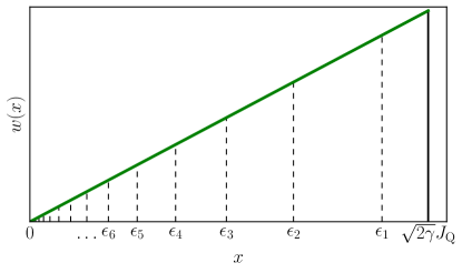
Figure 1: Sketch of the spectral density (34) resulting from the exponential parametrization (3) in the limit of small $\gamma$. In addition, the chosen exponential eigen energies are shown as they result from the procedure explained around Eq. (38) for $\lambda=0.8$.

The SD approach aims at a most efficient representation of the continuous spectral density $w(x)$ by a small number of dynamic variables. Hence, we choose the well-established exponential discretization of the energies in order to capture the long-time behavior. We first define the grid

$$\tilde{\epsilon}_{i}=\lambda^{i}\left(\frac{\epsilon_{\mathrm{max}}(N_{\mathrm{tr}}-i)}{N_{\mathrm{tr}}}\right),\quad i\in\left\{0\dots N_{\mathrm{tr}}\right\},$$ (37)

where $N_{\mathrm{tr}}+1$ is the maximum number of grid points $\tilde{\epsilon}_{i}$ yielding $N_{\mathrm{tr}}$ intervals and $\epsilon_{\mathrm{max}}$ is the maximum value where $w(x)$ is finite, i.e., $\epsilon_{\mathrm{max}}=\sqrt{2\gamma}J_{\text{Q}}$, see Fig. 1. The factor $\lambda<1$ ensures an exponential zoom towards lower frequencies. This factor is chosen according to

$$\lambda=\left(\frac{N_{\mathrm{tr}}}{\epsilon_{\mathrm{max}}t_{\mathrm{max}}}\right)^{\frac{1}{N_{\mathrm{tr}}-1}}.$$ (38)

The guiding idea of the above expression is to identify a maximum time $t_{\mathrm{max}}$ up to which we wish to compute the time evolution. Then, we have to keep the modes with sufficiently low energies such that they precess at most a fraction of a complete turn, i.e., we set $\tilde{\epsilon}_{N_{\mathrm{tr}}-1}t_{\mathrm{max}}=1$. This condition fixes $\lambda$ as given by (38). In rare cases where (38) would yield a value $\lambda>1$ we set $\lambda=1$ refraining from an exponential zoom because the linear discretization is already sufficient.

Finally, the discretization energies $\epsilon_{i}$ are chosen such that they are the average over $w(x)$ between $\tilde{\epsilon}_{i}$ and $\tilde{\epsilon}_{i-1}$

$$\epsilon_{i} :=\left.\int^{\tilde{\epsilon}_{i-1}}_{\tilde{\epsilon}_{i}}x\,w(x)\,\mathrm{d}x\right/\int^{\tilde{\epsilon}_{i-1}}_{\tilde{\epsilon}_{i}}w(x)\,\mathrm{d}x.$$ (39)

This choice guarantees that the weight and the first moment in each of the intervals and hence for the total weight function are correctly represented by the discretization. The finite set of equations is now given by

$$\frac{\mathrm{d}}{\mathrm{d}t}\vec{Q}_{i}(t)=\epsilon_{i}\vec{S}_{0}\times\vec{Q}_{i}(t),\quad i\in\left\{1\dots N_{\mathrm{tr}}\right\}.$$ (40)

Equation (10) still holds and thanks to Eqs. (25) and (29) we know that the Overhauser field $\vec{B}=\vec{P}_{1}$ can be expressed by

$$\vec{P}_{1}=\sum\limits_{i=1}^{N_{\mathrm{tr}}}\sqrt{W_{i}}\vec{Q}_{i}(t),$$ (41)

where $W_{i}$ denotes the weight in the interval $i$

$$W_{i}=\int_{\tilde{\epsilon}_{i-1}}^{\tilde{\epsilon}_{i}}w(x)\,\mathrm{d}x.$$ (42)

Thus, the only free parameter left is the number of intervals $N_{\mathrm{tr}}$, which must be chosen large enough to reach reliable results.

We point out that the exponential discretization advocated above can also be used to efficiently approximate the discrete weight function defined in (31) for finite baths. However, we emphasize that the continuum limit yields excellent results in view of the large number of bath spins in quantum dots. Moreover, it has the conceptually advantageous features (i) to reduce the number of parameters ($N$ drops out) and (ii) to allow for scaling arguments, see below.

IV Results

In the previous section, we have proposed three different algorithms, which aim at enhancing the performance in the computation of dynamical correlations in the classical central spin model. This is crucial to reach long times for large spin baths. While in the full classical simulation the number of differential equations scales proportional to $N$, the proposed algorithms scale proportional to $N_{\mathrm{tr}}\ll N$. Here, we analyze how $N_{\mathrm{tr}}$ has to be chosen to obtain reliable results. Note that the total number of differential equations is given by $3(N_{\mathrm{tr}}+1)$ in all three algorithms. Additionally, we study the dependence of the long-time behavior on the parameter $\gamma$, which is proportional to the inverse effective number of bath spins. We retrieve the long-time scale of the slow dynamics Khaetskii et al. (2003); Coish and Loss (2004), which is essentially given by the inverse of the maximum individual coupling $1/J_{1}$ corresponding to $1/(\sqrt{\gamma}J_{\text{Q}})$. It is a particular strength of the advocated real-time approach that the dynamics on this time scale is accessible.

IV.1 Comparison of all approaches

All numerical data shown has been averaged over $10^{6}$ initial configurations (if not stated otherwise), which are picked at random from Gaussian distributions for all spin components. This approximates the quantum dynamics Stanek et al. (2014).

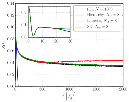
Figure 2: Comparison of the hierarchy, the Lanczos, and the spectral density (SD) approach for fixed truncation parameter $N_{\mathrm{tr}}=8$ with the solution of the full classical simulation for a bath of $N=1000$ spins (except the continuous SD calculation) and $\gamma=0.01$. The inset shows a zoom for short times.

In Fig. 2, we compare the hierarchy, Lanczos and spectral density (SD) approach for the fixed truncation parameter $N_{\mathrm{tr}}=8$ with the numerically exact solution of the full classical simulation for $N=1000$ spins. All algorithms capture the short-time dynamics up to $t\approx 15J_{\mathrm{Q}}^{-1}$ very well. However, the hierarchy approach shows a strong deviation already at $t\approx 20J_{\mathrm{Q}}^{-1}$. Upon increasing $N_{\mathrm{tr}}$ the hierarchy results improve, but very slowly. Hence we conclude that this algorithm is not efficient. We had anticipated this conclusion already in Sect. III.1 and discussed the reasons for it. The general mathematical structure of the hierarchy approach is not appropriate to capture the long-time behavior.

In contrast, both the Lanczos and the SD approach capture the exact solution up to remarkably long times in spite of the fairly small truncation parameter. The Lanczos method starts to deviate at about $t\approx 700J_{\mathrm{Q}}^{-1}$ while the SD approach is close to the exact solution for all displayed times. A deeper understanding of how the results of the Lanczos and the SD approach depend on the truncation parameter $N_{\mathrm{tr}}$ is given in the following two subsections.

IV.2 Lanczos approach

Figure 3: Comparison of the Lanczos approach for various truncation parameters $N_{\mathrm{tr}}$ with the solution of the full classical simulation for $N=1000$ bath spins and $\gamma=0.01$.

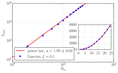
Figure 4: Scaling of the time $t_{\mathrm{max}}$ up to which the Lanczos approach is reliable with the truncation parameter $N_{\mathrm{tr}}$. A power-law fit $t_{\mathrm{max}}\propto N_{\mathrm{tr}}^{a}$ indicates the exponent $a=1.99\pm 0.02$.

Figure 3 shows the dependence of the results of the Lanczos approach on an increasing truncation parameter $N_{\mathrm{tr}}$. It is obvious that after a specific time, the solution starts to deviate from the exact result and displays a spurious plateau region. Up to the specific time the solution is very accurate. In order to know beforehand until which time one may trust the results we introduce the time $t_{\mathrm{max}}$ at which the relative deviation exceeds a certain threshold $\xi$, for instance $\xi=0.1$. In Fig. 4, we study the dependence of $t_{\mathrm{max}}$ on $N_{\mathrm{tr}}$. A power-law fit $t_{\mathrm{max}}\propto N_{\mathrm{tr}}^{a}$ in the double-log plot clearly shows that the scaling is quadratic: $t_{\mathrm{max}}\propto N_{\mathrm{tr}}^{2}$.

Therefore, by increasing the truncation parameter $N_{\mathrm{tr}}$, much longer simulation times can be reached using the Lanczos approach while still having a significant advantage in performance over the full classical simulation.We stress that increasing $N_{\mathrm{tr}}$ does not lead to a deterioration of the description of the short-time dynamics, see inset of Fig. 3.

IV.3 Spectral density approach

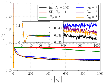
Figure 5: Comparison of results from the spectral density approach to the full classical simulation for various truncation parameters $N_{\mathrm{tr}}$ at $\gamma=0.01$. The full simulation is performed for $N=1000$ bath spins. The wiggles in the right inset result from the averaging over $10^{6}$ initial Gaussian configurations. They scale like the inverse square root of the number of configurations considered in the average.

In contrast to the Lanczos approach, the spectral density (SD) approach shows a completely different behavior upon increasing the truncation parameter $N_{\mathrm{tr}}$ as is illustrated in Fig. 5. As for the Lanczos results the SD results improve upon increasing $N_{\mathrm{tr}}$. But the convergence is roughly uniform, i.e., for low values of $N_{\mathrm{tr}}$ deviations occur for small and for large times and they are of about the same magnitude. We consider this to be an important advantage because we are interested in a faithful description for very long times. It is not a particular asset to have ultrahigh precision at short times.

The reason for this behavior lies in the particular construction of the SD algorithm. The energies, which are included in the description of the bath, are designed to capture all the relevant dynamics in the time interval under study, see Eqs. (37) and (38).

In order to assess the accuracy of the SD approach quantitatively we plot in Fig. 6 the average square difference $\Delta^{2}_{S}$ between the SD result and a highly accurate Lanczos calculation in the time interval under study as function of the truncation parameter $N_{\mathrm{tr}}$. Clearly, we see a rapid convergence, which can be fitted by

$$\Delta^{2}_{S}\approx\frac{A}{N_{\text{tr}}^{B}}+C$$ (43)

with $A=0.009\pm 0.003$, $B=3.9\pm 0.1$, and $C=(1.0\pm 0.1)\cdot 10^{-7}$. The constant offset $C$ occurs naturally because there remains a statistical error for all $N_{\text{tr}}$ from the average over $10^{7}$ random Gaussian initial values. The fit clearly shows that the average convergence is quadratic $\Delta_{S}\propto 1/N_{\text{tr}}^{2}$ in the inverse number $N_{\text{tr}}$ of tracked dynamic vectors.

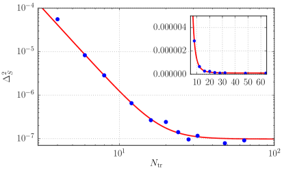
Figure 6: Average square difference $\Delta^{2}_{S}$ between the SD result and an accurate Lanczos result in the continuum limit. The average is computed in the time interval $t\in[50,10000]J_{\text{Q}}^{-1}$. The solid line depicts the fit (43) which is obtained for values from $N_{\text{tr}}=8$ onwards.

The advantageous feature of the SD approach is summarized in Fig. 7, which clearly shows that that the SD approach captures the dynamics of the central spin model more efficiently than the Lanczos approach. We stress, however, that the Lanczos approach has the advantage to yield particularly precise data when simulating shorter times. Both approaches can deal with nominally infinitely large spin baths, i.e., for $N=\infty$, while the effective number of bath spins $N_{\mathrm{eff}}$ is finite corresponding to a finite parameter $\gamma=2/N_{\mathrm{eff}}$.

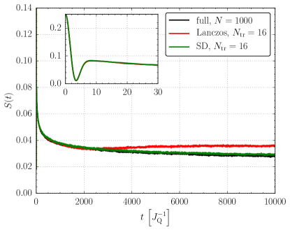
Figure 7: Comparison of results from the Lanczos and the spectral density approach for $N_{\mathrm{tr}}=16$ to the full classical simulation for very long times up to $t=10000J_{\mathrm{Q}}^{-1}$ at $\gamma=0.01$. The Lanczos and the full calculations are performed for $N=1000$ bath spins.

IV.4 Long-time behavior

Above, we have illustrated that the spectral density approach is especially suited to describe the dynamics at very long times correctly. Hence, we adopt this algorithm for the subsequent analysis. We use $N_{\mathrm{tr}}=32$ for the following calculations. Note that the calculations are carried out for infinitely large baths $N=\infty$.

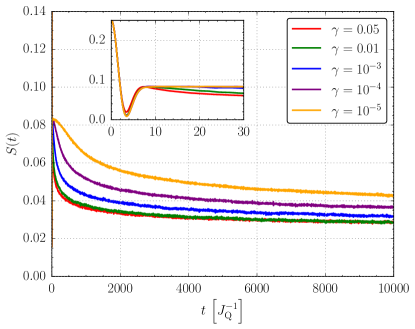
Figure 8: Dynamics for various values of $\gamma$ for very long times up to $t=10^{4}J^{-1}_{\text{Q}}$ from the SD approach. The calculations are performed for $N=\infty$ bath spins and $N_{\mathrm{tr}}=32$.

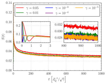
Figure 9: Rescaled results from Fig. 8 showing an excellent data collapse as long as the short-time dynamics and the long-time dynamics are separated clearly, i.e., for $\sqrt{\gamma}\ll 1$.

We investigate the influence of the parameter $\gamma$, which represents the inverse number of effectively coupled bath spins. Figure 8 shows a set of representative results for various values of $\gamma$ up to $t=10^{4}J_{\mathrm{Q}}^{-1}$. While the curves are qualitatively very similar, smaller values of $\gamma$ clearly imply a slower long-time dynamics. We stress that the short-time dynamics, see inset, is not altered by changing $\gamma$ because it is determined by the energy scale $J_{\mathrm{Q}}$, which is the energy scale used throughout this article, i.e., it is set to unity in the numerics. Hence, all curves coincide in the inset. Only the $\gamma=0.05$ curve deviates a tiny bit. We attribute this effect to the fact that at $\gamma=0.05$ the continuum limit, i.e., the step from (33a) to (33b), does not capture the discrete bath perfectly.

Turning back to the long-time dynamics the question arises whether the dynamics for different values of $\gamma$ can be mapped on one curve. This would imply that the information content is essentially the same. Practically, a good data collapse would help future theoretical simulations since only moderate values of $\gamma$ need to be analyzed.

Looking at Fig. 1 and at the analytic result (34) it is obvious that the maximum energy occurring in the weight function $w(x)$ sets a second energy scale. This energy scale is $\sqrt{\gamma}J_{\mathrm{Q}}$. The first energy scale is $J_{\mathrm{Q}}$ as discussed above for the inset of Fig. 8. Hence, it is natural to assume that the long-time dynamics is determined by the second, much smaller energy scale $\sqrt{\gamma}J_{\mathrm{Q}}$. To corroborate this hypothesis we plot the data from Fig. 8 with rescaled time argument in Fig. 9. Indeed, an impressive data collapse is achieved. In particular for low values of $\gamma$, the scaling with $\sqrt{\gamma}$ works perfectly. For larger values of $\gamma$, the two energy scales $J_{\mathrm{Q}}$ and $\sqrt{\gamma}J_{\mathrm{Q}}$ are not so clearly separated so that the rescaling is not fully quantitative.

Obviously, the short-time dynamics does not match anymore once the rescaling with the factor $\sqrt{\gamma}$ has been performed, see inset of Fig. 9. This is so because the corresponding time scale is solely given by $J_{\mathrm{Q}}^{-1}$.

Another issue is how the correlations in the central spin model decrease. In the quantum mechanical model we know from rigorous lower bounds Uhrig et al. (2014); Seifert et al. (2016) that the correlations never fade away, but persist even for infinite baths if the couplings are distributed such that their distribution can be described as probability distribution $p(J)$ with finite moments. Note that this is not the case for the exponentially parametrized couplings in (3) and the Gaussian parametrizations considered in Appendix B because these parametrizations imply that there are an infinite number of very weakly coupled spins. No normalization of a probability distribution $p(J)$ is possible.

We recall that the lower bounds as discussed in Refs. Uhrig et al. (2014); Seifert et al. (2016) result from the existence of conserved quantities such as the total angular momentum and the total energy. These quantities are conserved also for the classical model and the choices of couplings we are considering here. Hence it is not astounding that the correlations live very long. They are protected by conservation laws and thus they decrease very slowly as can be seen in Figs. 7, 8, and 9.

The question arises how the slow decay can be described quantitatively. Chen et al. proposed a slow logarithmic decay Chen et al. (2007). Hence we fit the simulated data according to

$$S(t)=A/\ln^{B}(t/t_{0}).$$ (44)

The simulated data and the fit are compared in Fig. 10. The fit has been obtained in the interval $t\in[10^{3},10^{4}]J^{-1}_{\text{Q}}$. Clearly, it works very well, supporting Chen’s suggestion. The fit parameters are $A=0.243\pm 0.001$, $B=0.954\pm 0.002$, and $t_{0}=(0.81\pm 0.01)/J_{\mathrm{Q}}$. The fit is of comparable quality if we fixed $B=1$. So the existence of a logarithmic factor is certain, but further details such as the precise power, let alone further logarithmic corrections Seifert et al. (2016), cannot be determined reliably.

There is no need to show and to analyze data for other values of $\gamma$ due to the above established scaling with $\sqrt{\gamma}$ for sufficiently small values of $\gamma$.

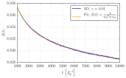
Figure 10: Analysis of the long-time behavior of the correlations, computed from $10^{8}$ initial Gaussian configurations for enhanced accuracy, by a logarithmic fit (44). The parameters are given in the main text.

Finally, we address the influence of varying weight functions. We do not study wildly different weight functions, but stay with plausible choices. The dominant hyperfine coupling is proportional to the probability of the electron to be present at the position of the nuclear spins in the quantum dot Merkulov et al. (2002); Schliemann et al. (2003). Assuming to first approximation a parabolic trapping potential as it results from any Taylor expansion, Gaussian wave functions are the most plausible assumption. In Appendix B, we compute the three corresponding weight functions $w_{d}(x)$ in dimension $d=1,2$, and $3$. The two-dimensional (2D) case is covered by the linear weight function, which we have used so far.

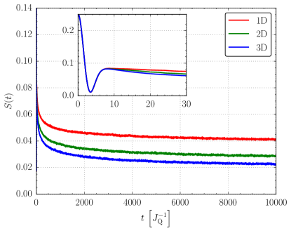
Figure 11: Comparison of the dynamics of the spin-spin correlation in the central spin model for three generic weight functions $w_{d}(x)$ relevant in dimension $d=1$ (1D), $d=2$ (2D), and $d=3$ (3D) for $\gamma=0.01$. The weight functions are given in Eqs. (53b), (59b), and (65b). Note that the 2D Gaussian case is identical to the linear weight function $w(x)$ in (34).

In Fig. 11, we compare the resulting dynamic correlation for the same value of $\gamma=0.01$, which implies the same number of effectively coupled bath spins. The results indicate that the influence of the dimensionality is only moderately important. The main feature of a very slowly, logarithmically decaying correlation is found in all dimensions. The same is true for the scaling $\sqrt{\gamma}\propto 1/\sqrt{N_{\mathrm{eff}}}$.

V Conclusions

We considered the central spin model as relevant description of two-level systems coupled to large spin baths. While the quantum model is the ultimate aim in order to describe the experimental results, it has been shown that classical simulations averaged appropriately over Gaussian distributed initial conditions provide very good approximations Al-Hassanieh et al. (2006); Chen et al. (2007); Stanek et al. (2014). Thus our study aimed at establishing efficient approaches to deal with the averaged classical central spin model. Two demanding challenges had to be met: very large numbers of bath spins and very long times.

Instead of addressing single spins we introduced generalized higher Overhauser fields, which promise to yield a much more efficient approach. A first attempt, the hierarchy approach, failed due to an inappropriate mathematical structure. However, the Lanczos and the spectral density (SD) approach turned out to be extremely powerful because they require to track only 10-100 vectors. The number of these vectors, denoted $N_{\mathrm{tr}}$, is the control parameter of the accuracy of the approaches.

The Lanczos approach displays a non-uniform convergence being excellent up to a certain threshold in time $t_{\mathrm{max}}$, which can be pushed higher and higher by increasing $N_{\mathrm{tr}}$. The scaling is $t_{\mathrm{max}}\propto N_{\mathrm{tr}}^{2}$. The Lanczos approach is particularly well suited if high-precision data is required for not too long times.

The SD approach is adjusted to a pre-set time interval. Within this interval it displays a uniform quadratic convergence at very moderate computational cost. Moreover, it is based on the appealing concept of a continuum limit, which amounts to setting the total number of bath spins to infinity while the number $N_{\mathrm{eff}}$ of sizeably coupled bath spins within the localization volume of the electronic central spin is kept as relevant parameter. In order to establish an appropriate continuum limit, we introduced weight functions and determined them in the generic cases.

Employing the powerful SD approach we identified the energy scale, which is responsible for the long-time behavior. This low-energy scale is given by $\propto J_{\mathrm{Q}}/\sqrt{N_{\mathrm{eff}}}$ where $J_{\mathrm{Q}}$ is the root of the square sum of all couplings. The energy $J_{\mathrm{Q}}$ is known to dominate the short-time behavior Merkulov et al. (2002); Stanek et al. (2013). The low-energy scale $J_{\mathrm{Q}}/\sqrt{N_{\mathrm{eff}}}$ has appeared in previous investigations Khaetskii et al. (2003); Coish and Loss (2004). However, we emphasize that the above introduced algorithm can produce reliable real-time data up to these very long time scales for infinite baths with very large effective number of nuclear spins. This allowed us to show by explicit and systematically controlled calculation that the rescaling of the long-time tails of the spin-spin correlation with the low-energy scale achieves a convincing data collapse, see Fig. 9.

Physically, the low-energy scale $J_{\mathrm{Q}}/\sqrt{N_{\mathrm{eff}}}$ is obviously a representative value of the individual couplings of the bath spins. This observation appears to be highly plausible because the individual bath spin $i$ can react to the behavior of the central spin only by the rate $J_{i}/\hbar$. As long as the bath itself remains static the spin-spin correlation of the central spin does not decay but remains constant at one third of its initial value Merkulov et al. (2002); Stanek et al. (2013). Hence, further decay will be slow and can happen only at the rate at which the bath spin precess.

Finally, we studied the influence of the dimensionality of the electronic wave function by computing the different weight functions $w_{d}(x)$. The resulting dynamics, however, indicates only a moderate dependence on the dimensionality. This observation also implies that the details of the couplings in a quantum dot do not matter much. The key parameters are the high-energy and the low-energy scale dominating the short-time and the long-time behavior, respectively.

The established approaches and the above observations provide a reliable algorithmic and conceptual foundation for many further investigations. The approach is straightforwardly extended to finite external magnetic fields acting on the central spin or on the bath spins. In particular, studies of pulsed quantum dots in external magnetic fields are called for Greilich et al. (2006, 2007); Petrov and Yakovlev (2012); Economou and Barnes (2014); Beugeling et al. (2016, 2017).

Appendix A Lanczos approach

The starting point is $p_{1}(x)=x$, which is a bit unusual compared to standard orthogonal polynomials which start at $p_{1}=1$. For the iteration we assume that the recursion

$$xp_{m}(x)=\beta_{m}p_{m+1}(x)+\alpha_{m}p_{m}(x)+\beta_{m-1}p_{m-1}(x)$$ (45)

for orthonormalized $p_{m}$ holds up to $m=n-1$. The next step of the induction iterates $\tilde{p}_{n+1}:=xp_{n}$ where the tilde indicates that this polynomial is not yet the next orthonormalized polynomial. The overlaps with already defined polynomials read

$$\left(\tilde{p}_{n+1}|\tilde{p}_{n-1}\right)=\left(p_{n}xp_{n-1}\right)=\beta_{n-1}.$$ (46)

We compute and define

$$\alpha_{n} :=\left(\tilde{p}_{n+1}|{p}_{n}\right)$$ (47a)

$$\beta_{n} :=\sqrt{\left|\tilde{p}_{n+1}-\alpha_{n}p_{n}-\beta_{n-1}p_{n-1}\right|^{2}}$$ (47b)

$$p_{n+1}(x) :=\frac{1}{\beta_{n}}\left(\tilde{p}_{n+1}-\alpha_{n}p_{n}-\beta_{n-1}p_{n-1}\right).$$ (47c)

A straightforward calculation confirms that $p_{n+1}$ defined in this way obeys (45) for $m=n$ and is orthonormalized with respect to all previously defined polynomials.

We stress that the above construction does not require that the spin bath is finite. As long as the scalar product in (17) is well defined, i.e., converges, the Lanczos approach works.

Appendix B Weight Functions

In the main text we established the linear weight function (34) implied by the exponentially parametrized couplings (3). Here we supplement this finding by three other generic Gaussian parametrizations of the couplings.

B.1 One-dimensional Gaussian parametrization

We consider

$$J_{i}=C\exp(-\alpha^{2}i^{2})$$ (48)

with $i\in\{1,2,3,\ldots\}$. For small values of $\alpha$ it is justified to approximate the sums over all couplings by integrals. For the energy scale $J_{\mathrm{Q}}^{2}$ we obtain

$$J_{\mathrm{Q}}^{2} =\sum_{i}J_{i}^{2}$$ (49a)

$$=\frac{C^{2}}{\alpha}\int_{0}^{\infty}\exp(-2y^{2})\mathrm{d}y$$ (49b)

$$=\frac{C^{2}\sqrt{2\pi}}{4\alpha}.$$ (49c)

Analogously, one obtains

$$J_{\mathrm{S}} =\sum_{i}J_{i}$$ (50a)

$$=\frac{C}{\alpha}\int_{0}^{\infty}\exp(-y^{2})\mathrm{d}y$$ (50b)

$$=\frac{C\sqrt{\pi}}{2\alpha}$$ (50c)

so that the number of effective bath spins $N_{\mathrm{eff}}=J_{\mathrm{S}}^{2}/J_{\mathrm{Q}}^{2}$ is given by

$$N_{\mathrm{eff}} =\sqrt{\frac{\pi}{2}}\frac{1}{\alpha}.$$ (51)

Hence, setting $\alpha=\sqrt{\frac{\pi}{8}}\gamma$ implies $\gamma=2/N_{\mathrm{eff}}$ as before. We opt for this choice of $\alpha$ for better comparability. The energy constant $C$ results to be

$$C =\sqrt{\gamma}J_{\mathrm{Q}}$$ (52)

and the weight function to be

$$w_{1}(x) =\frac{x^{2}}{\alpha}\int_{0}^{\infty}\delta(x-C\exp(-y^{2}))\mathrm{d}y$$ (53a)

$$=\frac{x\theta(x(C-x))}{\gamma\sqrt{\pi\ln(C/x)/2}}.$$ (53b)

It is compared in Fig. 12 to other weight functions with the same value of $\gamma$, i.e., the same number of effectively coupled spins.

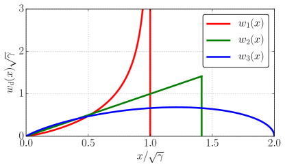
Figure 12: Comparison of three weight functions $w_{d}(x)$ resulting from Gaussian parametrized couplings in $d$ dimensions. The linear weight function of the two-dimensional Gaussian equals the one of a one-dimensional exponential as discussed in the main text. This fact underlines the relevance of the linear weight function.

B.2 Two-dimensional Gaussian parametrization

We consider

$$J_{r}=C\exp(-\alpha^{2}r^{2})$$ (54)

where $r$ is a two-dimensional vector $r\in\mathds{Z}^{2}$. For small values of $\alpha$ it is justified to approximate the sums over all couplings by integrals. For the energy scale $J_{\mathrm{Q}}^{2}$ we obtain

$$J_{\mathrm{Q}}^{2} =\sum_{r}J_{r}^{2}$$ (55a)

$$=\frac{2\pi C^{2}}{\alpha}\int_{0}^{\infty}y\exp(-2y^{2})\mathrm{d}y$$ (55b)

$$=\frac{\pi C^{2}}{2\alpha}.$$ (55c)

Analogously, one obtains

$$J_{\mathrm{S}} =\sum_{r}J_{r}$$ (56a)

$$=\frac{2\pi C}{\alpha}\int_{0}^{\infty}y\exp(-y^{2})\mathrm{d}y$$ (56b)

$$=\frac{\pi C}{\alpha}$$ (56c)

so that the number of effective bath spins $N_{\mathrm{eff}}=J_{\mathrm{S}}^{2}/J_{\mathrm{Q}}^{2}$ is given by

$$N_{\mathrm{eff}} =\frac{2\pi}{\alpha}.$$ (57)

Hence, setting $\alpha=\pi\gamma$ implies $\gamma=2/N_{\mathrm{eff}}$ as before for better comparability. The energy constant $C$ results to be

$$C =\sqrt{2\gamma}J_{\mathrm{Q}}$$ (58)

and the weight function reads

$$w_{2}(x) =\frac{2\pi x^{2}}{\alpha}\int_{0}^{\infty}y\delta(x-C\exp(-y^{2}))\mathrm{d}y$$ (59a)

$$=\frac{x\theta(x(C-x))}{\gamma}.$$ (59b)

We note that the Gaussian couplings in two dimensions yield precisely the same weight function as the exponential couplings (3) in one dimension, see also Fig. 12.

B.3 Three-dimensional Gaussian parametrization

We consider

$$J_{r}=C\exp(-\alpha^{2}r^{2})$$ (60)

where $r$ is a three-dimensional vector $r\in\mathds{Z}^{3}$. For small values of $\alpha$ it is justified to approximate the sums over all couplings by integrals. For the energy scale $J_{\mathrm{Q}}^{2}$ we obtain

$$J_{\mathrm{Q}}^{2} =\sum_{r}J_{r}^{2}$$ (61a)

$$=\frac{4\pi C^{2}}{\alpha}\int_{0}^{\infty}y^{2}\exp(-2y^{2})\mathrm{d}y$$ (61b)

$$=\frac{C^{2}}{\alpha}\left(\frac{\pi}{2}\right)^{3/2}.$$ (61c)

Analogously, one obtains

$$J_{\mathrm{S}} =\sum_{r}J_{r}$$ (62a)

$$=\frac{4\pi C}{\alpha}\int_{0}^{\infty}y^{2}\exp(-y^{2})\mathrm{d}y$$ (62b)

$$=\frac{\pi^{3/2}C}{\alpha}$$ (62c)

so that the number of effective bath spins $N_{\mathrm{eff}}=J_{\mathrm{S}}^{2}/J_{\mathrm{Q}}^{2}$ is given by

$$N_{\mathrm{eff}} =\frac{(2\pi)^{3/2}}{\alpha}.$$ (63)

Hence, setting $\alpha=(2\pi)^{3/2}\gamma/2$ implies $\gamma=2/N_{\mathrm{eff}}$ as before for better comparability. The energy constant $C$ results to be

$$C =2\sqrt{\gamma}J_{\mathrm{Q}}$$ (64)

and the weight function reads

$$w_{3}(x) =\frac{4\pi x^{2}}{\alpha}\int_{0}^{\infty}y^{2}\delta(x-C\exp(-y^{2}))\mathrm{d}y$$ (65a)

$$=\sqrt{\frac{2}{\pi}}\frac{x}{\gamma}\theta(x(C-x))\sqrt{\ln(C/x)}.$$ (65b)

This weight function is compared to the other generic ones in Fig. 12. We note that the differences are not very large since they result from square roots of logarithmic factors only.