Topological recursion and geometry

Website: guests.mpim-bonn.mpg.de/gborot/Teach.html 052017 Mini-course, Institut Mathématique de Toulouse, France.

These are lecture notes for a 4h mini-course held in Toulouse, May 9-12th, at the thematic school on

Quantum topology and geometry

I thank Francesco Costantino and Thomas Fiedler for organization of this event, the audience and especially Rinat Kashaev and Gregor Masbaum for questions and remarks which improved the lectures.

Imagine you have a problem to solve concerning surfaces of genus $g$ with $n$ boundaries/marked points. A topological recursion is a strategy consisting of

• solving the problem for the simplest topologies, i.e. disks $(g,n)=(0,1)$, cylinders $(g,n)=(0,2)$, pairs of pants $(g,n)=(0,3)$.

• understanding how the problem behaves when one glues together pairs of pants – or conversely, when one removes a pair of pants/degenerates the surface. You can then solve the problem by induction on $\chi_{g,n}=2g-2+n=-$(the Euler characteristic of the surface).

This mantra is realized in several different ways in geometry and quantum field theories. The topological recursion (tr) in these lectures refers to an abstract formalism tailored to handle this kind of recursion at the numerical level. When tr applies, it often shadows finer geometric properties which depend on the problem at studied.

The goal of these lectures is to (a) explain some incarnations, in the last ten years, of the idea of topological recursion: in two dimensional quantum field theories (2d tqfts), in cohomological field theories (cohft), in the computation of volumes of the moduli space of curves; (b) relate them to tr.

Sources. The perspective we adopt here on tr was proposed lately by Kontsevich and Soibelman [KSTR] based on the notion of quantum Airy structure. This was further studied by Andersen, the author, Chekhov and Orantin [TRABCD], and we often borrow arguments from this paper. The original formulation of tr was proposed by Eynard and Orantin [EOFg] using spectral curves, but quantum Airy structures allows a simpler, more algebraic, and slightly more general presentation of the possible initial data for tr. Part of Chapter 2 on 2d tqfts is inspired from [Abrams]. The exposition of Givental group action in Chapter 4 is inspired from [Zvonkin]. Chapter 5 is inspired from Mirzakhani [Mirza1] and Wolpert exposition of her works [Wolpertlecture].

[1h]09052017

1 Quantum Airy structures

1.1 First principles

The initial data for tr is a “quantum Airy structure”. This notion was introduced by Kontsevich and Soibelman in [KSTR]. Let $V$ be a vector space over a field $\mathbb{K}$ of characteristic $0$. Let $(e_{i})_{i\in I}$ be a basis of $V$, and $(x_{i})_{i\in I}$ the corresponding basis of linear coordinates. $\hbar$ denotes a formal parameter. If $V$ is infinite dimensional, we may have to add assumptions (filtration, completion, convergence) so that all expressions we write make sense. We will overlook this issue, and in the examples of quantum Airy structures with $\dim V=\infty$ we meet, it is possible to check that seemingly infinite sums we are going to write actually contain only finitely many non-zero terms.

Definition 1.1.

A quantum Airy structure on $V$ is the data of a family of differential operators $(L_{i})_{i\in I}$, of the form L_i = ℏ∂_x_i - ∑_a,b ∈I ( 12 A^i_a,bx_ax_b + ℏ B^i_a,bx_a∂_x_b + ℏ22 C^i_a,b∂_x_a∂_x_b) - ℏD^i , and such that ∀i,j ∈I,  [L_i,L_j] = ∑_a ∈I ℏ f_i,j^a L_a , where $A^{i}_{j,k}=A^{i}_{k,j}$, $B^{i}_{j,k}$, $C^{i}_{j,k}=C^{i}_{k,j}$, $D^{i}$, $f^{i}_{j,k}=-f^{i}_{k,j}$ are scalars indexed by $i,j,k\in I$.

$\bullet$ The six conditions. The condition (1.1) says that $(L_{i})_{i\in I}$ span a Lie algebra with structure constants $(f_{i,j}^{k})_{i,j,k\in I}$. This is equivalent to a system of six constraints on $(A,B,C,D,f)$.

The identification of the $\partial_{x_{k}}$ terms, and of the $x_{k}$ terms, in both sides of (1.1) yields the two linear relations ∀i,j,k ∈I,  f_i,j^k = B^i_j,k - B^j_i,k,  A^i_j,k = A^j_i,k . We use these two relations to get rid of $f$ in the four remaining relations. Identification of the constant term yields ∀i,j,k,ℓ∈I,  ∑_a ∈I B^i_j,aD^a + ∑_a,b ∈I C^i_a,bA^j_a,b = (i ↔j) . If $(A,B,C)$ are known, this relation is affine in $D$. Then, identification of $x_{k}x_{\ell}$, $x_{k}\partial_{x_{\ell}}$ and $\partial_{x_{k}}\partial_{x_{\ell}}$ yields ∀i,j,k,ℓ∈I,  {∑_a ∈I B^i_j,aA^a_k,ℓ + B^i_k,aA^j_a,ℓ + B^i_ℓ,aA^j_a,k=(i ↔j)∑_a ∈I B^i_j,aB^a_k,ℓ + B^i_k,aB^j_a,ℓ + C^i_ℓ,aA^j_a,k=(i ↔j)∑_a ∈I B^i_j,aC^a_k,ℓ + C^i_k,aB^i_a,ℓ + C^i_ℓ,aB^i_a,ℓ=(i ↔j) . These three quadratic relations have the same index structure. In fact, they form a system of three coupled IHX-type relations (Figure 1). The relation involving $D$ is depicted in Figure 2.

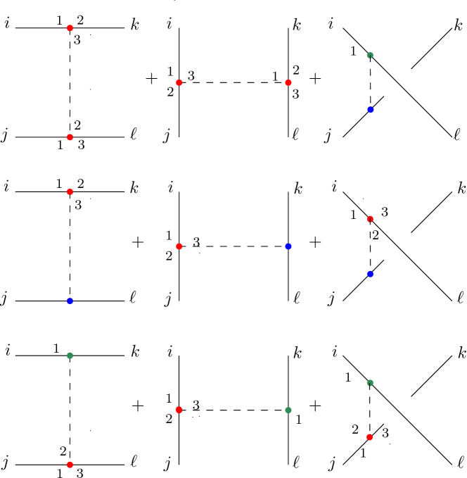
Figure 1: A red dot is replaced by a $B$, a green dot by a $C$, a blue dot by an $A$. The labels $1,2,3$ specify the ordering of indices at a $B$-vertex, namely $B^{i_{1}}_{i_{2},i_{3}}$, and $1$ at $C$-vertex specifies the first index $C^{i_{1}}_{**}$. Such an ordering is not necessary at an $A$-vertex as $A$ is fully symmetric. The dashed line carries an index $a\in I$ which is summed over. Equation (1.1) says that each of the three lines is symmetric under permutation of $i$ and $j$.

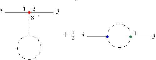
Figure 2: The loop carries an index $a\in I$ which is summed over, and stands for $D^{a}$. Equation (1.1) says that this expression is symmetric under permutation of $i$ and $j$.

$\bullet$ Counting. If $\dim V=d$, let us count the number of unknowns and independent conditions determining a quantum Airy structure. As (1.1) fixes $f$ in terms of $B$, and $A$ is fully symmetric, there remains

$$\#{\rm unknowns}=\underbrace{\tfrac{d(d+1)(d+2)}{6}}_{A}+\underbrace{d^{3}}_{B}+\underbrace{\tfrac{d^{2}(d+1)}{2}}_{C}+\underbrace{d}_{D}=\tfrac{d(5d^{2}+3d+4)}{3}\,.$$

The independent relations are indexed by the unordered pair $\{i,j\}\subseteq I$, and for (1.1) by $k,\ell\in I$. In fact, $k$ and $\ell$ play a symmetric role in the BA and BC relations. So

$$\#{\rm relations}=\tfrac{d(d-1)}{2}\big{(}1+\tfrac{d(d+1)}{2}+d^{2}+\tfrac{d(d+1)}{2}\big{)}=\tfrac{d(d-1)(2d^{2}+d+1)}{2}\,.$$

The number of relations grows faster – like $d^{4}$ – than the number of unknowns – which grows like $d^{3}$. For small values of $d$, we have

$$\begin{array}[]{|c|c|c|c|c|c|c|}\hline\cr d&1&2&3&4&5&6\\ \hline\cr\hline\cr\#\,{\rm unknowns}&4&20&58&128&240&404\\ \hline\cr\#\,{\rm relations}&0&11&66&222&560&1185\\ \hline\cr\end{array}$$

Therefore, for $d\geq 3$ the system of relations is overdetermined, and it is not clear that quantum Airy structures can exist at all. In fact, the size of this system of quadratic relations makes difficult, even for small $d$, to obtain solutions by brute computer force. We will see that quantum Airy structure do exist, and in all examples we know of, they are tied to geometry.

$\bullet$ Basis-free definition. Although we presented the definition of quantum Airy structures using a basis, we now explain how it can be made a basis-independent notion. Let $\mathcal{W}_{V}$ be the Weyl algebra of $V$, that is the quotient of the free algebra generated by $\mathbb{K}[\hbar]\oplus V\oplus V^{*}$, by the relations

$$\forall v_{1},v_{2}\in V,\quad\forall\ell_{1},\ell_{2}\in V^{*},\qquad[\ell_{1},\ell_{2}]=[v_{1},v_{2}]=0,\qquad[v_{1},\ell_{1}]=\hbar\ell_{1}(v_{1})\,.$$

The elements of $V\subset\mathcal{W}$ are the derivations $\hbar\partial_{x_{i}}$, and the elements of $V^{*}\subseteq\mathcal{W}_{V}$ are the linear coordinates $x_{i}$ on $V$. We equip $\mathcal{W}_{V}$ with two notions of degree, compatible with the algebra structure. The first one counts $x_{i}$ and $\hbar\partial_{x_{i}}$, namely ${\rm deg}\,V={\rm deg}\,V^{*}=1$ and ${\rm deg}\,\mathbb{K}[\hbar]=0$. We denote $\mathcal{W}_{V}(d)$ – resp. $\mathcal{W}_{V}(\leq d)$ – the subspace spanned by elements of degree $d$ – respectively, less or equal to $d$. The second one is the usual $\hbar$-degree on $\mathbb{K}[\hbar]$, supplemented by the assignments ${\rm deg}_{\hbar}V={\rm deg}_{\hbar}\,V^{*}=0$. In other words, $\hbar^{k}x^{\ell}\partial^{m}$ has $\hbar$-degree $(k-m)$. This convention may seem unnatural, but it is convenient for the next definition.

We remark that $\mathcal{W}_{V}(\leq 2)$ is a Lie algebra, while $\mathcal{W}_{V}(\leq d)$ is not $d\geq 3$ as can be seen from degree counting. This justifies considering operators of degree at most $2$. We denote $\pi_{d}$ and $\pi_{\leq d}$ the projection onto the subspaces $\mathcal{W}_{V}(d)$ and $\mathcal{W}_{V}(\leq d$).

Definition 1.2.

A quantum Airy structure on $V$ is the data of a Lie algebra structure on $V$ and a homomorphism of Lie algebras $L\,:\,V\rightarrow\mathcal{W}_{V}(\leq 2)$ such that

• ${\rm Im}(\pi_{1}\circ L)=V\subseteq\mathcal{W}_{V}(1)$, and $\pi_{1}\circ L$ induces an isomorphism $\varphi\,:\,V\rightarrow V\subseteq\mathcal{W}_{V}(1)$.

• for $d\in\{0,1,2\}$, we have ${\rm deg}_{\hbar}(\pi_{d}\circ L)=\delta_{d,0}$.

As $\mathcal{W}_{V}(2)=\big{(}{\rm Sym}^{2}(V^{*}\oplus V)\big{)}[\hbar]$ and taking into account the $\hbar$-degree condition, $\pi_{2}\circ L$ decomposes into three tensors. Turning a $V^{*}$ in the target to a $V$ in the source, they can be arranged as

$$A\in{\rm Hom}_{\mathbb{K}}(V^{\otimes 3},\mathbb{K}),\qquad B\in{\rm Hom}_{\mathbb{K}}(V^{\otimes 2},V),\qquad C\in{\rm Hom}_{\mathbb{K}}(V,V^{\otimes 2})\,.$$

Besides, $\hbar^{-1}(\pi_{0}\circ L)$ gives

$$D\in{\rm Hom}_{\mathbb{K}}(V,\mathbb{K})\,.$$

The conditions (1.1)-(1.1)-(1.1) on $(A,B,C,D)$ expressing that $L$ is a Lie algebra morphism can written solely in terms of composition of these morphisms. In fact, they would make sense in the more general context of $V$ being an object in a symmetric monoidal category – here we worked with the category $\mathbf{Vect}_{\mathbb{K}}$ of finite-dimensional $\mathbb{K}$-vector fields.

The relation between Definitions 1.1 and 1.2 is as follows. If $(e_{i})_{i\in I}$ is a basis of $V$, we should consider it as a basis of $V\subseteq\mathcal{W}_{V}$ and then $L_{i}=L(\varphi^{-1}(e_{i}))$ for all $i\in I$.

1.2 Partition function and topological recursion

Taking a quantum Airy structure $L$ as input, we can get a function on $V$ which is simultaneously annihilated by the differential operators given by $L$. More precisely, the output $F$ will belong to the space E_V = ℏ