User Selection and Widely Linear Multiuser Precoding for One-dimensional Signalling

Abstract

Massive deployment of low data rate Internet of things and ehealth devices prompts us to develop more practical precoding and user selection techniques that comply with these requirements. Moreover, it is known that when the data is real-valued and the observation is complex-valued, widely linear (WL) estimation can be employed in lieu of linear estimation to improve the performance. With these motivations, in this paper, we study the transmit precoding (beamforming) in multiuser multiple-input single-output communications systems assuming the transmit signal is one-dimensionally modulated and widely linear estimation is performed at the receivers. Closed-form solutions for widely linear maximum ratio transmission (MRT), WL zero-forcing (ZF), WL minimum mean square error (MMSE), and WL maximum signal to leakage and noise ratio (MSLNR) precoding are obtained. It is shown that widely linear processing can potentially double the number of simultaneous users compared to the linear processing of one-dimensionally modulated signals. Furthermore, to deal with the increasing number of communications devices a user selection algorithm compatible with widely linear processing of one-dimensionally modulated signals is proposed. The proposed user selection algorithm can double the number of simultaneously selected users compared to conventional user selection methods.

I Introduction

Widely linear (WL) processing of complex-valued signals, originally introduced in [1] and later resurrected in [2] in the context of minimum mean square error estimation, refers to the superposition of linear filtering of the observation and linear filtering of its complex conjugate, or equivalently, superposition of linear filtering of real and imaginary parts [3]. The latter representation is known as the composite real representation. It was shown in [2] that when the distribution of the estimand (signal of interest) is improper, i.e., not circularly symmetric, widely linear estimation will improve mean square error (MSE) estimation, whether or not the observation is improper. Since its resurrection by Picinbono and Chevalier [2], WL processing has been applied to communications systems, specifically to improper signal constellations or when improper noise is encountered [3, 4].

Advances in wireless communications, in conjunction with advances in electronics, paved the way for emergence of technologies including the Internet of things (IoT) and pervasive ubiquitous ehealth [5, 6, 7, 8]. In wireless communications, low-data-rate power efficient one-dimensionally (1D) modulated signals such as binary phase shift keying (BPSK) are of interest to reliably support these emerging systems with massive numbers of low-data-rate devices [9, 6]. When the data is one-dimensionally modulated, implying an improper distribution, widely linear estimation has been applied to receive beamforming in the context of multiple-antenna communications [10, 11, 12, 13]. In contrast to linear receive beamforming, in which the output is given by a linear spatial filter ${\bf w}$ applied to received signal ${\bf r}$ as $y={\bf w}{\bf r}$, a widely linear receive beamformer output is given by $y={\bf w}{\bf r}+{\bf v}{\bf r}^{*}$, which includes superposition of linear beamforming ${\bf v}$ of the complex conjugate of the received signal. For the special case of one-dimensionally modulated signals, widely linear receive beamforming reduces to the real part of the linearly filtered observation, i.e., $y=\Re\{{\bf w}{\bf r}\}$ [2].

The concept of widely linear processing can also be applied to transmit precoding (beamforming). From one perspective, widely linear precoding is the superposition of linear precoding of the modulated signal and linear precoding of the complex conjugate of the modulated signal [14]. From another perspective, widely linear precoding is the linear precoding of the modulated signal in conjunction with widely linear estimation of the received signal [15]. It should be remarked that if the modulated signal is real-valued, only the latter perspective of widely linear transmit precoding is relevant.

In wireless systems, the base station or access point may be equipped with multiple antennas and users are typically equipped with a single antenna due to physical constraints such as equipment size, power supply, cost, and computational capabilities [16]. Consequently, the downlink transmitter can transmit different data streams to multiple users simultaneously to exploit the available spatial multiplexing gain. The task of transmit precoding is to reduce the effect of co-channel interference which arises in wireless broadcast channels due to spatial multiplexing. Four basic linear transmit precoders that are well researched in the last decades are: (i) transmit matched filtering or maximum ratio transmission (MRT) precoding which maximizes the signal portion of the desired signal at each receiver [17], (ii) transmit zero-forcing or channel inversion precoding which nulls the interference at each receiver [18, 17], (iii) transmit minimum mean square error or regularized channel inversion precoding which minimizes sum of mean square errors (MSE) of users [19, 18, 17], and (iv) maximum signal to leakage and noise ratio (MSLNR) precoding [20]. In this paper, we develop widely linear counterparts of these four basic linear precoding techniques for one-dimensional signalling.

As mentioned earlier, emerging applications such as IoT and ehealth traffic require support of a large number of low-data-rate users. To support large numbers of devices, one of the challenging issues is network traffic. One approach to reduce the network traffic is to increase spectral efficiency by simultaneously transmitting information to multiple users using transmit precoding techniques. User selection is another approach that can be combined with transmit precoding to improve spectral efficiency [21]. The choice of the best user subset, which depends on the precoding method, is critical in this scenario. Existing low-complexity user selection techniques that account for the interference arising in multiuser communications in broadcast channels are capable of selecting, at most, as many users as the number of transmit antennas [22, 16, 21]. In [23], it has been shown that geometric user selection (GUS) algorithm is capable of overloading the system with more simultaneous users than the number of transmit antennas, in a system with one-dimensionally modulated signals and minimum probability of error (MPE) precoding. As has been shown in [23], although the computational complexity of GUS algorithm is very low, it does not always select more users compared to other existing user selection methods, especially when the number of available users is not large enough. In this paper, inspired by the semi-orthogonal user selection (SUS) algorithm [21], a semi-orthogonal user selection method for one-dimensional modulation (SUSOM) is developed. It is shown that SUSOM is able to double the number of selected users. In other words, a transmitter with $M$ transmit antennas is shown to be capable of supporting at most $2M$ simultaneous users.

The rest of the paper is organized as follows: Section II introduces our system model. Section III, studies the WL MRT, WL ZF, WL MMSE, and WL MSLNR precoding for one-dimensional signalling. Closed-form solutions for the precoders of the WL MRT and the WL ZF are obtained by using complex-domain analysis and closed-form solutions of the WL MMSE and the WL MSLNR precoders are obtained by analysis of the composite real representation. Section IV introduces semi-orthogonal user selection for one-dimensional modulation with capability of overloading the system with more users than the number of transmit antennas. Numerical results are presented in Section V. Finally, conclusions are drawn in Section VI.

II System Model

A multiuser multiple-input single-output wireless broadcast channel with an $M$-antenna transmitter and $K$ single-antenna users is considered. The transmitter is assumed to simultaneously send independent pulse amplitude modulated (PAM) signals to all users using the same carrier frequency and bandwidth. In low-pass vector space representation, the one-dimensionally modulated signal of a user can be described by a real-valued scalar which is the projection of the low-pass representation of the signal over the basis function defined as $f(t)={g(t)}/{\sqrt{E_{g}}}$, where $g(t)$ is the low-pass real-valued pulse shaping signal in the interval $0\leq t\leq T$, with power $E_{g}=\frac{1}{2T}\int_{0}^{T}{g^{2}(t)dt}$. Therefore, the PAM signal of user $k$ can be represented by

$$s_{k}(l_{k})\in\{(2l_{k}-1-L_{k})d\sqrt{E_{g}}|~{}1\leq l_{k}\leq L_{k}\},\quad 1\leq k\leq K.$$ (1)

The modulation order of user $k$ is denoted by $L_{k}$, i.e., the total number of constellation points in the pulse amplitude modulated signal of user $k$ is $L_{k}$. This also implies that different users may not necessarily employ the same modulation order. The distance between adjacent signal constellation points is $2d\sqrt{E_{g}}$. Given $l_{k}$, the power of the signal is $s_{k}^{2}(l_{k})$. Consequently, the average power of the modulated signal of user $k$ is $\sigma^{2}_{s_{k}}=\frac{L_{k}^{2}-1}{3}d^{2}E_{g}$. Using an $M\times 1$ precoding vector ${\bf u}_{k}$ to encode the symbol transmitted to user $k$, the transmitted signal is then given by

$${\bf x}=\sum_{k=1}^{K}{\bf u}_{k}s_{k}={\bf U}{\bf s},$$ (2)

where ${\bf U}=\left[{\bf u}_{1},\cdots,{\bf u}_{K}\right]$, ${\bf s}=[s_{1},\cdots,s_{K}]^{T}$, and $s_{k}=s_{k}(l_{k})$. Therefore, the transmit power is expressed by

$$\operatorname{E}[\|{\bf x}\|^{2}_{2}]=\operatorname{Tr}({\bf U}{\bf R}_{s}{\bf U}^{H}),$$ (3)

where it is assumed that the input signals are mutually independent with covariance matrix ${\bf R}_{s}=\operatorname{E}[{\bf s}{\bf s}^{T}]={\rm diag}(\sigma_{s_{1}}^{2},\ldots,\sigma_{s_{K}}^{2})$.

Assuming a fading channel with additive white Gaussian noise (AWGN), the received signal $r_{k}$ at user $k$ is given by

$$r_{k}={\bf h}_{k}{\bf x}+z_{k},\quad 1\leq k\leq K,$$ (4)

where the additive noise $z_{k}$ is a circularly symmetric complex Gaussian (CSCG) random variable with zero mean and variance $\sigma_{z_{k}}^{2}$, and the $1\times M$ vector ${\bf h}_{k}$ is the channel between the $M$ antennas of the transmitter and the single antenna of user $k$. The entries of ${\bf h}_{k}$ follow an independent identically distributed (i.i.d.) CSCG distribution with zero mean and variance 1. This channel model is valid for narrowband (frequency non-selective) systems if the transmit and receive antennas are in non line-of-sight rich-scattering environments with sufficient antenna spacing [24, 25]. Equivalently, (4) can be represented in vector form by

$${\bf r}={\bf H}{\bf x}+{\bf z},$$ (5)

where ${\bf r}=[r_{1},\ldots,r_{K}]^{T}$, ${\bf H}=[{\bf h}^{T}_{1},\ldots,{\bf h}^{T}_{K}]^{T}$, and the noise ${\bf z}=[z_{1},\ldots,z_{K}]^{T}$ has zero mean and covariance matrix ${\bf R}_{z}=\operatorname{diag}(\sigma_{z_{1}}^{2},\cdots,\sigma_{z_{K}}^{2})$.

The received signal at each user is passed through a filter. Therefore, the processed signal at the receiver of user $k$ is represented as a function of the transmit precoding matrix ${\bf U}$ and the receive filtering coefficient $w_{k}$ by

$$y_{k} =w_{k}r_{k}=w_{k}{\bf h}_{k}{\bf U}{\bf s}+w_{k}z_{k}=\sum_{j=1}^{K}w_{k}{\bf h}_{k}{\bf u}_{j}s_{j}+z^{\prime}_{k}$$

$$=w_{k}{\bf h}_{k}{\bf u}_{k}s_{k}+w_{k}{\bf h}_{k}{\bf U}_{\bar{k}}{\bf s}_{\bar{k}}+z^{\prime}_{k},\quad 1\leq k\leq K,$$ (6)

where $z^{\prime}_{k}$ is also a CSCG noise term with variance $\sigma_{z^{\prime}_{k}}^{2}=\sigma_{z_{k}}^{2}w_{k}w_{k}^{*}$, ${\bf s}_{\bar{k}}=[s_{1},\cdots,\allowbreak s_{k-1},\allowbreak s_{k+1},\cdots,s_{K}]^{T}$, and ${\bf U}_{\bar{k}}=[{\bf u}_{1},\cdots,{\bf u}_{k-1},{\bf u}_{k+1},\cdots,{\bf u}_{K}]$. Equivalently, the processed signals at the receivers can be represented in vector form by

$${\bf y}={\bf W}{\bf H}{\bf U}{\bf s}+{\bf z^{\prime}},$$ (7)

where ${\bf W}=\operatorname{diag}(w_{1},\ldots,w_{K})$ and ${\bf y}=[y_{1},\ldots,y_{K}]^{T}$, and ${\bf z^{\prime}}={\bf W}{\bf z}$ and has zero mean and covariance matrix ${\bf R}_{z^{\prime}}={\bf W}{\bf R}_{z}{\bf W}^{H}$.

Since the focus of this paper is on precoding design, it is assumed that ${\bf W}$ is known at the transmitter. When the structure of the receivers are required to be simple without any filtering, received filtering coefficients can be assumed to be equal to 1. Moreover, it is assumed that perfect channel state information between transmitter and all users is available at the transmitter in order to focus on the precoding methods rather than on the effect of channel estimation. This information could be obtained, for example, by using feedback and pilot-based estimation at the receivers or by assuming time division duplex (TDD) systems.

III Widely Linear (WL) Processing

Widely linear (WL) processing was resurrected by Picinbono and Chevalier in the context of mean square error estimation of complex-valued data [2]. In general, when data $s$ and observation $r$ are both improper and complex, widely linear estimation of $s$ is given by ${\hat{s}}=wr+vr^{*}$, i.e., by superposition of linear estimates of observation $r$ and its complex conjugate $r^{*}$. In case of real-valued data and complex-valued observation, it is known that $v=w^{*}$ and therefore ${\hat{s}}=2\Re\{wr\}$, i.e., the estimation is given by the real part of the output of a linear estimator [2]. It is expected that, calculating $w$ by optimizing a metric based on $\Re\{wr\}$ provides more degrees of freedom compared to optimizing a metric based on $wr$. In other words, by not using the information hidden in the imaginary part of the output, $\Im\{wr\}$, WL processing is expected to be capable of providing more degrees of freedom (DoF) which could be utilized either for improving reliability or throughput.

Now let us consider the system model introduced in Section II. Using the midpoints between the received signal constellation points as the decision thresholds [27], the following widely linear decision rule may be used for estimating the transmitted PAM symbols of user $k,~{}1\leq k\leq K$:

$${\hat{s}}_{k}$$

$$=\left\{\begin{array}[]{lr}s_{k}(1)&y_{k}^{R}\!\leq\!\Re\{w_{k}{\bf h}_{k}{\bf u}_{k}s_{k}(1)\!+\!w_{k}{\bf h}_{k}{\bf u}_{k}d\sqrt{E_{g}}\}\\[7.22743pt] s_{k}(l_{k})&\begin{array}[]{r}\Re\{w_{k}{\bf h}_{k}{\bf u}_{k}s_{k}(l_{k})\!-\!w_{k}{\bf h}_{k}{\bf u}_{k}d\sqrt{E_{g}}\}\\ <y_{k}^{R}\leq\\ \Re\{w_{k}{\bf h}_{k}{\bf u}_{k}s_{k}(l_{k})\!+\!w_{k}{\bf h}_{k}{\bf u}_{k}d\sqrt{E_{g}}\};\\ 2\leq l_{k}\leq L_{k}-1\end{array}\\[25.29494pt] s_{k}(L_{k})&y_{k}^{R}\!>\!\Re\{w_{k}{\bf h}_{k}{\bf u}_{k}s_{k}(L_{k})\!-\!w_{k}{\bf h}_{k}{\bf u}_{k}d\sqrt{E_{g}}\}\end{array}\right.\!\!\!,$$ (15)

where the superscript ^R denotes the real part, i.e., $x^{R}={\Re}\{x\}$. Therefore, since $y_{k}^{R}$ is considered in calculating the receive beamformer or the transmit precoder rather than $y_{k}$, the processing is considered as being widely linear rather than linear.

III-A WL Maximum Ratio Transmission Precoding

Maximum ratio transmission (MRT) or matched filtering is the transmit counterpart of maximum ratio combining at the receiver [17]. MRT intends to maximize the received signal to noise ratio by matching the transmit precoding vector of each user to its channel. Since MRT does not consider co-channel interference, it may only perform close to optimally in noise-limited channels and in single-user communications. Considering widely linear processing, the SNR at the $k$th user, $1\leq k\leq K$, can be defined as the ratio of the power of the real part of the desired signal at receiver $k$ to the power of the real part of the post-processing noise, i.e.,

$$\text{SNR}_{k}=\frac{\operatorname{E}[|\Re\{w_{k}{\bf h}_{k}{\bf u}_{k}s_{k}\}|^{2}]}{\operatorname{E}[|\Re\{z_{k}^{\prime}\}|^{2}]}=\frac{2\sigma_{s_{k}}^{2}(\Re\{w_{k}{\bf h}_{k}{\bf u}_{k}\})^{2}}{\sigma_{z^{\prime}_{k}}^{2}}.$$ (16)

Then the MRT precoding problem can be formulated by maximizing the SNR at the receiver subject to a constraint on the transmit power as

$$\max_{{\bf u}_{k}}\text{SNR}_{k}$$ (17a)

$${\text{subject to}}\quad\sigma_{s_{k}}^{2}\|{\bf u}_{k}\|_{2}^{2}\leq\tau_{k},$$ (17b)

for $1\leq k\leq K$. In (17), $\tau_{k}$, the power constraint on the transmitted signal to user $k$, should satisfy $\sum_{k=1}^{K}\tau_{k}=\tau$, where $\tau$ is the total transmit power constraint. To calculate the values of $\tau_{k}$s, a power allocation strategy such as equal power allocation or sum rate maximizing water-filling power allocation can be employed [21]. Using the Cauchy-Schwarz inequality the solution can be shown to be

$${{\bf u}_{k}}_{\text{MRT}}=\frac{\sqrt{\tau_{k}}}{\sigma_{s_{k}}}\frac{{\bf h}_{k}^{\prime H}}{|{\bf h}_{k}^{\prime}|},$$ (18)

or in matrix form

$${\bf U}_{\text{MRT}}={\bf H}^{\prime H}\boldsymbol{\Lambda},$$ (19)

where ${\bf h}^{\prime}_{k}=w_{k}{\bf h}_{k}$, ${\bf H}^{\prime}={\bf W}{\bf H}=[{\bf h}^{\prime T}_{1},\ldots,{\bf h}^{\prime T}_{K}]^{T}$, and $\boldsymbol{\Lambda}=\operatorname{diag}(\frac{\sqrt{\tau_{1}}}{\sigma_{s_{1}}|{\bf h}^{\prime}_{1}|},\cdots,\frac{\sqrt{\tau_{K}}}{\sigma_{s_{K}}|{\bf h}^{\prime}_{K}|})$. Interestingly, (19) is the same as the result of MRT with linear processing in the broadcast channel [28]. In other words, using widely linear processing is not advantageous compared to linear processing when the transmitter uses MRT to transmit one-dimensionally modulated signals.

III-B WL Zero-Forcing Precoding

Next, we consider zero-forcing (ZF) precoding also known as channel inversion [17]. In zero-forcing, it is assumed that the received signals are interference free, i.e., the received signal at receiver $k$ is free of interference caused by the signal transmitted to user $j\in\{1,\ldots,K\}\setminus\{k\}$. In other words, zero interference imposes the following constraint on the precoding matrix:

$${\bf W}{\bf H}{\bf U}={\boldsymbol{\Lambda}},$$ (20)

where non-negative real-valued diagonal matrix ${\boldsymbol{\Lambda}}=\operatorname{diag}(\sqrt{\lambda_{1}},\cdots,\sqrt{\lambda_{K}})$. Imposing this constraint results in $\sigma_{s_{k}}^{2}\lambda_{k}$ as the average power of the received signal at receiver $k$. Since ZF precoding only considers the effect of interference but not noise, it may only perform close to optimally in interference-limited channels. From (20) it can be seen that ZF not only forces interference to be zero, but also it makes the power received by each user to be fixed (and not necessarily equal).

When the transmitter sends one-dimensionally modulated signals to the users and estimation of the received signal is performed only over the real part of the received signal (III), widely linear processing can be employed which results in relaxing (20) to

$$\Re\{{\bf W}{\bf H}{\bf U}\}={\boldsymbol{\Lambda}}.$$ (21)

Thus, as an extension to linear ZF precoding [17], widely linear zero-forcing precoding is formulated by minimizing the total transmit power subject to the interference-free constraint of (21) as

$$\min_{\bf U}\operatorname{Tr}({\bf U}{\bf R}_{s}{\bf U}^{H})$$

$${\text{subject to}}\quad\Re\{{\bf W}{\bf H}{\bf U}\}={\boldsymbol{\Lambda}}.$$ (22)

To solve this problem we first rewrite it in the following form:

$$\min_{{\bf u}_{1},\ldots,{\bf u}_{K}}\sum_{k=1}^{K}\sigma_{s_{k}}^{2}{{\bf u}_{k}^{H}{\bf u}_{k}}$$

$$~{}\!{\text{subject to}}\quad\Re\{{\bf H}^{\prime}{\bf u}_{k}\}-\sqrt{\lambda_{k}}{\bf e}_{k}={\bf 0},\quad 1\leq k\leq K,$$ (23)

where ${\bf e}_{k}$ is the $k$th standard basis vector in $K$-dimensional Euclidean space and ${\bf H}^{\prime}$ was introduced in Section III-A. Accordingly, the Lagrangian is given by

$$L({\bf u}_{1},\ldots,{\bf u}_{K},{\boldsymbol{\mu}}_{1},\ldots,{\boldsymbol{\mu}}_{K})$$

$$=\sum_{k=1}^{K}{\sigma_{s_{k}}^{2}{\bf u}_{k}^{H}{\bf u}_{k}}+\sum_{k=1}^{K}{\boldsymbol{\mu}}_{k}^{T}(\Re\{{\bf H}^{\prime}{\bf u}_{k}\}-\sqrt{\lambda_{k}}{\bf e}_{k})$$ (24)

where ${\boldsymbol{\mu}}_{k}$, $1\leq k\leq K$, are the nonnegative Lagrange multipliers. Using Wirtinger calculus [29, 30, 31] to take the derivative of the Lagrangian (III-B) with respect to the complex-valued precoding vectors ${\bf u}_{k}$, $1\leq k\leq K$, and writing the KKT conditions results in the following equations for the stationary points of (III-B):

$$\sigma_{s_{k}}^{2}{\bf u}_{k}^{*}+\frac{1}{2}{\bf H}^{\prime T}{\boldsymbol{\mu}}_{k}={\bf 0},\quad 1\leq k\leq K$$ (25a)

$$\Re\{{\bf H}^{\prime}{\bf u}_{k}\}-\sqrt{\lambda_{k}}{\bf e}_{k}={\bf 0},\quad 1\leq k\leq K.$$ (25b)

From (25a), and for $1\leq k\leq K$

$${\bf u}_{k}=-\frac{1}{2\sigma_{s_{k}}^{2}}{\bf H}^{\prime H}{\boldsymbol{\mu}}_{k}.$$ (26)

Substituting (26) into (25b) yields the corresponding Lagrange multipliers

$${\boldsymbol{\mu}}_{k}=-2\sigma_{s_{k}}^{2}\sqrt{\lambda_{k}}[\Re\{{\bf H}^{\prime}{\bf H}^{\prime H}\}]^{-1}{\bf e}_{k}.$$ (27)

Using (27) in (26) and concatenating the obtained ZF precoding vectors to form a matrix, the widely linear ZF precoder is obtained as

$${\bf U}_{\text{ZF}}={\bf H}^{\prime H}[\Re\{{\bf H}^{\prime}{\bf H}^{\prime H}\}]^{-1}{\boldsymbol{\Lambda}}.$$ (28)

Widely linear ZF precoding suffers from the lack of a constraint on the transmit power at the expense of a fixed received power, which makes the total transmit power depend on the channel characteristics. To overcome this shortcoming of WL ZF, a simple heuristic approach is to introduce a scaling factor $\gamma$ to normalize ${\bf U}$ and constrain the total transmit power to $\tau$ [17]. In other words, setting $\gamma^{2}\operatorname{Tr}({\bf U}_{\text{ZF}}{\bf R}_{s}{\bf U}_{\text{ZF}}^{H})=\tau$, which results in

$${\gamma}=\sqrt{\frac{\tau}{\operatorname{Tr}({\bf H}^{\prime H}[\Re\{{\bf H}^{\prime}{\bf H}^{\prime H}\}]^{-1}{\boldsymbol{\Lambda}}^{2}{\bf R}_{s}[\Re\{{\bf H}^{\prime}{\bf H}^{\prime H}\}]^{-1}{\bf H}^{\prime})}}.$$ (29)

Using the scaling factor (29) to normalize ${\bf U}_{\text{ZF}}$ of (28), results in the following normalized WL ZF precoding matrix

$${\bf U}_{\text{ZF}}^{\text{Norm}}=\frac{\sqrt{\tau}{\bf H}^{\prime H}[\Re\{{\bf H}^{\prime}{\bf H}^{\prime H}\}]^{-1}}{\!\sqrt{\!\operatorname{Tr}(\!{\bf H}^{\prime H}\![\Re\{{\bf H}^{\prime}{\bf H}^{\prime H}\}]^{\!-\!1}{\boldsymbol{\Lambda}}^{2}{\bf R}_{s}[\Re\{{\bf H}^{\prime}{\bf H}^{\prime H}\}]^{\!-\!1}{\bf H}^{\prime}\!)}}.$$ (30)

It should be remarked that in general, using this approach or other power allocation approaches such as water-filling results in diagonal matrix $\Re\{{\bf W}{\bf H}{\bf U}\}$ not being necessarily equal to ${\boldsymbol{\Lambda}}$ as required by (21).

III-C WL Minimum Mean Square Error Precoding

In this section, we consider minimizing the sum of mean square errors (MSE) of users by constraining the transmit power. Using the estimate ${\bf\hat{s}}=\Re\{\bf y\}$, the sum MSE between the estimated signals and the desired signals can be written as

$${\text{MSE}}=\operatorname{E}[\|{\bf\hat{s}}-{\bf s}\|_{2}^{2}]=\operatorname{Tr}(\Re\{{\bf H}^{\prime}{\bf U}\}{\bf R}_{s}\Re\{{\bf U}^{T}{\bf H}^{\prime T}\})$$

$$-2\operatorname{Tr}(\Re\{{\bf H}^{\prime}{\bf U}\}{\bf R}_{s})+\operatorname{Tr}(\frac{1}{2}{\bf R}_{z^{\prime}}+{\bf R}_{s}).$$ (31)

Unfortunately, a similar Wirtinger calculus approach of Section III-B results in ${\bf U}$ and ${\bf U}^{*}$ of WL MMSE being coupled in such a way that a closed-form or a semi closed-form solution would not be possible.

To deal with the above widely linear minimum mean square error (MMSE) precoding problem we employ the following two isomorphisms from the complex field to the real field:

$${\bf U}\xrightarrow{\mathcal{T}_{1}}{\bf\bar{U}}=\left[\begin{array}[]{c}\Re\{{\bf U}\}\\ \Im\{{\bf U}\}\end{array}\right]$$ (32c)

$${\bf H}^{\prime}\xrightarrow{\mathcal{T}_{2}}{\bf\tilde{H}}^{\prime}=\left[\begin{array}[]{cc}\Re\{{\bf H}^{\prime}\}&-\Im\{{\bf H}^{\prime}\}\end{array}\right].$$ (32e)

Using these transformations the sum MSE in (III-C) can be equivalently expressed as

$${\text{MSE}}\!=\!\operatorname{Tr}({\bf\tilde{H}}^{\prime}{\bf\bar{U}}{\bf R}_{s}{\bf\bar{U}}^{T}\!{\bf\tilde{H}}^{\prime T}\!)\!-\!2\operatorname{Tr}({\bf\tilde{H}}^{\prime}{\bf\bar{U}}{\bf R}_{s}\!)\!+\!\operatorname{Tr}(\!\frac{1}{2}{\bf R}_{z^{\prime}}\!+\!{\bf R}_{s}\!).$$ (33)

The total transmit power (3) can also be rewritten as

$$\operatorname{E}[\|{\bf x}\|^{2}_{2}]=\operatorname{Tr}({\bf\bar{U}}{\bf R}_{s}{\bf\bar{U}}^{T}).$$ (34)

Having the MSE (33) and the transmit power (34), in a fashion similar to the linear MMSE precoder [17], the widely linear MMSE precoder for the broadcast channel is obtained by solving

$$\min_{\bf\bar{U}}\text{MSE}$$ (35a)

$${\text{subject to}}\quad\operatorname{Tr}({\bf\bar{U}}{\bf R}_{s}{\bf\bar{U}}^{T})\leq\tau.$$ (35b)

It should be noted that constraint (35b) is not necessarily active [32].

Ignoring the constant terms to save space, the Lagrangian function corresponding to the optimization problem (35) is

$$L({\bf\bar{U}},\mu)=\operatorname{Tr}({\bf\tilde{H}}^{\prime}{\bf\bar{U}}{\bf R}_{s}{\bf\bar{U}}^{T}{\bf\tilde{H}}^{\prime T})-2\operatorname{Tr}({\bf\tilde{H}}^{\prime}{\bf\bar{U}}{\bf R}_{s})$$

$$+\mu(\operatorname{Tr}({\bf\bar{U}}{\bf R}_{s}{\bf\bar{U}}^{T})-\tau),$$ (36)

where $\mu$ is the non-negative Lagrange multiplier. Therefore, the Lagrange dual function of (35) is $g(\mu)=\min_{{\bf\bar{U}}}L({\bf\bar{U}},\mu)$, and hence the corresponding dual problem is

$$\max_{\mu}g(\mu)$$

$${\text{subject to}}\quad\mu\geq 0.$$ (37)

Inherently, the dual problem is a convex optimization problem with respect to $\mu$. To solve the dual problem, similar to [33, 34, 35], we take a dual ascent approach which minimizes the Lagrangian (III-C) and maximizes the dual function alternatingly. By setting the derivative of the Lagrangian (III-C) with respect to ${\bf\bar{U}}$ to zero, the minimizer could be obtained as

$${\bf\bar{U}}_{\text{MMSE\_Iter}}\!=\!({\bf\tilde{H}}^{\prime T}{\bf\tilde{H}}^{\prime}+\mu{\bf I}_{2M})^{-1}{\bf\tilde{H}}^{\prime T}\!=\!{\bf\tilde{H}}^{\prime T}({\bf\tilde{H}}^{\prime}{\bf\tilde{H}}^{\prime T}+\mu{\bf I}_{K})^{-1},$$ (38)

where the second equality results from the matrix inversion lemma [36]. From (38), it is obvious that $K\leq 2M$, otherwise the channels would not be linearly independent. The dual ascent algorithm summarized in Table I is proposed to solve the WL MMSE precoding problem. To maximize the dual function, in each iteration of the proposed algorithm the Lagrange multiplier $\mu$ is updated in a way that it moves in the direction of its steepest ascent, or derivative, as

$$\mu^{l+1}=[\mu^{l}+\delta^{l}_{\mu}(\operatorname{Tr}({\bf\bar{U}}{\bf R}_{s}{\bf\bar{U}}^{T})-\tau)]^{+}$$ (39)

where $l$ denotes the iteration number and $\delta^{l}_{\mu}$ indicates the sequence of positive scalar step sizes for $\mu$ [34, 35].

TABLE I: Dual ascent algorithm for finding WL MMSE precoding matrix in broadcast channels

Initialize $\mu$.   $l=1$.   repeat      Compute ${\bf\bar{U}}$ using (38).      Update $\mu$ using (39).      $l\leftarrow l+1$.   until ${\bf\bar{U}}$ converges

It should be remarked that, besides the dual ascent approach, another approach to address the WL MMSE precoding problem is from the perspective of regularized zero-forcing [18]. This approach results in the following WL MMSE precoding matrix:

$${\bf\bar{U}}_{\text{MMSE}}={\bf\tilde{H}}^{\prime T}({\bf\tilde{H}}^{\prime}{\bf\tilde{H}}^{\prime T}+\frac{1}{2\gamma}{\bf I}_{K})^{-1},$$ (40)

where $\gamma=\frac{\tau}{K\sigma_{z}^{2}}$, assuming that ${\bf R}_{z}=\sigma_{z}^{2}{\bf I}_{K}$.

III-D WL Maximum Signal to Leakage and Noise Ratio Precoding

So far, we have developed widely linear MRT, ZF, and MMSE precoding. Similar to linear MRT, ZF, and MMSE precoders (excluding the regularized zero-forcing approach) [17], it can be seen that their widely linear counterparts also do not consider the effect of the receiver’s additive noise in calculating the precoding vectors. A conventional performance criterion in communications systems which also reflects the effect of additive noise is maximization of the signal to interference and noise ratio (SINR). However, finding precoding vectors by maximizing SINR of each user is a prohibitively complex problem and does not lead to a closed-form solution [37, 38]. On the other hand, signal to leakage and noise ratio (SLNR) is a relatively new metric, which not only considers the effect of noise but also its maximization results in a closed-form solution for the precoding vectors [20]. In a broadcast channel with linear precoding, the power of the leakage of user $k,~{}1\leq k\leq K$, is defined as the expected total power of the signal transmitted to user $k$ that is leaked to other users’ receivers, i.e.,

$$\text{Leakage}_{k}=\sum_{\begin{subarray}{c}j=1\\ j\neq k\end{subarray}}^{K}\operatorname{E}[|w_{j}{\bf h}_{j}{\bf u}_{k}s_{k}|^{2}]$$

$$=\sum_{\begin{subarray}{c}j=1\\ j\neq k\end{subarray}}^{K}\sigma_{s_{k}}^{2}{\bf u}_{k}^{H}{\bf h}_{j}^{\prime H}{\bf h}^{\prime}_{j}{\bf u}_{k}=\sigma_{s_{k}}^{2}{\bf u}_{k}^{H}{\bf H}_{\bar{k}}^{\prime H}{\bf H}^{\prime}_{\bar{k}}{\bf u}_{k},$$ (41)

where ${\bf H}^{\prime}_{\bar{k}}=[{\bf h}_{1}^{\prime H},\cdots,{\bf h}_{k-1}^{\prime H},{\bf h}_{k+1}^{\prime H},\cdots,{\bf h}_{K}^{\prime H}]^{H}$ and ${\bf h}^{\prime}_{j}$s were introduced in Section III-A. Consequently, the SLNR of user $k$ is defined as the ratio between the expected power of the desired part of the received signal of that user and the combined expected noise and leakage powers [20]:

$$\frac{\sigma_{s_{k}}^{2}{\bf u}_{k}^{H}{\bf h}_{k}^{\prime H}{\bf h}^{\prime}_{k}{\bf u}_{k}}{\sigma_{s_{k}}^{2}{\bf u}_{k}^{H}{\bf H}_{\bar{k}}^{\prime H}{\bf H}^{\prime}_{\bar{k}}{\bf u}_{k}+\sigma_{z^{\prime}_{k}}^{2}}.$$ (42)

Considering one-dimensional modulation combined with widely linear processing, the SLNR expression can be revised to accommodate only the effective part of the powers on the estimation of the received signals:

$$\text{SLNR}_{k}=\frac{\sigma_{s_{k}}^{2}(\Re\{{\bf h}^{\prime}_{k}{\bf u}_{k}\})^{2}}{\sigma_{s_{k}}^{2}\Re\{{\bf u}_{k}^{H}{\bf H}_{\bar{k}}^{\prime H}\}\Re\{{\bf H}^{\prime}_{\bar{k}}{\bf u}_{k}\}+\frac{\sigma_{z^{\prime}_{k}}^{2}}{2}}.$$ (43)

To maximize the SLNR (43), we again have to use the isomorphisms in (32) to decouple ${\bf U}$ and ${\bf U}^{*}$ in the optimization problem. Using these isomorphisms, SLNR (43) can be rewritten as

$$\text{SLNR}_{k}\!=\!\frac{\sigma_{s_{k}}^{2}({\bf\tilde{h}}^{\prime}_{k}{\bf\bar{u}}_{k})^{2}}{\sigma_{s_{k}}^{2}\sum_{\begin{subarray}{c}j=1\\ j\neq k\end{subarray}}^{K}({\bf\tilde{h}}^{\prime}_{j}{\bf\bar{u}}_{k})^{2}\!+\!\frac{\sigma_{z^{\prime}_{k}}^{2}}{2}}\!=\!\frac{\sigma_{s_{k}}^{2}{\bf\bar{u}}_{k}^{T}{\bf\tilde{h}}_{k}^{\prime T}{\bf\tilde{h}}^{\prime}_{k}{\bf\bar{u}}_{k}}{\sigma_{s_{k}}^{2}{\bf\bar{u}}_{k}^{T}{\bf\tilde{H}}_{\bar{k}}^{T}{\bf\tilde{H}}_{\bar{k}}{\bf\bar{u}}_{k}\!+\!\frac{\sigma_{z^{\prime}_{k}}^{2}}{2}}.$$ (44)

Therefore, the WL maximum SLNR (MSLNR) precoding problem can be stated as

$$\max_{{\bf\bar{u}}_{k}}\text{SLNR}_{k}$$ (45a)

$${\text{subject to}}\quad\sigma_{s_{k}}^{2}\|{\bf\bar{u}}_{k}\|_{2}^{2}=\tau_{k},$$ (45b)

where $\text{SLNR}_{k}$ is given by (44). By casting (45) into a generalized Rayleigh quotient problem as

$${\bf\bar{u}}_{k_{\text{MSLNR}}}=\operatorname*{argmax}_{{\bf\bar{u}}_{k}}\frac{{\bf\bar{u}}_{k}^{T}{\bf\tilde{h}}_{k}^{\prime T}{\bf\tilde{h}}^{\prime}_{k}{\bf\bar{u}}_{k}}{{\bf\bar{u}}_{k}^{T}({\bf\tilde{H}}_{\bar{k}}^{T}{\bf\tilde{H}}_{\bar{k}}+\frac{\sigma_{z^{\prime}_{k}}^{2}}{2\tau_{k}}{\bf I}_{2M}){\bf\bar{u}}_{k}}$$ (46a)

$${\text{subject to}}\quad\sigma_{s_{k}}^{2}\|{\bf\bar{u}}_{k}\|_{2}^{2}=\tau_{k},$$ (46b)

the solution to the WL MSLNR precoding problem is given by

$${\bf\bar{u}}_{k_{\text{MSLNR}}}=\frac{\sqrt{\tau_{k}}}{\sigma_{s_{k}}}{\bf v}_{\max}({\bf\tilde{h}}_{k}^{\prime T}{\bf\tilde{h}}^{\prime}_{k},{\bf Q}^{\prime}_{k}),$$ (47)

where ${\bf Q}^{\prime}_{k}={\bf\tilde{H}}_{\bar{k}}^{\prime T}{\bf\tilde{H}}^{\prime}_{\bar{k}}+\frac{\sigma_{z^{\prime}_{k}}^{2}}{2\tau_{k}}{\bf I}_{2M}$ and ${\bf v}_{\max}({\bf\tilde{h}}_{k}^{\prime T}{\bf\tilde{h}}^{\prime}_{k},{\bf Q}^{\prime}_{k})$ is the normalized eigenvector corresponding to the largest generalized eigenvalue of ${\bf\tilde{h}}_{k}^{\prime T}{\bf\tilde{h}}^{\prime}_{k}$ and ${\bf Q}^{\prime}_{k}$.

IV Semi-orthogonal User Selection for One-dimensional Modulation

User selection is a complementary approach to transmit precoding to also deal with the co-channel interference that arises due to spatial multiplexing. When the total number of available users $K_{T}$ is large and the transmitter has data available for transmission to all $K_{T}$ users, suppose that the transmitter selects $K<K_{T}$ users with sufficiently good channel conditions for simultaneous transmission. By selecting $K$ users with good channels, co-channel interference is reduced, resulting in improved throughput and reliability. In principle, the optimal user subset can be found by brute-force search over all possible user subsets, although with prohibitive computational complexity.

Most existing multiuser linear precoding methods for MISO systems can only support at most as many users as the number of transmit antennas $M$ [39, 18, 17]. Consequently, existing user selection algorithms that tackle interference arising in multiuser communications can only select at most $M$ users [21, 22, 25]. One such algorithm is semi-orthogonal user selection (SUS) [21]. The semi-orthogonal user selection algorithm tries to select a user with a large channel gain that is also nearly orthogonal to the channels of other selected users. Ideally, all selected channels by SUS are orthogonal to one another and at the same time have the largest gains among $K_{T}$ available channels. In the SUS algorithm, first the user with the strongest channel among the available users is selected. Then all the channels that are not nearly orthogonal to the previously selected channel are removed from the set of available channels. This process is then repeated until either the set of available channels is empty or until the number of selected channels is the same as the number of transmit antennas.

As has been shown, for example in Section III-C, WL precoding of 1D modulated signals is capable of supporting more users than the number of transmit antennas. This motivates the design of a user selection algorithm that can select more users than the number of transmit antennas $M$. To the best of our knowledge, the geometric user selection (GUS) algorithm proposed in [23] is the only existing user selection algorithm (based on the notion of interference avoidance) that can select more than $M$ users. Although the computational complexity of the GUS algorithm is very low, it may not be able to select a large enough number of users, particularly when the total number of available users is sufficiently large. This prompts us to devise a user selection algorithm with better performance.

Obviously, when the modulated signals are complex-valued, ${\bf h}_{k}$ and ${\bf h}_{j}$, $j\neq k$, are considered to be orthogonal if ${\bf h}_{k}{\bf h}_{j}^{H}=0$, as is assumed in SUS [21]. However, when the transmitted signals are one-dimensionally modulated on a real basis function, the notion of orthogonality should be modified such that two channels are considered to be orthogonal if [27]:

$$\Re\{{\bf h}_{k}{\bf h}_{j}^{H}\}=0.$$ (48)

Therefore, SUS can be refashioned as in Table II to incorporate the above notion of orthogonality for one-dimensionally modulated signals.

TABLE II: Semi-orthogonal user selection for one-dimensional modulation

Initialization:   $i=1$.   $\mathcal{A}=\{1,\cdots,K_{T}\}$.   $\mathcal{S}=\emptyset$.   Main Body of Algorithm:   while $i\leq 2M$ and $\mathcal{A}\neq\emptyset$ do      1) $\pi_{i}=\operatornamewithlimits{argmax}\limits_{k\in\mathcal{A}}\frac{\|{\bf\tilde{h}}_{k}\|_{2}}{\sigma_{z_{k}}}$ where ${\bf\tilde{h}}_{k}$ is given by (49).      2) $\mathcal{S}\leftarrow\mathcal{S}\cup\{\pi_{i}\}.$      3) ${\bf e}_{\pi_{i}}={\bf\tilde{h}}_{\pi_{i}}$      4) $\mathcal{A}\leftarrow\mathcal{A}\setminus\{\pi_{i}\}$.      5) $\mathcal{A}\leftarrow\mathcal{A}\setminus\{\forall j\in\mathcal{A}|\rm{dist}({\bf h}_{j},{\bf e}_{\pi_{i}})>\alpha\}$      6) $i\leftarrow i+1$.   end while

We term the proposed algorithm in Table II as semi-orthogonal user selection for one-dimensional modulation (SUSOM). In SUSOM, at first, the set of available channels is initialized by all available channels and the set of selected channels is set to be empty. In Step 1, $\pi_{i}$ is set to be the index of the channel of user $k$ with the strongest effective channel to noise ratio defined as $\frac{\|{\bf\tilde{h}}_{k}\|_{2}}{\sigma_{z_{k}}}$, where $i$ is the iteration counter of the SUSOM algorithm. The effective channel of user $k$, $\tilde{\bf h}_{k}$, is defined as the component of ${\bf h}_{k}$ orthogonal to the subspace spanned by the selected channels:

$${\bf\tilde{h}}_{k}\triangleq{\bf h}_{k}-\sum_{j=1}^{i-1}\frac{\Re\{{\bf h}_{k}{\bf e}_{\pi_{j}}^{H}\}}{\|{\bf e}_{\pi_{j}}\|^{2}_{2}}{\bf e}_{\pi_{j}}.$$ (49)

It should be remarked that in finding the component of a channel orthogonal to the linear subspace spanned by the previously selected channels, the projection of that channel on any element of that linear subspace includes a real operator [40]. In Step 2, the channel with index $\pi_{i}$ is added to the set of selected channels. In Step 3, the orthogonal component of the selected channel, ${\bf\tilde{h}}_{\pi_{i}}$, is saved in ${\bf e}_{\pi_{i}}$, to be used later in Step 5 and in the following iterations of SUSOM algorithm. In Step 4, the selected channel is removed from the set of available channels. In Step 5, all the available channels in ${\mathcal{A}}$ that have distance “$\rm{dist}$” greater than a predetermined threshold $\alpha$, $0\leq\alpha<1$, are removed from the set of available channels $\mathcal{A}$. The distance “$\rm{dist}$” which is defined as

$$\rm{dist}({\bf h}_{j},{\bf e}_{\pi_{i}})\triangleq\frac{|\Re\{{\bf h}_{j}{\bf e}_{\pi_{i}}^{H}\}|}{\|{\bf h}_{j}\|_{2}\|{\bf e}_{\pi_{i}}\|_{2}},$$ (50)

measures the orthogonality of ${\bf h}_{j}$ and ${\bf e}_{\pi_{i}}$. In other words, Step 5 results in semi-orthogonality of the selected channels. It should be remarked that if the real operator in the definition (50) is absent, it indicates the cosine of the principal angles between ${\bf h}_{j}$ and ${\bf e}_{\pi_{i}}$ [41]. Ideally, $\rm{dist}({\bf h}_{j},{\bf e}_{\pi_{i}})$ should be zero, i.e., ${\bf h}_{j}$ and ${\bf e}_{\pi_{i}}$ should be orthogonal to each other.

In SUSOM, since the notion of orthogonality is relaxed to only consider the real part, it is expected that the number of selected users can be greater than $M$. Therefore, we have the following claim:

Claim 1

If the orthogonality is defined as (48), the maximum number of channels that are mutually orthogonal is $2M$.

Proof:

See Appendix VI. ∎

Remark 1

It should be remarked that the complexity order of SUSOM is $K_{T}M^{3}$, i.e., the same as that of the SUS algorithm [25].

V Numerical Results

V-A WL Precoding

We consider a multiple-input single-output broadcast channel (BC) with a 4-antenna transmitter and four single-antenna users. The transmitter is assumed to send independent 4-PAM signals to the users simultaneously and at the same carrier frequency. The channel gains are assumed to be quasi static and follow a Rayleigh distribution with unit variance. In other words, each element of the channel is generated as a zero-mean and unit-variance i.i.d. CSCG random variable. Since our focus is on various transmit precoding methods rather than on the effects of channel estimation, we assume that perfect CSI of all channels is available at the transmitter [18, 20]. At the receiver, an i.i.d. Gaussian noise is added to the received signal. All simulations are performed over 10,000 different channel realizations and at each channel realization a block of 1,000 symbols is transmitted to each user. The above set up is used for all of the following simulations unless indicated otherwise.

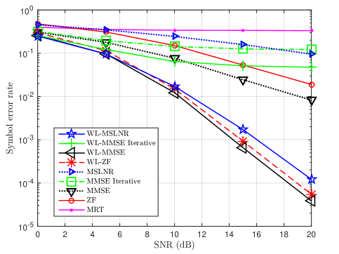
Figure 1: Average symbol error rates of users for $M=4$ transmit antennas and $K=4$ users with 4-PAM modulation. The MRT, ZF, and MMSE iterative precoding methods are given [17], MMSE precoding is given in [18], and MSLNR precoding is given in [20].

Fig. 1 compares the average symbol error rates of linear MRT, ZF, MMSE, iterative MMSE, and MSLNR precoding and their widely linear counterparts. As is expected, all the proposed widely linear precoding methods substantially outperform their linear counterparts. Moreover, it can be seen that the best performances are achieved by WL MMSE, WL ZF, and WL MSLNR. Maximum ratio transmission, which can be considered as both a linear and a widely linear processing technique, does not exhibit good performance in high SNRs, as expected. Similar to iterative MMSE [17], as SNR increases, iterative WL MMSE also reaches an error floor very soon and does not show a promising performance. Compared to MMSE, WL MMSE shows a gain of about 9.2 dB at the error probability of $8.25\times 10^{-3}$, which demonstrates substantial performance improvement of WL processing compared to that of linear processing. It is interesting to note that the high SNR and low SNR performances of the investigated linear precoding methods differ. At higher SNRs, the best performance is achieved from top to bottom by MMSE, ZF, MSLNR, iterative MMSE, and MRT. These results are consistent with the results obtained in [17]. In a similar fashion, if widely linear methods are compared to one another, at higher SNRs from best to worst the order of performance is WL MMSE, WL ZF, WL MSLNR, iterative WL MMSE, and MRT. An interesting remark on these comparisons is that widely linear processing substantially benefits MSLNR precoding. Linear MSLNR precoding, which in the above simulation setting did not perform well, significantly improved by using widely linear processing.

Figure 2: Average sum rates when $M=4$ and $K=2$ with 16-QAM modulated signals for ZF-QAM and MMSE-QAM and when $M=4$ and $K=4$ with 4-PAM modulated signals for the simulated widely linear precoding methods.

In Fig. 1, it was shown that widely linear precoding of one-dimensionally modulated signals outperforms linear precoding of one-dimensionally modulated signals. It would also be instructive to compare the performance of widely linear precoding of one-dimensionally modulated signals with that of linear precoding of two-dimensionally modulated signals. We use system throughput for this comparison. Fig. 2 depicts the expected sum rates of four users with 4-PAM modulation employing the proposed widely linear precoding methods and the sum rate of two users with 16-QAM modulation employing linear precoding methods. Theoretically, four users with 4-PAM modulation and two users with 16-QAM modulation, both achieve a maximum sum rate of 8 bits/channel use. Therefore, it is very interesting to observe that WL ZF and WL MMSE precoding of four 4-PAM modulated users outperform ZF and MMSE precoding of two 16-QAM modulated users. Widely linear MSLNR precoding also outperforms both ZF and MMSE precoding, at all simulated SNRs. The fact that iterative WL MMSE seems to be unable to achieve the sum rate of 8 bits/channel use is also consistent with our findings in Fig. 1 which exhibits the error floor of iterative WL MMSE precoding.

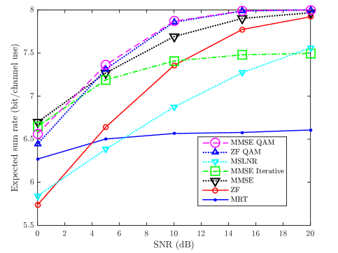
Figure 3: Average sum rates when $M=4$ and $K=2$ with 16-QAM modulated signals for ZF-QAM and MMSE-QAM and when $M=4$ and $K=4$ with 4-PAM modulated signals for the other simulated linear precoding methods.

To provide a more complete set of comparisons, we also present Fig. 3 which depicts the expected sum rates of linear precoding of four users with 4PAM modulation and ZF and MMSE precoding of two users with 16-QAM modulation. At high SNRs, the expected sum rates achieved by MMSE and ZF precoding of two 16-QAM modulated users is higher than any other combination of modulation and precoding, while at low SNRs, the expected sum rate of MMSE precoding of four 4-PAM modulated users is higher than any other combination of modulation and precoding. As expected from Fig. 1, MRT, iterative MMSE, and MSLNR precoding methods do not perform as well as other precoding methods. By comparing Figs. 2 and 3, it becomes clear that, at all simulated SNRs, all the proposed widely linear precoding methods achieve higher bit rates compared to their linear counterparts. This result is compatible with our findings in Fig. 1.

V-B User Selection

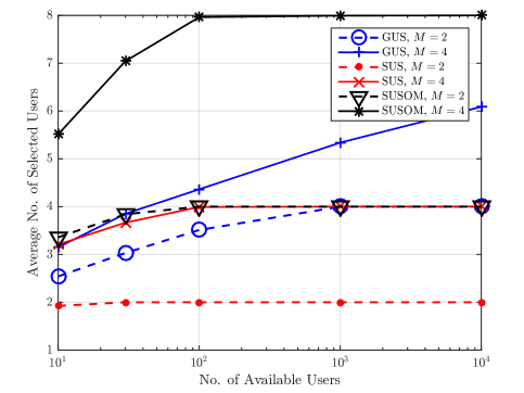
Figure 4: Average numbers of selected users with SUS [21], GUS [23], and SUSOM vs. total number of available users for $M=2,~{}4$ transmit antennas.

In this section, we evaluate the performance of the proposed SUSOM algorithm of Table II. In Fig. 4, the performance of SUSOM is compared to that of the SUS algorithm of [21] and the GUS algorithm of [23], for $M=2,4$ transmit antennas when one receive antenna is employed at each user. Each curve is averaged over 1,000 different channel realizations. It can be observed in Fig. 4 that as the number of available users increases, the number of selected users for all three algorithms increases until saturation. As can be seen, the SUS algorithm could select at most $M$ users for both cases of $M=2,~{}3$ antennas when $K$ is large enough. On the other hand, the proposed SUSOM algorithm can select up to at most $2M$ users, i.e., twice of that of the SUS algorithm. The GUS algorithm is also expected to saturate at $2M$ users, as it does for $M=2$ transmit antenna scenario. Nevertheless, it does not reach saturation in the scenario with $M=4$ transmit antennas even with up to 10,000 available users. This is an indication of the slow saturation rate of GUS with respect to the number of available users, which in turn indicates that GUS algorithm does not always find the best set of users compared to SUSOM, despite the fact that it can select more users than SUS. It is interesting to observe that even before saturation SUSOM outperforms both GUS and SUS. For example, when $M=4$ and there are only 10 users available, the average number of selected users is 5.51 with SUSOM, 3.15 with GUS, and 3.2 with SUS.

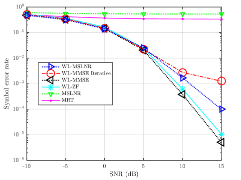
Figure 5: Average symbol error rates of users for $M=4$ and $K_{T}=100$ available users assuming the SUSOM algorithm is employed and all users transmit 4-PAM signals.

Fig. 5 compares the average symbol error rates of MRT, MSLNR, WL ZF, WL MMSE, iterative WL MMSE, and WL MSLNR precoding when the SUSOM algorithm is employed. It is assumed that at first the SUSOM algorithm selects a set of users out of $K_{T}=100$ available users and then the transmitter broadcasts information to the selected users using the above precoding methods. From Fig. 4 it is known that using SUSOM algorithm the average number of selected users is 7.96 when $K_{T}=100$, i.e., more than the number of transmit antennas (system is overloaded). Therefore, we do not perform linear ZF, MMSE, and iterative MMSE for these cases, since they are not designed to work on overloaded systems in their presented form. We also do not show the error probabilities of the above precoding methods combined with GUS and SUS algorithms, since GUS and SUS algorithms select different numbers of users compared to SUSOM, and therefore comparing the error probabilities in such a case would not bear a meaningful interpretation. However, if we compare Fig. 5 and Fig. 1, it can be observed that the SUSOM algorithm not only selects more users than that in Fig. 1, but also all the investigated precoding methods under SUSOM achieve a better symbol error rate compared to those of Fig. 1.

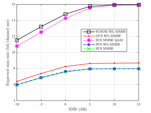
Figure 6: Average sum rates when $M=4$ and $K_{T}=100$ with 16-QAM modulated signals for SUS MMSE QAM and when $M=4$ and $K_{T}=100$ with 4-PAM modulated signals for the other user selection and precoding methods. The the MMSE precoding is given in [18], the SUS algorithm is given in [21], and the GUS algorithm is given in [23].

As observed in Fig. 5, since the error probability alone is not a good indicator of the performance when there are different numbers of users in the system, Fig. 6 is provided to gain more insight into the relative performances of the user selection algorithms. In Fig. 6, the expected sum rates of 4-PAM modulated users for combinations of SUS with MMSE, SUS with WL MMSE, GUS with WL MMSE, and SUSOM with WL MMSE are presented. In addition, the expected sum rate of 16-QAM modulated users with SUS algorithm and MMSE precoding is also plotted for comparison. As can be seen, at all simulated SNRs, the combination of SUSOM with 4-PAM and WL MMSE achieves the highest throughput. It can be seen in Fig. 6 that as SNR increases, the achievable expected throughput approaches limits determined by the average numbers of selected users and the order of modulation. For this example, at higher SNRs the achievable throughput of both SUSOM with 4-PAM and SUS with 16-QAM are 16 bits/channel use.

VI Conclusion

In this paper, we proposed a widely linear (WL) transmit precoding design for one-dimensionally modulated signals in a standard broadcast communications channel. Closed-form solutions for the precoders of the WL MRT and the WL ZF were obtained by using complex-domain analysis and closed-form solutions of WL MMSE and WL MSLNR were obtained by analysis of the composite real representation. It was shown that WL ZF and WL MMMSE precoders can properly operate even if the number of users is twice as large as the number of transmit antennas, as opposed to linear ZF and MMSE precoders which can only support as many users as the number of transmit antennas. We also developed a user selection algorithm, compatible with widely linear precoding, that can select twice as many users as the number of transmit antennas. It has been shown that WL precoding outperforms linear precoding. Moreover, it has been shown that widely linear precoding in conjunction with the proposed semi-orthogonal user selection algorithm for one-dimensional modulation (SUSOM) also outperforms linear precoding in conjunction with semi-orthogonal user selection algorithm (SUS).

[Proof of Claim 1] Let us consider the following isomorphism from the complex field to the real field:

$${\bf h}_{k}\in\mathbb{C}^{1\times M}\xrightarrow{\mathcal{T}_{1}}{\bf\bar{h}}_{k}=\left[\begin{array}[]{cc}\Re\{{\bf h}_{k}\}&\Im\{{\bf h}_{k}\}\end{array}\right]\in\mathbb{R}^{1\times 2M},$$ (52)

$$1\leq k\leq K.$$ (53)

Then, it is obvious that

$$\Re\{{\bf h}_{k}{\bf h}_{j}^{H}\}={\bf\bar{h}}_{k}{\bf\bar{h}}_{j}^{T}.$$ (54)

If we define the $K\times 2M$ matrix ${\bf\bar{H}}$ as

$${\bf\bar{H}}=\left[\begin{array}[]{c}{\bf\bar{h}}_{1}\\ \vdots\\ {\bf\bar{h}}_{K}\end{array}\right],$$ (55)

then we have the following lemma:

Lemma 1

All $K$ channels are mutually orthogonal if and only if the $K\times K$ matrix ${\bf\bar{H}}{\bf\bar{H}}^{T}$ is a full rank diagonal matrix.

Proof:

If ${\bf\bar{H}}{\bf\bar{H}}^{T}$ is a full rank diagonal matrix, then it is equivalently represented by $\operatorname{diag}(\allowbreak\|{\bf\bar{h}}_{1}\|_{2}^{2},\ldots,\|{\bf\bar{h}}_{K}\|_{2}^{2})$. In other words, ${\bf\bar{h}}_{k}{\bf\bar{h}}_{j}^{T}=0$, $1\leq j\neq k\leq K$, i.e., the channels are mutually orthogonal. On the other hand, $\|{\bf\bar{h}}_{k}\|_{2}\neq 0$ with probability one and if the channels are mutually orthogonal then ${\bf\bar{h}}_{k}{\bf\bar{h}}_{j}^{T}=0$, $1\leq j\neq k\leq K$, which results in ${\bf\bar{H}}{\bf\bar{H}}^{T}$ being a full rank diagonal matrix. ∎

On the other hand, it is known that $\operatorname{rank}({\bf\bar{H}}{\bf\bar{H}}^{T})=\operatorname{rank}({\bf\bar{H}})\leq\min(K,2M)\leq 2M$. Therefore, the maximum number of mutually orthogonal channels is $K=2M$.

References

- [1] W. Brown and R. Crane, “Conjugate linear filtering,” IEEE Trans. Inf. Theory, vol. 15, no. 4, pp. 462–465, Jul. 1969.
- [2] B. Picinbono and P. Chevalier, “Widely linear estimation with complex data,” IEEE Trans. Signal Process., vol. 43, no. 8, pp. 2030–2033, Aug. 1995.
- [3] C. Hellings, M. Joham, and W. Utschick, “QoS feasibility in MIMO broadcast channels with widely linear transceivers,” IEEE Signal Process. Lett., vol. 20, no. 11, pp. 1134–1137, Nov. 2013.
- [4] M. Bavand and S. D. Blostein, “Widely linear multiuser simultaneous information and power transfer with one-dimensional signaling,” in Proc. IEEE GLOBECOM Workshops, DC, Dec. 2016 (in press).
- [5] C. Perera, A. Zaslavsky, P. Christen, and D. Georgakopoulos, “Context aware computing for the Internet of things: A survey,” IEEE Commun. Surveys Tuts., vol. 16, no. 1, pp. 414–454, 2014.
- [6] “LTE-M - optimizing LTE for the Internet of things,” Nokia Network White Paper, 2015.
- [7] A. Pantelopoulos and N. G. Bourbakis, “A survey on wearable sensor-based systems for health monitoring and prognosis,” IEEE Trans. Syst., Man, Cybern. C, vol. 40, no. 1, Jan. 2010.
- [8] M. Patel and J. Wang, “Applications, challenges, and prospective in emerging body area networking technologies,” IEEE Wireless Commun., vol. 17, no. 1, pp. 80–88, Feb. 2010.
- [9] “Emerging communication technologies enabling the Internet of things,” Rohde & Schwarz White Paper, Sep. 2016.
- [10] T. McWhorter and P. Schreier, “Widely-linear beamforming,” in Proc. Asilomar Conf. Signals, Syst. Comput., Nov. 2003, pp. 753–759.
- [11] P. Chevalier and F. Pipon, “New insights into optimal widely linear array receivers for the demodulation of BPSK, MSK, and GMSK signals corrupted by noncircular interferences-application to SAIC,” IEEE Trans. Signal Process., vol. 54, no. 3, pp. 870–883, Mar. 2006.
- [12] P. Chevalier, J.-P. Delmas, and A. Oukaci, “Optimal widely linear MVDR beamforming for noncircular signals,” in Proc. IEEE Int. Conf. Acoust., Speech, Signal Process. (ICASSP), 2009, pp. 3573–3576.
- [13] S. Tan, L. Xu, S. Chen, and L. Hanzo, “Iterative soft interference cancellation aided minimum bit error rate uplink receiver beamforming,” in Proc. 63rd IEEE Veh. Technol. Conf. (VTC).
- [14] Y. Zeng, C. M. Yetis, E. Gunawan, Y. L. Guan, , and R. Zhang, “Transmit optimization with improper Gaussian signaling for interference channels,” IEEE Trans. Signal Process., vol. 61, no. 11, pp. 2899–2913, Jun. 2013.
- [15] P. Xiao and M. Sellathurai, “Improved linear transmit processing for single-user and multi-user MIMO communications systems,” IEEE Trans. Signal Process., vol. 58, no. 3, pp. 1768–1779, Mar. 2010.
- [16] S. Huang, H. Yin, J. Wu, and V. C. M. Leung, “User selection for multiuser MIMO downlink with zero-forcing beamforming,” IEEE Trans. Veh. Technol., vol. 62, no. 7, pp. 3084–3097, Sep. 2013.
- [17] M. Joham, W. Utschick, and J. A. Nossek, “Linear transmit processing in MIMO communications systems,” IEEE Trans. Signal Process., vol. 53, no. 8, pp. 2700–2712, Aug. 2005.
- [18] C. B. Peel, B. M. Hochwald, and A. L. Swindlehurst, “A vector-perturbation technique for near-capacity multiantenna multiuser communication-part I: Channel inversion and regularization,” IEEE Trans. Commun., vol. 53, no. 1, pp. 195–202, Jan. 2005.
- [19] S. Serbetli and A. Yener, “Transceiver optimization for multiuser MIMO systems,” IEEE Trans. Signal Process., vol. 52, no. 1, pp. 214–226, Jan. 2004.
- [20] M. Sadek, A. Tarighat, and A. H. Sayed, “A leakage-based precoding scheme for downlink multi-user MIMO channels,” IEEE Trans. Wireless Commun., vol. 6, no. 5, pp. 1711–1721, May 2007.
- [21] T. Yoo and A. Goldsmith, “On the optimality of multiantenna broadcast scheduling using zero-forcing beamforming,” IEEE J. Sel. Areas Commun., vol. 24, no. 3, pp. 528–541, Mar. 2006.
- [22] Z. Shen, R. Chen, J. G. Andrews, R. W. Heath Jr., and B. L. Evans, “Low complexity user selection algorithms for multiuser MIMO systems with block diagonalization,” IEEE Trans. Signal Process., vol. 54, no. 9, pp. 3658–3663, Sep. 2006.
- [23] M. Bavand and S. D. Blostein, “Modulation-specific multiuser transmit precoding and user selection for BPSK signalling,” arXiv:1603.04812 [cs.IT], Oct. 2016.
- [24] A. Paulraj, R. Nabar, and D. Gore, Introduction to Space-Time Wireless Communications. Cambridge University Press, 2003.
- [25] J. Mao, J. Gao, Y. Liu, and G. Xie, “Simplified semi-orthogonal user selection for MU-MIMO systems with ZFBF,” IEEE Wireless Commun. Lett., vol. 1, no. 1, pp. 42–45, Feb. 2012.
- [26] F. D. Neeser and J. L. Massey, “Proper complex random processes with applications to information theory,” IEEE Trans. Inf. Theory, vol. 39, no. 4, pp. 1293–1302, Jul. 1993.
- [27] J. G. Proakis, Digital Communications, 4th ed. McGraw-Hill, 2001.
- [28] E. Bjornson, M. Bengtsson, and B. Ottersten, “Optimal multiuser transmit beamforming: A difficult problem with a simple solution structure,” IEEE Signal Process. Mag., vol. 31, no. 4, pp. 142–148, Jul. 2014.
- [29] D. Brandwood, “A complex gradient operator and its application in adaptive array theory,” Proc. IEEE, vol. 130, no. 1, pp. 11–16, Feb. 1983.
- [30] A. Hjørungnes and D. Gesbert, “Complex-valued matrix differentiation: Techniques and key results,” IEEE Trans. Signal Process., vol. 55, no. 6, pp. 2740–2746, Jun. 2007.
- [31] J. Eriksson, E. Ollila, and V. Koivunen, “Essential statistics and tools for complex random variables,” IEEE Trans. Signal Process., vol. 58, no. 10, pp. 5400–5408, Oct. 2010.
- [32] J. Nocedal and S. J. Wright, Numerical Optimization, 2nd ed. New York, USA: Springer, 2006.
- [33] S. Boyd, N. Parikh, E. Chu, B. Peleato, and J. Eckstein, Distributed Optimization and Statistical Learning via the Alternating Direction Method of Multipliers. Now, 2011.
- [34] W. Yu and R. Lui, “Dual methods for nonconvex spectrum optimization of multicarrier systems,” IEEE Trans. Commun., vol. 54, no. 7, pp. 1310–1322, Jul. 2006.
- [35] N. Mokari, M. R. Javan, and K. Navaie, “Cross-layered resource allocation in OFDMA systems for heterogenous trafic with imperfect CSI,” IEEE Trans. Veh. Technol., vol. 59, no. 2, pp. 1011–1017, Feb. 2010.
- [36] T. K. Moon and W. C. Stirling, Mathematical Methods and Algorithms for Signal Processing. Prentice Hall, 1999.
- [37] A. Wiesel, Y. C. Eldar, and S. Shamai, “Linear precoding via conic optimization for fixed MIMO receivers,” IEEE Trans. Signal Process., vol. 54, no. 1, pp. 161–176, Jan. 2006.
- [38] M. Schubert and H. Boche, “Solution of the multiuser downlink beamforming problem with individual SINR constraints,” IEEE Trans. Veh. Technol., vol. 53, no. 1, pp. 18–28, Jan. 2004.
- [39] Q. H. Spencer, A. L. Swindlehurst, and M. Haardt, “Zero-forcing methods for downlink spatial multiplexing in multiuser MIMO channels,” IEEE Trans. Signal Process., vol. 52, no. 2, pp. 461–471, Feb. 2004.
- [40] J. Grob, G. Trenkler, and S.-O. Troschke, “On semi-orthogonality and special class of matrices,” Linear Algebra and its Applications, vol. 289, pp. 169–182, Mar. 1999.
- [41] A. Barg and D. Y. Nogin, “Bounds on packings of spheres in the Grassmann manifold,” IEEE Trans. Inf. Theory, vol. 48, no. 9, pp. 2450–2454, Sep. 2002.