A Central Limit Theorem for an Omnibus Embedding of Multiple Random Graphs and Implications for Multiscale Network Inference

Abstract

Performing statistical analyses on collections of graphs is of import to many disciplines, but principled, scalable methods for multi-sample graph inference are few. Here we describe an “omnibus” embedding in which multiple graphs on the same vertex set are jointly embedded into a single space with a distinct representation for each graph. We prove a central limit theorem for this embedding and demonstrate how it streamlines graph comparison, obviating the need for pairwise subspace alignments. The omnibus embedding achieves near-optimal inference accuracy when graphs arise from a common distribution and yet retains discriminatory power as a test procedure for the comparison of different graphs. Moreover, this joint embedding and the accompanying central limit theorem are important for answering multiscale graph inference questions, such as the identification of specific subgraphs or vertices responsible for similarity or difference across networks. We illustrate this with a pair of analyses of connectome data derived from dMRI and fMRI scans of human subjects. In particular, we show that this embedding allows the identification of specific brain regions associated with population-level differences. Finally, we sketch how the omnibus embedding can be used to address pressing open problems, both theoretical and practical, in multisample graph inference.

Keywords: multiscale graph inference, graph embedding, multiple-graph hypothesis testing

1 Introduction

Statistical inference across multiple graphs is of vital interdisciplinary interest in domains as varied as machine learning, neuroscience, and epidemiology. Inference on random graphs frequently depends on appropriate low-dimensional Euclidean representations of the vertices of these graphs, known as graph embeddings, typically given by spectral decompositions of adjacency or Laplacian matrices (Belkin and Niyogi, 2003; Sussman et al., 2012; Chatterjee, 2015). Nonetheless, while spectral methods for parametric inference in a single graph are well-studied, multi-sample graph inference is a nascent field. See, for example, the authors’ work in (Tang et al., 2017a, b) as among the only principled approaches to two-sample graph testing. What is more, for inference tasks involving multiple graphs—for instance, determining whether two or more graphs on the same vertex set are similar—discerning an optimal simultaneous embedding for all graphs is a challenge: how can such an embedding be structured to both provide estimation accuracy of common parameters when the graphs are similar, but retain discriminatory power when they are different?

A flexible, robust embedding procedure to achieve both goals would be of considerable utility in a range of real data applications. For instance, consider the problem of community detection in large networks. While algorithms for community detection abound, relatively few approaches exist to address community classification; that is, to leverage graph structure to successfully establish which subcommunities appear statistically similar or different. In fact, the authors’ work in Lyzinski et al. (2017) represents one of the earliest forays into statistically principled techniques for subgraph classification in hierarchical networks. Not surprisingly, the creation of a graph-statistical analogue of the classical analysis-of-variance $F$-test, in which a single test procedure would permit the comparison of graphs from multiple populations, is very much an open problem of immediate import. But even given a coherent framework for extracting graph-level differences across multiple populations of graphs, there remains the further complication of replicating this at multiple scales, by isolating—in the spirit of post-hoc tests such as Tukey’s studentized range—precisely which subgraphs or vertices in a collection of vertex-matched graphs might be most similar or different.

Our goal in this paper, then, is to provide a unified framework to answer the following questions:

1. Given a collection of random graphs, can we develop a single statistical procedure that accurately estimates common underlying graph parameters, in the case when these parameters are equal across graphs, but also delivers meaningful power for testing when these graph parameters are distinct?

2. Can we develop an inference procedure that identifies sources of graph similarity or difference at scales ranging from whole-graph to subgraph to vertex? For example, can we identify particular vertices that contribute significantly to statistical differences at the whole-graph level?

3. Can we develop an inference procedure that scales well to large graphs, addresses graphs that are weighted, directed, or whose edge information is corrupted, and which is amenable to downstream classical statistical methodology for Euclidean data?

4. Does such a statistical procedure compare favorably to existing state-of-the-art techniques for joint graph estimation and testing, and does it work well on real data?

Here, we address each of these open problems with a single embedding procedure. Specifically, we describe an omnibus embedding, in which the adjacency matrices of multiple graphs on the same vertex-matched set are jointly embedded into a single space with a distinct representation for each graph and, indeed, each vertex of each graph. We then prove a central limit theorem for this embedding, a limit theorem similar in spirit to, but requiring a significantly more delicate probabilistic analysis than, the one proved in Athreya et al. (2016). We show, in both simulated and real data, that the asymptotic normality of these embedded vertices has demonstrable utility. First, the omnibus embedding performs nearly optimally for the recovery of graph parameters when the graphs are from the same distribution, but compares favorably with state-of-the-art hypothesis testing procedures to discern whether graphs are different. Second, the simultaneous embedding into a shared space allows for the comparison of graphs without the need to perform pairwise alignments of the embeddings of different graphs. Third, the asymptotic normality of the omnibus embedding permits the application of a wide array of subsequent Euclidean inference techniques, most notably a multivariate analysis of variance (MANOVA) to isolate statistically significant vertices across several graphs. Thus, the omnibus embedding provides a statistically sound analogue of a post-hoc Tukey test for multisample graph inference. We demonstrate this with an analysis of real data, comparing a collection of magnetic resonance imaging (MRI) scans of human brains to identify dissimilar graphs and then to further pinpoint specific intra-graph features that account for global graph differences.

The main theoretical results of this paper are a consistency theorem for the omnibus embedding, akin to Lyzinski et al. (2014), and a central limit theorem, akin to Athreya et al. (2016), for the distribution of any finite collection of rows of this omnibus embedding. We emphasize that distributional results for spectral decompositions of random graphs are few. The classic results of Füredi and Komlós (1981) describe the eigenvalues of the Erdős-Rényi random graph and the work of Tao and Vu (2012) concerns distributions of eigenvectors of more general random matrices under moment restrictions, but Athreya et al. (2016) and Tang and Priebe (2018) are among the only references for central limit theorems for spectral decompositions of adjacency and Laplacian matrices for a class of independent-edge random graphs broader than the Erdős-Rényi model.

Our consistency result shows that the omnibus embedding provides consistent estimates of certain unobserved vectors, called latent positions, that are associated to vertices of the graphs. At present, the best available spectral estimates of such latent positions involve averaging across graphs followed by an embedding, resulting in a single set of estimated latent positions, rather than in a distinct set for each graph. We find in simulations, that our omnibus-derived estimates perform competitively with these existing spectral estimates of the latent positions, while still retaining graph-specific information. In addition, we show that the omnibus embedding allows for a test statistic that improves on the state-of-the-art two-sample test procedure presented in Tang et al. (2017a) for determining whether two random dot product graphs (Young and Scheinerman, 2007) have the same latent positions.

Specifically, Tang et al. (2017a) introduces a test statistic generated by performing a Euclidean, lower-dimensional embedding of the graph adjacency matrix (see Sussman et al., 2012) of each of the two networks, followed by a Procrustes alignment (Gower, 1975; Dryden and Mardia, 1998) of the two embeddings. Addressing the nonparametric analogue of this question—whether two graphs have the same latent position distribution—is the focus of Tang et al. (2017b), which uses the embeddings of each graph to estimate associated density functions. The Procrustes alignment required by Tang et al. (2017b) both complicates the test statistic and, empirically, weakens the power of the test (see Section 5). Furthermore, it is unclear how to effectively adapt pairwise Procrustes alignments to tests involving more than two graphs. The omnibus embedding allows us to avoid these issues altogether by providing a multiple-graph representation that is well-suited to both latent position estimation and comparative graph inference methods.

Our paper is organized as follows. In Sec. 2, we give an overview of our main results and present two real-data examples in which the omnibus embedding uncovers important multiscale information in collections of brain networks. In Sec. 3, we present background information and formal definitions. In Sec. 4, we provide detailed statements of our principal theoretical results. In Sec. 5, we present simulation data that illustrates the power of the omnibus embedding as a tool for both estimation and testing. In our Supplementary Material, we provide detailed proofs, including a sharpening of a vertex-exchangeability argument for bounding residual terms in the difference between omnibus estimates and true graph parameter values. We conclude with a discussion of extensions and open problems on multi-sample graph inference.

2 Summary of main results and applications to real data

Recall that our goal is to develop a single spectral embedding technique for multiple-graph samples that (a) estimates common graph parameters, (b) retains discriminatory power for multisample graph hypothesis testing and (c) allows for a principled approach to identifying specific vertices that drive graph similarities or differences. In this section, we give an informal description of the omnibus embedding and a pared-down statement of our central limit theorem for this embedding, keeping notation to a minimum. We then demonstrate immediate payoffs in exploratory data analysis, leaving a more detailed technical descriptions of the method and our results for later sections.

To provide a theoretically-principled paradigm for graph inference for stochastically-varying networks, we focus on a particular class of random graphs. We define a graph $G$ to be an ordered pair of $(V,\mathcal{E})$ where $V$ is the vertex or node set, and $\mathcal{E}$, the set of edges, is a subset of the Cartesian product of $V\times V$. In a graph whose vertex set has cardinality $n$, we will usually represent $V$ as $V=\{1,2,\dots,n\}$, and we say there is an edge between $i$ and $j$ if $(i,j)\in\mathcal{E}$. The adjacency matrix $\mathbf{A}$ provides a representation of such a graph:

$$\mathbf{A}_{ij}=1\textrm{ if }(i,j)\in\mathcal{E},\textrm{ and }\mathbf{A}_{ij}=0\textrm{ otherwise. }$$

Where there is no danger of confusion, we will often refer to a graph $G$ and its adjacency matrix $\mathbf{A}$ interchangeably.

Any model of a stochastic network must describe the probabilistic mechanism of connections between vertices. We focus on a class of latent position random graphs Hoff et al. (2002); Diaconis and Janson (2008); Smith et al. (2017),in which every vertex has associated to it a (typically unobserved) latent position, itself an object belonging to some (often Euclidean) space $\mathcal{X}$. Probabilities of an edge between two vertices $i$ and $j$, $p_{ij}$, are a function $\kappa(\cdot,\cdot):\mathcal{X}\times\mathcal{X}\rightarrow[0,1]$ (known as the link function) of their associated latent positions $(x_{i},x_{j})$. Thus $p_{ij}=\kappa(x_{i},x_{j})$, and given these probabilities, the entries $\mathbf{A}_{ij}$ of the adjacency matrix $\mathbf{A}$ are independent Bernoulli random variables with success probabilities $p_{ij}$. We consolidate these probabilities into a matrix $\mathbf{P}=(p_{ij})$, and write $\mathbf{A}\sim\mathbf{P}$ to denote this relationship.

The latent position graph model has tremendous utility in modeling natural phenomena. For example, individuals in a disease network may have a hidden vector of attributes (prior illness, high-risk occupation) that observers of disease dynamics do not see, but which nevertheless strongly influence the chance that such an individual may become ill or infect others. Because the link function is relatively unrestricted, latent position models can replicate a wide array of graph phenomena (Olhede and Wolfe, 2014).

In a $d$-dimensional random dot product graph (Young and Scheinerman, 2007), the latent space is an appropriately-constrained subspace of $\mathbb{R}^{d}$, and the link function is simply the dot product of the two latent $d$-dimensional vectors. The invariance of the inner product to orthogonal transformations is a nonidentifiability in the model, so we frequently specify accuracy up to a rotation matrix $\mathbf{W}$. Random dot product graphs are often divided into two types: those in which the latent positions are fixed, and those in which the latent positions are themselves random. We will address both cases here: in our theoretical results, the latent positions $X_{i}\in\mathbb{R}^{d}$ for vertex $i$ are drawn independently from a common distribution $F$ on $\mathbb{R}^{d}$; and our practical applications, we consider how to use an omnibus embedding to address the question of equality of potentially non-random latent positions. For the case in which the latent positions are drawn at random from some distribution $F$, an important graph inference task is the inference of properties of $F$ from an observation of the graph alone. In the graph inference setting, there is both randomness in the latent positions, and given these latent positions, a subsequent conditional randomness in the existence of edges between vertices. A key to inference in such models is the initial step of consistently estimating the unobserved $X_{i}$’s from a spectral decomposition of $\mathbf{A}$, and then using these estimates, denoted $\hat{X}_{i}$, to infer properties of $F$.

For an RDPG with $n$ vertices, the $n\times d$ matrix of latent positions $\mathbf{X}$ is formed by taking vector $\mathbf{X}_{i}$ associated to vertex $i$ to be the $i$-th row of $\mathbf{X}$. Then $\mathbf{P}=[p_{ij}]$, the matrix of probabilities of edges between vertices, is easily expressed as $\mathbf{P}=\mathbf{X}\mathbf{X}^{T}$. The aforementioned nonidentifiability is now transparent: if $\mathbf{W}$ is orthogonal, then $\mathbf{X}\mathbf{W}\mathbf{W}^{T}\mathbf{X}^{T}=\mathbf{P}$ as well, so the rotated latent positions $\mathbf{X}\mathbf{W}$ generate the same the matrix of probabilities. Given such a model, a natural inference task is that of estimating the latent position matrix $\mathbf{X}$ up to some orthogonal transformation.

Because of the assumption that the matrix $\mathbf{P}$ is of comparatively low rank, random dot product graphs can be analyzed with a number of tools from classical linear algebra, such as singular-value decompositions of their adjacency matrices. Nevertheless, this tractability does not compromise the utility of the model. Random dot product graphs are flexible enough to approximate a wide class of independent-edge random graphs (Tang et al., 2013), including the stochastic block model (Holland et al., 1983; Karrer and Newman, 2011).

Under mild assumptions, the adjacency matrix $\mathbf{A}$ of a random dot product graph is a rough approximation of the matrix $\mathbf{P}=[p_{ij}]$ of edge probabilities in the sense that the spectral norm of $\mathbf{A}-\mathbf{P}$ can be controlled; see for example Oliveira (2009) and Lu and Peng (2013). In Sussman et al. (2012), Sussman et al. (2012) and Lyzinski et al. (2014), it is established that, under eigengap assumptions on $\mathbf{P}$, a partial spectral decomposition of the adjacency matrix $\mathbf{A}$, known as the adjacency spectral embedding (ASE), allows for consistent estimation of the true, unobserved latent positions $\mathbf{X}$. That is, if we define $\hat{\mathbf{X}}=\mathbf{U}_{\mathbf{A}}\mathbf{S}_{\mathbf{A}}^{1/2}$, where $\mathbf{S}_{\mathbf{A}}$ is the diagonal matrix of the top $d$ eigenvalues of $A$, sorted by magnitude, and if $\mathbf{U}_{\mathbf{A}}$ are the associated unit eigenvectors, then the rows of this truncated eigendecomposition of $\mathbf{A}$ are consistent estimates $\{\hat{\mathbf{X}}_{i}\}$ of the latent positions $\{\mathbf{X}_{i}\}$. Of course, these latent positions are often the parameters we wish to estimate. In Lyzinski et al. (2017), it is shown that embedding the adjacency matrix and then performing a novel angle-based clustering of the rows is key to decomposing large, hierarchical networks into structurally similar subcommunities. In Athreya et al. (2016), it is shown that the suitably-scaled eigenvectors of the adjacency matrix converge in distribution to a Gaussian mixture. In this paper, we prove a similar result for an omnibus matrix generated from multiple independent graphs.

The ASE provides a consistent estimate for the true latent positions in a random dot product graph up to orthogonal transformations. Hence a Procrustes distance between the adjacency spectral embedding of two graphs on the same vertex set serves as a test statistic for determining whether two random dot product graphs have the same latent positions (Tang et al., 2017a). Specifically, let $\mathbf{A}^{(1)}$ and $\mathbf{A}^{(2)}$ be the adjacency matrices of two random dot product graphs on the same vertex set (with known vertex correspondence), and let $\hat{\mathbf{X}}$ and $\hat{\mathbf{Y}}$ be their respective adjacency spectral embeddings. If the two graphs have the same generating $\mathbf{P}$ matrices, it is reasonable to surmise that the Procrustes distance

$$\min_{\mathbf{W}\in\mathcal{O}^{d\times d}}\|\hat{\mathbf{X}}-\hat{\mathbf{Y}}\mathbf{W}\|_{F},$$ (1)

where $\|\cdot\|_{F}$ denotes the Frobenius norm of a matrix, will be relatively small. In Tang et al. (2017a), the authors show that a scaled version of the Procrustes distance in (1) provides a valid and consistent test for the equality of latent positions for a pair of random dot product graphs. Unfortunately, the fact that a Procrustes minimization must be performed both complicates the test statistic and compromises its power.

Here, we instead consider an embedding of an omnibus matrix, defined as follows. Given two independent $d$-dimensional RDPG adjacency matrices $\mathbf{A}^{(1)}$ and $\mathbf{A}^{(2)}$, on the same vertex set with known vertex correspondence, the omnibus matrix $\mathbf{M}$ is given by

$$\mathbf{M}=\begin{bmatrix}\mathbf{A}^{(1)}&\frac{\mathbf{A}^{(1)}+\mathbf{A}^{(2)}}{2}\\ \frac{\mathbf{A}^{(1)}+\mathbf{A}^{(2)}}{2}&\mathbf{A}^{(2)}\end{bmatrix},$$ (2)

Note that this matrix easily extends to a sequence of graphs $\mathbf{A}^{(1)},\cdots,\mathbf{A}^{(m)}$, where the block diagonal entries are the matrices $\mathbf{A}^{(i)}$ and the $(l,k)$-th off-diagonal block is the matrix $\frac{\mathbf{A}^{(k)}+\mathbf{A}^{(l)}}{2}$.

Analogously to our notation for the adjacency spectral embedding $\hat{\mathbf{X}}$, let $\mathbf{S}_{\mathbf{M}}$ represent the $d\times d$ matrix of top $d$ eigenvalues of $\mathbf{M}$, ordered again by magnitude, and let $\mathbf{U}_{\mathbf{M}}$ be the $mn\times d$-dimensional matrix of associated eigenvectors. Define the omnibus embedding, denoted $\textrm{OMNI}(\mathbf{M})$, by $\mathbf{U}_{\mathbf{M}}\mathbf{S}_{\mathbf{M}}^{1/2}$. We stress that $\textrm{OMNI}(\mathbf{M})$ produces $m$ separate points in Euclidean for each graph vertex—effectively, one such point for each copy of the multiple graphs in our sample. This property renders the omnibus embedding useful for all manner of post-hoc inference.

If we consider the rows of the omnibus embedding as potential estimates for the latent positions, two immediate questions are arise. Are these estimates consistent, and can we describe a scaled limiting distribution for them as graph size increases? We answer both of these in the affirmative.

Key result 1: The rows of the omnibus embedding provide consistent estimates for graph latent positions. If the latent positions of the graphs $\mathbf{A}^{(1)},\cdots,\mathbf{A}^{m}$ are equal, then under mild assumptions, the rows of $\textrm{OMNI}(\mathbf{M})$ provide consistent estimates of their corresponding latent positions. Specifically, if $h=n(s-1)+i$, where $1\leq i\leq n$ and $1\leq s\leq m$, then there exists an orthogonal matrix $\mathbf{W}$ such that

$$\max_{1\leq i\leq n}\|(\mathbf{U}_{\mathbf{M}}\mathbf{S}_{\mathbf{M}}^{1/2})_{h}-\mathbf{W}\mathbf{X}_{i}\|<\frac{C\log mn}{\sqrt{n}}$$

with high probability. This consistency result is especially useful because it bounds the error between true and estimated latent positions for all latent positions simultaneously. It further guarantees that the omnibus embedding competes well against the current best-performing estimator of the common latent positions $\mathbf{X}$, which is the adjacency spectral embedding of the sample mean matrix $\bar{\mathbf{A}}=\frac{\sum_{i=1}^{m}\mathbf{A}^{(i)}}{m}$ (Tang et al., 2016). Thus, the omnibus embedding is not just consistent when the latent positions are equal; it is close to near-optimal, and we exhibit this clearly in simulations (see Sec. 5).

Our second key result concerns the limiting distribution, as the graph size $n$ increases, of the rows of the omnibus embedding in the case when the graphs are independent and have the same latent positions.

Key result 2: For large graphs, the scaled rows of the omnibus embedding are asymptotically normal. Suppose that the latent positions for each graph are drawn i.i.d from a suitable distribution $F$, and that conditional on these latent positions, the adjacency matrices $\mathbf{A}^{(1)},\cdots,\mathbf{A}^{(m)}$ are independent realizations of random dot product graphs with the given latent positions. Let $\mathbf{Z}$ represent that $mn\times d$ dimensional matrix of latent positions for the graphs. Let $h=n(s-1)+i$, where $1\leq i\leq n$ and $1\leq s\leq m-1$. Then under mild assumptions, there exists a sequence of orthogonal matrices $\mathbf{W}_{n}$ such that as $n\rightarrow\infty$,

$$\sqrt{n}[(\mathbf{U}_{\mathbf{M}}\mathbf{S}_{\mathbf{M}}^{1/2})\mathbf{W}_{n}-\mathbf{Z}]_{h}$$

converges to a mean-zero $d$-dimensional Gaussian mixture. Hence the omnibus embedding allows for accurate estimation when the latent positions are equal; provides multiple points for each vertex; and under mild assumptions on the structure of the latent positions, these embeddings are approximately normal for large graph sizes. Even more remarkably, for testing whether two graphs have the same latent positions, we can build the omnibus embedding and consider only the Frobenius norm of the difference between the matrices defined by, respectively, the first $n$ and the second $n$ rows of this decomposition. This matrix difference, without any further Procrustes alignment, also serves as a test statistic for the equality of latent positions, which brings us to our third point.

Key simulation evidence: The omnibus embedding has meaningful power for two- and multi-sample graph hypothesis testing. The omnibus embedding, without subsequent Procrustes alignments, yields an improvement in power over state-of-the-art methods in two-graph testing, as borne out by a comparison on simulated data. Combined with our earlier bounds on the $2\to\infty$-norm difference between true and estimated latent positions, this demonstrates that the omnibus embedding provides estimation accuracy when the graphs are drawn from the same latent positions and improved discriminatory power when they are different. What is more, the omnibus embedding produces multiple points for each vertex and our asymptotic normality guarantees that these points are approximately normal. As a consequence, the omnibus embedding not only permits the discovery of graph-wide differences, but also the isolation of vertices that contribute to these differences, via, for instance, a multivariate analysis of variance (MANOVA) applied to these embedded vectors. This leads us to our final point.

Key real data analysis: the omnibus embedding isolates graph-wide differences and gives principled evidence for vertex significance in those differences, and works well on complicated real data. On weighted, directed, noisily-observed real graphs, slight modifications to the omnibus embedding procedure yield genuine exploratory insights into graph structure and vertex importance, with actionable import in application domains.

To demonstrate this, we present in the next subsections detailed analyses of two neuroscientific data sets. The first is a connectomic data set, in which we analyze a collection of paired diffusion MRI (dMRI) brain scans across 57 patients (Kiar, 2018), a comparison of 114 graphs with 172 common vertices. Second, we consider the COBRE data set (Aine et al., 2017), a collection of functional MRI scans of $54$ schizophrenic patients and $69$ healthy controls, with each scan yielding a graph on $264$ common vertices. In both data sets, we show how the omnibus embeddings can identify whole-graph differences as well as particular vertices involved in this difference.

2.1 Discerning vertex-level difference in paired brain scans of human subjects

As a case study in the utility of our techniques, we consider data from human brain scans collected on 57 subjects at Beijing Normal University. The data, labeled “BNU1”, is available at
http://fcon_1000.projects.nitrc.org/indi/CoRR/html/bnu_1.html.

This diffusion MRI data comprises two scans on each of 57 different patients, for a total of 114 scans. The dMRI data was converted into weighted graphs via the Neuro-Data-MRI-to-Graphs (NDMG) pipeline of Kiar (2018), with vertices representing sub-regions defined via spatial proximity and edges by tensor-based fiber streamlines connecting these regions. As such, by condensing vertices in a given brain region still further, neuroscientists can represent this data at different scales. We focus on data at a resolution in which the $m=114$ graphs have $n=172$ common vertices. (We point out that in Priebe et al. (To appear), this same data, at slightly different scale, serves as a useful illustration of different structural properties uncovered by different spectral embeddings). Our inference goals are to determine which of these graphs appear statistically similar and to elucidate which vertices might be key contributors to such difference.

We binarize the graphs via a simple thresholding operation, replacing all nonzero edge weights with 1, and leaving unchanged edges of weight zero. For reference, Figure 1 shows a visualization of one pair of adjacency matrices. Alternative approaches to weighted graphs, such as a replacement of weights by a rank-ordering, are also possible and have proven useful (see Priebe et al., To appear), but we do not pursue this here.

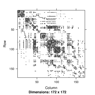
(a)

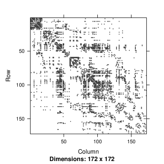
(b)

Figure 1: Binarized adjacency matrices for two BNU-1 brain graphs

With these $m=114$ binarized, undirected adjacency matrices, we generate the $m$-fold omnibus matrix $M$, the $m$-fold analogue of the matrix in Eq. (2), which is of size $(114\times 172)\times(114\times 172)$. To select a dimension for the omnibus embedding, we apply the profile-likelihood method of Zhu and Ghodsi (2006) to $M$. This procedure performs model selection (i.e., estimates the rank of $\mathbb{E}M$) by locating an elbow in the screeplot of the eigenvalues of $M$ (shown in Figure 2(a)) This yields an estimated embedding dimension of $\hat{d}=10$. As a check, we perform the same estimation procedure on all of the 114 graphs as well. Reassuringly, we recover an estimated embedding dimension close to $10$ for almost all of them, and proceed with $\hat{d}=10$, as summarized by the boxplot in Fig. 2(b).

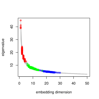
(a)

(b)

Figure 2: (a) Eigenvalues and embedding dimension for the omnibus matrix as BNU data. Note the second elbow at $\hat{d}=10$. (b) Box plot of the first three elbows in the scree plot identified by the profile-likelihood method of Zhu and Ghodsi (2006) applied to the 114 brain graphs individually. Note that the second elbow is concentrated around $\hat{d}=10$.

We now construct a centered omnibus matrix, in which we subtract the sample mean $\bar{\mathbf{A}}=m^{-1}\sum_{l=1}^{m}\mathbf{A}^{(l)}$ from the omnibus matrix. That is, we construct an omnibus matrix from the centered graphs $\mathbf{B}^{(l)}=\mathbf{A}^{(l)}-\bar{\mathbf{A}}$ instead of the observed graphs $\mathbf{A}{(l)}$. Having constructed this centered omnibus matrix, we embed it into $\hat{d}=10$ dimensions, producing a matrix $\hat{Z}\in\mathbb{R}^{mn\times\hat{d}}$, with $\hat{d}=10$ columns and $mn=114\times 172$ rows. Observe that $\hat{Z}$ can be subdivided into 114 blocks each of size 172, one for each graph. For convenience, we denote these submatrices, each of size $172\times 10$, by $\hat{{\bf X}}^{(1)},\cdots,\hat{{\bf X}}^{(114)}$. Under our model assumptions, each of these submatrices is an estimate of the latent position matrix of the corresponding brain graph.

Because the omnibus embedding introduces an alignment between graphs by placing an average on the off-diagonal blocks of the omnibus matrix, we find that merely considering a Frobenius norm difference between blocks of the omnibus embedding, i.e.,

$$\|\hat{{\bf X}}^{(l)}-\hat{{\bf X}}^{(k)}||_{F},$$

without any further Procrustes alignments, provides meaningful power in distinguishing between graphs with different latent positions (again, see Sec. 5 for simulation evidence, and Sec. 6 for theoretical discussion of why the omnibus embedding obviates the need for further subspace alignments). As a consequence, we can create a $114\times 114$ dissimilarity matrix $\mathbf{D}=(\mathbf{D}_{kl})\in\mathbb{R}^{114\times 114}$, defined as

$$\mathbf{D}_{kl}:=\|\hat{{\bf X}}^{(l)}-\hat{{\bf X}}^{(k)}||_{F}$$

which records the Frobenius norm differences of the omnibus embeddings of the $k$-th and $l$-th graph in our collection. We illustrate this dissimilarity matrix in the first panel of Fig. 3, and we show how this matrix can be hierarchically clustered.

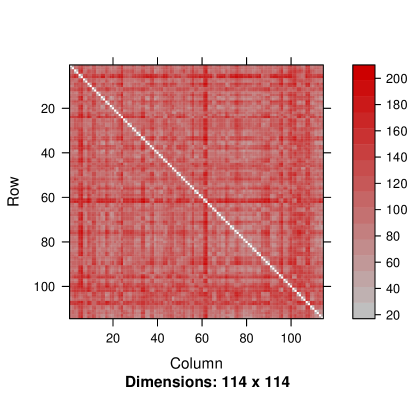
(a)

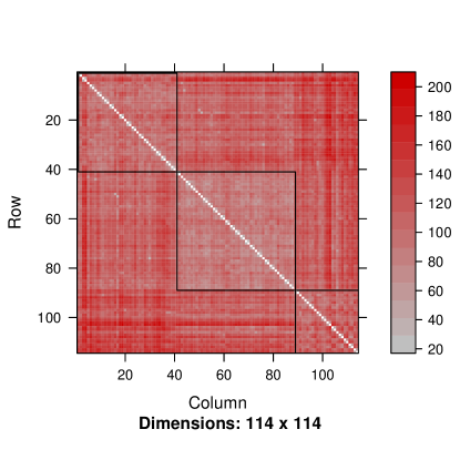
(b)

Figure 3: (a) Omnibus dissimilarity matrix $\mathbf{D}$ across 114 graphs. (b) Results of hierarchical clustering of this dissimilarity matrix.

Using classical multidimensional scaling (Cox and Cox, 2000), we embed this dissimilarity matrix into $2$-dimensional Euclidean space. This yields a collection of 114 points in $\mathbb{R}^{2}$, each one of which represents one graph. We then cluster this collection of points using Gaussian mixture modeling, in which we select $c=3$ clusters according to the Bayesian Information Criterion (BIC). The three resulting clusters are depicted in Fig. 4(b). We remark that out of 57 subjects, only 10 subject scans are divided across clusters, suggesting that the clusters capture meaningful similarity across graphs.

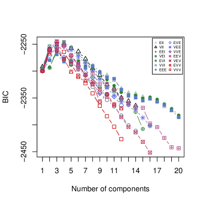
(a)

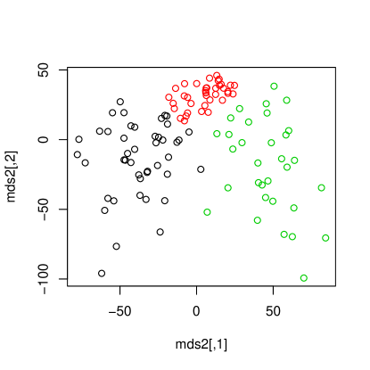
(b)

Figure 4: (a) Clustering using Gaussian mixture modeling and selection of $c=3$ clusters as applied to the $2$-dimensional CMDS embedding of $\mathbf{D}$. (b) Visualization of the embeddings and their resulting clusters. Each point represents a single graph from the BNU1 data set.

If it were truly the case that all of these graphs had the same latent positions, our main central limit theorem would ensure that for large graph sizes these embedded points would be asymptotically normal. Thus, if we consider these three clusters as identifying three distinct types of graphs, we can now compare embedded latent positions of individual vertices across graphs to determine which vertices play the most similar or different roles in their respective graphs. The (theoretical) asymptotic normality leads us to consider a multivariate analysis of variance (MANOVA). For each vertex, we consider the embedded points corresponding to that vertex that arise from the graphs in Cluster 1, Cluster 2, and Cluster 3, respectively. Because we have multiple embedded points for each vertex and these embedded points are asymptotically normal, MANOVA is, as an exploratory tool, principled. MANOVA produces $p$-value for each vertex, associated to the test of equality of the true mean vectors for the normal distributions governing the embedded points in each of the $3$ classes Since there are 172 vertices, we obtain 172 corresponding $p$-values, and we correct for multiple comparisons using the Bonferroni correction. The $p$-values are ordered by significance in Fig. 5.

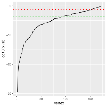
Figure 5: MANOVA $p$-values, with vertices sorted by significance and adjusted for multiple comparisons. The dotted lines indicate the $p=0.05$ threshold (green) and the threshold after Bonferroni correction.

We focus on one of the two most significant vertices, Vertex 98. Recall that by nature of the omnibus embedding, we have multiple points embedded in $\mathbb{R}^{\hat{d}}$, each of which correspond to the $98$-th vertex in one of the 114 graphs. Partitioning these $114$ points according to the clusters associated to their respective graphs, we can perform nonparametric tests of difference across these collections of points to further illuminate how this vertex differs in its behavior across the three graph clusters. Fig. 6 illustrates how strikingly different are the first two principal dimensions of the embedded points for this vertex across the three different clusters. For contrast, we examine one of the least significant vertices, Vertex 124, and reproduce the analogous plots to those in Fig.6 for its first principal dimension. The results are displayed in Fig. 7.

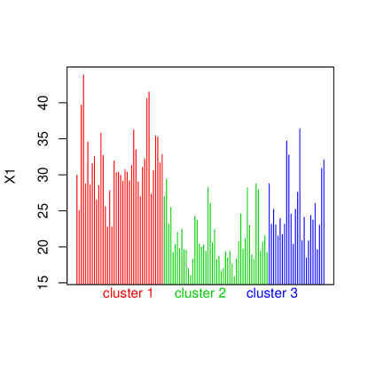
(a)

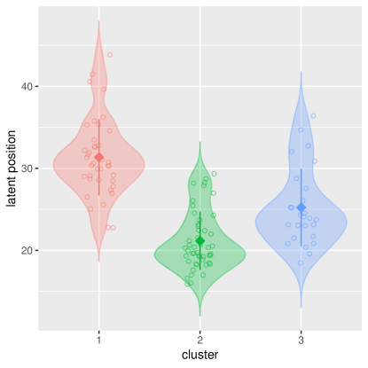
(b)

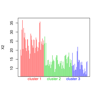
(c)

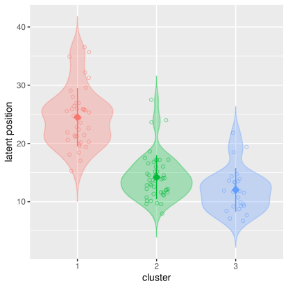
(d)

Figure 6: (a) For the most significant vertex (Vertex 98), a histogram of the first principal dimension of embedded latent position, grouped by cluster. (b) For this same vertex, estimated mean and confidence intervals for the first dimension of the embedded position, again grouped by cluster. (c) and (d) show the analogous plots for the second principal dimension. Observe that the first principal dimension distinguishes between the first and second cluster, and the second principal dimension between the first and the third cluster.

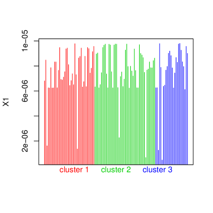
(a)

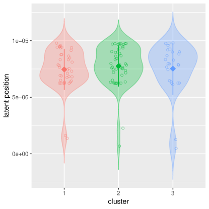
(b)

Figure 7: (a) For the least significant vertex, a histogram of the first dimension of estimated latent positions, grouped by cluster. (b) For this same vertex, estimated means and confidence intervals for the first dimension of the estimated latent position, again grouped by cluster.

The contrast between Figs. 6 and 7 is striking. Because the omnibus embedding gives us multiple points for each vertex, we are able to isolate vertices that are responsible for between-graph differences and then interface with neuroscientists to discern what physical distinctions might be present at this vertex or brain location across the clusters of graphs.

We recognize, of course, some immediate concerns with our procedure. First, the fact that our clusters are determined post-hoc implies that the embedded vectors are not independent samples from different populations. Second, the asymptotic normality of the embedded positions is a large-sample result, and applies to an arbitrary but finitely fixed collection of rows. Despite these limitations, we stress that our theoretical results supply a principled foundation on which to build a more refined analysis, and to date this is among the only approaches for the identification and comparison of individual vertices and their role in driving differences between (populations of) graphs.

2.2 Identifying brain regions associated with schizophrenia

We next consider the COBRE data set (Aine et al., 2017), a collection of scans of both schizophrenic and healthy patients. Each scan yields a graph on $n=264$ vertices, corresponding to 264 brain regions of interest (Power et al., 2011), with edge weights given by correlations between BOLD signals measured in those regions. The data set contains scans for $54$ schizophrenic patients and $69$ healthy controls, for a total of $m=123$ brain graphs.

We follow the general framework of our BNU1 analysis above. Under the null hypothesis that all $m$ graphs share the same underlying latent positions, the omnibus embedding yields for each vertex a collection of $m$ points in $\mathbb{R}^{d}$ that are normally distributed about the true latent position of that vertex. By applying an omnibus embedding to the $m=123$ subjects in the COBRE dataset, we can therefore test, for each vertex $i\in[264]$, whether or not the healthy and schizophrenic populations display a difference in that vertex, by comparing the latent positions of vertex $i$ associated with the schizophrenic patients against those associated with the healthy patients. That is, let $m_{s}=54$ denote the number of schizophrenic patients and $m_{h}=69$ denote the number of healthy controls, with respective embeddings given by

$$\{X^{(j)}_{i}:j=1,2,\dots,m_{s}\},\textrm{ and }\{Y^{(j)}_{i}:j=1,2,\dots,m_{h}\}$$

We can test whether the samples

$$\{X^{(1)}_{i},X^{(2)}_{i},\dots,X^{(m_{h})}\}\subseteq\mathbb{R}^{d}\textrm{ and }\{Y^{(1)}_{i},Y^{(2)}_{i},\dots,Y^{(m_{s})}\}\subseteq\mathbb{R}^{d}$$

appear to come from the same distribution. By Theorem 1, if all $m$ subjects’ graphs are drawn from the same underlying RDPG, then it is natural to test the hypothesis that both the $X_{i}^{(}j)$ and then $Y_{i}^{(}j),1\leq j\leq m_{k}$ are drawn from the same normal distribution. We use Hotelling’s $t^{2}$ test (Hotelling, 1931; Anderson, 2003) (and we remark that experiments applying a permutation test for this same purpose yield broadly similar results). We note that while in the BNU1 data example in Section 2.1, we required a clustering to discover collections of similarly-behaving networks, the COBRE data set already has two populations of interest in the form of the healthy and schizophrenic patients.

We begin by building the omnibus matrix of $m=123$ brain graphs, each on $n=264$ vertices. In contrast to the BNU1 data presented above, here we work with the weighted graph obtained from scans, rather than binarizing them. We apply a three-dimensional omnibus embedding to these $m$ graphs, yielding $123$ points in $\mathbb{R}^{3}$ for each of the $n=264$ brain regions for a total of $32472$ points. For each vertex $i\in\{1,2,\dots,264\}$, there are $m=123$ points in $\mathbb{R}^{3}$ each corresponding to vertex $i$ in one of the brain graphs. $54$ of these $123$ points correspond to the estimated latent position of the $i$-th vertex in the schizophrenic patients, while the remaining $69$ points correspond to the estimated latent position of the $i$-the vertex in the healthy patients. For each vertex $i$, we apply Hotelling’s $t^{2}$ test to assess whether or not the healthy and schizophrenic estimated latent positions appear to come from different populations. Thus, for each of the $264$ regions of interest, we obtain a $p$-value that captures the extent to which the estimated latent positions of the healthy and schizophrenic patients appear to differ in their distributions.

Figure 8 summarizes the result of the procedure just described. Using the Power parcellation (Power et al., 2011), we group the 264 brain regions into larger parcels, which capture what are believed by neuroscientists to correspond to functional subnetworks of the brain. For example, a parcel called the default mode network is associated with wakeful, undirected thought (i.e., mind wandering), and is implicated in schizophrenia (Whitfield-Gabrieli et al., 2009; Fox et al., 2015). We collect, for each of the 14 Power parcels, the $p$-values associated with all of the brain regions (i.e., vertices) in that parcel, and display in Figure 8 a histogram of those $p$-values. Under this setup, parcels in which the populations are largely the same will have histograms that appear more or less flat, while parcels in which schizophrenic patients display different behavior from their healthy counterparts will result in left-skewed histograms. Observing Figure 8, we see strong visual evidence that the default mode, the sensory/somatomotor hand and the uncertain parcels are affected by schizophrenia.

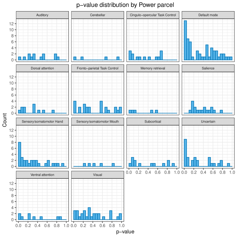
Figure 8: Histograms of the distribution of $p$-values within each parcel. Each histogram corresponds to one of the fourteen parcels in the Power parcellation (Power et al., 2011), and shows the distribution of the $p$-values obtained from applying the Hotelling $t^{2}$ test to the omnibus embeddings of the brain regions in that parcel. We see that certain parcels (most notably the default mode, sensory/somatomotor hand, and uncertain parcels) clearly display non-uniform $p$-value distributions, suggesting that these parcels differ in schizophrenic patients compared to their healthy counterparts.

Here again we see the utility of the omnibus embedding. Thanks to the alignment of the embeddings across all $123$ graphs in the sample, we obtain, after comparatively little processing, a concise summary of which vertices differ in their behavior across the two populations of interest. Further, this information can be summarized into an simple display of information—in this case, summarizing which Power parcels are likely involved in schizophrenia—that is interpretable by neuroscientists and other domain specialists.

3 Background, notation, and definitions

We now turn toward a more thorough exploration of the theoretical results alluded to above. We begin by establishing notation and a few definitions that will prove useful in the sequel.

3.1 Notation and Definitions

For a positive integer $n$, we let $[n]=\{1,2,\dots,n\}$, and denote the identity, zero and all-ones matrices by, respectively, $\mathbf{I}$, $\mathbf{0}$ and $\mathbf{J}$. For an $n\times n$ matrix $\mathbf{H}$, we let $\lambda_{i}(\mathbf{H})$ denote the $i$-th largest eigenvalue of $\mathbf{H}$ and we let $\sigma_{i}(\mathbf{H})$ denote the $i$-th singular value of $\mathbf{H}$. We use $\otimes$ to denote the Kronecker product. For a vector $\mathbf{v}$, we let $\|\mathbf{v}\|$ denote the Euclidean norm of $\mathbf{v}$. For a matrix $\mathbf{H}\in\mathbb{R}^{n_{1}\times n_{2}}$, we denote by $\mathbf{H}_{\cdot j}$ the column vector formed by the $j$-th column of $\mathbf{H}$, and let $\mathbf{H}_{i\cdot}$ denote the row vector formed by the $i$-th row of $\mathbf{H}$. For ease of notation, we let $\mathbf{H}_{i}\in\mathbb{R}^{n_{2}}$ denote the column vector formed by transposing the $i$-th row of $\mathbf{H}$. That is, $\mathbf{H}_{i}=(\mathbf{H}_{i\cdot})^{T}$. We let $\|\mathbf{H}\|$ denote the spectral norm of $\mathbf{H}$, $\|\mathbf{H}\|_{F}$ denote the Frobenius norm of $\mathbf{H}$ and $\|\mathbf{H}\|_{2\rightarrow\infty}$ denote the maximum of the Euclidean norms of the rows of $\mathbf{H}$, i.e., $\|\mathbf{H}\|_{2\rightarrow\infty}=\max_{i}\|\mathbf{H}_{i}\|$. Where there is no danger of confusion, we will often refer to a graph $G$ and its adjacency matrix $\mathbf{A}$ interchangeably. Throughout, we will use $C>0$ to denote a constant, not depending on $n$, whose value may vary from one line to another. For an event $E$, we denote its complement by $E^{c}$. Given a sequence of events $\{E_{n}\}$, we say that $E_{n}$ occurs with high probability, and write $E_{n}\text{ w.h.p. }$, if $\Pr[E_{n}^{c}]\leq Cn^{-2}$ for $n$ sufficiently large. We note that $E_{n}$ w.h.p. implies, by the Borel-Cantelli Lemma, that with probability $1$ there exists an $n_{0}$ such that $E_{n}$ holds for all $n\geq n_{0}$.

Our focus here is on $d$-dimensional random dot product graphs, for which the edge connection probabilities arise as inner products between vectors, called latent positions, that are associated to the vertices. Therefore, we define an an inner product distribution as a probability distribution over a suitable subset of $\mathbb{R}^{d}$, as follows:

Definition 1.

($d$-dimensional Inner Product Distribution) Let $F$ be a probability distribution on $\mathbb{R}^{d}$. We say that $F$ is a $d$-dimensional inner product distribution on $\mathbb{R}^{d}$ if for all $\mathbf{x},\mathbf{y}\in\operatorname{supp}F$, we have $\mathbf{x}^{T}\mathbf{y}\in[0,1]$.

Definition 2.

(Random Dot Product Graph) Let $F$ be a $d$-dimensional inner product distribution with $\mathbf{X}_{1},\mathbf{X}_{2},\dots,\mathbf{X}_{n}\stackrel{{\scriptstyle\text{i.i.d.}}}{{\sim}}F$, collected in the rows of the matrix $\mathbf{X}=[\mathbf{X}_{1},\mathbf{X}_{2},\dots,\mathbf{X}_{n}]^{T}\in\mathbb{R}^{n\times d}$. Suppose $\mathbf{A}$ is a random adjacency matrix given by

$$\Pr[\mathbf{A}|\mathbf{X}]=\prod_{i<j}(\mathbf{X}_{i}^{T}\mathbf{X}_{j})^{\mathbf{A}_{ij}}(1-\mathbf{X}_{i}^{T}\mathbf{X}_{j})^{1-\mathbf{A}_{ij}}$$ (3)

We then write $(\mathbf{A},\mathbf{X})\sim\operatorname{RDPG}(F,n)$ and say that $\mathbf{A}$ is the adjacency matrix of a random dot product graph with latent positions given by the rows of $\mathbf{X}$.

We note that we restrict our attention here to hollow, undirected graphs.

Given $\mathbf{X}$, the probability $p_{ij}$ of observing an edge between vertex $i$ and vertex $j$ is simply $\mathbf{X}_{i}^{T}\mathbf{X}_{j}$, the dot product of the associated latent positions $\mathbf{X}_{i}$ and $\mathbf{X}_{j}$. We define the matrix of such probabilities by $\mathbf{P}=[p_{ij}]=\mathbf{X}\mathbf{X}^{T}$, and write $\mathbf{A}\sim\operatorname{Bernoulli}(\mathbf{P})$ to denote that the existence of an edge between any two vertices $1\leq i<j\leq n$ is a Bernoulli random variable with probability $p_{ij}$, with these edges independent. That is, if $\mathbf{P}=\mathbf{X}\mathbf{X}^{T}$, then $\mathbf{A}\sim\operatorname{Bernoulli}(\mathbf{P})$ implies that conditioned on $\mathbf{X}$, $\mathbf{A}$ is distributed as in Eq. (3).

Remark 1.

Note that if $\mathbf{X}\in\mathbb{R}^{n\times d}$ is a matrix of latent positions and $\mathbf{W}\in\mathbb{R}^{d\times d}$ is orthogonal, $\mathbf{X}$ and $\mathbf{X}\mathbf{W}$ give rise to the same distribution over graphs in Equation (3). Thus, the RDPG model has a nonidentifiability up to orthogonal transformation.

The focus of this paper is on multi-graph inference. As such, we consider a collection of $m$ random dot product graphs, all with the same latent positions, which motivates the following definition:

Definition 3.

(Joint Random Dot Product Graph) Let $F$ be a $d$-dimensional inner product distribution on $\mathbb{R}^{d}$. We say that random graphs $\mathbf{A}^{(1)},\mathbf{A}^{(2)},\dots,\mathbf{A}^{(m)}$ are distributed as a joint random dot product graph (JRDPG) and write $(\mathbf{A}^{(1)},\mathbf{A}^{(2)},\dots,\mathbf{A}^{(m)},\mathbf{X})\sim\operatorname{JRDPG}(F,n,m)$ if $\mathbf{X}=[\mathbf{X}_{1},\mathbf{X}_{2},\dots,\mathbf{X}_{n}]^{T}\in\mathbb{R}^{n\times d}$ has its (transposed) rows distributed i.i.d. as $\mathbf{X}_{i}\sim F$, and we have marginal distributions $(\mathbf{A}^{(k)},\mathbf{X})\sim\operatorname{RDPG}(F,n)$ for each $k=1,2,\dots,m$. That is, the $\mathbf{A}^{(k)}$ are conditionally independent given $\mathbf{X}$, with edges independently distributed as $\mathbf{A}^{(k)}_{i,j}\sim\operatorname{Bernoulli}((\mathbf{X}\mathbf{X}^{T})_{ij})$ for all $1\leq i<j\leq n$ and all $k\in[m]$.

Throughout, we let $\delta>0$ denote the eigengap of

$$\mathbf{\Delta}=\mathbb{E}\mathbf{X}_{1}\mathbf{X}_{1}^{T}\in\mathbb{R}^{d\times d},$$ (4)

the second moment matrix of $\mathbf{X}_{1}\sim F$. That is, $\delta=\lambda_{d}(\mathbf{\Delta})>0=\lambda_{d+1}(\mathbf{\Delta})$. We note that $\mathbf{\Delta}$ can be chosen diagonal without loss of generality after a suitable change of basis (Athreya et al., 2016). We assume further that $\mathbf{\Delta}$ is such that its diagonal entries are in nonincreasing order, so that $\mathbf{\Delta}_{1,1}\geq\mathbf{\Delta}_{2,2}\geq\dots\geq\mathbf{\Delta}_{d,d}=\delta.$ We assume that the matrix $\mathbf{\Delta}$ is constant in $n$, so that $d$ and $\delta$ are constants, while the number of graphs $m$ is allowed to grow with $n$. We leave for future work the exploration of the case where the model parameters are allowed to vary with the number of vertices $n$.

Since we rely on spectral decompositions, we begin with a straightforward one: the spectral decomposition of the positive semidefinite matrix $\mathbf{P}=\mathbf{X}\mathbf{X}^{T}$.

Definition 4.

(Spectral Decomposition of $\mathbf{P}$) Since $\mathbf{P}$ is symmetric and positive semidefinite, let $\mathbf{P}=\mathbf{U}_{\mathbf{P}}\mathbf{S}_{\mathbf{P}}\mathbf{U}_{\mathbf{P}}^{T}$ denote its spectral decomposition, with $\mathbf{U}_{\mathbf{P}}\in\mathbb{R}^{n\times d}$ having orthonormal columns and $\mathbf{S}_{\mathbf{P}}\in\mathbb{R}^{d\times d}$ diagonal with nonincreasing entries $(\mathbf{S}_{\mathbf{P}})_{1,1}\geq(\mathbf{S}_{\mathbf{P}})_{2,2}\geq\cdots\geq(\mathbf{S}_{\mathbf{P}})_{d,d}>0$.

We note that while $\mathbf{P}=\mathbf{X}\mathbf{X}^{T}$ is not observed, existing spectral norm bounds (e.g., Oliveira, 2009; Lu and Peng, 2013) establish that if $\mathbf{A}\sim\operatorname{Bernoulli}(\mathbf{P})$, the spectral norm of $\mathbf{A}-\mathbf{P}$ is comparatively small. As a result, we regard $\mathbf{A}$ as a noisy version of $\mathbf{P}$, and we begin our inference procedures with a spectral decomposition of $\mathbf{A}$.

Definition 5.

(Adjacency Spectral Embedding; Sussman et al., 2012) Let $\mathbf{A}\in\mathbb{R}^{n\times n}$ be the adjacency matrix of an undirected $d$-dimensional random dot product graph. The $d$-dimensional adjacency spectral embedding (ASE) of $\mathbf{A}$ is a spectral decomposition of $\mathbf{A}$ based on its top $d$ eigenvalues, obtained by $\operatorname{ASE}(\mathbf{A},d)=\mathbf{U}_{\mathbf{A}}\mathbf{S}_{\mathbf{A}}^{1/2}$, where $\mathbf{S}_{\mathbf{A}}\in\mathbb{R}^{d\times d}$ is a diagonal matrix whose entries are the top eigenvalues of $\mathbf{A}$ (in nonincreasing order) and $\mathbf{U}_{\mathbf{A}}\in\mathbb{R}^{n\times d}$ is the matrix whose columns are the orthonormal eigenvectors corresponding to the eigenvalues in $\mathbf{S}_{\mathbf{A}}$.

Remark 2.

We observe that without any additional assumptions, the top $d$ eigenvalues of $\mathbf{A}$ are not guaranteed to be nonnegative. However, under our eigengap assumptions on $\mathbf{\Delta}$, the i.i.d.-ness of the latent positions ensures that for large $n$, the eigenvalues of $\mathbf{A}$ will be nonnegative with high probability (see Observation 2 in the Supplementary Material).

Given a set of $m$ adjacency matrices distributed as

$$(\mathbf{A}^{(1)},\mathbf{A}^{(2)},\dots,\mathbf{A}^{(m)},\mathbf{X})\sim\operatorname{JRDPG}(F,n,m)$$

for distribution $F$ on $\mathbb{R}^{d}$, a natural inference task is to recover the $n$ latent positions $\mathbf{X}_{1},\mathbf{X}_{2},\dots,\mathbf{X}_{n}\in\mathbb{R}^{d}$ shared by the vertices of the $m$ graphs. To estimate the underlying latent positions from these $m$ graphs, Tang et al. (2016) provides justification for the estimate $\bar{\mathbf{X}}=\operatorname{ASE}(\bar{\mathbf{A}},d)$, where $\bar{\mathbf{A}}$ is the sample mean of the adjacency matrices $\mathbf{A}^{(1)},\mathbf{A}^{(2)},\dots,\mathbf{A}^{(m)}$. However, $\bar{\mathbf{X}}$ is ill-suited to any task that requires comparing latent positions across the $m$ graphs, since the $\bar{\mathbf{X}}$ estimate collapses the $m$ graphs into a single set of $n$ latent positions. This motivates the omnibus embedding, which still yields a single spectral decomposition, but with a separate $d$-dimensional representation for each of the $m$ graphs. This makes the omnibus embedding useful for simultaneous inference across all $m$ observed graphs.

Definition 6.

(Omnibus embedding) Let $\mathbf{A}^{(1)},\mathbf{A}^{(2)},\dots,\mathbf{A}^{(m)}\in\mathbb{R}^{n\times n}$ be (possibly weighted) adjacency matrices of a collection of $m$ undirected graphs. We define the $mn$-by-$mn$ omnibus matrix of $\mathbf{A}^{(1)},\mathbf{A}^{(2)},\dots,\mathbf{A}^{(m)}$ by

$$\mathbf{M}=\begin{bmatrix}\mathbf{A}^{(1)}&\frac{1}{2}(\mathbf{A}^{(1)}+\mathbf{A}^{(2)})&\dots&\frac{1}{2}(\mathbf{A}^{(1)}+\mathbf{A}^{(m)})\\ \frac{1}{2}(\mathbf{A}^{(2)}+\mathbf{A}^{(1)})&\mathbf{A}^{(2)}&\dots&\frac{1}{2}(\mathbf{A}^{(2)}+\mathbf{A}^{(m)})\\ \vdots&\vdots&\ddots&\vdots\\ \frac{1}{2}(\mathbf{A}^{(m)}+\mathbf{A}^{(1)})&\frac{1}{2}(\mathbf{A}^{(m)}+\mathbf{A}^{(2)})&\dots&\mathbf{A}^{(m)}\end{bmatrix},$$ (5)

and the $d$-dimensional omnibus embedding of $\mathbf{A}^{(1)},\mathbf{A}^{(2)},\dots,\mathbf{A}^{(m)}$ is the adjacency spectral embedding of $\mathbf{M}$:

$$\operatorname{OMNI}(\mathbf{A}^{(1)},\mathbf{A}^{(2)},\dots,\mathbf{A}^{(m)},d)=\operatorname{ASE}(\mathbf{M},d).$$

If $(\mathbf{A}^{(1)},\mathbf{A}^{(2)},\dots,\mathbf{A}^{(m)},\mathbf{X})\sim\operatorname{JRDPG}(F,n,m)$, then the omnibus embedding provides a natural approach to estimating $\mathbf{X}$ without collapsing the $m$ graphs into a single representation as with $\bar{\mathbf{X}}=\operatorname{ASE}(\bar{\mathbf{A}},d)$. Under the JRDPG, the omnibus matrix has expected value

$$\mathbb{E}\mathbf{M}=\tilde{\mathbf{P}}=\mathbf{J}_{m}\otimes\mathbf{P}=\mathbf{U}_{\tilde{\mathbf{P}}}\mathbf{S}_{\tilde{\mathbf{P}}}\mathbf{U}_{\tilde{\mathbf{P}}}^{T}$$

for $\mathbf{U}_{\tilde{\mathbf{P}}}\in\mathbb{R}^{mn\times d}$ having $d$ orthonormal columns and $\mathbf{S}_{\tilde{\mathbf{P}}}\in\mathbb{R}^{d\times d}$ diagonal. Since $\mathbf{M}$ is a reasonable estimate for $\tilde{\mathbf{P}}=\mathbb{E}\mathbf{M}$ (see, for example, Oliveira, 2009), the matrix $\hat{\mathbf{Z}}=\operatorname{OMNI}(\mathbf{A}^{(1)},\mathbf{A}^{(2)},\dots,\mathbf{A}^{(m)},d)$ is a natural estimate of the $mn$ latent positions collected in the matrix $\mathbf{Z}=[\mathbf{X}^{T}\mathbf{X}^{T}\dots\mathbf{X}^{T}]^{T}\in\mathbb{R}^{mn\times d}$. Here again, as in Remark 1, $\hat{\mathbf{Z}}$ only recovers the true latent positions $\mathbf{Z}$ up to an orthogonal rotation. The matrix

$$\mathbf{Z}^{*}=\begin{bmatrix}\mathbf{X}^{*}\\ \mathbf{X}^{*}\\ \vdots\\ \mathbf{X}^{*}\end{bmatrix}=\mathbf{U}_{\tilde{\mathbf{P}}}\mathbf{S}_{\tilde{\mathbf{P}}}^{1/2}\in\mathbb{R}^{mn\times d},$$ (6)

provides a reasonable canonical choice of latent positions, so that $\mathbf{Z}=\mathbf{Z}^{*}\mathbf{W}$ for some suitably-chosen orthogonal matrix $\mathbf{W}\in\mathbb{R}^{d\times d}$, and our main theorem shows that we can recover $\mathbf{Z}$ (up to orthogonal rotation) by recovering $\mathbf{Z}^{*}$.

4 Main Results

In this section, we give theoretical results on the consistency and asymptotic distribution of the estimated latent positions based on the omnibus matrix $\mathbf{M}$. In the next section, we demonstrate from simulations that the omnibus embedding can be successfully leveraged for subsequent inference, specifically two-sample testing.

Lemma 1 shows that the omnibus embedding provides uniformly consistent estimates of the true latent positions, up to an orthogonal transformation, roughly analogous to Lemma 5 in Lyzinski et al. (2014). Lemma 1 shows consistency of the omnibus embedding under the $2\rightarrow\infty$ norm, implying that all $mn$ of the estimated latent positions are near their corresponding true positions. We recall that the orthogonal transformation $\tilde{\mathbf{W}}$ in the statement of the lemma is necessary since, as discussed in Remark 1, $\mathbf{P}=\mathbf{X}\mathbf{X}^{T}=(\mathbf{X}\mathbf{W})(\mathbf{X}\mathbf{W})^{T}$ for any orthogonal $\mathbf{W}\in\mathbb{R}^{d\times d}$.

Lemma 1.

With $\tilde{\mathbf{P}}$, $\mathbf{M}$, $\mathbf{U}_{\mathbf{M}}$, and $\mathbf{U}_{\tilde{\mathbf{P}}}$ defined as above, there exists an orthogonal matrix $\tilde{\mathbf{W}}\in\mathbb{R}^{d\times d}$ such that with high probability,

$$\|\mathbf{U}_{\mathbf{M}}\mathbf{S}_{\mathbf{M}}^{1/2}-\mathbf{U}_{\tilde{\mathbf{P}}}\mathbf{S}_{\tilde{\mathbf{P}}}^{1/2}\tilde{\mathbf{W}}\|_{2\rightarrow\infty}\leq\frac{Cm^{1/2}\log mn}{\sqrt{n}}.$$ (7)

Proof.

This result is proved in the supplemental material. ∎

As noted earlier, our central limit theorem for the omnibus embedding is analogous to a similar result proved in Athreya et al. (2016), but with the crucial difference that we no longer require that the second moment matrix have distinct eigenvalues. As in Athreya et al. (2016), our proof here depends on writing the difference between a row of the omnibus embedding and its corresponding latent position as a pair of summands: the first, to which a classical Central Limit Theorem can be applied, and the second, essentially a combination of residual terms, which converges to zero. The weakening of the assumption of distinct eigenvalues necessitates significant changes in how to bound the residual terms. In fact, Athreya et al. (2016) adapts a result of Bickel and Sarkar (2015)—the latter of which depends on the assumption of distinct eigenvalues—to control these terms. Here, we resort to somewhat different methodology: we prove instead that analogous bounds to those in Lyzinski et al. (2017); Tang and Priebe (2018) hold for the estimated latent positions based on the omnibus matrix $\mathbf{M}$, and this enables us to establish that here, too, the rows of the omnibus embedding are also approximately normally distributed. Further, en route to this limiting result, we compute the explicit variance of the omnibus matrix, and show that as $m$, the number of graphs embedded, increases, this contributes to a reduction in the variance of the estimated latent positions.

Theorem 1.

Let $(\mathbf{A}^{(1)},\mathbf{A}^{(2)},\dots,\mathbf{A}^{(m)},\mathbf{X})\sim\operatorname{JRDPG}(F,n,m)$ for some $d$-dimensional inner product distribution $F$ and let $\mathbf{M}$ denote the omnibus matrix as in (5). Let $\mathbf{Z}=\mathbf{Z}^{*}\mathbf{W}$ with $\mathbf{Z}^{*}$ as defined in Equation (6), with estimate $\hat{\mathbf{Z}}=\operatorname{OMNI}(\mathbf{A}^{(1)},\mathbf{A}^{(2)},\dots,\mathbf{A}^{(m)},d)$. Let $h=m(s-1)+i$ for $i\in[n],s\in[m]$, so that $\hat{\mathbf{Z}}_{h}$ denotes the estimated latent position of the $i$-th vertex in the $s$-th graph $\mathbf{A}^{(s)}$. That is, $\hat{\mathbf{Z}}_{h}$ is the column vector formed by transposing the $h$-th row of the matrix $\hat{\mathbf{Z}}=\mathbf{U}_{\mathbf{M}}\mathbf{S}_{\mathbf{M}}^{1/2}=\operatorname{OMNI}(\mathbf{A}^{(1)},\mathbf{A}^{(2)},\dots,\mathbf{A}^{(m)},d)$. Let $\Phi(\mathbf{x},\mathbf{\Sigma})$ denote the cdf of a (multivariate) Gaussian with mean zero and covariance matrix $\mathbf{\Sigma}$, evaluated at $\mathbf{x}\in\mathbb{R}^{d}$. There exists a sequence of orthogonal $d$-by-$d$ matrices $(\tilde{\mathbf{W}}_{n})_{n=1}^{\infty}$ such that for all $\mathbf{x}\in\mathbb{R}^{d}$,

$$\lim_{n\rightarrow\infty}\Pr\left[n^{1/2}\left(\hat{\mathbf{Z}}\tilde{\mathbf{W}}_{n}-\mathbf{Z}\right)_{h}\leq\mathbf{x}\right]=\int_{\operatorname{supp}F}\Phi\left(\mathbf{x},\mathbf{\Sigma}(\mathbf{y})\right)dF(\mathbf{y}),$$

where $\mathbf{\Sigma}(\mathbf{y})=(m+3)\mathbf{\Delta}^{-1}\tilde{\mathbf{\Sigma}}(\mathbf{y})\mathbf{\Delta}^{-1}/(4m),$ $\mathbf{\Delta}$ is as defined in (4) and

$$\tilde{\mathbf{\Sigma}}(\mathbf{y})=\mathbb{E}\left[(\mathbf{y}^{T}\mathbf{X}_{1}-(\mathbf{y}^{T}\mathbf{X}_{1})^{2})\mathbf{X}_{1}\mathbf{X}_{1}^{T}\right].$$

Proof.

This result is proved in the supplemental material. ∎

5 Experimental results

In this section, we present experiments on synthetic data exploring the efficacy of the omnibus embedding described above. We consider both estimation of latent positions and two-sample graph testing.

5.1 Recovery of Latent Positions

Perhaps the most ubiquitous estimation problem for RDPG data is that of estimating the latent positions (i.e., the rows of the matrix $\mathbf{X}$); consequently, we begin by exploring how well the omnibus embedding recovers the latent positions of a given random dot product graph. If one wishes merely to estimate the latent positions $\mathbf{X}$ of a set of $m$ graphs $(\mathbf{A}^{(1)},\mathbf{A}^{(2)},\dots,\mathbf{A}^{(m)},\mathbf{X})\sim\operatorname{JRDPG}(F,n,m)$, the estimate $\bar{\mathbf{X}}=\operatorname{ASE}(\sum_{i=1}^{m}\mathbf{A}^{(i)}/m,d)$, the embedding of the sample mean of the adjacency matrices performs well asymptotically (Tang et al., 2016). Indeed, all else equal, the embedding $\bar{\mathbf{X}}$ is preferable to the omnibus embedding if only because it requires an eigendecomposition of an $n$-by-$n$ matrix rather than the much larger $mn$-by-$mn$ omnibus matrix.

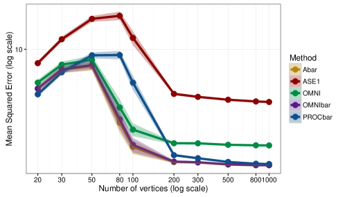
Figure 9: Mean squared error (MSE) in recovery of latent positions (up to rotation) in a 2-graph joint RDPG model as a function of the number of vertices. The figure shows the performance of ASE applied to a single graph (red), ASE embedding of the mean graph (gold), the Procrustes-based pairwise embedding (blue), the omnibus embedding (green) and the mean omnibus embedding (purple). Each point is the mean of 50 trials, with error bars indicating two times the standard error. We see that the mean omnibus embedding (OMNIbar) achieves performance competitive with that of the optimal embedding $\operatorname{ASE}(\bar{\mathbf{A}},d)$, while the Procrustes alignment estimation is notably inferior to the other two-graph techniques for graphs of size between 80 and 200 vertices (and we note that the gap appears to persist at larger graph sizes, though it shrinks).

Of course, the omnibus embedding can still be used to to estimate the latent positions, potentially at the cost of increased variance. Figure 9 compares the mean-squared error of various techniques for estimating the latent positions for a random dot product graph. The figure plots the (empirical) mean squared error in recovering the latent positions of a $3$-dimensional JRDPG as a function of the number of vertices $n$. Each point in the plot is the empirical mean of 50 independent trials. In each trial, the vertex latent positions are drawn i.i.d. from a Dirichlet with parameter $[1,\,1,\,1]^{T}\in\mathbb{R}^{3}$. Having generated a random set of latent positions, we generate two graphs, $\mathbf{A}^{(1)},\mathbf{A}^{(2)}\in\mathbb{R}^{n\times n}$ independently, based on this set of latent positions. Thus, we have $(\mathbf{A}^{(1)},\mathbf{A}^{(2)},\mathbf{X})\sim\operatorname{JRDPG}(F,n,2)$, where $F=\operatorname{Dir}([1,\,1,\,1]^{T})$ is a Dirichlet with parameter $[1,\,1,\,1]^{T}\in\mathbb{R}^{3}$, and $n$ varies. The lines correspond to

1. ASE1 (red): we embed only one of the two observed graphs, and use only the ASE of that graph to estimate the latent positions in $\mathbf{X}$. That is, we consider $\operatorname{ASE}(\mathbf{A}^{(1)})$ as our estimate of $\mathbf{X}$, ignoring entirely the information present in $\mathbf{A}^{(2)}$. This condition serves as a baseline for how much additional information is provided by the second graph $\mathbf{A}^{(2)}$.

2. Abar (gold): we embed the average of the two graphs, $\bar{\mathbf{A}}=(\mathbf{A}^{(1)}+\mathbf{A}^{(2)})/2$ as $\hat{\mathbf{X}}=\operatorname{ASE}(\bar{\mathbf{A}},3)$. As discussed in, for example, Tang et al. (2016), this is the lowest-variance estimate of the latent positions $\mathbf{X}$.

3. OMNI (green): We apply the omnibus embedding to obtain $\hat{\mathbf{Z}}=\operatorname{ASE}(\mathbf{M},3)$, where $\mathbf{M}$ is as in Equation (5). We then use only the first $n$ rows of $\hat{\mathbf{Z}}\in\mathbb{R}^{2n\times d}$ as our estimate of $\mathbf{X}$. Thus, this embedding takes advantage of the information available in both graphs $\mathbf{A}^{(1)}$ and $\mathbf{A}^{(2)}$, but does not use both graphs equally, since the first rows of $\hat{\mathbf{Z}}$ are based primarily on the information contained in $\mathbf{A}^{(1)}$.

4. OMNIbar (purple): We again apply the omnibus embedding to obtain estimated latent positions $\hat{\mathbf{Z}}=\operatorname{ASE}(\mathbf{M},3)$, but this time we use all available information by averaging the first $n$ rows and the second $n$ rows of $\hat{\mathbf{Z}}$.

5. PROCbar (blue): We separately embed the graphs $\mathbf{A}^{(1)}$ and $\mathbf{A}^{(2)}$, obtaining two separate estimates of the latent positions in $\mathbb{R}^{3}$. We then align these two sets of estimated latent positions via Procrustes alignment, and average the aligned embeddings to obtain our final estimate of the latent positions.

First, let us note that ASE applied to a single graph (red) lags all other methods. This is expected, since all other methods assessed in Figure 9 use information from both observed graphs $\mathbf{A}^{(1)}$ and $\mathbf{A}^{(2)}$ rather than only $\mathbf{A}^{(1)}$. We see that all other methods perform essentially equally well on graphs of 50 vertices or fewer. Given the dearth of signal in these smaller graphs, we do not expect any method to recover the latent positions accurately.

Crucially, however, we see that the OMNIbar estimate (purple) performs nearly identically to the Abar estimate (gold), the natural choice among spectral methods for the estimation latent positions (for more on the efficiency of Abar, see Tang et al., 2016). The Procrustes estimate (in blue) provides a two-graph analogue of ASE (red): it combines two ASE estimates via Procrustes alignment, but does not enforce an a priori alignment of the estimated latent positions in the manner of the omnibus embedding does (we discuss this enforced alignment in 6 as well.) As predicted by the results in Lyzinski et al. (2014) and Tang et al. (2017a), the Procrustes estimate is competitive with the Abar (gold) estimate for suitably large graphs. The OMNI estimate (in green) serves, in a sense, as an in-between method, in that it uses information available from both graphs, but in contrast to Procrustes (blue), OMNIbar (purple) and Abar (gold), it does not make complete use of the information available in the second graph. For this reason, it is noteworthy that the OMNI estimate outperforms the Procrustes estimate for graphs of 80-100 vertices. That is, for certain graph sizes, the omnibus estimate appears to more optimally leverage the information in both graphs than the Procrustes estimate does, despite the fact that the information in the second graph has comparatively little influence on the OMNI embedding.

5.2 Two-graph Hypothesis Testing

We now turn to the matter of using the omnibus embedding for testing the semiparametric hypothesis that two observed graphs are drawn from the same underlying latent positions. Suppose we have a set of points $\mathbf{X}_{1},\mathbf{X}_{2},\dots,\mathbf{X}_{n},\mathbf{Y}_{1},\mathbf{Y}_{2},\dots,\mathbf{Y}_{n}\in\mathbb{R}^{d}$. Let the graph $G_{1}$ with adjacency matrix $\mathbf{A}^{(1)}$ have edges distributed independently as $\mathbf{A}^{(1)}_{ij}\sim\operatorname{Bernoulli}(\mathbf{X}_{i}^{T}\mathbf{X}_{j})$. Similarly, let $G_{2}$ have adjacency matrix $\mathbf{A}^{(2)}$ with edges distributed independently as $\mathbf{A}^{(2)}_{ij}\sim\operatorname{Bernoulli}(\mathbf{Y}_{i}^{T}\mathbf{Y}_{j})$. As discussed previously, while $\bar{\mathbf{A}}=(\mathbf{A}^{(1)}+\mathbf{A}^{(2)})/2$ may be optimal for estimation of latent positions, it is not clear how to use the embedding $\operatorname{ASE}(\bar{\mathbf{A}},d)$ to test the following hypothesis:

$$H_{0}:\mathbf{X}_{i}=\mathbf{Y}_{i}\enspace\forall i\,\in[n].$$ (8)

On the other hand, the omnibus embedding provides a natural test of the null hypothesis (8) by comparing the first $n$ and last $n$ embeddings of the omnibus matrix

$$\mathbf{M}=\begin{bmatrix}\mathbf{A}^{(1)}&(\mathbf{A}^{(1)}+\mathbf{A}^{(2)})/2\\ (\mathbf{A}^{(1)}+\mathbf{A}^{(2)})/2&\mathbf{A}^{(2)}\end{bmatrix}.$$

Intuitively, when $H_{0}$ holds, the distributional result in Theorem 1 holds, and the $i$-th and $(n+i)$-th rows of $\operatorname{OMNI}(\mathbf{A}^{(1)},\mathbf{A}^{(2)},d)$ are equidistributed (though they are not independent). On the other hand, when $H_{0}$ fails to hold, there exists at least one $i\in[n]$ for which the $i$-th and $(n+i)$-th rows of $\mathbf{M}$ are not identically distributed, and thus the corresponding embeddings are also distributionally distinct. This suggests a test that compares the first $n$ rows of $\operatorname{OMNI}(\mathbf{A}^{(1)},\mathbf{A}^{(2)},d)$ against the last $n$ rows (see below for details). Here, we empirically explore the power this test against its Procrustes-based alternative from Tang et al. (2017a).

Our setup is as follows. We draw $\mathbf{X}_{1},\mathbf{X}_{2},\dots,\mathbf{X}_{n}\in\mathbb{R}^{3}$ i.i.d. according to a Dirichlet distribution $F$ with parameter $\vec{\mathbf{\alpha}}=[1,1,1]^{T}$. Assembling these $n$ points into a matrix $\mathbf{X}=[\mathbf{X}_{1}\mathbf{X}_{2}\dots\mathbf{X}_{n}]^{T}\in\mathbb{R}^{n\times 3},$ we can generate a graph $G_{1}$ with adjacency matrix $\mathbf{A}^{(1)}$ with entries $\mathbf{A}^{(1)}_{ij}\sim\operatorname{Bernoulli}((\mathbf{X}\mathbf{X}^{T})_{ij})$. Thus, $(\mathbf{A}^{(1)},\mathbf{X})\sim\operatorname{RDPG}(F,n)$. We generate a second graph $G_{2}$ by first drawing random points $\mathbf{Z}_{1},\mathbf{Z}_{2},\dots,\mathbf{Z}_{n}\stackrel{{\scriptstyle\text{i.i.d.}}}{{\sim}}F$. Selecting a set of indices $I\subset[n]$ of size $k<n$ uniformly at random from among all such $\binom{n}{k}$ sets, we let $G_{2}$ have latent positions

$$\mathbf{Y}_{i}=\begin{cases}\mathbf{Z}_{i}&\mbox{ if }i\in I\\ \mathbf{X}_{i}&\mbox{ otherwise. }\end{cases}$$

Assembling these points into a matrix $\mathbf{Y}=[\mathbf{Y}_{1},\mathbf{Y}_{2},\dots,\mathbf{Y}_{n}]^{T}\in\mathbb{R}^{n\times 3},$ we generate graph $G_{2}$ with adjacency matrix $\mathbf{A}^{(2)}$ with edges generated independently according to $\mathbf{A}^{(2)}_{ij}\sim\operatorname{Bernoulli}((\mathbf{Y}\mathbf{Y}^{T})_{ij}).$ The task is then to test the hypothesis

$$H_{0}:\mathbf{X}=\mathbf{Y}.$$ (9)

To test this hypothesis, we consider two different tests, one based on a Procrustes alignment of the adjacency spectral embeddings of $G_{1}$ and $G_{2}$ (Tang et al., 2017a) and the other based on the omnibus embedding. Both approaches are based on estimates of the latent positions of the two graphs. In both cases we use a test statistic of the form $T=\sum_{i=1}^{n}\|\hat{\mathbf{X}}_{i}-\hat{\mathbf{Y}}_{i}\|_{F}^{2},$ and accept or reject based on a Monte Carlo estimate of the critical value of $T$ under the null hypothesis, in which $\mathbf{X}_{i}=\mathbf{Y}_{i}$ for all $i\in[n]$. In each trial, we use $500$ Monte Carlo iterates to estimate the distribution of $T$.

We note that in the experiments presented here, we assume that the latent positions $\mathbf{X}_{1},\mathbf{X}_{2},\dots,\mathbf{X}_{n}$ of graph $G_{1}$ are known for sampling purposes, so that the matrix $\mathbf{P}=\mathbb{E}\mathbf{A}^{(1)}$ is known exactly, rather than estimated from the observed adjacency matrix $\mathbf{A}^{(1)}$. This allows us to sample from the true null distribution. As proved in Lyzinski et al. (2014), the estimated latent positions $\hat{\mathbf{X}}_{1}=\operatorname{ASE}(\mathbf{A}^{(1)})$ and $\hat{\mathbf{X}}_{2}=\operatorname{ASE}(\mathbf{A}^{(2)})$ recover the true latent positions $\mathbf{X}_{1}$ and $\mathbf{X}_{2}$ (up to rotation) to arbitrary accuracy in $(2,\infty)$-norm for suitably large $n$ (Lyzinski et al., 2014). Without using this known matrix $\mathbf{P}$, we would require that our matrices have tens of thousands of vertices before the variance associated with estimating the latent positions would no longer overwhelm the signal present in the few altered latent positions.

Three major factors influence the complexity of testing the null hypothesis in Equation (9): the number of vertices $n$, the number of changed latent positions $k=|I|$, and the distances $\|\mathbf{X}_{i}-\mathbf{Y}_{i}\|_{F}$ between the latent positions. The three plots in Figure 10 illustrate the first two of these three factors. These three plots show the power of two different approaches to testing the null hypothesis (9) for different sized graphs and for different values of $k$, the number of altered latent positions. In all three conditions, both methods improve as the number of vertices increases, as expected, especially since we do not require estimation of the underlying expected matrix $\mathbf{P}$ for Monte Carlo estimation of the null distribution of the test statistic. We see that when only one vertex is changed, neither method has power much above $0.25$. However, in the case of $k=5$ and $k=10$, is it clear that the omnibus-based test achieves higher power than the Procrustes-based test, especially in the range of 30 to 250 vertices.

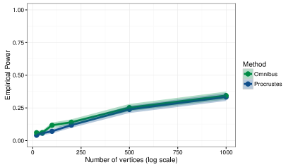
(a)

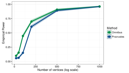
(b)

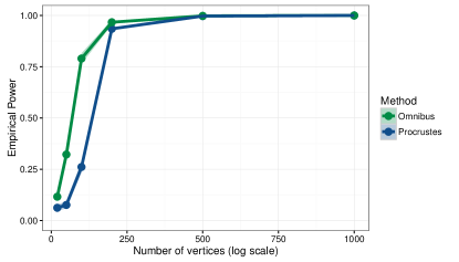
(c)

Figure 10: Power of the ASE-based (blue) and omnibus-based (green) tests to detect when the two graphs being testing differ in (a) one, (b) five, and (c) ten of their latent positions. Each point is the proportion of 1000 trials for which the given technique correctly rejected the null hypothesis, and error bars denote two standard errors of this empirical mean in either direction.

Figure 11 shows the effect of the difference between the latent position matrices under null and alternative. We consider a $3$-dimensional RDPG on $n$ vertices, in which one latent position, $i\in[n]$, is fixed to be equal to $\mathbf{x}_{i}=(0.8,0.1,0.1)^{T}$ and the remaining latent positions are drawn i.i.d. from a Dirichlet with parameter $\vec{\mathbf{\alpha}}=(1,1,1)^{T}$. We collect these latent positions in the rows of the matrix $\mathbf{X}\in\mathbb{R}^{n\times 3}$. To produce the latent positions $\mathbf{Y}\in\mathbb{R}^{n\times 3}$ of the second graph, we use the same latent positions in $\mathbf{X}$, but we alter the $i$-th position to be $\mathbf{Y}_{i}=(1-\lambda)\mathbf{x}_{i}+\lambda(0.1,0.1,0.8)^{T}$ for $\lambda\in[0,1]$ a “drift” parameter, controlling how much the latent position changes between the two graphs. Intuitively, correctly rejecting $H_{0}:\mathbf{X}=\mathbf{Y}$ is easier for larger values of $\lambda$; the greater the gap between latent position matrices under null and alternative, the more easily our test procedure should discriminate between them. Figure 11 shows how the size of the drift parameter influences the power. We see that for $n=30$ vertices (top left), neither the omnibus nor Procrustes test has power appreciably better than approximately $0.05$, largely in agreement with the what we observed in Figure 10. Similarly, when $n=200$ vertices (bottom right), both methods perform approximately equally (though omnibus does appear to consistently outperform Procrustes testing). The case of $n=50$ and $n=100$ vertices (upper right and bottom left, respectively), though, offers a fascinating instance in which the omnibus test consistently outperforms the Procrustes test. Particularly interesting to note is the $n=50$ case (top right), in which we see that performance of the Procrustes test is more or less flat as a function of drift parameter $\lambda$, while the omnibus embedding clearly improves as $\lambda$ increases, with performance climbing well above that of Procrustes for $\lambda>0.8$.

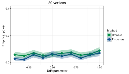
(a)

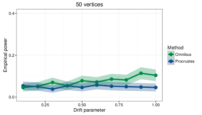
(b)

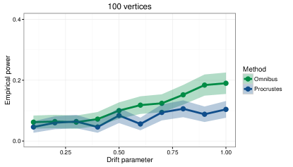
(c)

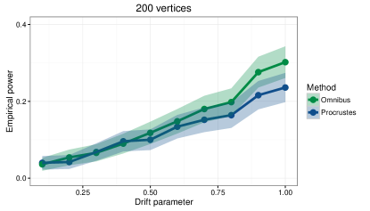
(d)

Figure 11: Power of the ASE-based (blue) and omnibus-based (green) tests to detect when the two graphs being testing differ in their latent positions. Subplots show power as a function of the drift parameter $\lambda$ for (a) $n=30$, (b) $n=50$, (c) $n=100$ and (d) $n=200$ vertices. Each point is the proportion of 500 trials for which the given technique correctly rejected the null hypothesis, and error bars denote two standard errors of this empirical mean.

6 Discussion and Conclusion

The omnibus embedding is a simple, scalable procedure for the simultaneous embedding of multiple graphs on the same vertex set, the output of which are multiple points in Euclidean space for each graph vertex. For a wide class of latent position random graphs, this embedding generates accurate estimates of latent positions and supplies empirical power for distinguishing when graphs are statistically different. Our consistency results in the $2\to\infty$ norm for the omnibus-derived estimates are competitive with state-of-the-art spectral approaches to latent position estimation, and our distributional results for the asymptotic normality of the rows of the omnibus embedding render principled the application of classical Euclidean inference techniques, such as analyses of variance, for the comparison of multiple population of graphs and the identification of drivers of graph similarity or difference at multiple scales, from whole graphs to subcommunities to vertices. We illustrate the utility of the omnibus embedding in data analyses of two different collections of noisy, weighted brain scans, and we uncover new insights into brain regions and vertices that are responsible for graph-level differences in two distinct data sets.

Further, we quantify the impact of multiple graphs on the variance of the rows of the embedding, specifically in relation to the variance given in Athreya et al. (2016). This result shows that as the number of graphs, $m$, grows, a significant reduction in the variance is achievable. Experimental data suggest that the omnibus embedding is competitive with state-of-the-art, multiple-graph spectral estimation of latent positions, and we surmise that the variance of the rows in the omnibus embedding is close to optimal for latent position estimators derived from the adjacency spectral embedding. That is, the variance of the omnibus embedding is asymptotically equal to the variance obtained by first averaging the $m$ graphs to get $\bar{\mathbf{A}}$ (which corresponds, in essence, to the maximum likelihood estimate for $\mathbf{P}$), and then performing an adjacency spectral embedding of $\bar{\mathbf{A}}$. Let $\hat{\mathbf{Z}}_{i}$ correspond to the $i$-th row of $\hat{\mathbf{Z}}=\operatorname{OMNI}(\mathbf{A}^{(1)},\mathbf{A}^{(2)},\dots,\mathbf{A}^{(m)},d)$, and let $\bar{\mathbf{X}}_{i}$ denote the $i$-th row of the adjacency spectral embedding of $\bar{\mathbf{A}}$. Let $\bar{\hat{\mathbf{Z}}}_{i}$ denote the average value of the $m$ rows of $\hat{\mathbf{Z}}$ corresponding to the $i$-th vertex, namely, the average of the $m$ vectors corresponding to the $i$-th vertex in the omnibus embedding. We conjecture that averaging the rows of the omnibus embedding accounts for all of the reduction in variance when one compares a single row of the omnibus embedding and a single row of $\bar{\mathbf{X}}$. Figure 9 provides weak evidence in favor of this conjecture, since it illustrates that the MSE of both the omnibus- and Procrustes-based estimates of the latent position estimates are very close to that of the estimate based on the mean adjacency matrix.

Conjecture 1.

(Decomposition of Variance) With notation as above, for large $n$,

$$\operatorname{Var}\left(\sqrt{n}\bar{\mathbf{X}}_{i}\right)\approx\operatorname{Var}\left(\sqrt{n}\bar{\hat{\mathbf{Z}}}_{i}\right)<\operatorname{Var}\left(\sqrt{n}\hat{\mathbf{Z}}_{i}\right).$$

We have also demonstrated that the omnibus embedding can be profitably deployed for two-sample semiparametric hypothesis testing of graph-valued data. Our omnibus embedding provides a natural mechanism for the simultaneous embedding of multiple graphs into a single vector space. This eliminates the need for multiple Procrustes alignments, which were required in previously-explored approaches to multiple-graph testing (Tang et al., 2017a). In the two-graph hypothesis testing framework of Tang et al. (2017a), each graph is embedded separately. Under the assumption of equality of latent positions (i.e., under $H_{0}$ in Equation  (8)), we note that embedding the first graph estimates the true latent positions $\mathbf{X}$ up to a unitary transformation in $\mathbb{R}^{d\times d}$. Call this estimate $\hat{\mathbf{X}}_{1}$. Similarly, $\hat{\mathbf{X}}_{2}$, the estimates based on the second graph, estimates $\mathbf{X}$ only up to some potentially different unitary rotation, i.e., $\hat{\mathbf{X}}_{2}\approx\mathbf{X}\mathbf{W}^{*}$ for some unitary $\mathbf{W}^{*}$. Procrustes alignment is thus required to discover the rotation aligning $\hat{\mathbf{X}}_{1}$ with $\hat{\mathbf{X}}_{2}$. In Tang et al. (2017a), it was shown that this Procrustes alignment, given by

$$\min_{\mathbf{W}\in\mathcal{O}_{d}}\|\hat{\mathbf{X}}_{1}-\hat{\mathbf{X}}_{2}\mathbf{W}\|_{F},$$ (10)

converges under the null hypothesis. The effect of this Procrustes alignment on subsequent inference is ill-understood. At the very least, it has the potential to introduce variance, and our simulations in Section 5 suggest that it negatively impacts performance in both estimation and testing settings. Furthermore, when the matrix $\mathbf{P}=\mathbf{X}\mathbf{X}^{T}$ does not have distinct eigenvalues (i.e., is not uniquely diagonalizable), this Procrustes step is unavoidable, since the difference $\|\hat{\mathbf{X}}_{1}-\hat{\mathbf{X}}_{2}\|_{F}$ need not converge at all.

In contrast, our omnibus embedding builds an alignment of the graphs into its very structure. To see this, consider, for simplicity, the $m=2$ case. Let $\mathbf{X}\in\mathbb{R}^{n\times d}$ be the matrix whose rows are the latent positions of both graphs $G_{1}$ and $G_{2}$, and let $\mathbf{M}\in\mathbb{R}^{2n\times 2n}$ be their omnibus matrix. Then

$$\mathbb{E}\mathbf{M}=\tilde{\mathbf{P}}=\begin{bmatrix}\mathbf{P}&\mathbf{P}\\ \mathbf{P}&\mathbf{P}\end{bmatrix}=\begin{bmatrix}\mathbf{X}\\ \mathbf{X}\end{bmatrix}\begin{bmatrix}\mathbf{X}\\ \mathbf{X}\end{bmatrix}^{T}.$$

Suppose now that we wish to factorize $\tilde{\mathbf{P}}$ as

$$\tilde{\mathbf{P}}=\begin{bmatrix}\mathbf{X}\\ \mathbf{X}\mathbf{W}^{*}\end{bmatrix}\begin{bmatrix}\mathbf{X}\\ \mathbf{X}\mathbf{W}^{*}\end{bmatrix}^{T}=\begin{bmatrix}\mathbf{P}&\mathbf{X}(\mathbf{W}^{*})^{T}\mathbf{X}^{T}\\ \mathbf{X}\mathbf{W}^{*}\mathbf{X}^{T}&\mathbf{P}\end{bmatrix}.$$

That is, we want to consider graphs $G_{1}$ and $G_{2}$ as being generated from the same latent positions, but in one case, say, under a different rotation. This possibility necessitates the Procrustes alignment in the case of separately-embedded graphs. In the case of the omnibus matrix, the structure of the $\tilde{\mathbf{P}}$ matrix implies that $\mathbf{W}^{*}=\mathbf{I}_{d}$. Thus, in contrast to the Procrustes alignment, the omnibus matrix incorporates an alignment a priori. Simulations show that the omnibus embedding outperforms the Procrustes-based test for equality of latent positions, especially in the case of moderately-sized graphs.

To further illustrate the utility of this omnibus embedding, consider the case of testing whether three different random dot product graphs have the same generating latent positions. The omnibus embedding gives us a single canonical representation of all three graphs: Let $\hat{\mathbf{X}}^{O}_{1}$, $\hat{\mathbf{X}}^{O}_{2}$, and $\hat{\mathbf{X}}^{O}_{3}$ be the estimates for the three latent position matrices generated from the omnibus embedding. To test whether any two of these random graphs have the same generating latent positions, we merely have to compare the Frobenius norms of their differences, as opposed to computing three separate Procrustes alignments. In the latter case, in effect, we do not have a canonical choice of coordinates in which to compare our graphs simultaneously.

In our analysis of BNU1 data, we “center” our omnibus matrix, by first considering $\mathbf{B}^{(i)}=\mathbf{A}^{(i)}-\bar{\mathbf{A}}$ and then performing an omnibus embedding on the $\mathbf{B}^{(i)}$ matrices. While our theorems are written for the uncentered case, the analysis of the centered version proceeds along similiar lines. We find that in many practical settings, centering meaningfully improves our ability to detect differences across graphs, and we offer the following conjectures as to why. First, we surmise that centering allows us to better assess covariance structure between estimated latent positions, and thereby improve clustering in a dissimilarity matrix. Second, centering can mitigate the effect of degree heterogeneity across graphs. Third, centering can dampen the potentially noisy impact of common subgraphs, if they exist, to more clearly address graph difference.

Investigating the impact of centering, both for theory and practice, is ongoing, and it is a prominent open problem in the analysis of the omnibus embedding. Of course, other open problems abound, such as an analysis of the omnibus embedding when the $m$ graphs are correlated, are weighted, or are corrupted by occlusion or noise; a closer examination of the impact of the Procrustes alignment on power; the development of an analogue to a Tukey test for determining which graphs differ when we test equality of multiple graphs; the comparative efficiency of the omnibus embedding relative to other spectral estimates; and finally, results for the omnibus embedding under the alternative, when the graph distributions are unequal. The elegance of the omnibus embedding, especially its anchoring in a long and robust history of spectral inference procedures, makes it an ideal point of departure for multiple graph inference, and the richness of the open problems it inspires suggests that the omnibus embedding will remain a key part of the graph statistician’s arsenal.

We collect here the technical proofs supporting our main result, Theorem 1. We consider the (transposed) $h$-th row of the matrix

$$\sqrt{n}\left(\mathbf{U}_{\mathbf{M}}\mathbf{S}_{\mathbf{M}}^{1/2}\mathbf{V}^{T}\mathbf{W}_{n}-\mathbf{U}_{\tilde{\mathbf{P}}}\mathbf{S}_{\tilde{\mathbf{P}}}^{1/2}\right),$$

where $\mathbf{V},\mathbf{W}_{n}\in\mathbb{R}^{d\times d}$ are orthogonal transformations. We follow the reasoning of Theorem 18 in Lyzinski et al. [2017], decomposing this matrix as $\sqrt{n}\left(\mathbf{U}_{\mathbf{M}}\mathbf{S}_{\mathbf{M}}^{1/2}\mathbf{V}^{T}\mathbf{W}_{n}-\mathbf{U}_{\tilde{\mathbf{P}}}\mathbf{S}_{\tilde{\mathbf{P}}}^{1/2}\right)=\sqrt{n}(\mathbf{N}+\mathbf{H})$, where $\mathbf{N},\mathbf{H}\in\mathbb{R}^{mn\times d}$. To prove our central limit theorem, we show that the (transposed) $h$-th row of $\sqrt{n}\mathbf{H}$ converges in probability to $\mathbf{0}$ and that the (transposed) $h$-th row of $\sqrt{n}\mathbf{N}$ converges in distribution to a mixture of normals. We note that Lemma 2, Observation 2, Lemma 3, Propositions 1 and 2, Lemma 4, and Lemma 5 provide the groundwork for establishing our consistency result, Lemma 1, and, thereafter, for showing that the $h$-th row of $\sqrt{n}\mathbf{H}$ converges in probability to $\mathbf{0}$. Next, Lemma 6 establishes that the $h$-th row of $\sqrt{n}\mathbf{N}$ converges in distribution to a mixture of normals; the proof of Theorem 1 then follows from Slutsky’s Theorem.

We begin with a standard matrix concentration inequality, reproduced from Tropp [2015].

Theorem 2.

[Matrix Bernstein; Tropp, 2015, Theorem 1.6.2] Consider independent random Hermitian matrices $\mathbf{H}^{(1)},\mathbf{H}^{(2)},\dots,\mathbf{H}^{(k)}\in\mathbb{R}^{n\times n}$ with $\mathbb{E}\mathbf{H}^{(i)}=\mathbf{0}$ and $\|\mathbf{H}^{(i)}\|\leq L$ with probability $1$ for all $i$ for some fixed $L>0$. Define $\mathbf{H}=\sum_{i=1}^{k}\mathbf{H}^{(i)}$, and let $v(\mathbf{H})=\|\mathbb{E}\mathbf{H}^{2}\|$. Then for all $t\geq 0$,

$$\Pr\left[\|\mathbf{H}\|\geq t\right]\leq 2n\exp\left\{\frac{-t^{2}/2}{v(\mathbf{H})+Lt/3}\right\}.$$

We will apply this matrix Bernstein inequality to the omnibus matrix to obtain a bound on $\|\mathbf{M}-\tilde{\mathbf{P}}\|$, from which it will follow by Weyl’s inequality [Horn and Johnson, 1985] that the eigenvalues of $\mathbf{M}$ are close to those of $\mathbb{E}\mathbf{M}$.

Lemma 2.

Let $\mathbf{M}\in\mathbb{R}^{mn\times mn}$ be the omnibus matrix of $\mathbf{A}^{(1)},\mathbf{A}^{(2)},\dots,\mathbf{A}^{(m)}$, where

$$(\mathbf{A}^{(1)},\mathbf{A}^{(2)},\dots,\mathbf{A}^{(m)},\mathbf{X})\sim\operatorname{JRDPG}(F,n,m).$$

Then $\|\mathbf{M}-\mathbb{E}\mathbf{M}\|\leq Cmn^{1/2}\log^{1/2}mn\text{ w.h.p. }$

Proof.

Condition on some $\mathbf{P}=\mathbf{X}\mathbf{X}^{T}$, so that

$$\mathbb{E}\mathbf{M}=\tilde{\mathbf{P}}=\begin{bmatrix}\mathbf{P}&\mathbf{P}&\dots&\mathbf{P}\\ \mathbf{P}&\mathbf{P}&\dots&\vdots\\ \vdots&\vdots&\ddots&\vdots\\ \mathbf{P}&\dots&\dots&\mathbf{P}\end{bmatrix}\in\mathbb{R}^{mn\times mn}.$$ (11)

We will apply Theorem 2 to $\mathbf{M}-\mathbb{E}\mathbf{M}$. For all $q\in[m]$ and $i,j\in[n]$, let $\mathbf{e}^{ij}=\mathbf{e}_{i}\mathbf{e}_{j}^{T}+\mathbf{e}_{j}\mathbf{e}_{i}^{T}$ and define block matrix $\mathbf{E}_{q,i,j}\in\mathbb{R}^{mn\times mn}$ with blocks of size $n$-by-$n$ by

$$\mathbf{E}_{q,i,j}=\begin{bmatrix}\mathbf{0}&\dots&\mathbf{0}&\mathbf{e}^{ij}&\mathbf{0}&\dots&\mathbf{0}\\ \mathbf{0}&\dots&\mathbf{0}&\mathbf{e}^{ij}&\mathbf{0}&\dots&\mathbf{0}\\ \vdots&\ddots&&\vdots&&&\vdots\\ \mathbf{0}&\dots&\mathbf{0}&\mathbf{e}^{ij}&\mathbf{0}&\dots&\mathbf{0}\\ \mathbf{e}^{ij}&\dots&\mathbf{e}^{ij}&2\mathbf{e}^{ij}&\mathbf{e}^{ij}&\dots&\mathbf{e}^{ij}\\ \mathbf{0}&\dots&\mathbf{0}&\mathbf{e}^{ij}&\mathbf{0}&\dots&0_{n}\\ \vdots&\ddots&&\vdots&&&\vdots\\ \mathbf{0}&\dots&\mathbf{0}&\mathbf{e}^{ij}&\mathbf{0}&\dots&\mathbf{0}\end{bmatrix},$$

where the $\mathbf{e}^{ij}$ terms appear in the $q$-th row and $q$-th column. Using this definition, we have

$$\mathbf{M}-\mathbb{E}\mathbf{M}=\sum_{q=1}^{m}\sum_{1\leq i<j\leq n}\frac{\mathbf{A}^{(q)}_{ij}-\mathbf{P}_{ij}}{2}\mathbf{E}_{q,i,j},$$

which is a sum of $m\binom{n}{2}$ independent zero-mean matrices, with $\left\|(\mathbf{A}^{(q)}_{ij}-\mathbf{P}_{ij})\mathbf{E}_{q,i,j}/2\right\|\leq\sqrt{m+1}$ for all $q\in[m]$ and $i,j\in[n]$.

To apply Theorem 2, it remains to consider the variance term $v(\mathbf{M}-\mathbb{E}\mathbf{M})$. We note first that, letting $\mathbf{D}_{ij}=\mathbf{e}_{i}\mathbf{e}_{i}^{T}+\mathbf{e}_{j}\mathbf{e}_{j}^{T}\in\mathbb{R}^{n\times n}$, we have

$$\mathbf{E}_{q,i,j}\mathbf{E}_{q,i,j}=\begin{bmatrix}\mathbf{D}_{ij}&\dots&\mathbf{D}_{ij}&\mathbf{D}_{ij}&\mathbf{D}_{ij}&\dots&\mathbf{D}_{ij}\\ \vdots&\ddots&\vdots&\vdots&\vdots&\ddots&\vdots\\ \mathbf{D}_{ij}&\dots&\mathbf{D}_{ij}&\mathbf{D}_{ij}&\mathbf{D}_{ij}&\dots&\mathbf{D}_{ij}\\ \mathbf{D}_{ij}&\dots&\mathbf{D}_{ij}&(m+3)\mathbf{D}_{ij}&\mathbf{D}_{ij}&\dots&\mathbf{D}_{ij}\\ \mathbf{D}_{ij}&\dots&\mathbf{D}_{ij}&\mathbf{D}_{ij}&\mathbf{D}_{ij}&\dots&\mathbf{D}_{ij}\\ \vdots&\ddots&\vdots&\vdots&\vdots&\ddots&\vdots\\ \mathbf{D}_{ij}&\dots&\mathbf{D}_{ij}&\mathbf{D}_{ij}&\mathbf{D}_{ij}&\dots&\mathbf{D}_{ij}\end{bmatrix},$$

where the $(m+3)\mathbf{D}_{ij}$ term appears in the $q$-th entry on the diagonal. Using the fact that the maximum row sum is an upper bound on the spectral norm [Horn and Johnson, 1985],

$$v(\mathbf{M}-\mathbb{E}\mathbf{M})=\left\|\sum_{q=1}^{m}\sum_{1\leq i<j\leq n}\frac{(\mathbf{A}^{(q)}_{ij}-\mathbf{P}_{ij})^{2}}{4}\mathbf{E}_{q,i,j}\mathbf{E}_{q,i,j}\right\|\leq\frac{(m+1)^{2}(n-1)}{4}.$$ (12)

Applying this upper bound on $v(\mathbf{M}-\mathbb{E}\mathbf{M})$ in Theorem 2, with $t=12(m+1)\sqrt{(n-1)\log mn}$, we obtain

$$\Pr\left[\|\mathbf{M}-\mathbb{E}\mathbf{M}\|\geq 12(m+1)\sqrt{(n-1)\log mn}\right]\leq 2m^{-3}n^{-2}.$$

Integrating over all $\mathbf{X}$ yields the result. ∎

Observation 1.

Let $\lambda_{1}\geq\lambda_{2}\geq\dots\geq\lambda_{d}>0$ denote the top $d$ eigenvalues of $\mathbf{P}=\mathbf{X}\mathbf{X}^{T}$, and let $\tilde{\mathbf{P}}$ be as in Equation (11). Then $\sigma(\tilde{\mathbf{P}})=\{m\lambda_{1},m\lambda_{2},\dots,m\lambda_{d},0,\dots,0\}$.

Proof.

This is immediate from the structure of $\tilde{\mathbf{P}}$, as defined in Equation (11). ∎

Observation 2.

Let $F$ be an inner product distribution on $\mathbb{R}^{d}$ with random vectors $\mathbf{X}_{1},\mathbf{X}_{2},\dots,\mathbf{X}_{n},\mathbf{Y}\stackrel{{\scriptstyle\text{i.i.d.}}}{{\sim}}F$. With probability at least $1-d^{2}/n^{2}$, it holds for all $i\in[d]$ that $|\lambda_{i}(\mathbf{P})-n\lambda_{i}(\mathbb{E}\mathbf{Y}\mathbf{Y}^{T})|\leq 2d\sqrt{n\log n}.$ Further, we have for all $i\in[d]$, $\lambda_{i}(\tilde{\mathbf{P}})\leq Cnm\delta$ with high probability.

Proof.

A slightly looser version of this bound appeared in Athreya et al. [2016]. We include a proof of this improved result for the sake of completeness.

Note that for $1\leq i\leq d$, we have $\lambda_{i}(\mathbf{P})=\lambda_{i}(\mathbf{X}\mathbf{X}^{T})=\lambda_{i}(\mathbf{X}^{T}\mathbf{X}).$ Hoeffding’s inequality applied to $(\mathbf{X}^{T}\mathbf{X}-n\mathbb{E}\mathbf{Y}\mathbf{Y}^{T})_{ij}=\sum_{t=1}^{n}(\mathbf{X}_{ti}\mathbf{X}_{tj}-\mathbb{E}\mathbf{Y}_{i}\mathbf{Y}_{j})$ yields, for all $i,j\in[d]$,

$$\Pr\left[|(\mathbf{X}^{T}\mathbf{X})-n\mathbb{E}\mathbf{Y}\mathbf{Y}^{T}|_{ij}\geq 2\sqrt{n\log n}\right]\leq\frac{2}{n^{2}}.$$

A union bound over all $i,j\in[d]$ implies that $\|\mathbf{X}^{T}\mathbf{X}-n\mathbb{E}\mathbf{Y}\mathbf{Y}^{T}\|_{F}^{2}\leq 4d^{2}n\log n$ with probability at least $1-2d^{2}/n^{2}$. Upper bounding the spectral norm by the Frobenius norm, we have $\|\mathbf{X}^{T}\mathbf{X}-n\mathbb{E}\mathbf{Y}\mathbf{Y}^{T}\|\leq 2d\sqrt{n\log n}$ with probability at least $1-2d^{2}/n^{2}$, and Weyl’s inequality [Horn and Johnson, 1985] thus implies $|\lambda_{i}(\mathbf{P})-n\lambda_{i}(\mathbb{E}\mathbf{Y}\mathbf{Y}^{T})|\leq 2d\sqrt{n\log n}$ for all $1\leq i\leq d$, from which Observation 1 and the reverse triangle inequality yield

$$\lambda_{i}(\tilde{\mathbf{P}})=m\lambda_{i}(\mathbf{P})\geq m\lambda_{d}(\mathbf{P})\geq m|n\lambda_{d}(\mathbb{E}\mathbf{Y}\mathbf{Y}^{T})-2d\sqrt{n\log n}|\geq Cmn$$

for suitably large $n$. ∎

The next several lemmas follow the reasoning in Lyzinski et al. [2017], in particular Proposition 16, Lemma 17 and Theorem 18, and thus they are stated here without proof.

Lemma 3.

[Adapted from Lyzinski et al., 2017, Prop. 16] Let $\tilde{\mathbf{P}}=\mathbf{U}_{\tilde{\mathbf{P}}}\mathbf{S}_{\tilde{\mathbf{P}}}\mathbf{U}_{\tilde{\mathbf{P}}}^{T}$ be the eigendecomposition of $\tilde{\mathbf{P}}$, where $\mathbf{U}_{\tilde{\mathbf{P}}}\in\mathbb{R}^{mn\times d}$ has orthonormal columns and $\mathbf{S}_{\tilde{\mathbf{P}}}\in\mathbb{R}^{d\times d}$ is diagonal and invertible. Let $\mathbf{S}_{\mathbf{M}}\in\mathbb{R}^{d\times d}$ be the diagonal matrix of the top $d$ eigenvalues of $\mathbf{M}$ and $\mathbf{U}_{\mathbf{M}}\in\mathbb{R}^{mn\times d}$ be the matrix with orthonormal columns containing the top $d$ corresponding eigenvectors, so that $\mathbf{U}_{\mathbf{M}}\mathbf{S}_{\mathbf{M}}\mathbf{U}_{\mathbf{M}}^{T}$ is our estimate of $\tilde{\mathbf{P}}$, as described above. Let $\mathbf{V}_{1}\mathbf{\Sigma}\mathbf{V}_{2}^{T}$ be the SVD of $\mathbf{U}_{\tilde{\mathbf{P}}}^{T}\mathbf{U}_{\mathbf{M}}$. Then

$$\|\mathbf{U}_{\tilde{\mathbf{P}}}^{T}\mathbf{U}_{\mathbf{M}}-\mathbf{V}_{1}\mathbf{V}_{2}^{T}\|_{F}\leq\frac{C\log mn}{n}\text{ w.h.p. }$$

It will be helpful to have the following two propositions, both of which follow from standard applications of Hoeffding’s inequality.

Proposition 1.

With notation as above,

$$\|\mathbf{U}_{\tilde{\mathbf{P}}}^{T}(\mathbf{M}-\tilde{\mathbf{P}})\|_{F}\leq C\sqrt{mn(m+\log mn)}\text{ w.h.p. }$$

Proposition 2.

With notation as above,

$$\|\mathbf{U}_{\tilde{\mathbf{P}}}^{T}(\mathbf{M}-\tilde{\mathbf{P}})\mathbf{U}_{\tilde{\mathbf{P}}}\|_{F}\leq C\sqrt{m\log mn}\text{ w.h.p. }$$

In what follows, we let $\mathbf{V}=\mathbf{V}_{1}\mathbf{V}_{2}^{T}$, where $\mathbf{V}_{1}$ and $\mathbf{V}_{2}$ are as defined in Lemma 3, i.e., $\mathbf{V}_{1}\mathbf{\Sigma}\mathbf{V}_{2}^{T}$ is the SVD of $\mathbf{U}_{\tilde{\mathbf{P}}}^{T}\mathbf{U}_{\mathbf{M}}$. The following lemma shows that the matrix $\mathbf{V}$ “approximately commutes” with several diagonal matrices that will be of import in later computations.

Lemma 4.

[Adapted from Lyzinski et al., 2017, Lemma 17] Let $\mathbf{V}=\mathbf{V}_{1}\mathbf{V}_{2}^{T}$ be as defined above. Then

$$\|\mathbf{V}\mathbf{S}_{\mathbf{M}}-\mathbf{S}_{\tilde{\mathbf{P}}}\mathbf{V}\|_{F}\leq Cm\log mn\text{ w.h.p. },$$ (13)

$$\|\mathbf{V}\mathbf{S}_{\mathbf{M}}^{1/2}-\mathbf{S}_{\tilde{\mathbf{P}}}^{1/2}\mathbf{V}\|_{F}\leq\frac{Cm^{1/2}\log mn}{n^{1/2}}\text{ w.h.p. }$$ (14)

and

$$\|\mathbf{V}\mathbf{S}_{\mathbf{M}}^{-1/2}-\mathbf{S}_{\tilde{\mathbf{P}}}^{-1/2}\mathbf{V}\|_{F}\leq C(mn)^{-3/2}\text{ w.h.p. }$$ (15)

To prove our central limit theorem, we require somewhat more precise control on certain residual terms, which we establish in the following key lemma.

Lemma 5.

Define

$$\mathbf{R}_{1} =\mathbf{U}_{\tilde{\mathbf{P}}}\mathbf{U}_{\tilde{\mathbf{P}}}^{T}\mathbf{U}_{\mathbf{M}}-\mathbf{U}_{\tilde{\mathbf{P}}}\mathbf{V}$$

$$\mathbf{R}_{2} =\mathbf{V}\mathbf{S}_{\mathbf{M}}^{1/2}-\mathbf{S}_{\tilde{\mathbf{P}}}^{1/2}\mathbf{V}$$

$$\mathbf{R}_{3} =\mathbf{U}_{\mathbf{M}}-\mathbf{U}_{\tilde{\mathbf{P}}}\mathbf{U}_{\tilde{\mathbf{P}}}^{T}\mathbf{U}_{\mathbf{M}}+\mathbf{R}_{1}=\mathbf{U}_{\mathbf{M}}-\mathbf{U}_{\tilde{\mathbf{P}}}\mathbf{V}.$$

Then the following convergences in probability hold:

$$\sqrt{n}\left[(\mathbf{M}-\tilde{\mathbf{P}})\mathbf{U}_{\tilde{\mathbf{P}}}(\mathbf{V}\mathbf{S}_{\mathbf{M}}^{-1/2}-\mathbf{S}_{\tilde{\mathbf{P}}}^{-1/2}\mathbf{V})\right]_{h}\xrightarrow{P}\mathbf{0},$$ (16)

$$\sqrt{n}\left[\mathbf{U}_{\tilde{\mathbf{P}}}\mathbf{U}_{\tilde{\mathbf{P}}}^{T}(\mathbf{M}-\tilde{\mathbf{P}})\mathbf{U}_{\tilde{\mathbf{P}}}\mathbf{V}\mathbf{S}_{\mathbf{M}}^{-1/2}\right]_{h}\xrightarrow{P}\mathbf{0},$$ (17)

$$\sqrt{n}\left[(\mathbf{I}-\mathbf{U}_{\tilde{\mathbf{P}}}\mathbf{U}_{\tilde{\mathbf{P}}}^{T})(\mathbf{M}-\tilde{\mathbf{P}})\mathbf{R}_{3}\mathbf{S}_{\mathbf{M}}^{-1/2}\right]_{h}\xrightarrow{P}\mathbf{0},$$ (18)

and with high probability,

$$\|\mathbf{R}_{1}\mathbf{S}_{\mathbf{M}}^{1/2}+\mathbf{U}_{\tilde{\mathbf{P}}}\mathbf{R}_{2}\|_{F}\leq\frac{Cm^{1/2}\log mn}{n^{1/2}}.$$

Proof.

We begin by observing that

$$\|\mathbf{R}_{1}\mathbf{S}_{\mathbf{M}}^{1/2}+\mathbf{U}_{\tilde{\mathbf{P}}}\mathbf{R}_{2}\|_{F}\leq\|\mathbf{R}_{1}\|_{F}\|\mathbf{S}_{\mathbf{M}}^{1/2}\|+\|\mathbf{R}_{2}\|_{F}.$$

Lemma 3 and the trivial upper bound on the eigenvalues of $\mathbf{M}$ ensures that

$$\|\mathbf{R}_{1}\|_{F}\|\mathbf{S}_{\mathbf{M}}^{1/2}\|\leq\frac{Cm^{1/2}\log mn}{n^{1/2}}\text{ w.h.p. },$$

Combining this with Equation (14), we conclude that

$$\|\mathbf{R}_{1}\mathbf{S}_{\mathbf{M}}^{1/2}+\mathbf{U}_{\tilde{\mathbf{P}}}\mathbf{R}_{2}\|_{F}\leq\frac{Cm^{1/2}\log mn}{n^{1/2}}\text{ w.h.p. }$$

We will establish (16), (17) and (18) order. To see (16), observe that

$$\sqrt{n}\|(\mathbf{M}-\tilde{\mathbf{P}})\mathbf{U}_{\tilde{\mathbf{P}}}(\mathbf{V}\mathbf{S}_{\mathbf{M}}^{-1/2}-\mathbf{S}_{\tilde{\mathbf{P}}}^{-1/2}\mathbf{V})\|_{F}\leq\sqrt{n}\|(\mathbf{M}-\tilde{\mathbf{P}})\mathbf{U}_{\tilde{\mathbf{P}}}\|\|\mathbf{V}\mathbf{S}_{\mathbf{M}}^{-1/2}-\mathbf{S}_{\tilde{\mathbf{P}}}^{-1/2}\mathbf{V}\|_{F},$$

and application of Proposition 1 and Lemma 4 imply that with high probability

$$\sqrt{n}\|(\mathbf{M}-\tilde{\mathbf{P}})\mathbf{U}_{\tilde{\mathbf{P}}}(\mathbf{V}\mathbf{S}_{\mathbf{M}}^{-1/2}-\mathbf{S}_{\tilde{\mathbf{P}}}^{-1/2}\mathbf{V})\|_{F}\leq C\sqrt{\frac{\log mn}{mn^{3}}},$$

which goes to $0$ as $n\rightarrow\infty$.

To show the convergence in (17), we recall that $\mathbf{U}_{\tilde{\mathbf{P}}}\mathbf{S}_{\tilde{\mathbf{P}}}^{1/2}=\mathbf{Z}\mathbf{W}^{T}$, and observe that since the rows of the latent position matrix $\mathbf{Z}$ are necessarily bounded in Euclidean norm by $1$, and since the top $d$ eigenvalues of $\tilde{\mathbf{P}}$ are of order $mn$, it follows that

$$\|\mathbf{U}_{\tilde{\mathbf{P}}}\|_{2\rightarrow\infty}\leq C(mn)^{-1/2}\text{ w.h.p. }$$ (19)

Next, Proposition 2 and Observation 2 imply that

$$\|(\mathbf{U}_{\tilde{\mathbf{P}}}\mathbf{U}_{\tilde{\mathbf{P}}}^{T}(\mathbf{M}-\tilde{\mathbf{P}})\mathbf{U}_{\tilde{\mathbf{P}}}\mathbf{V}\mathbf{S}_{\mathbf{M}}^{-1/2})_{h}\| \leq\|\mathbf{U}_{\tilde{\mathbf{P}}}\|_{2\rightarrow\infty}\|\mathbf{U}_{\tilde{\mathbf{P}}}^{T}(\mathbf{M}-\tilde{\mathbf{P}})\mathbf{U}_{\tilde{\mathbf{P}}}\|\|\mathbf{S}_{\mathbf{M}}^{-1/2}\|$$

$$\leq\frac{C\log^{1/2}mn}{m^{1/2}n}\text{ w.h.p.},$$

which implies (17).

Finally, to establish (18), we must bound the Euclidean norm of the vector

$$\left[(\mathbf{I}-\mathbf{U}_{\tilde{\mathbf{P}}}\mathbf{U}_{\tilde{\mathbf{P}}}^{T})(\mathbf{M}-\tilde{\mathbf{P}})\mathbf{R}_{3}\mathbf{S}_{\mathbf{M}}^{-1/2}\right]_{h},$$ (20)

where, as defined above, $\mathbf{R}_{3}=\mathbf{U}_{\mathbf{M}}-\mathbf{U}_{\tilde{\mathbf{P}}}\mathbf{V}$. Let $\mathbf{B}_{1}$ and $\mathbf{B}_{2}$ be defined as follows:

$$\mathbf{B}_{1} =(\mathbf{I}-\mathbf{U}_{\tilde{\mathbf{P}}}\mathbf{U}_{\tilde{\mathbf{P}}}^{T})(\mathbf{M}-\tilde{\mathbf{P}})(\mathbf{I}-\mathbf{U}_{\tilde{\mathbf{P}}}\mathbf{U}_{\tilde{\mathbf{P}}}^{T})\mathbf{U}_{\mathbf{M}}\mathbf{S}_{\mathbf{M}}^{-1/2}$$ (21)

$$\mathbf{B}_{2} =(\mathbf{I}-\mathbf{U}_{\tilde{\mathbf{P}}}\mathbf{U}_{\tilde{\mathbf{P}}}^{T})(\mathbf{M}-\tilde{\mathbf{P}})\mathbf{U}_{\tilde{\mathbf{P}}}(\mathbf{U}_{\tilde{\mathbf{P}}}^{T}\mathbf{U}_{\mathbf{M}}-\mathbf{V})\mathbf{S}_{\mathbf{M}}^{-1/2}$$

Recalling that $\mathbf{R}_{3}=\mathbf{U}_{\mathbf{M}}-\mathbf{U}_{\tilde{\mathbf{P}}}\mathbf{V}$, we have

$$(\mathbf{I}-\mathbf{U}_{\tilde{\mathbf{P}}}\mathbf{U}_{\tilde{\mathbf{P}}}^{T})(\mathbf{M}-\tilde{\mathbf{P}})\mathbf{R}_{3}\mathbf{S}_{\mathbf{M}}^{-1/2} =(\mathbf{I}-\mathbf{U}_{\tilde{\mathbf{P}}}\mathbf{U}_{\tilde{\mathbf{P}}}^{T})(\mathbf{M}-\tilde{\mathbf{P}})(\mathbf{U}_{\mathbf{M}}-\mathbf{U}_{\tilde{\mathbf{P}}}\mathbf{U}_{\tilde{\mathbf{P}}}^{T}\mathbf{U}_{\mathbf{M}})\mathbf{S}_{\mathbf{M}}^{-1/2}$$

$$~{}~{}~{}~{}~{}~{}+(\mathbf{I}-\mathbf{U}_{\tilde{\mathbf{P}}}\mathbf{U}_{\tilde{\mathbf{P}}}^{T})(\mathbf{M}-\tilde{\mathbf{P}})(\mathbf{U}_{\tilde{\mathbf{P}}}\mathbf{U}_{\tilde{\mathbf{P}}}^{T}\mathbf{U}_{\mathbf{M}}-\mathbf{U}_{\tilde{\mathbf{P}}}\mathbf{V})\mathbf{S}_{\mathbf{M}}^{-1/2}$$

$$=\mathbf{B}_{1}+\mathbf{B}_{2}.$$

We will bound the Euclidean norm of the $h$-th row of each of these two matrices on the right-hand side, from which a triangle inequality will yield our desired bound on the quantity in Equation (20). Recall that we use $C$ to denote a positive constant, independent of $n$ and $m$, which may change from line to line.

Let us first consider $\mathbf{B}_{2}=(\mathbf{I}-\mathbf{U}_{\tilde{\mathbf{P}}}\mathbf{U}_{\tilde{\mathbf{P}}}^{T})(\mathbf{M}-\tilde{\mathbf{P}})\mathbf{U}_{\tilde{\mathbf{P}}}(\mathbf{U}_{\tilde{\mathbf{P}}}^{T}\mathbf{U}_{\mathbf{M}}-\mathbf{V})\mathbf{S}_{\mathbf{M}}^{-1/2}$. We have

$$\|\mathbf{B}_{2}\|_{F}\leq\|(\mathbf{I}-\mathbf{U}_{\tilde{\mathbf{P}}}\mathbf{U}_{\tilde{\mathbf{P}}}^{T})(\mathbf{M}-\tilde{\mathbf{P}})\mathbf{U}_{\tilde{\mathbf{P}}}\|\|\mathbf{U}_{\tilde{\mathbf{P}}}^{T}\mathbf{U}_{\mathbf{M}}-\mathbf{V}\|_{F}\|\mathbf{S}_{\mathbf{M}}^{-1/2}\|.$$

By submultiplicativity of the spectral norm and Lemma 2, $\|(\mathbf{I}-\mathbf{U}_{\tilde{\mathbf{P}}}\mathbf{U}_{\tilde{\mathbf{P}}}^{T})(\mathbf{M}-\tilde{\mathbf{P}})\mathbf{U}_{\tilde{\mathbf{P}}}\|\leq Cmn^{1/2}\log^{1/2}mn$ with high probability. From Lemma 3 and Observation 2, respectively, we have with high probability

$$\|\mathbf{U}_{\tilde{\mathbf{P}}}^{T}\mathbf{U}_{\mathbf{M}}-\mathbf{V}\|_{F}\leq Cn^{-1}\log mn\enspace\text{ and }\enspace\|\mathbf{S}_{\mathbf{M}}^{-1/2}\|\leq C(mn)^{-1/2}$$

Thus, we deduce that with high probability,

$$\|\mathbf{B}_{2}\|_{F}\leq\frac{Cm^{1/2}\log^{3/2}mn}{n}$$ (22)

from which it follows that $\|\sqrt{n}\mathbf{B}_{2}\|_{F}\xrightarrow{P}0$, and hence $\|\sqrt{n}(\mathbf{B}_{2})_{h}\|\xrightarrow{P}0$.

Turning our attention to $\mathbf{B}_{1}$, and recalling that $\mathbf{U}_{\mathbf{M}}^{T}\mathbf{U}_{\mathbf{M}}=I$, we note that

$$\|(\mathbf{B}_{1})_{h}\| =\left\|\left[(\mathbf{I}-\mathbf{U}_{\tilde{\mathbf{P}}}\mathbf{U}_{\tilde{\mathbf{P}}}^{T})(\mathbf{M}-\tilde{\mathbf{P}})(\mathbf{I}-\mathbf{U}_{\tilde{\mathbf{P}}}\mathbf{U}_{\tilde{\mathbf{P}}}^{T})\mathbf{U}_{\mathbf{M}}\mathbf{S}_{\mathbf{M}}^{-1/2}\right]_{h}\right\|$$

$$=\left\|\left[(\mathbf{I}-\mathbf{U}_{\tilde{\mathbf{P}}}\mathbf{U}_{\tilde{\mathbf{P}}}^{T})(\mathbf{M}-\tilde{\mathbf{P}})(I-\mathbf{U}_{\tilde{\mathbf{P}}}\mathbf{U}_{\tilde{\mathbf{P}}}^{T})\mathbf{U}_{\mathbf{M}}\mathbf{U}_{\mathbf{M}}^{T}\mathbf{U}_{\mathbf{M}}\mathbf{S}_{\mathbf{M}}^{-1/2}\right]_{h}\right\|$$

$$\leq\left\|\mathbf{U}_{\mathbf{M}}\mathbf{S}_{\mathbf{M}}^{-1/2}\right\|\left\|\left[(\mathbf{I}-\mathbf{U}_{\tilde{\mathbf{P}}}\mathbf{U}_{\tilde{\mathbf{P}}}^{T})(\mathbf{M}-\tilde{\mathbf{P}})(\mathbf{I}-\mathbf{U}_{\tilde{\mathbf{P}}}\mathbf{U}_{\tilde{\mathbf{P}}}^{T})\mathbf{U}_{\mathbf{M}}\mathbf{U}_{\mathbf{M}}^{T}\right]_{h}\right\|.$$

Let $\epsilon>0$ be a constant. We will show that

$$\lim_{n\rightarrow\infty}\Pr\left[\|\sqrt{n}(\mathbf{B}_{1})_{h}\|>\epsilon\right]=0.$$ (23)

For ease of notation, define

$$\mathbf{E}_{1}=(\mathbf{I}-\mathbf{U}_{\tilde{\mathbf{P}}}\mathbf{U}_{\tilde{\mathbf{P}}}^{T})(\mathbf{M}-\tilde{\mathbf{P}})(\mathbf{I}-\mathbf{U}_{\tilde{\mathbf{P}}}\mathbf{U}_{\tilde{\mathbf{P}}}^{T})\mathbf{U}_{\mathbf{M}}\mathbf{U}_{\mathbf{M}}^{T}.$$

We will show that

$$\lim_{n\rightarrow\infty}\Pr\left[\sqrt{n}\left\|\left[\mathbf{E}_{1}\right]_{h}\right\|>n^{1/4}\right]=0,$$ (24)

which will imply (23) since, by Observation 2,

$$\|\mathbf{U}_{\mathbf{M}}\mathbf{S}_{\mathbf{M}}^{-1/2}\|\leq C(mn)^{-1/2}\text{ w.h.p. }$$

We verify the bound in (24) by showing that the Frobenius norms of the rows of $\mathbf{E}_{1}$ are exchangeable, and thus all of these Frobenius norms have the same expectation. We can then invoke Markov’s inequality to bound the probability that the Frobenius norm of any fixed row exceeds a specified threshold.

To prove exchangeability of the Frobenius norms of the rows of $\mathbf{E}_{1}$, note that if $\mathbf{Q}\in\mathbb{R}^{mn\times mn}$ is any permutation matrix, right multiplication of an $mn\times mn$ matrix ${\bf G}$ by $\mathbf{Q}^{T}$ merely permutes the columns of ${\bf G}$; hence the Frobenius norm of the $i$-th row of $\mathbf{Q}{\bf G}\mathbf{Q}^{T}$ is the same as the Frobenius norm of the $i$-th row of $\mathbf{Q}{\bf G}$.

For any $n\times n$ matrix real symmetric matrix ${\bf G}$, let $\mathcal{P}_{d}({\bf G})$ denote the projection onto the eigenspace defined by the top $d$ eigenvalues (in magnitude) of ${\bf G}$. Similarly, let $\mathcal{P}_{d}^{\perp}({\bf G})$ denote the projection onto the orthogonal complement of that eigenspace. For the matrix $\tilde{\mathbf{P}}$, for example, the columns of $\mathbf{U}_{\tilde{\mathbf{P}}}$ are a basis for the eigenspace associated to the top $d$ eigenvalues, and the matrix $\mathbf{U}_{\tilde{\mathbf{P}}}\mathbf{U}_{\tilde{\mathbf{P}}}^{T}$ is the unique projection operator into this eigenspace.

Observe that

$$\mathbf{Q}\mathbf{U}_{\tilde{\mathbf{P}}}\mathbf{U}_{\tilde{\mathbf{P}}}^{T}\mathbf{Q}^{T}\mathbf{Q}\tilde{\mathbf{P}}\mathbf{Q}^{T}=\mathbf{Q}\mathbf{U}_{\tilde{\mathbf{P}}}\mathbf{U}_{\tilde{\mathbf{P}}}^{T}\tilde{\mathbf{P}}\mathbf{Q}^{T},$$

and thus $\mathbf{Q}\mathbf{U}_{\tilde{\mathbf{P}}}\mathbf{U}_{\tilde{\mathbf{P}}}^{T}\mathbf{Q}^{T}$ is the projection matrix onto the eigenspace of top $d$ eigenvalues of $\mathbf{Q}\tilde{\mathbf{P}}\mathbf{Q}^{T}$ if and only if $\mathbf{U}_{\tilde{\mathbf{P}}}\mathbf{U}_{\tilde{\mathbf{P}}}^{T}$ is the corresponding projection matrix for $\tilde{\mathbf{P}}$. Similarly, $\mathbf{U}_{\mathbf{M}}\mathbf{U}_{\mathbf{M}}^{T}$ is the unique projection operator onto the eigenspace defined by the top $d$ eigenvalues (in magnitude) of $\mathbf{M}$, and $\mathbf{Q}\mathbf{U}_{\mathbf{M}}\mathbf{U}_{\mathbf{M}}^{T}\mathbf{Q}^{T}$ is the corresponding projection matrix for $\mathbf{Q}\mathbf{M}\mathbf{Q}^{T}$.

Now, for any pair of $n\times n$ matrices $({\bf G},{\bf H})$, let $\mathcal{L}({\bf G},{\bf H})$ represent the following operator:

$$\mathcal{L}({\bf G},{\bf H})=\mathcal{P}_{d}^{\perp}({\bf G})({\bf G}-{\bf H})\mathcal{P}_{d}^{\perp}({\bf G})\mathcal{P}_{d}({\bf H})$$

We see that $\mathcal{L}(\mathbf{M},\tilde{\mathbf{P}})=\mathbf{E}_{1}$, and by uniqueness of projections, we note that

$$\mathcal{L}(\mathbf{Q}\mathbf{M}\mathbf{Q}^{T},\mathbf{Q}\tilde{\mathbf{P}}\mathbf{Q}^{T})$$ (25)

$$=(\mathbf{Q}(\mathbf{I}-\mathbf{U}_{\mathbf{P}}\mathbf{U}_{\tilde{\mathbf{P}}}^{T})\mathbf{Q}^{T}\mathbf{Q}(\mathbf{M}-\tilde{\mathbf{P}})\mathbf{Q}^{T}\mathbf{Q}(\mathbf{I}-\mathbf{U}_{\tilde{\mathbf{P}}}\mathbf{U}_{\tilde{\mathbf{P}}}^{T})\mathbf{Q}^{T}\mathbf{Q}(\mathbf{U}_{\mathbf{M}}\mathbf{U}_{\mathbf{M}}^{T})\mathbf{Q}^{T}$$ (26)

$$=\mathbf{Q}\mathbf{E}_{1}\mathbf{Q}^{T}$$ (27)

Since we assume that the latent positions for our graphs are i.i.d, the entries of the matrix pair $(\mathbf{M},\tilde{\mathbf{P}})$ have the same joint distribution as the entries of the pair $(\mathbf{Q}\mathbf{M}\mathbf{Q}^{T},\mathbf{Q}\tilde{\mathbf{P}}\mathbf{Q}^{T})$. Therefore, the entries of the matrix $\mathcal{L}(\mathbf{M},\tilde{\mathbf{P}})$ have the same distribution as those of $\mathcal{L}(\mathbf{Q}\mathbf{M}\mathbf{Q}^{T},\mathbf{Q}\tilde{\mathbf{P}}\mathbf{Q}^{T})$. By Eq. (25), this implies that $\mathbf{E}_{1}$ has the same distribution as $\mathbf{Q}\mathbf{E}_{1}\mathbf{Q}^{T}$. Since the Frobenius norm of any row of $\mathbf{Q}\mathbf{E}_{1}\mathbf{Q}^{T}$ is exactly equal to the Frobenius norm of the corresponding to row of $\mathbf{Q}\mathbf{E}_{1}$, we conclude that the Frobenius norms of rows of $\mathbf{E}_{1}$ have the same distribution as the Frobenius norms of the rows of $\mathbf{Q}\mathbf{E}_{1}$, thereby establishing that the Frobenius norms of the rows of $\mathbf{E}_{1}$ are exchangeable. This row-exchangeability for the Frobenius norms of $\mathbf{E}_{1}$ implies that each row has the same expectation, and hence $mn\mathbb{E}\|(\mathbf{E}_{1})_{h}\|^{2}=\mathbb{E}\|\mathbf{E}_{1}\|_{F}^{2}$. Applying Markov’s inequality,

$$\Pr\left[\left\|\sqrt{n}\left[\mathbf{E}_{1}\right]_{h}\right\|>t\right] \leq\frac{n\mathbb{E}\left\|\left[(\mathbf{I}-\mathbf{U}_{\tilde{\mathbf{P}}}\mathbf{U}_{\tilde{\mathbf{P}}}^{T})(\mathbf{M}-\tilde{\mathbf{P}})(\mathbf{I}-\mathbf{U}_{\tilde{\mathbf{P}}}\mathbf{U}_{\tilde{\mathbf{P}}}^{T})\mathbf{U}_{\mathbf{M}}\mathbf{U}_{\mathbf{M}}^{T}\right]_{h}\right\|^{2}}{t^{2}}$$ (28)

$$=\frac{\mathbb{E}\left\|(\mathbf{I}-\mathbf{U}_{\tilde{\mathbf{P}}}\mathbf{U}_{\tilde{\mathbf{P}}}^{T})(\mathbf{M}-\tilde{\mathbf{P}})(\mathbf{I}-\mathbf{U}_{\tilde{\mathbf{P}}}\mathbf{U}_{\tilde{\mathbf{P}}}^{T})\mathbf{U}_{\mathbf{M}}\mathbf{U}_{\mathbf{M}}^{T}\right\|_{F}^{2}}{mt^{2}}.$$

We will proceed by showing that with high probability,

$$\left\|(\mathbf{I}-\mathbf{U}_{\tilde{\mathbf{P}}}\mathbf{U}_{\tilde{\mathbf{P}}}^{T})(\mathbf{M}-\tilde{\mathbf{P}})(\mathbf{I}-\mathbf{U}_{\tilde{\mathbf{P}}}\mathbf{U}_{\tilde{\mathbf{P}}}^{T})\mathbf{U}_{\mathbf{M}}\mathbf{U}_{\mathbf{M}}^{T}\right\|_{F}\leq Cm\log mn,$$ (29)

whence choosing $t=n^{1/4}$ in (28) yields that

$$\lim_{n\rightarrow\infty}\Pr\left[\left\|\sqrt{n}\left[(\mathbf{I}-\mathbf{U}_{\tilde{\mathbf{P}}}\mathbf{U}_{\tilde{\mathbf{P}}}^{T})(\mathbf{M}-\tilde{\mathbf{P}})(\mathbf{I}-\mathbf{U}_{\tilde{\mathbf{P}}}\mathbf{U}_{\tilde{\mathbf{P}}}^{T})\mathbf{U}_{\mathbf{M}}\mathbf{U}_{\mathbf{M}}^{T}\right]_{h}\right\|>n^{1/4}\right]=0,$$

and (23) will follow. We have

$$\left\|(\mathbf{I}-\mathbf{U}_{\tilde{\mathbf{P}}}\mathbf{U}_{\tilde{\mathbf{P}}}^{T})(\mathbf{M}-\tilde{\mathbf{P}})(\mathbf{I}-\mathbf{U}_{\tilde{\mathbf{P}}}\mathbf{U}_{\tilde{\mathbf{P}}}^{T})\mathbf{U}_{\mathbf{M}}\mathbf{U}_{\mathbf{M}}^{T}\right\|_{F}\leq\|\mathbf{M}-\tilde{\mathbf{P}}\|\|\mathbf{U}_{\mathbf{M}}-\mathbf{U}_{\tilde{\mathbf{P}}}\mathbf{U}_{\tilde{\mathbf{P}}}^{T}\mathbf{U}_{\mathbf{M}}\|_{F}\|\mathbf{U}_{\mathbf{M}}\|$$

Theorem 2 implies that the first term in this product is at most $Cmn^{1/2}\log^{1/2}mn$ with high probability, and the final term in this product is, trivially, at most $1$. To bound the second term, we will follow reasoning similar to that in Lemma 4, combined with the Davis-Kahan theorem. The Davis-Kahan Theorem [Davis and Kahan, 1970, Bhatia, 1997] implies that for a suitable constant $C>0$,

$$\|\mathbf{U}_{\mathbf{M}}\mathbf{U}_{\mathbf{M}}^{T}-\mathbf{U}_{\tilde{\mathbf{P}}}\mathbf{U}_{\tilde{\mathbf{P}}}^{T}\|\leq\frac{C\|\mathbf{M}-\tilde{\mathbf{P}}\|}{\lambda_{d}(\tilde{\mathbf{P}})}.$$

By Theorem 2 in Yu et al. [2015], there exists orthonormal $\mathbf{W}\in\mathbb{R}^{d\times d}$ such that

$$\|\mathbf{U}_{\mathbf{M}}-\mathbf{U}_{\tilde{\mathbf{P}}}\mathbf{W}\|_{F}\leq C\|\mathbf{U}_{\mathbf{M}}\mathbf{U}_{\mathbf{M}}^{T}-\mathbf{U}_{\tilde{\mathbf{P}}}\mathbf{U}_{\tilde{\mathbf{P}}}^{T}\|_{F}.$$

We observe further that the multivariate linear least squares problem

$$\min_{\mathbf{T}\in\mathbb{R}^{d\times d}}\|\mathbf{U}_{\mathbf{M}}-\mathbf{U}_{\tilde{\mathbf{P}}}\mathbf{T}\|_{F}^{2}$$

is solved by $\mathbf{T}=\mathbf{U}_{\tilde{\mathbf{P}}}^{T}\mathbf{U}_{\mathbf{M}}$. Thus, combining all of the above,

$$\|\mathbf{U}_{\mathbf{M}}-\mathbf{U}_{\tilde{\mathbf{P}}}\mathbf{U}_{\tilde{\mathbf{P}}}^{T}\mathbf{U}_{\mathbf{M}}\|_{F}^{2} \leq\|\mathbf{U}_{\mathbf{M}}-\mathbf{U}_{\tilde{\mathbf{P}}}\mathbf{W}\|_{F}^{2}\leq C\|\mathbf{U}_{\mathbf{M}}\mathbf{U}_{\mathbf{M}}^{T}-\mathbf{U}_{\tilde{\mathbf{P}}}\mathbf{U}_{\tilde{\mathbf{P}}}^{T}\|_{F}^{2}$$

$$\leq C\|\mathbf{U}_{\mathbf{M}}\mathbf{U}_{\mathbf{M}}^{T}-\mathbf{U}_{\tilde{\mathbf{P}}}\mathbf{U}_{\tilde{\mathbf{P}}}^{T}\|^{2}\leq\frac{C\|\mathbf{M}-\tilde{\mathbf{P}}\|}{\lambda_{d}(\tilde{\mathbf{P}})}\leq\frac{C\log^{1/2}mn}{n^{1/2}}\enspace\text{ w.h.p. }$$

Thus, we have

$$\left\|(\mathbf{I}-\mathbf{U}_{\tilde{\mathbf{P}}}\mathbf{U}_{\tilde{\mathbf{P}}}^{T})(\mathbf{M}-\tilde{\mathbf{P}})(\mathbf{I}-\mathbf{U}_{\tilde{\mathbf{P}}}\mathbf{U}_{\tilde{\mathbf{P}}}^{T})\mathbf{U}_{\mathbf{M}}\mathbf{U}_{\mathbf{M}}^{T}\right\|_{F} \leq\|\mathbf{M}-\tilde{\mathbf{P}}\|\|\mathbf{U}_{\mathbf{M}}-\mathbf{U}_{\tilde{\mathbf{P}}}\mathbf{U}_{\tilde{\mathbf{P}}}^{T}\mathbf{U}_{\mathbf{M}}\|\|\mathbf{U}_{\mathbf{M}}\|_{F}$$

$$\leq Cm\log mn\text{ w.h.p. },$$

which implies (29), as required, and thus the convergence in (18) is established, completing the proof. ∎

We are now ready to prove Lemma 1 on the consistency of the omnibus embedding; that is, we can now prove that there exists an orthogonal matrix $\tilde{\mathbf{W}}\in\mathbb{R}^{d\times d}$ such that with high probability,

$$\|\mathbf{U}_{\mathbf{M}}\mathbf{S}_{\mathbf{M}}^{1/2}-\mathbf{U}_{\tilde{\mathbf{P}}}\mathbf{S}_{\tilde{\mathbf{P}}}^{1/2}\tilde{\mathbf{W}}\|_{2\rightarrow\infty}\leq\frac{Cm^{1/2}\log mn}{\sqrt{n}}.$$

Proof of Lemma 1.

Observe that

$$\mathbf{U}_{\mathbf{M}}\mathbf{S}_{\mathbf{M}}^{1/2}-\mathbf{U}_{\tilde{\mathbf{P}}}\mathbf{S}_{\tilde{\mathbf{P}}}^{1/2}\mathbf{V} =(\mathbf{M}-\tilde{\mathbf{P}})\mathbf{U}_{\tilde{\mathbf{P}}}\mathbf{S}_{\tilde{\mathbf{P}}}^{-1/2}\mathbf{V}+(\mathbf{M}-\tilde{\mathbf{P}})\mathbf{U}_{\tilde{\mathbf{P}}}(\mathbf{V}\mathbf{S}_{\mathbf{M}}^{-1/2}-\mathbf{S}_{\tilde{\mathbf{P}}}^{-1/2}\mathbf{V})$$ (30)

$$~{}~{}~{}~{}~{}~{}-\mathbf{U}_{\tilde{\mathbf{P}}}\mathbf{U}_{\tilde{\mathbf{P}}}^{T}(\mathbf{M}-\tilde{\mathbf{P}})\mathbf{U}_{\tilde{\mathbf{P}}}\mathbf{V}\mathbf{S}_{\mathbf{M}}^{-1/2}$$

$$~{}~{}~{}~{}~{}~{}+(\mathbf{I}-\mathbf{U}_{\tilde{\mathbf{P}}}\mathbf{U}_{\tilde{\mathbf{P}}}^{T})(\mathbf{M}-\tilde{\mathbf{P}})\mathbf{R}_{3}\mathbf{S}_{\mathbf{M}}^{-1/2}+\mathbf{R}_{1}\mathbf{S}_{\mathbf{M}}^{1/2}+\mathbf{U}_{\tilde{\mathbf{P}}}\mathbf{R}_{2}.$$

With $\mathbf{B}_{1}$ and $\mathbf{B}_{2}$ defined in Equation (21), the arguments in the proof of Lemma 5 imply that with high probability

$$\|(\mathbf{M}-\tilde{\mathbf{P}})\mathbf{U}_{\tilde{\mathbf{P}}}(\mathbf{V}\mathbf{S}_{\mathbf{M}}^{-1/2}-\mathbf{S}_{\tilde{\mathbf{P}}}^{-1/2}\mathbf{V})\| \leq Cm^{1/2}n^{-1}\log^{1/2}mn$$

$$\|\mathbf{U}_{\tilde{\mathbf{P}}}\mathbf{U}_{\tilde{\mathbf{P}}}^{T}(\mathbf{M}-\tilde{\mathbf{P}})\mathbf{U}_{\tilde{\mathbf{P}}}\mathbf{V}\mathbf{S}_{\mathbf{M}}^{-1/2}\|_{F} \leq Cn^{-1/2}\log^{1/2}mn$$

$$\|(\mathbf{I}-\mathbf{U}_{\tilde{\mathbf{P}}}\mathbf{U}_{\tilde{\mathbf{P}}}^{T})(\mathbf{M}-\tilde{\mathbf{P}})\mathbf{R}_{3}\mathbf{S}_{\mathbf{M}}^{-1/2}\|_{F} \leq\|\mathbf{B}_{1}\|_{F}+\|\mathbf{B}_{2}\|_{F}$$

$$\leq Cn^{-1/2}m^{1/2}\log mn+Cm^{1/2}n^{-1}\log^{3/2}mn$$

As a consequence, there exists an orthogonal matrix $\tilde{\mathbf{W}}$ such that

$$\|\mathbf{U}_{\mathbf{M}}\mathbf{S}_{\mathbf{M}}^{1/2}-\mathbf{U}_{\tilde{\mathbf{P}}}\mathbf{S}_{\tilde{\mathbf{P}}}\tilde{\mathbf{W}}\|_{F}\leq\|(\mathbf{M}-\tilde{\mathbf{P}})\mathbf{U}_{\tilde{\mathbf{P}}}\mathbf{S}_{\tilde{\mathbf{P}}}^{-1/2}\|_{F}+\frac{Cm^{1/2}\log mn}{\sqrt{n}}\text{ w.h.p.}$$

From this, we deduce that

$$\max_{i}\|(\mathbf{U}_{\mathbf{M}}\mathbf{S}_{\mathbf{M}}^{1/2}-\mathbf{U}_{\tilde{\mathbf{P}}}\mathbf{S}_{\tilde{\mathbf{P}}}^{1/2}\tilde{\mathbf{W}})_{i}\|\leq\frac{1}{\lambda_{d}(\tilde{\mathbf{P}})}\max_{i}\|((\mathbf{M}-\tilde{\mathbf{P}})\mathbf{U}_{\tilde{\mathbf{P}}})_{i}\|+\frac{Cm^{1/2}\log mn}{\sqrt{n}}\text{ w.h.p. }$$

Standard application of Hoeffding’s inequality as in Proposition 1 shows that with high probability,

$$\max_{i}\|((\mathbf{M}-\tilde{\mathbf{P}})\mathbf{U}_{\tilde{\mathbf{P}}})_{i}\|\leq C\left(m^{1/2}+\log^{1/2}mn\right).$$

The desired bound follows from Observation 1 applied to $\lambda_{d}(\tilde{\mathbf{P}})$. ∎

We are now ready to consider the asymptotic distributional behavior of our estimates of the latent positions. By the definition of the JRDPG (Definition 3), the latent positions of the expected omnibus matrix $\mathbb{E}\mathbf{M}=\tilde{\mathbf{P}}=\mathbf{U}_{\tilde{\mathbf{P}}}\mathbf{S}_{\tilde{\mathbf{P}}}\mathbf{U}_{\tilde{\mathbf{P}}}^{T}$ are given by

$$\mathbf{Z}^{*}=\begin{bmatrix}\mathbf{X}^{*}\\ \mathbf{X}^{*}\\ \vdots\\ \mathbf{X}^{*}\end{bmatrix}=\mathbf{U}_{\tilde{\mathbf{P}}}\mathbf{S}_{\tilde{\mathbf{P}}}^{1/2}\in\mathbb{R}^{mn\times d}.$$

Recall that we denote the matrix of these “true” latent positions by $\mathbf{Z}=[\mathbf{X}^{T},\mathbf{X}^{T},\dots,\mathbf{X}^{T}]^{T}\in\mathbb{R}^{mn\times d},$ so that $\mathbf{Z}=\mathbf{Z}^{*}\mathbf{W}$ for some suitably-chosen orthogonal matrix $\mathbf{W}$.

Lemma 6.

Fix some $i\in[n]$ and some $s\in[m]$ and let $h=m(s-1)+i$. Conditional on $\mathbf{X}_{i}=\mathbf{x}_{i}\in\mathbb{R}^{d}$, there exists a sequence of $d$-by-$d$ orthogonal matrices $\{\mathbf{W}_{n}\}$ such that

$$n^{1/2}\mathbf{W}_{n}^{T}\left[(\mathbf{M}-\tilde{\mathbf{P}})\mathbf{U}_{\tilde{\mathbf{P}}}\mathbf{S}_{\tilde{\mathbf{P}}}^{-1/2}\right]_{h}\xrightarrow{\mathcal{L}}\mathcal{N}(0,\mathbf{\Sigma}(\mathbf{x}_{i})),$$

where $\mathbf{\Sigma}(\mathbf{x}_{i})\in\mathbb{R}^{d\times d}$ is a covariance matrix that depends on $\mathbf{x}_{i}$.

Proof.

For each $n=1,2,\dots$, choose orthogonal $\mathbf{W}_{n}\in\mathbb{R}^{d\times d}$ so that $\mathbf{X}=\mathbf{X}^{*}\mathbf{W}_{n}$ (and hence $\mathbf{Z}=\mathbf{Z}^{*}\mathbf{W}_{n}$, as well). At least one such $\mathbf{W}_{n}$ exists for each value of $n$, since, as discussed previously, the true latent positions $\mathbf{X}$ are specified only up to some rotation $\mathbf{X}=\mathbf{U}_{\mathbf{P}}\mathbf{S}_{\mathbf{P}}^{1/2}\mathbf{W}=\mathbf{X}^{*}\mathbf{W}$. We have

$$n^{1/2}\mathbf{W}_{n}^{T}\left[(\mathbf{M}-\tilde{\mathbf{P}})\mathbf{U}_{\tilde{\mathbf{P}}}\mathbf{S}_{\tilde{\mathbf{P}}}^{-1/2}\right]_{h} =n^{1/2}\mathbf{W}_{n}^{T}\left[\mathbf{M}\mathbf{Z}^{*}\mathbf{S}_{\tilde{\mathbf{P}}}^{-1}-\tilde{\mathbf{P}}\mathbf{Z}^{*}\mathbf{S}_{\tilde{\mathbf{P}}}^{-1}\right]_{h}$$

$$=n^{1/2}\mathbf{W}_{n}^{T}\mathbf{S}_{\tilde{\mathbf{P}}}^{-1}\mathbf{W}_{n}\left[\mathbf{M}\mathbf{Z}-\tilde{\mathbf{P}}\mathbf{Z}\right]_{h}$$

$$=\frac{n^{1/2}\mathbf{W}_{n}^{T}\mathbf{S}_{\mathbf{P}}^{-1}\mathbf{W}_{n}}{m}\left[\mathbf{M}\mathbf{Z}-\tilde{\mathbf{P}}\mathbf{Z}\right]_{h},$$

where we have used the fact that $\mathbf{S}_{\tilde{\mathbf{P}}}=m\mathbf{S}_{\mathbf{P}}$.

Recalling the structure of $\mathbf{Z}=\mathbf{Z}^{*}\mathbf{W}_{n}$ (see Equation (6)) and recalling that $\mathbf{X}_{j}=(\mathbf{X}_{j\cdot})^{T}$, we have

$$n^{1/2} \mathbf{W}_{n}^{T}\left[(\mathbf{M}-\tilde{\mathbf{P}})\mathbf{U}_{\tilde{\mathbf{P}}}\mathbf{S}_{\tilde{\mathbf{P}}}^{-1/2}\right]_{h}=\frac{n^{1/2}\mathbf{W}_{n}^{T}\mathbf{S}_{\mathbf{P}}^{-1}\mathbf{W}_{n}}{m}\left(\sum_{q=1}^{m}\sum_{j=1}^{n}\left(\frac{\mathbf{A}^{(q)}_{ij}+\mathbf{A}^{(s)}_{ij}}{2}-\mathbf{P}_{ij}\right)\mathbf{X}_{j}\right)$$

$$=\frac{n^{1/2}\mathbf{W}_{n}^{T}\mathbf{S}_{\mathbf{P}}^{-1}\mathbf{W}_{n}}{m}\left(\sum_{j\neq i}\left(\frac{m+1}{2}(\mathbf{A}^{(s)}_{ij}-\mathbf{P}_{ij})+\sum_{q\neq s}\frac{\mathbf{A}^{(q)}_{ij}-\mathbf{P}_{ij}}{2}\right)\mathbf{X}_{j}\right)$$

$$~{}~{}~{}~{}~{}~{}-n^{1/2}\mathbf{W}_{n}^{T}\mathbf{S}_{\mathbf{P}}^{-1}\mathbf{W}_{n}\mathbf{P}_{ii}\mathbf{X}_{i}$$

$$=\left(n\mathbf{W}_{n}^{T}\mathbf{S}_{\mathbf{P}}^{-1}\mathbf{W}_{n}\right)\left[n^{-1/2}\sum_{j\neq i}\left(\frac{(m+1)}{2m}(\mathbf{A}^{(s)}_{ij}-\mathbf{P}_{ij})+\frac{1}{m}\sum_{q\neq s}\frac{\mathbf{A}^{(q)}_{ij}-\mathbf{P}_{ij}}{2}\right)\mathbf{X}_{j}\right]$$

$$~{}~{}~{}~{}~{}~{}-n\mathbf{W}_{n}^{T}\mathbf{S}_{\mathbf{P}}^{-1}\mathbf{W}_{n}\frac{\mathbf{P}_{ii}\mathbf{X}_{i}}{n^{1/2}}.$$

Conditioning on $\mathbf{X}_{i}=\mathbf{x}_{i}\in\mathbb{R}^{d}$, we first observe that

$$\frac{\mathbf{P}_{ii}}{n^{1/2}}\mathbf{X}_{i}=\frac{\mathbf{x}_{i}^{T}\mathbf{x}_{i}}{n^{1/2}}x_{i}\rightarrow 0\text{ a.s. }$$ (31)

further, the scaled sum

$$n^{-1/2}\sum_{j\neq i} \left(\frac{m+1}{2m}(\mathbf{A}^{(s)}_{ij}-\mathbf{P}_{ij})+\frac{1}{m}\sum_{q\neq s}\frac{\mathbf{A}^{(q)}_{ij}-\mathbf{P}_{ij}}{2}\right)\mathbf{X}_{j}$$

$$=n^{-1/2}\sum_{j\neq i}\left(\frac{(m+1)}{2m}(\mathbf{A}^{(s)}_{ij}-\mathbf{X}_{j}^{T}\mathbf{x}_{i})+\frac{1}{m}\sum_{q\neq s}\frac{\mathbf{A}^{(q)}_{ij}-\mathbf{X}_{j}^{T}\mathbf{x}_{i}}{2}\right)\mathbf{X}_{j}$$

is a sum of $n-1$ independent $0$-mean random variables, each with covariance matrix given by

$$\tilde{\mathbf{\Sigma}}(\mathbf{x}_{i})=\frac{m+3}{4m}\mathbb{E}\left[\left(\mathbf{x}_{i}^{T}\mathbf{X}_{j}-(\mathbf{x}_{i}^{T}\mathbf{X}_{j})^{2}\right)\mathbf{X}_{j}\mathbf{X}_{j}^{T}\right].$$

The multivariate central limit theorem thus implies that

$$n^{-1/2}\sum_{j\neq i}\left(\frac{(m+1)}{2m}(\mathbf{A}^{(s)}_{ij}-\mathbf{X}_{j}\mathbf{x}_{i}^{T})+\frac{1}{m}\sum_{q\neq s}\frac{\mathbf{A}^{(q)}_{ij}-\mathbf{X}_{j}\mathbf{x}_{i}^{T}}{2}\right)\mathbf{X}_{j}\xrightarrow{\mathcal{L}}\mathcal{N}(\mathbf{0},\tilde{\mathbf{\Sigma}}(\mathbf{x}_{i})).$$ (32)

By the strong law of large numbers,

$$\frac{1}{n}\mathbf{X}^{T}\mathbf{X}-\mathbf{\Delta}\rightarrow\mathbf{0}\text{ a.s. }$$

However, we also have

$$\frac{1}{n}(\mathbf{X}^{*})^{T}\mathbf{X}^{*}-\mathbf{W}_{n}\mathbf{\Delta}\mathbf{W}_{n}^{T}=\mathbf{W}_{n}\left(\frac{1}{n}\mathbf{X}^{T}\mathbf{X}-\mathbf{\Delta}\right)\mathbf{W}_{n}^{T}\rightarrow\mathbf{0}\text{ a.s. },$$

and $\mathbf{S}_{\mathbf{P}}=\mathbf{S}_{\mathbf{P}}^{1/2}\mathbf{U}_{\mathbf{P}}^{T}\mathbf{U}_{\mathbf{P}}\mathbf{S}_{\mathbf{P}}^{1/2}=(\mathbf{X}^{*})^{T}\mathbf{X}^{*}.$ Thus,

$$\frac{1}{n}\mathbf{S}_{\mathbf{P}}-\mathbf{W}_{n}\mathbf{\Delta}\mathbf{W}_{n}^{T}\rightarrow\mathbf{0}\text{ a.s. }$$

Since all matrices involved are order $d$, which is fixed in $n$, the convergences in the preceding three equations can be thought of either as element-wise or under any matrix norm. In particular, we have $\|\frac{1}{n}\mathbf{S}_{\mathbf{P}}-\mathbf{W}_{n}\mathbf{\Delta}\mathbf{W}_{n}^{T}\|\rightarrow 0$, whence Weyl’s inequality [Horn and Johnson, 1985] implies that the eigenvalues of $\mathbf{S}_{\mathbf{P}}/n$ converge to those of $\mathbf{\Delta}$. Since both $\mathbf{S}_{\mathbf{P}}/n$ and $\mathbf{\Delta}$ are diagonal, this implies that $\mathbf{S}_{\mathbf{P}}/n\rightarrow\mathbf{\Delta}$. We note that in the case where $\mathbf{\Delta}$ has distinct diagonal entries, this implies that $\mathbf{W}_{n}\rightarrow I$ as in Athreya et al. [2016], though in the case where $\mathbf{\Delta}$ has repeated eigenvalues, no such convergence is guaranteed. Thus we have shown that $n\mathbf{W}_{n}^{T}\mathbf{S}_{\tilde{\mathbf{P}}}^{-1}\mathbf{W}_{n}\rightarrow\mathbf{\Delta}^{-1}$ almost surely. Combining this fact with (32), the multivariate version of Slutsky’s theorem yields

$$n^{1/2}\mathbf{W}_{n}^{T}\left[(\mathbf{M}-\tilde{\mathbf{P}})\mathbf{U}_{\tilde{\mathbf{P}}}\mathbf{S}_{\tilde{\mathbf{P}}}^{-1/2}\right]_{h}\xrightarrow{\mathcal{L}}\mathcal{N}\left(\mathbf{0},\mathbf{\Sigma}(\mathbf{x}_{i})\right)$$

where $\mathbf{\Sigma}(\mathbf{x}_{i})=\mathbf{\Delta}^{-1}\tilde{\mathbf{\Sigma}}(\mathbf{x}_{i})\mathbf{\Delta}^{-1}$. Integrating over the possible values of $\mathbf{x}_{i}$ with respect to distribution $F$ completes the proof. ∎

We are now ready to prove our main result, Theorem 1.

Proof of Theorem 1.

Let $h\in[mn]$, with $h=(m-1)s+i$ for $s,i\in[n]$. We wish to consider the (transposed) $h$-th row of the matrix $\sqrt{n}\left(\mathbf{U}_{\mathbf{M}}\mathbf{S}_{\mathbf{M}}^{1/2}-\mathbf{U}_{\tilde{\mathbf{P}}}\mathbf{S}_{\tilde{\mathbf{P}}}^{1/2}\mathbf{V}\right)$, where we recall from Lemma 4 that $\mathbf{V}=\mathbf{V}_{1}\mathbf{V}_{2}^{T}$, where $\mathbf{V}_{1}\mathbf{\Sigma}\mathbf{V}_{2}^{T}$ is the SVD of $\mathbf{U}_{\tilde{\mathbf{P}}}^{T}\mathbf{U}_{\mathbf{M}}$. We follow the reasoning of Theorem 18 in Athreya et al. [2016], decomposing this matrix as $\sqrt{n}\left(\mathbf{U}_{\mathbf{M}}\mathbf{S}_{\mathbf{M}}^{1/2}-\mathbf{U}_{\tilde{\mathbf{P}}}\mathbf{S}_{\tilde{\mathbf{P}}}^{1/2}\mathbf{V}\right)=\sqrt{n}(\mathbf{N}+\mathbf{H})$, where $\mathbf{N},\mathbf{H}\in\mathbb{R}^{mn\times d}$. We will show that the (transposed) $h$-th row of $\sqrt{n}\mathbf{H}$ converges in probability to $\mathbf{0}$ and, using Lemma 6, that the (transposed) $h$-th row of $\sqrt{n}\mathbf{N}$ converges in distribution to a mixture of normals. An application of Slutsky’s Theorem yields the desired result.

Recall our earlier definitions of $\mathbf{R}_{1}$, $\mathbf{R}_{2}$, and $\mathbf{R}_{3}$:

$$\mathbf{R}_{1} =\mathbf{U}_{\tilde{\mathbf{P}}}\mathbf{U}_{\tilde{\mathbf{P}}}^{T}\mathbf{U}_{\mathbf{M}}-\mathbf{U}_{\tilde{\mathbf{P}}}\mathbf{V}$$

$$\mathbf{R}_{2} =\mathbf{V}\mathbf{S}_{\mathbf{M}}^{1/2}-\mathbf{S}_{\tilde{\mathbf{P}}}^{1/2}\mathbf{V}$$

$$\mathbf{R}_{3} =\mathbf{U}_{\mathbf{M}}-\mathbf{U}_{\tilde{\mathbf{P}}}\mathbf{V}=\mathbf{U}_{\mathbf{M}}-\mathbf{U}_{\tilde{\mathbf{P}}}\mathbf{U}_{\tilde{\mathbf{P}}}^{T}\mathbf{U}_{\mathbf{M}}+\mathbf{R}_{1}$$

As we noted in the proof of Lemma 1, adding and subtracting appropriate quantities, we deduce as in Eq. (30) that

$$\mathbf{U}_{\mathbf{M}}\mathbf{S}_{\mathbf{M}}^{1/2}-\mathbf{U}_{\tilde{\mathbf{P}}}\mathbf{S}_{\tilde{\mathbf{P}}}^{1/2}\mathbf{V} =(\mathbf{M}-\tilde{\mathbf{P}})\mathbf{U}_{\tilde{\mathbf{P}}}\mathbf{S}_{\tilde{\mathbf{P}}}^{-1/2}\mathbf{V}+(\mathbf{M}-\tilde{\mathbf{P}})\mathbf{U}_{\tilde{\mathbf{P}}}(\mathbf{V}\mathbf{S}_{\mathbf{M}}^{-1/2}-\mathbf{S}_{\tilde{\mathbf{P}}}^{-1/2}\mathbf{V})$$ (33)

$$~{}~{}~{}~{}~{}~{}-\mathbf{U}_{\tilde{\mathbf{P}}}\mathbf{U}_{\tilde{\mathbf{P}}}^{T}(\mathbf{M}-\tilde{\mathbf{P}})\mathbf{U}_{\tilde{\mathbf{P}}}\mathbf{V}\mathbf{S}_{\mathbf{M}}^{-1/2}$$

$$~{}~{}~{}~{}~{}~{}+(\mathbf{I}-\mathbf{U}_{\tilde{\mathbf{P}}}\mathbf{U}_{\tilde{\mathbf{P}}}^{T})(\mathbf{M}-\tilde{\mathbf{P}})\mathbf{R}_{3}\mathbf{S}_{\mathbf{M}}^{-1/2}+\mathbf{R}_{1}\mathbf{S}_{\mathbf{M}}^{1/2}+\mathbf{U}_{\tilde{\mathbf{P}}}\mathbf{R}_{2}.$$

Applying Lemma 6 and integrating over $\mathbf{X}_{i}$, we have that there exists a sequence of orthogonal matrices $\{\mathbf{W}_{n}\}_{n=1}^{\infty}$ such that

$$\lim_{n\rightarrow\infty}\Pr\left[\sqrt{n}\mathbf{W}_{n}^{T}[(\mathbf{M}-\tilde{\mathbf{P}})\mathbf{U}_{\tilde{\mathbf{P}}}\mathbf{S}_{\tilde{\mathbf{P}}}^{-1/2}]_{h}\leq\mathbf{x}\right]=\int_{\operatorname{supp}F}\Phi\left(\mathbf{x},\mathbf{\Sigma}(\mathbf{y})\right)dF(\mathbf{y}).$$

Now consider $\mathbf{U}_{\mathbf{M}}\mathbf{S}_{\mathbf{M}}^{1/2}\mathbf{V}^{T}-\mathbf{U}_{\tilde{\mathbf{P}}}\mathbf{S}_{\tilde{\mathbf{P}}}^{1/2}$. From Equation (33), we have

$$\left(\mathbf{U}_{\mathbf{M}}\mathbf{S}_{\mathbf{M}}^{1/2}\mathbf{V}^{T}-\mathbf{U}_{\tilde{\mathbf{P}}}\mathbf{S}_{\tilde{\mathbf{P}}}^{1/2}\right)\mathbf{W}_{n}=(\mathbf{M}-\tilde{\mathbf{P}})\mathbf{U}_{\tilde{\mathbf{P}}}\mathbf{S}_{\tilde{\mathbf{P}}}^{-1/2}\mathbf{W}_{n}+\mathbf{H}\mathbf{V}^{T}\mathbf{W}_{n},$$

where

$$\mathbf{H} =(\mathbf{M}-\tilde{\mathbf{P}})\mathbf{U}_{\tilde{\mathbf{P}}}(\mathbf{V}\mathbf{S}_{\mathbf{M}}^{-1/2}-\mathbf{S}_{\tilde{\mathbf{P}}}^{-1/2}\mathbf{V})-\mathbf{U}_{\tilde{\mathbf{P}}}\mathbf{U}_{\tilde{\mathbf{P}}}^{T}(\mathbf{M}-\tilde{\mathbf{P}})\mathbf{U}_{\tilde{\mathbf{P}}}\mathbf{V}\mathbf{S}_{\mathbf{M}}^{-1/2}$$ (34)

$$~{}~{}~{}~{}~{}~{}+(\mathbf{I}-\mathbf{U}_{\tilde{\mathbf{P}}}\mathbf{U}_{\tilde{\mathbf{P}}}^{T})(\mathbf{M}-\tilde{\mathbf{P}})\mathbf{R}_{3}\mathbf{S}_{\mathbf{M}}^{-1/2}+\mathbf{R}_{1}\mathbf{S}_{\mathbf{M}}^{1/2}+\mathbf{U}_{\tilde{\mathbf{P}}}\mathbf{R}_{2}.$$

Since $\mathbf{V}^{T}\mathbf{W}_{n}$ is unitary, it suffices to show that the $h$-th row of $\mathbf{H}$, as defined in (34), when multiplied by $\sqrt{n}$, goes to $\mathbf{0}$ in probability, from which Slutsky’s Theorem will yield our desired result. This is precisely the content of Lemma 5, except that we need to establish the following convergence in probability:

$$\sqrt{n}\left[\left(\mathbf{R}_{1}\mathbf{S}_{\mathbf{M}}^{1/2}+\mathbf{U}_{\tilde{\mathbf{P}}}\mathbf{R}_{2}\right)\right]_{h}\xrightarrow{P}\mathbf{0}.$$ (35)

We recall that by Lemma 3 and Equation (19),

$$\|\mathbf{R}_{1}\|_{2\rightarrow\infty}\leq\|\mathbf{U}_{\tilde{\mathbf{P}}}\|_{2\rightarrow\infty}\|\mathbf{U}_{\tilde{\mathbf{P}}}^{T}\mathbf{U}_{\mathbf{M}}-\mathbf{V}\|\leq\frac{C\log mn}{n^{3/2}}\text{ w.h.p. }$$

Combining this with Observation 2 and Lemma 4 along with Equation (19) again,

$$\|(\mathbf{R}_{1}\mathbf{S}_{\mathbf{M}}^{1/2}+\mathbf{U}_{\tilde{\mathbf{P}}}\mathbf{R}_{2})_{h}\| \leq\|\mathbf{R}_{1}\|_{2\rightarrow\infty}\|\mathbf{S}_{\mathbf{M}}^{1/2}\|+\|\mathbf{U}_{\tilde{\mathbf{P}}}\|_{2\rightarrow\infty}\|\mathbf{R}_{2}\|$$

$$\leq\frac{C\log mn}{n}\text{ w.h.p. },$$

from which the convergence in (35) follows, completing the proof. ∎

References

- Aine et al. [2017] C. J. Aine, H. J. Bockholt, J. R. Bustillo, J. M. Cañive, A. Caprihan, C. Gasparovic, F. M. Hanlon, J. M. Houck, R. E. Jung, J. Lauriello, J. Liu, A. R. Mayer, N. I. Perrone-Bizzozero, S. Posse, J. M. Stephen, J. A. Turner, V. P. Clark, and Vince D. Calhoun. Multimodal Neuroimaging in Schizophrenia: Description and Dissemination. Neuroinformatics, 15(4):343–364, 2017.
- Anderson [2003] T. W. Anderson. An Introduction to Multivariate Statistical Analysis. Wiley, 3rd edition, 2003.
- Athreya et al. [2016] A. Athreya, V. Lyzinski, D. J. Marchette, C. E. Priebe, D. L. Sussman, and M. Tang. A limit theorem for scaled eigenvectors of random dot product graphs. Sankhya A, 78:1–18, 2016.
- Belkin and Niyogi [2003] M. Belkin and P. Niyogi. Laplacian eigenmaps for dimensionality reduction and data representation. Neural Computation, 15:1373–1396, 2003.
- Bhatia [1997] R. Bhatia. Matrix Analysis. Springer, 1997.
- Bickel and Sarkar [2015] P. Bickel and P. Sarkar. Role of normalization for spectral clustering in stochastic blockmodels. Annals of Statistics, 43:962–990, 2015.
- Chatterjee [2015] S. Chatterjee. Matrix estimation by universal singular value thresholding. Annals of Statistics, 43:177–214, 2015.
- Cox and Cox [2000] M.A.A Cox and Trevor Cox. Multidimensional Scaling. CRC Press, 2000.
- Davis and Kahan [1970] C. Davis and W. M. Kahan. The rotation of eigenvectors by a perturbation. SIAM J. Numerical Analysis, 7(1), March 1970.
- Diaconis and Janson [2008] P. Diaconis and S. Janson. Graph limits and exchangeable random graphs. Rend. Mat. Appl., 28:33–61, 2008.
- Dryden and Mardia [1998] I. L. Dryden and K. V. Mardia. Statistical Shape Analysis. Wiley, 1998.
- Fox et al. [2015] K. C. Fox, R. N. Spreng, M. Ellamil, J. R. Andrews-Hanna, and K. Christoff. The wandering brain: meta-analysis of functional neuroimaging studies of mind-wandering and related spontaneous thought processes. Neuroimage, 111:611–621, 2015.
- Füredi and Komlós [1981] Z. Füredi and J. Komlós. The eigenvalues of random symmetric matrices. Combinatorica, 1(3):233–241, 1981.
- Gower [1975] J. C. Gower. Generalized procrustes analysis. Psychometrika, 40:33–51, 1975.
- Hoff et al. [2002] P. D. Hoff, A. E. Raftery, and M. S. Handcock. Latent space approaches to social network analysis. Journal of the American Statistical Association, 97(460):1090–1098, 2002.
- Holland et al. [1983] P. W Holland, K. B. Laskey, and S. Leinhardt. Stochastic blockmodels: first steps. Social Networks, 5:109–137, 1983.
- Horn and Johnson [1985] R. Horn and C. Johnson. Matrix Analysis. Cambridge University Press, 1985.
- Hotelling [1931] H. Hotelling. The generalization of Student’s ratio. Annals of Mathematical Statistics, 2(3):360–378, 1931.
- Karrer and Newman [2011] B. Karrer and M. E. J. Newman. Stochastic blockmodels and community structure in networks. Physical Review E, 83:016107, 2011.
- Kiar [2018] Kiar. A high-throughput pipeline identifies robust connectomes but troublesome variability. bioRxiv preprint at https://www.biorxiv.org/content/early/2018/04/24/188706, 2018.
- Lu and Peng [2013] L. Lu and X. Peng. Spectra of edge-independent random graphs. Electronic Journal of Combinatorics, 20, 2013.
- Lyzinski et al. [2014] V. Lyzinski, D. L. Sussman, M. Tang, A. Athreya, and C. E. Priebe. Perfect clustering for stochastic blockmodel graphs via adjacency spectral embedding. Electronic Journal of Statistics, 8:2905–2922, 2014.
- Lyzinski et al. [2017] V. Lyzinski, M. Tang, A. Athreya, Y. Park, and C. E. Priebe. Community detection and classification in hierarchical stochastic blockmodels. IEEE Transactions in Network Science and Engineering, 4(1):13–26, 2017.
- Olhede and Wolfe [2014] S. C. Olhede and P. J. Wolfe. Network histograms and universality of block model approximation. Proceedings of the National Academy of Sciences, 111:14722–14727, 2014.
- Oliveira [2009] R. I. Oliveira. Concentration of the adjacency matrix and of the Laplacian in random graphs with independent edges. http://arxiv.org/abs/0911.0600, 2009.
- Power et al. [2011] J. D. Power, A. L. Cohen, S. M. Nelson, G. S. Wig, K. A. Barnes, J. A. Church, A. C. Vogel, T. O. Laumann, F. M. Miezin, B. L. Schlaggar, et al. Functional network organization of the human brain. Neuron, 72(4):665–678, 2011.
- Priebe et al. [To appear] C. E. Priebe, Youngser Park, Joshua T. Vogelstein, John M. Conroy, Vince Lyzinski, Minh Tang, Avanti Athreya, Joshua Cape, and Eric Bridgeford. On a ‘two truths’ phenomenon in spectral graph clustering. Proceedings of the National Academy of Sciences, To appear. Arxiv preprint at https://arxiv.org/pdf/1808.07801.pdf.
- Smith et al. [2017] A. L. Smith, D. Asta, and C. A. Calder. The geometry of continuous latent space models for network data. Arxiv preprint at http://arxiv.org/abs/1712.08641, 2017.
- Sussman et al. [2012] D. L. Sussman, M. Tang, D. E. Fishkind, and C. E. Priebe. A consistent adjacency spectral embedding for stochastic blockmodel graphs. J. Amer. Statist. Assoc., 107(499):1119–1128, 2012.
- Tang and Priebe [2018] M. Tang and C. E. Priebe. Limit theorems for eigenvectors of the normalized laplacian for random graphs. Annals of Statistics, 46(5):2360–2415, 2018.
- Tang et al. [2013] M. Tang, D. L. Sussman, and C. E. Priebe. Universally consistent vertex classification for latent position graphs. Ann. Statist., 41:1406 – 1430, 2013.
- Tang et al. [2017a] M. Tang, A. Athreya, D. L. Sussman, V. Lyzinski, Y. Park, and C. E. Priebe. A semiparametric two-sample hypothesis testing problem for random dot product graphs. Journal of Computational and Graphical Statistics, 26(2):344–354, 2017a.
- Tang et al. [2017b] M. Tang, A. Athreya, D. L. Sussman, V. Lyzinski, and C. E. Priebe. A nonparametric two-sample hypothesis testing problem for random dot product graphs. Bernoulli, 23:1599–1630, 2017b.
- Tang et al. [2016] R. Tang, M. Ketcha, J. T. Vogelstein, C. E. Priebe, and D. L. Sussman. Laws of large graphs. arXiv preprint at http://arxiv.org/abs/1609.01672, 2016.
- Tao and Vu [2012] T. Tao and V. Vu. Random matrices: Universal properties of eigenvectors. Random Matrices: Theory and Applications, 1(01), 2012.
- Tropp [2015] J. A. Tropp. An introduction to matrix concentration inequalities. Foundations and Trends in Machine Learning, 8(1–2):1 – 230, 2015.
- Whitfield-Gabrieli et al. [2009] S. Whitfield-Gabrieli, H. W. Thermenos, S. Milanovic, M. T. Tsuang, S. V. Faraone, R. W. McCarley, M. E. Shenton, A. I. Green, A. Nieto-Castanon, P. LaViolette, J. Wojcik, J. D. Gabrieli, and L. J. Seidman. Hyperactivity and hyperconnectivity of the default network in schizophrenia and in first-degree relatives of persons with schizophrenia. Proceedings of the National Academy of Sciences, 106(4):1279–1284, 2009.
- Young and Scheinerman [2007] S. Young and E. Scheinerman. Random dot product graph models for social networks. In Proceedings of the 5th international conference on algorithms and models for the web-graph, pages 138–149, 2007.
- Yu et al. [2015] Y. Yu, T. Wang, and R. J. Samworth. A useful variant of the Davis-Kahan theorem for statisticians. Biometrika, 102:315–323, 2015.
- Zhu and Ghodsi [2006] M. Zhu and A. Ghodsi. Automatic dimensionality selection from the scree plot via the use of profile likelihood. Computational Statistics and Data Analysis, 51:918–930, 2006.
SUPPLEMENTARY MATERIAL