Coherence for braided and symmetric pseudomonoids

Abstract

Computads for unbraided, braided, and symmetric pseudomonoids in semistrict monoidal bicategories are defined. Biequivalences characterising the monoidal bicategories generated by these computads are proven. It is shown that these biequivalences categorify results in the theory of monoids and commutative monoids, and generalise the standard coherence theorems for braided and symmetric monoidal categories to braided and symmetric pseudomonoids in any weak monoidal bicategory.

1 Introduction

1.1 Overview

Braided and symmetric pseudomonoids.

Naked, braided and symmetric pseudomonoids are categorifications of noncommutative and commutative monoids, obtained by replacing equality with coherent isomorphism. In the symmetric monoidal bicategory Cat of categories, functors and natural transformations, such structures are precisely naked, braided and symmetric monoidal categories. Naked, braided and symmetric pseudomonoids are more general, however, as they can be defined in any monoidal bicategory with the requisite braided structure [McCrudden2000].

Pseudomonoids in braided and symmetric monoidal bicategories arise in a variety of mathematical settings. By categorification of the representation theory of Hopf algebras, bicategories encoding the data of a four-dimensional topological field theory can be obtained as representation categories of certain ‘Hopf’ pseudomonoids [Neuchl1997, Crane2011]. Pseudomonoids have also appeared recently in the the theory of surface foams, where certain pseudomonoids in a braided monoidal category represent knotted foams in four-dimensional space [Carter2011]. Many properties of monoidal categories can be formulated externally as structures on pseudomonoids; for instance, Street showed that Frobenius pseudomonoids correspond to star-autonomous categories [Street2004], giving rise to a diagrammatic calculus for linear logic [Dunn2016]. Furthermore, it has been shown that the three-dimensional cobordism category is a symmetric monoidal bicategory generated from the data of a certain Frobenius pseudomonoid [Bartlett2014a].

Given these structures’ recent appearances in algebra and topology, it is natural to ask whether the well-known coherence theorems for naked, braided and symmetric monoidal categories [MacLane1978] can be extended in general to naked, braided and symmetric pseudomonoids. For naked pseudomonoids in an naked monoidal bicategory, this question was answered in the affirmative by Lack [Lack2000]. Lack’s result, however, does not apply in braided and symmetric monoidal bicategories, or to braided and symmetric pseudomonoids. In this work we solve this problem by proving coherence theorems for naked, braided and symmetric pseudomonoids in fully weak braided and symmetric monoidal bicategories.

Our approach to coherence.

In non-higher algebra, algebraic theories are commonly treated using PROs, PROBs and PROPs (collectively, PROs). These are naked, braided and symmetric monoidal categories whose objects are natural numbers, and whose morphisms are specified by generators and relations (a computad). For instance, the monoid PRO has two generating 1-cells, $m:2\to 1$ and $u:0\to 1$, and one of its generating equalities is associativity, $m\circ(m\otimes\mathrm{id})=m\circ(\mathrm{id}\otimes m)$. Models of the theory in a category of interest are precisely functors from the PRO. One approach to understanding an algebraic theory is to find an isomorphism between the PRO, defined by a computad, and some simpler combinatorial category. For naked and commutative monoids, these isomorphisms with combinatorial categories have been found by other authors [Day1997, Davydov2010, Pirashvili2002] and are summarised in Table 1.

For higher algebraic theories, we take the same approach. Our higher PROs are naked, braided and symmetric monoidal bicategories generated from the computad for a naked, braided or symmetric pseudomonoid. Models in a bicategory of interest correspond to strict naked, braided or symmetric monoidal bifunctors from the higher PRO. Our coherence results are biequivalences between these higher PROs and certain simpler combinatorial 2-categories.

Our results.

Pseudomonoids are weakenings of monoids, with identical 0- and 1-cell data, and equalities of 1-cells replaced with coherent 2-isomorphisms. Our combinatorial 2-categories are identical at the level of 0- and 1-cells to the combinatorial categories appearing in the theory of monoids. In all but one of the cases we consider, we show that the categorification adds no additional data: the combinatorial 2-category is locally discrete, that is, it has only identity 2-cells. Here we say that ‘all diagrams commute’.

The case where not all diagrams commute is that of a braided pseudomonoid in a symmetric monoidal bicategory, where the biequivalent combinatorial category is a categorification ${\bf FS}^{\text{br}}$ of the category of finite sets and functions, whose objects are natural numbers, whose 1-cells $f:m\to n$ are functions $\{1,\dots,m\}\to\{1,\dots,n\}$, and all of whose 2-cells are endomorphisms $\alpha:f\to f$, corresponding to elements of a product of pure braid groups based on $f$.

Monoidal category	Monoid signature
	Naked	Commutative
Naked (PRO)	${\bf\Delta}$ Morphisms are monotone functions $\underline{m}\to\underline{n}$	N/A
Braided (PROB)	${\bf B\Delta}$ Morphisms are pairs of a monotone function $\underline{m}\to\underline{n}$ and an element of the braid group $B_{m}$ [Day1997]	${\bf B\Delta/{\raise 0.73193pt\hbox{$\scriptstyle{\sim}$}}}$ Morphisms are pairs of a monotone function $\underline{m}\to\underline{n}$ and an element of a quotient of the braid group $B_{m}$ [Davydov2010]
Symmetric (PROP)	${\bf S\Delta}$ Morphisms are pairs of a monotone function $\underline{m}\to\underline{n}$ and an element of the symmetric group $S_{m}$ [Day1997]	${\bf FS}$ Morphisms are functions $\underline{m}\to\underline{n}$ [Davydov2010, Pirashvili2002]

Table 1: The table describes the combinatorial category isomorphic to a given PRO. All these categories have natural numbers as objects, so what are described in the table are the morphisms $m\to n$. Here $\underline{n}$ is the set $\{1,\dots,n\}$. Also displayed in the table is our notation for the combinatorial category.

These results are summarised in Table 2. We show that, in the special case of naked, braided and symmetric pseudomonoids in the symmetric monoidal bicategory Cat, these biequivalences imply the classical coherence results of MacLane.

Monoidal bicategory	Pseudomonoid signature
	Naked	Braided	Symmetric
Naked	${\bf\Delta}$	N/A	N/A
Braided	${\bf B\Delta}$	${\bf B\Delta/{\raise 0.73193pt\hbox{$\scriptstyle{\sim}$}}}$	N/A
Symmetric	${\bf S\Delta}$	${\bf FS}^{\text{br}}$ Locally disconnected categorification of ${\bf FS}$ whose 2-cells are elements of a product of pure braid groups.	${\bf FS}$

Table 2: This table presents our results regarding the combinatorial bicategory biequivalent to a given higher PRO. Where a combinatorial category from Table 1 is given, it is considered as a locally discrete 2-category. We were unable to treat the case of sylleptic monoidal bicategories due to the lack of a known coherence theorem. The result for naked pseudomonoids in a naked monoidal bicategory was already proved by Lack [Lack2000].

Our techniques.

We use semistrictness results, allowing us to work with Gray monoids rather than fully weak monoidal bicategories. In Gray monoids, some of the coherent 2-isomorphisms in the definition of a weak monoidal bicategory are taken to be identity 2-cells. This allows a flexible and intuitive ‘movie calculus’. We develop techniques for working with this calculus which should be applicable to other problems in higher algebra, including the problem of finding similar coherence theorems for Frobenius pseudomonoids [Street2004] and pseudobialgebras (also known as Hopf categories) [Neuchl1997].

1.2 Related work

Semistrictness for braided and symmetric monoidal bicategories.

Gurski proved [Gurski2011] that every weak braided monoidal bicategory [Kapranov1994, Baez1996, Crans1998] is biequivalent to a Crans semistrict braided monoidal bicategory [Crans1998]. The braided monoidal bicategories we consider, derived from the Bar-Vicary definition of semistrict 4-category [Bar2017], are slightly stricter than those of Crans, as the hexagonators are trivial; however, in Appendix LABEL:app:semistrictnesshexagonators we sketch a proof that trivial hexagonators do not affect semistrictness. Our definition also includes the PT-B equality (see Definition 2.22), which has not appeared in previous definitions of braided monoidal bicategory and apparently cannot be derived from the other axioms; we argue in Section 2.3 that this omission was erroneous, and that PT-B should be included in any definition of a braided monoidal bicategory.

Every weak symmetric monoidal bicategory is biequivalent to a quasistrict symmetric monoidal bicategory[Schommer-Pries2009, Gurski2013]. Our definition of symmetric monoidal bicategories is weaker than the quasistrict definition, as this simplifies our proofs. An alternative formulation in terms of permutative Gray monoids was introduced in recent work [Gurski2017, Gurski2017a], but was not required here.

Rewriting theory.

While there has been much work on higher dimensional rewriting using polygraphs, yielding a powerful theory [Lafont1997, Mimram2014, Guiraud2016] which has been used to rederive coherence results for braided and symmetric monoidal categories [Guiraud2012, Acclavio2016], this theory is applicable only to strict higher categories. Because our approach is semistrict, it applies to fully weak braided and symmetric monoidal bicategories. This motivates a theory of higher dimensional rewriting in Gray categories. Since the first appearance of the results in this paper some progress was made in this direction [Forest2018].

1.3 Outline of the paper

We begin by introducing some background results. In Section 2.1 we review basic notions of computads and semistrictness, explaining how semistrictness can be used to apply our results to fully weak braided and symmetric monoidal bicategories. In Section 2.2 we define semistrict monoidal bicategories (Gray monoids) and their computads. In Section 2.3 we define braided and symmetric Gray monoids and their computads and discuss the PT-B equality. In Section 2.4 we recall and derive some coherence results that we use in our main proof. In Section 2.5 we define computads for naked, braided and symmetric pseudomonoids. In Section 2.6 we review results from the theory of monoids which were summarised in Table 1.

We then move onto our results. In Section 3 we define the combinatorial bicategories appearing in Table 2. In Section 3.2 we define maps between these and the bicategories generated from the pseudomonoid computads. In Section 3.3 we show how these maps’ being biequivalences implies MacLane’s coherence theorems for braided and symmetric monoidal categories, and prove that they are essentially surjective on objects and 1-cells, and faithful on 2-cells. In Section 4 we show that the maps are full on 2-cells. In Section LABEL:sec:functorialityproof we show that the maps are functorial, completing the proof that the maps are biequivalences.

There are two appendices. In Appendix LABEL:app:semistrictnesshexagonators we sketch a proof that our definition of a Gray monoid, which has trivial hexagonators, is still semistrict. In Appendix LABEL:sec:proofsforgraymoncohappendix we provide the proof of the main coherence result from Section 2.4.

1.4 Globular workspace

In this work we have used Globular [Bar2018], a graphical proof assistant for semistrict higher category theory which allows one to easily view and manipulate higher compositions. Globular has a definition of semistrict 4-category [Bar2017]; in this definition, a semistrict 4-category with only one 0- and one 1-cell is a braided Gray monoid in the sense of Definition 2.22, where $n$-cells in the 4-category are considered as $(n-2)$-cells in the braided Gray monoid. Equalities are encoded by invertible cells in higher dimension.

We have have encoded certain graphical proofs from this paper into a Globular workspace, which can be found at http://globular.science/1705.001v2. The propositions are equalities of 2-cells in the braided Gray monoid — that is, invertible 5-cells in the workspace. The proofs of the propositions, which take these invertible 5-cells and and expand them as a series of generating equalities, are invertible 6-cells in the workspace. Note that the higher categorical structure in Globular is only being used at the 4-categorical level; the use of 5- and 6-cells to encode propositions and proofs is simply formal.

1.5 Acknowledgements

The author would like to thank Krzysztof Bar for support with Globular, three anonymous referees from FSCD2018 for helpful comments on an early version of this work, Jamie Vicary for advice throughout the writing process, and Manuel Bärenz, Vaia Patta and David Reutter for useful discussions and comments. This work was supported by the UK Engineering and Physical Sciences Research Council.

2 Background

2.1 Computads and semistrictness

Computads, sometimes known as presentations or polygraphs, are generating data for a category [Batanin1998, Schommer-Pries2009]. The bicategories we study in this work are computadic; that is, generated from computads. As already discussed, we seek biequivalences between these bicategories and some simpler combinatorial 2-categories. To this end, we make use of semistrictness results, which show that any fully weak bicategory is biequivalent, in the appropriate sense, to a more tractable semistrict bicategory. We then need only consider the semistrict bicategories.

For the semistrict bicategories we consider here, there is also a notion of semistrict computad, with a ‘quotient’ functor from weak computads to semistrict computads compatible with the biequivalence in the following sense. Let $F,F_{SS}$ be functors which take a computad to the bicategory it generates, and let $\tilde{S},S$ be the functors which take a computad or a bicategory to its corresponding semistrict computad or biequivalent semistrict bicategory. Then the following diagram commutes: For detail, see [Schommer-Pries2009].

In what follows we will only define semistrict bicategories and semistrict pseudomonoid computads; by the above discussion, our coherence results apply in the weak case also. Fully weak definitions can be found in the work of other authors.

2.2 Semistrict monoidal bicategories and their computads

The semistrict monoidal bicategories we consider here are computadic Gray monoids [Day1997, Gurski2006]. We will not be overly concerned with technical details, which have been treated elsewhere [Day1997, Hummon2012, Schommer-Pries2009], but will rather provide an informal overview using the diagrammatic approach of Bar and Vicary [Bar2017].

Gray monoid computads are defined inductively: for each $0\leq k\leq 2$ there is a set $C_{k}$ of generating $k$-cells. For $k\neq 0$, each generating $k$-cell has a $(k-1)$ cell as source and another as target. There is also a set $E$ of equalities of 2-cells, each of which has a 2-cell as source and another as target (although the choice of source and target here is arbitrary). In order to define the $k$-th level of the computad, one must know how $(k-1)$-cells are generated from the lower levels.

We will define the sets of $k$-cells of a computadic Gray monoid first, and then describe its compositional structure.

Definition 2.1 (0-cells of a Gray monoid).

The 0-cells generated from $(C_{0})$ are ordered lists of elements of $C_{0}$.

Every generating 1-cell in $C_{1}$ has an ordered list of elements of $C_{0}$ as source and target; $(C_{0},C_{1})$ can therefore be considered as the computad for a monoidal category. We assume the reader is familiar with the string diagram calculus for monoidal categories, which is well-established [Selinger2010, Joyal1991a, Joyal1991b]. The 1-cells of a computadic Gray monoid are defined as string diagrams generated from $(C_{0},C_{1})$; however, the notion of topological equivalence used to identify two diagrams as referring to the same 1-cell is more rigid.

Definition 2.2.

Given generating 0- and 1-cells $(C_{0},C_{1})$, an ordered string diagram generated from this data is a string diagram, no pair of whose generating 1-cells occur at the same vertical height in the diagram.

Definition 2.3.

An ordered planar isotopy between ordered string diagrams is a planar isotopy between them where, at each point of the isotopy, the string diagrams are ordered.

Definition 2.4 (1-cells of a Gray monoid).

The 1-cells generated from $(C_{0},C_{1})$ are ordered string diagrams generated from $(C_{0},C_{1})$, identified up to ordered planar isotopy.

These notions are illustrated in Figure 1.

(a) In an ordered string diagram, two generating 1-cells cannot occur at the same height.

(b) These ordered string diagrams are not ordered planar isotopic and therefore represent different 1-cells.

Figure 1: Ordered string diagrams and ordered planar isotopy.

Remark 2.5.

The greater rigidity of ordered planar isotopy equivalence allows one to divide ordered string diagrams into vertical levels, where precisely one generating 1-cell occurs at each vertical level. The 1-cells may therefore be written as compositions of tensor products of generating 1-cells with the identity (‘whiskerings’). This links the diagrammatic approach to more conventional presentations of Gray monoids [Schommer-Pries2009, Gurski2006].

Example 2.6.

Some examples of ordered string diagrams constructed from generating 0- and 1-cells are the sources and targets of 2-cells in the pseudomonoid computad $\mathcal{P}$ (Definition 2.34).

We now consider 2-cells. In a Gray monoid, there is an additional family of generating 2-cells, not specified within the computad, but rather obtained from the generating 1-cells of the computad. These implement non-ordered planar isotopy, which was an equality for monoidal categories but in Gray monoids is controlled by nontrivial 2-cells.

Definition 2.7.

We say that two generating 1-cells in an ordered string diagram are connected if one may be reached from the other by a path through strings which always travels upwards in the diagram.

Definition 2.8 (Interchangers).

In any 1-cell diagram where two unconnected 1-cells $f,g$ are vertically adjacent, there is a generating interchanger 2-cell $\iota$ whose source is the original 1-cell and whose target is the 1-cell with the heights of $f$ and $g$ interchanged.

An interchanger 2-cell exists regardless of horizontal separation of the two vertically adjacent generating 1-cells by other strings.

Generic 2-cells will be sequences of applications of generating 2-cells to subregions of a 1-cell diagram. For their definition we therefore need a good notion of subregion.

Definition 2.9.

We define a rectangular subregion of an ordered string diagram as the interior $I(R)$ of an embedded rectangle $R$ satisfying the following properties:

• $I(R)$ contains all generating 1-cells occuring at a vertical level between the bottom and the top of the rectangle.

• The boundary of $R$ does not intersect generating 1-cells.

• Intersections of the boundary of $R$ with strings are all on the bottom and top edge of $R$.

These conditions ensure that the rectangular subregion itself contains an ordered string diagram, corresponding to a 1-cell. See Figure 2 for examples.

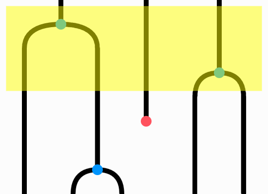
(a) The source of an interchanger.

(b) The source of an inverse associator (Definition 2.34).

Figure 2: Examples of rectangular subregions.

In order to define 1-cells, we introduced ordered string diagrams and then stipulated that ordered planar isotopic ordered string diagrams represented the same 1-cell. Likewise, in order to define 2-cells we introduce movies and identify these up to a certain equivalence relation.

Definition 2.10 (Movie).

Let $D_{1},\dots,D_{n}$ be 1-cells in the free Gray monoid on the computad $(C_{0},C_{1},C_{2},C_{3})$. A movie $D_{1}\to D_{n}$ is a sequence

$$D_{1}\overset{\gamma_{1,2}}{\Rightarrow}D_{2}\overset{\gamma_{2,3}}{\Rightarrow}\dots\overset{\gamma_{n-1,n}}{\Rightarrow}D_{n},$$

where $D_{i}$ are 1-cells and $\gamma_{i,i+1}$ are generating 2-cells such that $D_{i}$ and $D_{i+1}$ differ only by the application of $\gamma_{i,i+1}$ to a rectangular subregion.

As the 1-cells are represented by ordered string diagrams, if we draw these we get a series of transitions of planar diagrams. This is the reason for the name ‘movie’; each ordered string diagram is a frame of the movie. We call a contiguous subsequence of frames in a movie a clip.

We now introduce the following structural equalities by which movies will be identified.

Definition 2.11 (Structural equalities of a Gray monoid).

1. Type I rewrites. If two generating 2-cells occur consecutively in the movie, and the sets of generating 1-cells involved in each have zero intersection, their order may be interchanged.

   For example, take the movie generated from the pseudomonoid computad $\mathcal{P}$ (Definition 2.34), in which two associators are applied to four left-bracketed multiplication 1-cells, the first on the bottom pair and the second on the top pair. There is a Type I rewrite that switches this movie for an equal one where the associator is applied to the top pair of nodes first, then to the bottom pair.

   [ $\Rightarrow$ $\Rightarrow$ ] $=$ [ $\Rightarrow$ $\Rightarrow$ ]

2. Type II rewrites. These rewrites state that the downwards interchanger is the inverse of the upwards interchanger. If a 1-cell is unconnected to the 1-cell directly above it, we may insert an interchanger and its inverse into the movie; likewise, we may remove an interchanger and its inverse when they occur together.

   Here is an example generated from $\mathcal{P}$, where an interchanger between a unit and a multiplication node may be inserted:

   [ ] $=$ [ $\Rightarrow$ $\Rightarrow$ ]

3. Type III rewrites. When one 1-cell interchanges with another 1-cell, and either 1-cell is immediately acted upon by the following 2-cell, the movie may be rewritten so that the 2-cell occurs before the interchanger.

   The following example is generated by $\mathcal{P}$. Here a unit interchanges with a 1-cell after application of an associator; this may be rewritten to a movie where the associator occurs before the interchanger:

   [ $\Rightarrow$ $\Rightarrow$ $\Rightarrow$ ] $=$ [ $\Rightarrow$ $\Rightarrow$ $\Rightarrow$ ]

Remark 2.12.

The above equalities correspond to those in [Day1997, Definition 1]. In particular, the Type I rewrites correspond to naturality in the strict 2-category; the Type II rewrites correspond to the fact that the interchanger is an isomorphism; and the Type III rewrites correspond to equality (iii) in Day and Street’s definition.

Definition 2.13 (2-cells of a Gray monoid).

A 2-cell generated from $(C_{0},C_{1},C_{2})$ is a movie constructed from $(C_{0},C_{1},C_{2})$, where movies are identified up to the structural equalities of Definition 2.11.

Finally, the computad contains a set $E$ of specified equalities of 2-cells; for each element of this set there is a pair of $2$-cells (Definition 2.13) which are defined to be equal. In order to apply 2-cells to subregions of 1-cells, we introduced the notion of a rectangular subregion. Now, in order to apply rewrites to subregions of 2-cells, we introduce a higher-dimensional notion.

Definition 2.14.

Let $M=D_{1}\Rightarrow\dots\Rightarrow D_{n}$ be a 2-cell. A cuboidal subregion of $M$ is a choice of clip $c=D_{i_{1}}\Rightarrow\dots\Rightarrow D_{i_{2}}$, $1\leq i_{1}\leq i_{2}\leq n$, together with a fixed rectangular subregion $R$ of $D_{i_{1}}$, such that every transition in the clip acts on a rectangular subregion within $R$. A cuboidal subregion specifies a ‘sub-2-cell’ with source 1-cell $D_{i_{1}}|_{R}$ and target 1-cell $D_{i_{2}}|_{R}$ in the obvious way.

Definition 2.15 (Movie rewrites on cuboidal subregions).

Let $M$ be a movie. Whenever a cuboidal subregion of $M$ specifies a sub-2-cell related to another by an equality in $E$, $M$ is equal to the movie $M^{\prime}$ which is identical except for the replacement of the clip in the cuboidal subregion by the equal clip.

Definition 2.16 (2-cells following quotient by $E$).

The 2-cells generated from $(C_{0},C_{1},C_{2},E)$ are precisely movies constructed from $(C_{0},C_{1},C_{2})$, identified up to the structural equalities of Definition 2.11 and the specified equalities in the computad.

Now we have completely defined the 0-, 1- and 2-cells generated by the computad $\mathcal{C}$; all that remains is to define composition, and we have a full definition of our semistrict monoidal bicategory $G(\mathcal{C})$.

Definition 2.17 (Compositional structure of Gray monoid).

The 0-, 1- and 2-cell of a Gray monoid compose as shown in Table 3.

Note that the only thing that prevents this from being a strict monoidal bicategory is the failure of the interchange law. This weakness is sufficient for semistrictness.

Composition of 1-morphisms $(\forall f,g$ s.t. $s(g)=t(f))$	$:=$
Horizontal composition of 2-morphisms	$:=$
Vertical composition of 2-morphisms $(\forall f,g$ s.t. $s(g)=t(f))$
Monoidal product of objects	Concatenation of lists
Monoidal product of 1-morphisms	$:=$
Monoidal product of 2-morphisms

Table 3: The compositional structure of a Gray monoid.

We finish this section by defining some vocabulary.

Definition 2.18 (Isomorphism).

We make signatures of computads more concise by saying that a particular 2-cell $\mu$ is an isomorphism. This means that there is another 2-cell $\mu^{-1}$ in the signature with $s(\mu^{-1})=t(\mu)$ and $t(\mu^{-1})=s(\mu)$, satisfying $\mu\circ_{H}\mu^{-1}=id_{t(\mu)}$ and $\mu^{-1}\circ_{H}\mu=id_{s(\mu)}$.

Example 2.19.

In the pseudomonoid signature $\mathcal{P}$ of Definition 2.34, by specifying $\alpha$ as an isomorphism we avoid having to specify the 2-cell $\alpha^{-1}$ and two equalities.

Definition 2.20.

We call a movie whose source and target are equal a loop. We call a sequence of rewrites which take this movie to the trivial movie a contraction of the loop.

Definition 2.21.

When all the 2-cells featuring in an equality are isomorphisms, an equality still holds if the direction of all 2-cells on both sides of the equality is reversed. We call this the flip of the equality.

2.3 Braided and symmetric Gray monoids

The 0-, 1- and 2-cells of semistrict braided and symmetric monoidal bicategories (braided and symmetric Gray monoids) are generated and composed in exactly the same way as for naked Gray monoids. The difference is that the computads for braided and symmetric Gray monoids include additional structural generating cells which are not specified explicitly in the computad, but are rather constructed from the other specified data.

2.3.1 Braided Gray monoids

Definition 2.22.

A braided Gray monoid has the following additional structural generating cells and equalities.

• Additional generating 1-cells:

  • For every pair of 0-cells $A,B$, an ‘overbraiding’ 1-cell $R^{+}_{A,B}:A\otimes B\to B\otimes A$ and an ‘underbraiding’ 1-cell $R^{-}_{A,B}:A\otimes B\to B\otimes A$ . We depict these 1-cells as braidings in the 1-morphism diagram:

    $R^{+}_{A,B}=$

    $\sim\quad R^{-}_{A,B}=$

    The hexagonators are trivial; that is, for all 0-cells $A,B,C$ in $G(\Sigma)$, we have:

    $$R^{\pm}_{A\otimes B,C} =(id_{B}\otimes R^{\pm}_{A,C})\circ(R^{\pm}_{A,B}\otimes id_{C})$$

    $$R^{\pm}_{A,B\otimes C} =(R^{\pm}_{A,C}\otimes id_{B})\circ(id_{A}\otimes R^{\pm}_{B,C})$$

• Additional generating 2-cells:

  • ‘Braiding inverse-insert’ 2-isomorphisms $i^{+}_{AB},i^{-}_{AB}$ for each pair, $A,B$ of $0$-cells:

    $\overset{i^{+}_{AB}}{\Rightarrow}$

    $\overset{i^{-}_{AB}}{\Rightarrow}$

    These isomorphisms are strictly monoidal; that is, on products they are equal to the composites defined in the obvious way. For example:

    [ $\overset{i_{A,B\otimes C}^{+}}{\Rightarrow}$ ] = [ $\overset{i_{A,B}^{+}}{\Rightarrow}$ $\overset{i_{B,C}^{+}}{\Rightarrow}$ ]

  • ‘Pull-over’ and ‘pull-under’ 2-isomorphisms $PO_{f,B}$, $PO_{A,g}$, $PU_{f,B}$ and $PU_{A,g}$ for all $1$-cells $f:A\to C$, $g:B\to D$ in $\mathcal{C}$.

    $\overset{PO_{f,B}}{\Rightarrow}$

    $\overset{PU_{A,g}}{\Rightarrow}$

• Additional equalities:

  • $(\rightarrow\otimes\rightarrow)$. For $f:A\to C$, $g:B\to D$, we have the following equality:

    [ $\overset{PU_{C,g}}{\Rightarrow}$ $\overset{PO_{f,B}}{\Rightarrow}$ $\overset{\iota}{\Rightarrow}$ ] $=$[ $\overset{\iota}{\Rightarrow}$ $\overset{PO_{f,C}}{\Rightarrow}$ $\overset{PU_{A,g}}{\Rightarrow}$ ]

  • $(\cdot\;\otimes\Downarrow)$. For morphisms $f,g:B\to D$ and a 2-morphism $\alpha:f\to g$, we have the following equality. (Here and elsewhere, we use highlighting to make clear where a 2-morphism is about to be applied.)

    [ $=$ $\overset{\alpha}{\Rightarrow}$ $\overset{PU_{A,g}}{\Rightarrow}$ ] $=$ [ $\overset{PU_{A,f}}{\Rightarrow}$ $=$ $\overset{\alpha}{\Rightarrow}$ ]

  • $(\Downarrow\otimes\;\cdot)$. As above, but for $f,g:A\to C$ and with a pull-over.

  • $(\rightarrow\rightarrow\otimes\;\cdot)$. We have the following equality for morphisms $f:A\to C,g:C\to E$, where the composition $c$ is a strict equality since we are in a Gray monoid.

    [ $\overset{PO_{g,A}}{\Rightarrow}$ $\overset{PO_{f,A}}{\Rightarrow}$ $=$ $\overset{c}{=}$ ]

    $=$ [ $=$ $\overset{c}{=}$ $\overset{PO_{g\circ f,A}}{\Rightarrow}$ ]

  • $(\cdot\;\otimes\rightarrow\rightarrow)$. As above, but with $f:B\to D,g:D\to F$ and pull-unders.

  • PT-B. For any 1-morphism $g:B\to D$, the following 2-morphisms are equal:

    [ $\overset{i^{+}_{AD}}{\Rightarrow}$ $\overset{PU_{A,g}}{\Rightarrow}$ ] $=$ [ $\overset{i^{+}_{AB}}{\Rightarrow}$ $\overset{PU^{-1}_{g,A}}{\Rightarrow}$ ]

    Similar equations hold where $i^{+}_{A,B}$ is changed for $i^{-}_{A,B}$, and/or the 1-cell pulled through is $f:A\to C$ rather than $g:B\to D$.

  • ADJ. $i^{+}_{A,B}$ and $i^{-}_{A,B}$ are the units of adjoint equivalences.

  • $S^{+}=S^{-}$. The two possible instantiations of the braid move $\sigma_{i}\sigma_{i+1}\sigma_{i}\to\sigma_{i+1}\sigma_{i}\sigma_{i+1}$ are equal.

The axioms we have specified are those of a twice-degenerate semistrict 4-category in the definition of Bar and Vicary [Bar2017] and are slightly stricter than in any previous definition of a braided Gray monoid  [Kapranov1994, Baez1996, Crans1998, Gurski2011]. The two points of difference with the strictest previous definition [Crans1998] are the following.

• The ‘hexagonators’ in the Bar-Vicary definition are trivial; this corresponds to strictness of composition in the semistrict 4-category. The strict monoidality of the braiding inverse-insert 2-cells follows from this.

• There is an extra axiom in the Bar-Vicary definition, PT-B, which relates a braiding inverse-insert and pullthrough above to a braiding inverse-insert and pullthrough below. This axiom follows from Homotopy Generator VI in the definition of Bar and Vicary.

The Crans definition with trivial hexagonators remains semistrict.

Theorem 2.23 (Semistrictness with trivial hexagonators).

For any computadic Crans braided monoidal bicategory, the quotient homomorphism $\phi$ which identifies all braiding 1-cells with the corresponding ‘expanded’ composite of braidings of generating 1-cells (- ‣ • ‣ 2.22), and sends all hexagonators to the identity, is a braided monoidal biequivalence.

Proof.

See Appendix LABEL:app:semistrictnesshexagonators. ∎

Having resolved the issue of the trivial hexagonators, we turn to the PT-B equality. It seems that this equality, which is topologically well-motivated, is not implied by the other equalities. The arguments for the correctness of Bar and Vicary’s definition support it; indeed, the proof that every equivalence in a semistrict 4-category can be promoted to an adjoint equivalence satisfying the butterfly equations depends on Homotopy Generator VI [Bar2017]. It is also an essential ingredient in our algorithm for putting 1-cells in TSNF (Theorem 2.32).

PT-B may have been omitted previously because previous authors worked only with braided monoidal bicategories with no generating 1-cells. In that case, PT-B follows straightforwardly from ADJ, rendering a separate axiom unnecessary. In the symmetric setting, PT-B is implied by stronger coherence results.

2.3.2 Symmetric Gray monoids

The axioms we have chosen for symmetric Gray monoids are somewhat weaker than those of the quasistrict definition of Schommer-Pries [Schommer-Pries2009]. The primary advantage of using a weaker definition is that our proofs of fullness and functoriality of the biequivalences we define apply equally to non-braided, braided and symmetric Gray monoids.

Definition 2.24.

A symmetric Gray monoid is a braided Gray monoid with the following additional structural generating cells and equalities.

• Additional generating 2-cells:

  • A ‘syllepsis’ 2-isomorphism $\sigma_{AB}$ for all 0-cells $A,B$, which controls the symmetry of the braiding:

    $\overset{\sigma_{AB}}{\Rightarrow}$

    As with the braiding inverse-insert, the syllepsis on monoidal products is the composite of the syllepses on the factors.

• Additional equalities of 2-cells:

  • PT-SYL. For every 0-cell $A$ and 1-cell $g:B\to D$, the following equality:

    [ $\overset{\sigma_{AD}}{\Rightarrow}$] $=$ [ $\overset{PU_{A,g}}{\Rightarrow}$ $\overset{PO_{g,B}}{\Rightarrow}$$\overset{\sigma_{AB}}{\Rightarrow}$]

    The equality PT-SYL${}_{f,B}$ is defined similarly for all 0-cells $B$ and 1-cells $f:A\to C$.

  • SYM. The following 2-morphisms are equal:

    [ $=$ $\overset{\sigma_{B,A}}{\Rightarrow}$] $=$ [ $=$ $\overset{\sigma_{A,B}}{\Rightarrow}$]

Here, rather than take the braiding inverse-inserts and syllepses to be identities, as in the quasistrict definition of Schommer-Pries, we only require PT-B, which follows from triviality of the braiding inverse-inserts in the quasistrict definition; and PT-SYL, another axiom similar to PT-B but involving the syllepsis, which follows from triviality of the syllepsis in the quasistrict definition. The semistrictness of this definition of symmetric Gray monoids is therefore implied by the semistrictness of Schommer-Pries’ quasistrict definition [Schommer-Pries2009, Theorem 2.96].

Definition 2.25.

Every computad for a naked Gray monoid can also be taken as a computad for a braided or a symmetric Gray monoid; likewise, every computad for a braided Gray monoid can also be taken as a computad for a symmetric Gray monoid.

2.4 Coherence for braided and symmetric Gray monoids

In this section we treat coherence results for braided and symmetric Gray monoids which will be used in the proof of our main theorem. We first recall two important results about braided and symmetric Gray monoids; here we only state the computadic versions, although they hold in greater generality.

Theorem 2.26 ([Gurski2011, Theorem 25]).

Let $C$ be a braided Gray monoid computad with no non-structural generating 2-cells, whose non-structural generating 1-cells all have exactly one 0-cell as source and one 0-cell as target. In the braided Gray monoid generated from $C$, all parallel 2-cells are equal, and two structural 1-cells are isomorphic iff they have the same underlying element of the braid group.

Theorem 2.27 ([Gurski2013, Theorem 1.23]).

Let $C$ be a symmetric Gray monoid computad with no non-structural generating 2-cells, whose non-structural generating 1-cells all have exactly one 0-cell as source and one 0-cell as target. In the symmetric Gray monoid generated from $C$, all parallel 2-cells are equal, and two structural 1-cells are isomorphic iff they have the same underlying permutation.

We now introduce a useful normal form for 1-cells in braided and symmetric Gray monoids.

Definition 2.28 (Output string).

Consider a 1-cell diagram in a braided Gray monoid. For any generating 1-cell $N$ in the diagram with a single generating 0-cell in its output, we define its output string to be the string extending from $N$ to the next non-structural 1-cell to which the string is input; or to the roof of the diagram if it is not input to another non-structural 1-cell.

Let $N$ be a non-structural generating 1-cell in some frame of a movie. Provided that no non-structural 2-cells occur on rectangular subregions containing $N$, it is always possible to identify $N$ in previous and subsequent frames, where it may have been moved by interchangers and pullthroughs. We may therefore speak about $N$ as being in a clip, rather than just in a frame.

Definition 2.29 (TSNF).

Let $M$ be a clip in a computadic braided Gray monoid, containing some non-structural generating 1-cell $N$ whose output is a single generating 0-cell. We say that $N$ is in top string normal form (TSNF) in $M$ if no generating 2-cells act on rectangular subregions containing the output string of $N$ during $M$.

Example 2.30.

In the clip below the output string of the lowest generating 1-cell is highlighted. The lowest generating 1-cell is not in TSNF because a braiding cancellation, a braiding inverse-insert, and then a pullthrough occur on the output string during the clip.

[ $\Rightarrow$ $\Rightarrow$ $\Rightarrow$]

As we will now show, we can always put a generating 1-cell in TSNF, provided that no non-structural 2-cells occur on a rectangular subregion containing some part of the output string. First we define a useful movie rewriting technique.

Definition 2.31 (Insert IPI).

Let $N$ be a 1-cell in a clip in a braided or symmetric Gray monoid. We can rewrite the clip by using Type II rewrites and invertibility of the pullthroughs to move $N$ up or down the frame. We say that we ‘insert IPI’. For example, here we insert IPI to move the lowest generating 1-cell to the top of the frame and back to the bottom again:

[ ] $=$ [ $\Rightarrow$ $\Rightarrow$ ] $=$ [ $\Rightarrow$ $\Rightarrow$ $\Rightarrow$ $\Rightarrow$ ]

Now we state the main results of this section. We postpone their proofs to Appendix LABEL:sec:proofsforgraymoncohappendix.

Theorem 2.32 (Putting a 1-cell in TSNF).

Let $M$ be a clip in a computadic braided Gray monoid. Let $N$ be a non-structural generating 1-cell whose output is a single generating 0-cell. If no non-structural 2-cells occur on a rectangular subregion containing the output string of $N$ during $M$, then there exists a series of rewrites to put $N$ in TSNF.

Theorem 2.33 (Extended coherence for computadic braided and symmetric Gray monoids).

Let $C$ be a computad for a braided or symmetric Gray monoid with no nonstructural generating 2-cells, whose generating 1-cells all have a single generating 0-cell as output. Then all parallel 2-cells in the braided or symmetric Gray monoid generated from $C$ are equal.

2.5 Computads for braided and symmetric pseudomonoids

The following computads follow the definitions of Day and Street [Day1997].

Definition 2.34.

The pseudomonoid computad $\mathcal{P}$ is the naked Gray monoid computad defined as follows.

• 0-cells: $\{C\}$.

• 1-cells: $m:C\otimes C\to C$ and $u:I\to C$.

  $m=$

  $u=$

• 2-cells: $\alpha$ (associator), $\lambda$ (left unitor) and $\rho$ (right unitor), all isomorphisms (Definition 2.18).

  $\overset{\alpha}{\Rightarrow}$

  $\overset{\lambda}{\Rightarrow}$

  $\overset{\rho}{\Rightarrow}$

  We will occasionally call the unitors $\lambda,\rho$ unit destruction operators and the inverse unitors $\lambda^{-1},\rho^{-1}$ unit creation operators.

• Equalities:

  • Pentagon:

    [ $\overset{\alpha}{\Rightarrow}$ $\overset{\iota}{\Rightarrow}$ $\overset{\alpha}{\Rightarrow}$ ] $=$ [ $\overset{\alpha}{\Rightarrow}$ $\overset{\alpha}{\Rightarrow}$ $\overset{\alpha}{\Rightarrow}$ ]

  • Triangle:

    [ $\overset{\alpha}{\Rightarrow}$ $\overset{\lambda}{\Rightarrow}$ ] $=$ [ $\overset{\rho}{\Rightarrow}$ ]

Definition 2.35.

The braided pseudomonoid computad $\mathcal{P}^{\text{br}}$ is the braided Gray monoid computad with all the generating cells of $\mathcal{P}$, and the following additional data.

• 2-cells: An isomorphism $c$ (the commutator):

  

  $\overset{c}{\Rightarrow}$

• Equalities:

  • Hexagon 1:

    [ $\overset{c}{\Rightarrow}$ $\overset{\alpha^{-1}}{\Rightarrow}$ $\overset{c}{\Rightarrow}$ ] $=$ [ $\overset{\alpha^{-1}}{\Rightarrow}$ $\overset{PU^{-1}_{C,m}}{\Rightarrow}$ $\overset{c}{\Rightarrow}$ $\overset{\alpha^{-1}}{\Rightarrow}$ ]

  • Hexagon 2:

    [ $\overset{\alpha}{\Rightarrow}$ $\overset{PO^{-1}_{m,C}}{\Rightarrow}$ $\overset{c}{\Rightarrow}$ $\overset{\alpha}{\Rightarrow}$ ] $=$ [ $\overset{c}{\Rightarrow}$ $\overset{\alpha}{\Rightarrow}$ $\overset{c}{\Rightarrow}$ ]

Definition 2.36.

The symmetric pseudomonoid computad $\mathcal{P}^{\text{sym}}$ is the symmetric Gray monoid computad with all the generating cells of $\mathcal{P}^{\text{br}}$, and the following additional data.

• Equalities:

  • Symmetry:

    [ ] = [ $\overset{\sigma^{-1}}{\Rightarrow}$ $\overset{c}{\Rightarrow}$ $\overset{c}{\Rightarrow}$]

2.6 Theories of monoids

Before concluding the background section, we review the theory of PROs, PROBs and PROPs for monoids and commutative monoids which was summarised in Table 1 of the introduction.

Definition 2.37.

The monoid computad ${\bf M}$ is generating data for a PRO, derived from the pseudomonoid computad by considering the generating 2-cells as equalities of 1-cells and forgetting equalities of 2-cells.

Definition 2.38.

The commutative monoid computad ${\bf CM}$ is generating data for a PROB, derived from the pseudomonoid computad by considering the generating 2-cells as equalities of 1-cells and forgetting equalities of 2-cells.

We define a combinatorial category isomorphic to the PRO for monoids.

Definition 2.39.

The objects of ${\bf\Delta}$ are natural numbers $\underline{n}\in\mathbb{N}$, and its 1-cells $\underline{m}\to\underline{n}$ are monotone functions $\{1,\dots,m\}\to\{1,\dots,n\}$ (i.e. functions satisfying $f(i)<f(j)\;\,\forall\,i<j$). Composition is composition of functions, and monoidal product is the coproduct in ${\bf Set}$.

In order to identify 1-cells in the PRO for monoids with monotone functions, one considers connectedness between inputs and outputs of a 1-cell. In the absence of a braiding, this must correspond to a monotone function. An output which is not connected to any input must come from a unit. An example is shown in Figure 3. The following proposition makes this precise.

Proposition 2.40.

The PRO on the monoid computad, FM, is isomorphic to ${\bf\Delta}$.

Proof.

We define a functor ${\bf\Delta}\to{\bf FM}$.

• On 0-cells: The objects of both categories are natural numbers; let the map on 0-cells be the identity function.

• On 1-cells: Given a function $f:\underline{m}\to\underline{n}$, we define a morphism $\tilde{f}$ in FM as follows. Let $\mu:\underline{2}\to\underline{1}$ be the multiplication 1-cell in ${\bf FM}$, and $u:\underline{0}\to\underline{1}$ be the unit. Let $p_{i}=|f^{-1}(i)|$ be the cardinality of the preimage of $i\in\{1,\dots,n\}$. Let $\mu^{n}:\underline{n}\to\underline{1}$ be the composition of $n-1$ multiplications, left bracketed; for example, $\mu^{4}=\mu\circ(\mu\otimes\text{Id})\circ(\mu\otimes\text{Id}\otimes\text{Id})$. We set $\mu^{1}=\text{Id}$ and $\mu^{0}=u$. Then we define

  $$\tilde{f}=(\mu^{p_{1}}\otimes\cdots\otimes\mu^{p_{n}}).$$ (1)

It is easy to check that this is an isomorphism of categories [Davydov2010, Section 2.1].

Figure 3: The image of the function $f:\underline{5}\to\underline{3}$, $f(1)=f(2)=f(3)=1$, $f(4)=f(5)=3$ under the isomorphism ${\bf\Delta}\to{\bf FM}$.

∎

Definition 2.41.

We call the compositions $\mu^{n}$ multiplication trees, or just trees.

We now consider the free braided monoidal category (PROB) ${\bf F^{br}M}$ on the monoid computad. We can always pull the monoid structure through any braidings, which allows us to split any 1-cell into a braid followed by a monoid map. The 1-cells of the isomorphic combinatorial category will therefore have a braid part and a monotone function part. ‘Pulling through’ is formally a distributive law [Day2003] between the braid structure and the monoid structure, which may be used to define composition. The following lemma and proposition make this precise.

We write the image of the embedding ${\bf\Delta}\hookrightarrow{\bf F^{br}M}$, which picks out the morphisms without braiding, as ${\bf\Delta}\subset{\bf F^{br}M}$. Let ${\bf B}$ be the free braided monoidal category on a single object; we write the image of the embedding ${\bf B}\hookrightarrow{\bf F^{br}M}$, which picks out the morphisms made entirely of braids, as ${\bf B}\subset{\bf F^{br}M}$.

Lemma 2.42 ([Day2003, Section 4]).

For any $b\in{\bf B}$, $f\in{\bf\Delta}$, there exist unique morphisms $b^{\prime}\in{\bf B}$, $f^{\prime}\in{\bf\Delta}$ such that $b\circ f=f^{\prime}\circ b^{\prime}$ in ${\bf F^{br}M}$; there is a corresponding distributive law

$$B_{n}\times{\bf\Delta}(m,n)\overset{\delta_{m,n}}{\to}{\bf\Delta}(m,n)\times B_{m}$$ (2)

where $B_{n}$ is the braid group on $n$ points and ${\bf\Delta}(m,n)$ are the morphisms $\underline{m}\to\underline{n}$ in ${\bf\Delta}$.

Under the distributive law, let $\delta_{m,n}^{B}:=\pi_{B_{m}}\circ\delta(m,n)$ be the braid part of the image, and let $\delta_{m,n}^{\Delta}:=\pi_{\Delta}\circ\delta(m,n)$ be the monoid part.

Definition 2.43.

The braided monoidal category ${\bf B\Delta}$ has objects natural numbers. Morphisms $\underline{m}\to\underline{n}$ are pairs $(\sigma,f)$, where $\sigma\in B_{m}$ and $f\in{\bf\Delta}(m,n)$. Composition is defined using the distributive law and composition in ${\bf\Delta}$ and the braid group in the following way. For $(\sigma_{1},f_{1})\in\mathrm{Hom}(\underline{m},\underline{n})$ and $(\sigma_{2},f_{2})\in\mathrm{Hom}(\underline{n},\underline{o})$, we define:

$$(\sigma_{2},f_{2})\circ(\sigma_{1},f_{1}):=(\delta^{B}_{m,n}(\sigma_{2},f_{1})\circ\sigma_{1},f_{2}\circ\delta^{\Delta}_{m,n}(\sigma_{2},f_{1})).$$ (3)

The monoidal product on objects is addition of natural numbers; on morphisms, for $(\sigma_{1},f_{1})\in\mathrm{Hom}(\underline{m},\underline{m^{\prime}})$, $(\sigma_{2},f_{2})\in\mathrm{Hom}(\underline{n},\underline{n^{\prime}})$ we define

$$(\sigma_{1},f_{1})\otimes(\sigma_{2},f_{2}):=(\sigma_{1}\times\sigma_{2},f_{1}\sqcup f_{2})\in\mathrm{Hom}(\underline{m}+\underline{n},\underline{m^{\prime}}+\underline{n^{\prime}}),$$ (4)

where $\sqcup$ is the coproduct in ${\bf Set}$ and $\times$ is the Cartesian product of groups. The braiding $\sigma_{m,n}:\underline{m}\otimes\underline{n}\to\underline{n}\otimes\underline{m}$ is simply the corresponding braid $(\sigma,\mathrm{id}_{\underline{m+n}})\in\mathrm{Hom}(\underline{m+n},\underline{m+n})$.

Proposition 2.44.

The PROB on the monoid computad, ${\bf F^{br}M}$, is isomorphic to ${\bf B\Delta}$.

Proof.

See [Day2003, Section 4]. The isomorphism is the identity function on 0-cells; on 1-cells, it is simply $(\sigma,f)\mapsto\tilde{f}\circ\sigma$, where $\tilde{f}$ is defined as in (1). The diagrammatic representation is shown in Figure 4.

$(\sigma,f)\;\mapsto\;\;$

Figure 4: The image of the pair of a braiding and a monotone function under the isomorphisms defined in this section.

∎

The PROP for monoids, ${\bf F^{sym}M}$, can be treated similarly. Let $S_{n}$ be the symmetric group on $n$ points. There is a surjective homomorphism $q:B_{n}\to S_{n}$, which takes a braid to its underlying permutation, and is suitably compatible with the distributive law. We therefore obtain another distributive law

$$S_{n}\times{\bf\Delta}(m,n)\overset{\delta^{s}_{m,n}}{\to}{\bf\Delta}(m,n)\times S_{m}$$

encoding the effect of pulling the monoid structure through the permutations.

Definition 2.45.

The symmetric monoidal category ${\bf S\Delta}$ has natural numbers for objects. Morphisms $\underline{m}\to\underline{n}$ are pairs of a morphism in ${\bf\Delta}(m,n)$ and an element of $S_{m}$. Composition, monoidal product and braiding are defined as for ${\bf B\Delta}$ (3-4), using the distributive law $\delta^{s}$.

Proposition 2.46.

The PROP on the monoid computad, ${\bf F^{sym}M}$, is isomorphic to ${\bf S\Delta}$.

Proof.

See [Day2003, Section 4]. Again, the isomorphism is the identity function on 0-cells, and on 1-cells it is $(s,f)\mapsto\tilde{f}\circ s$, as in Figure 4. ∎

We now turn to commutative monoids. One needs a braiding in order to define the commutativity equality, so it is meaningless to consider the PRO in this case.

We begin with the PROB ${\bf F^{br}CM}$. Since all the equations in the monoid computad are satisfied, ${\bf F^{br}CM}$ will be a quotient category of ${\bf F^{br}M}$. The quotient is defined as follows. Given some morphism $(\sigma,f)$, the commutativity axiom allows us to alter $\sigma$ by absorbing or emitting braidings from the trees of $f$. For example, Figure 5 shows emission of the braiding $\sigma_{2}^{-1}\in B_{3}$ from a single tree with 3 inputs.

Figure 5: Emission of the braiding $\sigma_{2}^{-1}\in B_{3}$ from a single tree with 3 inputs. The first equality uses associativity and the braided structure of the category, and the second uses commutativity.

Each $f\in{\bf\Delta}(m,n)$ has fibres $f^{-1}(i)$, $i\in\{1,\dots,n\}$; we write $p_{i}=|f^{-1}(i)|$. Using the commutativity equality, we can create braidings or inverse braidings underneath the trees, move them downwards and absorb them into $\sigma$. Letting $p_{i}=|f^{-1}(i)|$, we obtain an action of $\prod_{i=1}^{n}B_{p_{i}}$ on $B_{m}$ by postcomposition. Figure 6 depicts this for one morphism $\underline{7}\to\underline{3}$.

Figure 6:

Let $\sim_{f}$ be the equivalence relation which identifies elements of $B_{n}$ if they are in the same orbit under this action. The distributive law is suitably compatible with the action, which allows us to define the following category.

Definition 2.47.

The category ${\bf B\Delta/\sim}$ is defined in the same way as ${\bf B\Delta}$, but where the morphisms $f:\underline{m}\to\underline{n}$ are now pairs $(\bar{\sigma},f)$, where $f\in\Delta(m,n)$ and $\bar{\sigma}\in B_{m}/\sim_{f}$.

Proposition 2.48.

The PROB on the commutative monoid computad is isomorphic to ${\bf B\Delta/\sim}$.

Proof.

See [Lavers1997, Theorem 2]. Again, the isomorphism takes $(\bar{\sigma},f)\mapsto\tilde{f}\circ\bar{\sigma}$, as in Figure 4. ∎

Finally, we consider the PROP ${\bf F^{sym}CM}$. Again, this will be a quotient of ${\bf F^{sym}M}$. Rather than braidings, we now emit permutations from the trees, giving rise to an action of $\prod_{i=1}^{n}S_{p_{i}}$ on $S_{m}$ by postcomposition, which induces a quotient $S_{m}/\sim_{f}$. As before, we define the following category.

Definition 2.49.

The category ${\bf S\Delta/\sim}$ is defined in the same way as ${\bf S\Delta}$, but where the morphisms $f:\underline{m}\to\underline{n}$ are now pairs $(\bar{\sigma},f)$ of $f\in\Delta(m,n)$ and $\bar{\sigma}\in S_{m}/\sim_{f}$.

It turns out that ${\bf S\Delta/\sim}$ is isomorphic to a familiar category.

Definition 2.50.

The category ${\bf FS}$ has objects natural numbers, and morphisms $\underline{m}\to\underline{n}$ functions $\{1,\dots,m\}\to\{1,\dots,n\}$, where $\underline{0}$ is the empty set.

Proposition 2.51.

The PROP ${\bf F^{sym}CM}$ on the commutative monoid computad, the category ${\bf S\Delta/\sim}$, and ${\bf FS}$ are all isomorphic.

Proof.

[Davydov2010, Proposition 2.3.3]. The isomorphism between ${\bf F^{sym}CM}$ and ${\bf S\Delta/\sim}$ is as in Proposition 2.48. For clarity, we define explicitly the isomorphism ${\bf FS}\to{\bf F^{sym}CM}$. Again, the morphisms in the image are of the form $\tilde{f}\circ\bar{\sigma}$ shown in Figure 4; we need only define $\bar{\sigma}_{f}\in S_{n}/\sim_{f}$ and $\tilde{f}\in{\bf\Delta}(m,n)$ for a given function $f:\underline{m}\to\underline{n}$.

We define $\tilde{f}$ as before. Again, Let $\mu:\underline{2}\to\underline{1}$ be the multiplication in ${\bf F^{br}CM}$, and $u:\underline{0}\to\underline{1}$ be the unit. Again, let $p_{i}=|f^{-1}(i)|$ be the cardinality of the preimage of $i\in\{1,\dots,n\}$. Let $\mu^{n}:\underline{n}\to\underline{1}$ be the composition of $n-1$ multiplications, left bracketed; for example, $\mu^{4}=\mu\circ(\mu\otimes\text{Id})\circ(\mu\otimes\text{Id}\otimes\text{Id})$. Set $\mu^{1}=\text{Id}$ and $\mu^{0}=u$. Then

$$\tilde{f}:=(\mu^{p_{1}}\otimes\cdots\otimes\mu^{p_{n}}).$$

Now we define $\bar{\sigma}_{f}$. We write a permutation of $m$ elements as rearrangement of $1,\dots,m$; for example, the cycle $(1)(23)$ may be written as $\langle 132\rangle$. For $S\subset\mathbb{N}$, let $[S]$ be the set $S$ with elements written in ascending order. In this notation, we define

$$\sigma_{f}=\langle[f^{-1}(1)][f^{-1}(2)]\dots[f^{-1}(n)]\rangle.$$

Then $\bar{\sigma}_{f}$ is the equivalence class of this permutation under the quotient. ∎

The results of this section are summarised in Table  1.

3 Coherence for braided and symmetric pseudomonoids

In this section we state and prove our main results, which were summarised in Table 2.

3.1 Combinatorial bicategories

First we define the combinatorial bicategories that appear in the table.

Definition 3.1.

A locally discrete bicategory is one with only identity 2-cells.

Any category may be considered as a strict locally discrete bicategory by adding identity 2-cells; this preserves monoidality, braiding and symmetry. We therefore obtain the Gray monoid ${\bf\Delta}$, the braided Gray monoids ${\bf B\Delta}$ and ${\bf B\Delta/\sim}$, and the symmetric Gray monoids ${\bf S\Delta}$ and ${\bf FS}$.

We now define another combinatorial categorification of ${\bf FS}$, which will correspond to the theory of braided pseudomonoids in a symmetric monoidal bicategory. In this case, not all diagrams commute, so we need to add more 2-cells to ${\bf FS}$ than just identities.

Definition 3.2.

A locally totally disconnected 2-category is one whose 2-cells are all endomorphisms.

Definition 3.3.

${\bf FS}^{\text{br}}$ is a locally totally disconnected strict 2-category obtained from ${\bf FS}$ by adding 2-cells as follows.

For any 1-cell $f:\underline{m}\to\underline{n}$, we add a set of 2-cells $\mathrm{Hom}(f,f)=\prod_{i=1}^{n}PB_{p_{i}}$, where $p_{i}=|f(i)^{-1}|$ and $PB_{n}$ is the pure braid group on $n$ points. We define the following compositional structure on these 2-cells.

• Horizontal composition. For any $f:\underline{m}\to\underline{n}$, and $\sigma,\tau\in\mathrm{Hom}(f,f)$, we define $\tau\circ_{H}\sigma\in\mathrm{Hom}(f,f)$ to be the composition $\tau\circ\sigma\in\prod_{i=1}^{n}PB_{p_{i}}$.

• Vertical composition. For any $f:\underline{m}\to\underline{n}$, $g:\underline{n}\to\underline{o}$, and $\sigma_{m}\in\mathrm{Hom}(f,f)$, $\sigma_{n}\in\mathrm{Hom}(g,g)$, we define $\sigma_{n}\circ_{V}\sigma_{m}\in\mathrm{Hom}(g\circ f,g\circ f)$ as follows:

  $$\sigma_{n}\circ_{V}\sigma_{m}:=\sigma_{m}\delta_{m,n}^{B}(f_{\Delta},\sigma_{n}).$$

  Here $\delta^{B}_{m,n}$ is the braided part of the image of the distributive law (2) and $f_{\Delta}$ is the ${\bf\Delta}$-factor of $f$ in the decomposition ${\bf FS}={\bf S\Delta}$ of Proposition 2.51.

• Monoidal product. For any $f:\underline{m}\to\underline{n},g:\underline{o}\to\underline{p}$, and $\sigma_{m}\in\mathrm{Hom}(f,f)$, $\sigma_{n}\in\mathrm{Hom}(g,g)$, we define $\sigma_{m}\otimes\sigma_{n}:f\otimes g\to f\otimes g$ to be the Cartesian product of braids $(\sigma_{m},\sigma_{n})\in B_{m}\times B_{n}\subset B_{m+n}$.

It is straightforward to check that this defines a strict symmetric Gray monoid.

3.2 Biequivalences

Definition 3.4.

A (braided/symmetric) biequivalence of Gray monoids is a homomorphism of (braided/symmetric) Gray monoids [Day1997] which is essentially surjective on objects and 1-morphisms, and fully faithful on 2-morphisms.

We define the biequivalences of Table 2 by categorifying the isomorphisms of Section 2.6. Those isomorphisms map $(\sigma,f)$ to $\tilde{f}\circ\tilde{\sigma}$, where:

• $\sigma$ is an element of the braid group, the symmetric group or a quotient of those groups.

• $\tilde{\sigma}$ is the same element considered as a morphism in the free braided or symmetric monoidal category on a single object.

• $f$ is a monotone function.

• $\tilde{f}$ is the corresponding braid-free morphism in the PRO, PROB or PROP.

This definition needs to be adapted slightly for the higher setting. Firstly, in order to specify $\tilde{f}$, one must give the height of each generating 1-cell, since planar isotopy is now an isomorphism rather than an equality. Secondly, in order to specify $\tilde{\sigma}$, one must now specify a word in the generators of the Artin presentation of the braid group, rather than simply the isotopy class of braids, the permutation, or the equivalence class under the quotient, since the braid relations are now also isomorphisms. To resolve these issues, we make the following definitions. We first consider the braid-free part.

Definition 3.5.

Let ${\bf\Delta}$ be the subcategory of braid-free morphisms of any of the PROs, PROBs or PROPs for monoids or commutative monoids. We say that a diagram in ${\bf\Delta}$ is in standard form if the heights of the 1-cells in the trees rise from left to right, as in Figures 3 and 6.

We now consider the braid part.

Definition 3.6.

We define the representative word of a braid or permutation as follows.

• For $\sigma\in B_{n}$: Its representative word is its Artin normal form.

• For $\overline{\sigma}\in B_{n}/\sim_{f}:$ We use the Axiom of Choice to pick a coset representative for each $\overline{\sigma}\in B_{n}/\sim$, and say that the Artin normal form of this chosen representative is the representative word of $\overline{\sigma}$.

• For $s\in S_{n}$: We write the permutation as a braid diagram in the following way. We draw a straight line from each input to the output which is its image under the permutation. At crossings, we use the convention that the string connected to the leftmost input crosses on top. If there are any triple crossings then we pull the top string downwards in order to remove them. If two crossings occur at the same height, we deform the diagram so that the leftmost crossing occurs first. We may then read off a word in the braid generators from the diagram; we say that this is the representative word of $s$.

• For $\overline{s}\in S_{n}/\sim_{f}:$ We use the Axiom of Choice to pick a coset representative for each $\overline{s}\in S_{n}/\sim_{f}$, and obtain a representative word for this representative as for $s\in S_{n}$.

Using these definitions, it is straightforward to specify the biequivalences on 0- and 1-cells. We define them as maps from the combinatorial category to the higher PRO.

Definition 3.7 (Biequivalences on 0- and 1-cells).

Each biequivalence in Table 2 is defined on 0-cells and 1-cells as follows.

• On 0-cells the map takes $\underline{n}\in\mathbb{N}$ to $A^{\otimes n}$, where $A$ is the unique generating 0-cell of the higher PRO.

• On 1-cells, $(\sigma,f)$ is mapped to $\tilde{f}\circ\tilde{\sigma}$, where $\tilde{f}$ is in standard form and $\tilde{\sigma}$ is the braid defined by the representative word of $\sigma$.

Definition 3.8 (Biequivalences on 2-cells for locally discrete bicategories).

For the locally discrete categorifications, the biequivalences in Table 2 are defined on 2-cells by taking identity 2-cells to identity 2-cells.

Finally, we define the biequivalence on 2-cells for the only non-locally discrete categorification.

Definition 3.9.

The biequivalence from ${\bf FS^{\text{br}}}$ in Table 2 is defined on 2-cells as follows. Let $\sigma\in\mathrm{Hom}_{{\bf FS}^{\text{br}}}(f,f)=\prod_{i=1}^{n}PB_{p_{i}}$, and let $\sigma_{i}$ be the factors of $\sigma$ in the product. The 2-cell in the image of $\sigma$ is a movie defined as follows.

1. We use the symmetric structure of the category to create the braid $\sigma_{1}$ directly beneath the tree $m^{p_{1}}$, working from left to right. By Theorem 2.27 there is no ambiguity regarding the 2-morphism we use to do this.

2. We remove the braid using commutators and inverse commutators as follows. Recall that the tree is initially left bracketed.

   1. Use associators to bring the lowest 1-cell in the tree $m^{p_{i}}$ directly above the highest braid, using the following iterative method: Associate the bottom 1-cell to the right. If this is impossible associate the 1-cell above it to the right and return. If this is impossible associate the 1-cell above that to the right and return. Etc. Repeat until the lowest multiplication is directly above the braiding to be absorbed.

   2. Use a commutator or an inverse commutator to remove the braiding. A commutator removes a positive braiding; an inverse commutator removes a negative braiding by producing a positive braiding, then cancelling the two.

   3. Use the inverse of the original sequence of associators to left bracket the tree again.

   4. Repeat until $\sigma_{1}$ has been entirely removed by commutators.

   An example is shown in Figure 7.

3. Now create $\sigma_{2}$ beneath the tree $m^{p_{2}}$ and absorb. Repeat for all trees, working from left to right. This completes the loop.

A schematic is shown in Figure 8.

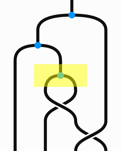
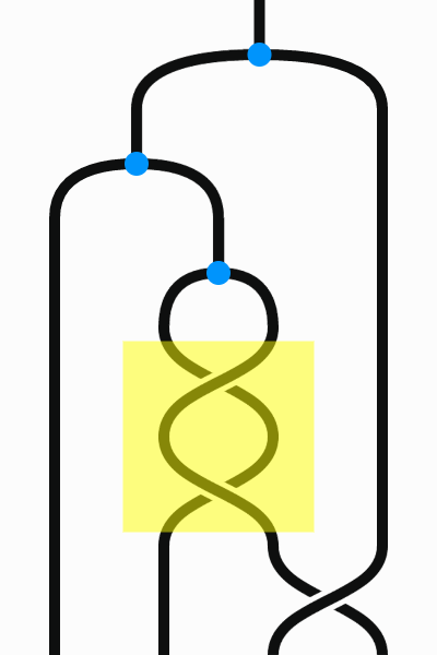
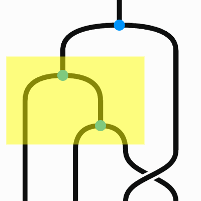
		$\Rightarrow$		$\Rightarrow$		$\Rightarrow$		$\Rightarrow$		$\Rightarrow$
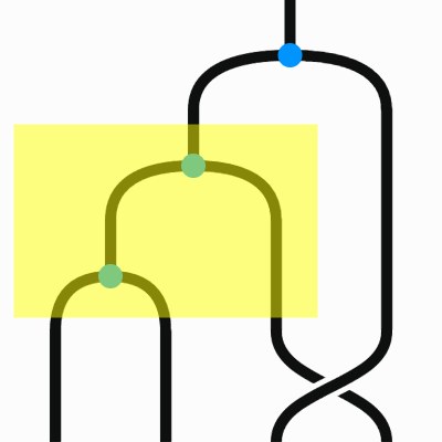
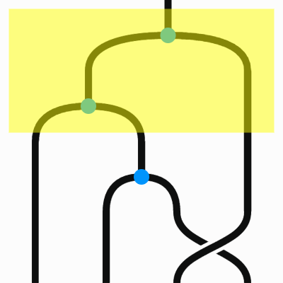
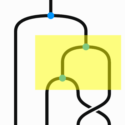
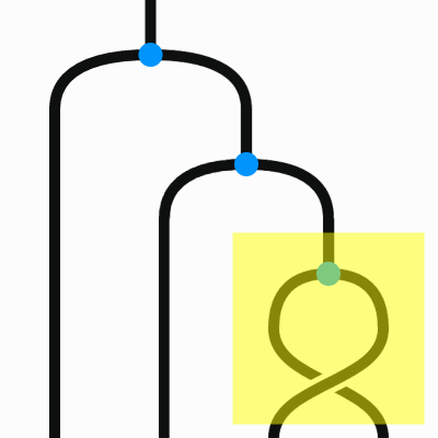
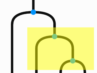
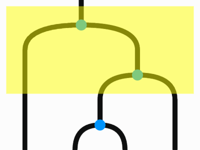
$\Rightarrow$		$\Rightarrow$		$\Rightarrow$		$\Rightarrow$		$\Rightarrow$		$\Rightarrow$

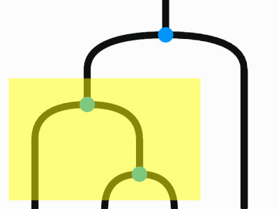
Figure 7: Absorption of the braid $\sigma_{1}\sigma_{2}^{-1}\sigma_{3}$.

Figure 8: The image of the 2-cell $\prod_{i=1}^{n}\sigma_{i}$ in the map of Definition 3.9. Steps 1 and 2 are creation and absorption of the braid $\sigma_{1}$ underneath the first tree; steps $2n-1$ and $2n$ are creation and absorption of the braid $\sigma_{n}$ under the last tree.

3.3 Theorem statement

Theorem 3.10.

The maps defined in Section 3.2 are (braided/symmetric) monoidal biequivalences.

Before commencing the proof of Theorem 3.10, we consider how the biequivalence results for braided and symmetric pseudomonoids in symmetric monoidal bicategories imply MacLane’s coherence theorems for braided and symmetric monoidal categories, which are braided and symmetric pseudomonoids in the symmetric monoidal bicategory Cat.

Corollary 3.11 (MacLane’s coherence theorems).

In a braided monoidal category, all diagrams of natural isomorphisms with the same underlying braid commute. In a symmetric monoidal category, all diagrams of natural isomorphisms with the same underlying permutation commute.

Proof (sketch).

First, note that these coherence theorems only refer to 2-cell diagrams internal to the category. From a 1-cell diagram in Cat, the only 1-cell data which are preserved internally are: the bracketing of the tree, the permutation of the tree’s input strings by the braid beneath the tree, and any units attached to the tree. From a 2-cell in Cat, the only generating 2-cells which are preserved internally are the associator, unitors, and commutator.

The case of a single tree is sufficiently general. The internal data underlying the diagram for the tree $f\in\mathrm{Hom}(\underline{m},{1})$ are $(\sigma,u,B)$, where $\sigma\in S_{m}$ is the permutation of the inputs by the braid underneath the tree, $u\in\mathbb{N}^{m+2}$ is a vector detailing the number of units between each input, and $B$ is a choice of bracketing of the resulting multiplication tree. Two diagrams are isomorphic without using the associator, unitors, or commutator if and only if they have the same internal data. Likewise, given internal data $(\sigma,u,B)$ we can define a diagram $D(\sigma,u,B)$ in Cat in a certain normal form which we will not detail precisely.

An internal 2-cell in a braided or symmetric monoidal category is a pasting diagram of associators, unitors and commutators which maps source internal data $(\sigma_{1},u_{1},B_{1})$ into target internal data $(\sigma_{2},u_{2},B_{2})$. Given such an internal 2-cell $L:(\sigma_{1},u_{1},B_{1})\to(\sigma_{2},u_{2},B_{2})$, we may define a movie $D(L):D(\sigma_{1},u_{1},B_{1})\to D(\sigma_{2},u_{2},B_{2})$ in Cat which executes it (the precise choice is irrelevant from the internal perspective).

Given two internal 2-cells $L_{1},L_{2}:(\sigma_{1},u_{1},B_{1})\to(\sigma_{2},u_{2},B_{2})$, consider the loop $D(L_{2})^{-1}D(L_{1})$. By Theorem 3.10:

• For a braided pseudomonoid, this loop is the identity if and only if the absorbed braid is trivial, indicating that the internal 2-cells are equal if and only if they have the same underlying braid.

• For a symmetric pseudomonoid, this loop is always the identity, indicating that two 2-morphisms inducing the same permutation $\sigma_{2}\sigma_{1}^{-1}$ are always equal.

∎

We now commence the proof of Theorem 3.10. We begin with some easy steps.

Lemma 3.12.

The maps described above are essentially surjective on objects.

Proof.

Clear; they are actually surjective. ∎

Lemma 3.13.

The maps described above are essentially surjective on 1-cells.

Proof.

The decategorified functors are isomorphisms, so there must be a chain of equalities reducing any 1-cell diagram to one in the image of the isomorphism. In the categorified setting these equalities become isomorphisms, which implies essential surjectivity. ∎

Lemma 3.14.

The maps described above are faithful on 2-cells.

Proof.

For the locally discrete bicategories, this is trivial. For ${\bf FS^{\text{br}}}$, note that the isotopy class of the braid absorbed by each tree is different for every 2-cell in the domain; since none of the generating 2-cells of the computad for a braided pseudomonoid in a symmetric Gray monoid change the isotopy class of the absorbed braid, the map must therefore be faithful on 2-cells. ∎

All that remains to show is that the maps are full on 2-cells and are functorial.

4 Proof of fullness

4.1 Putting the loop into normal form

We now demonstrate that the maps defined in the last section are full on 2-cells. To do this, we will provide an explicit series of rewrites that puts any loop on a 1-cell in the image of one of the maps into a normal form $N$ which we now define. Recall that ordered string diagrams in the image all consist of a braid (possibly trivial) followed by trees.

Definition 4.1.

The normal form $N$ is as follows: A braid (possibly trivial) is created directly beneath the leftmost tree, then absorbed according to Definition 3.9. This process is repeated for each tree, moving from left to right.

In Table 2 there are two variables: the braided structure of the ambient monoidal bicategory, and the braided structure of the pseudomonoid. Because of our choice of axioms, we need only consider the case of a braided pseudomonoid in a symmetric monoidal bicategory when defining our series of rewrites. This is because loops in other categories may be considered as loops in this Gray monoid which use only a restricted set of 1- and 2-cells. Only once we have rewritten the loop in the normal form $N$ will we need to distinguish the various cases.

Firstly we remove all unitors from the loop.

4.1.1 Removing unitors

Since there are no attached unit nodes in any 1-cell diagram in the image, any unit creation operator in the loop is paired with a unit destruction operator which destroys the created unit. The intuitive idea of the series of rewrites we are about to define is to move a unit creation operator towards the end of the loop, where at some point it will meet its paired destruction operator and the two can be cancelled. The process may then be iterated to remove all unit creation and destruction operators.

We first demonstrate how this can be done in a simple case.

Lemma 4.2.

Any unit creation operator may be eliminated along with its paired destruction operator if it satisfies the following conditions:

• The only 2-cells acting on the created multiplication 1-cell throughout the loop are its creation operator and its destruction operator.

• No further unit creation operators occur on the output string of the created unit 1-cell.

Proof.

The rewrite procedure is as follows.

1. Put the created unit in TSNF using Procedure 2.32.

2. Try to move the unit creation operator towards the end of the loop using Type I interchanger rewrites. The possible obstructions are as follows.

   • We have reached the paired destruction operator. Cancel the pair and we have finished.

   • A braiding inverse-insert, an inverse syllepsis, or a unit creation operator occurs at a vertical level between the created multiplication and the unit. Since the unit is in TSNF, and by assumption there are no further units created on the output string, this 2-cell will affect a rectangular subregion on one side of the unit’s output string. We may therefore:

     1. Insert interchangers and their inverses so that, after the 2-cell occurs, the unit interchanges upwards with the created 1-cells, and then returns.

     2. Use a Type III rewrite so that the 2-cell occurs below the unit, then the unit interchanges downwards.

     This reduces by one the number of 2-cells occuring between the two 1-cells.

   • A series of downwards interchangers and pullthroughs of the unit occurs. In this case, go to the last 2-cell in the series and try to delay it using Type I rewrites. If this is impossible, there must be an obstruction. If the obstruction is a 2-cell acting on the unit, then since only interchangers and pullthroughs act on the unit, the 2-cell must be an upwards interchanger or pullthrough. This may be cancelled with the downwards interchanger or pullthrough, reducing the number of interchangers and pullthroughs of the unit by two. If the 2-cell acts on the level directly above the unit, there are two possibilities, depending on what the 2-cell is:

     • A braiding inverse-insert, an inverse syllepsis or a unit creation operator at a level between the two 1-cells. Since the unit is in TSNF, and by assumption there are no further units created on the output string, this 2-cell will target a region on one side of the unit. We:

       1. Insert interchangers and their inverses so that, after the 2-cell occurs, the unit interchanges upwards with the created 1-cells, and then returns.

       2. Use a Type III rewrite so that the 2-cell occurs below the unit, then the unit interchanges downwards.

       This reduces by one the number of 2-cells occuring between the multiplication and the unit.

     • Any other 2-cell. In this case, the interchanger will have interchanged downwards with all the involved 1-cells; we may therefore use a Type III rewrite, reducing by one the number of 2-cells occuring between the multiplication and the unit.

3. Iterate the procedure. Since all paths above either cancel the unit creation and destruction operators, reduce the number of interchangers of the unit, or reduce the the number of 2-cells occuring at a level between the two 1-cells, it is clear that this result in cancellation of the creation and destruction operators.

∎

Example 4.3.

See the 5-cell ‘Example 4.3 - Statement’ and the 6-cell ‘Example 4.3 - Pf’ in the Globular workspace. The first 20 rewriting steps put the created unit into TSNF, and the remaining 26 steps eliminate it.

Definition 4.4.

We call unit creation operators satisfying the conditions of Lemma 4.2 unnested with fixed multiplication.

We now show how to rewrite any loop so that the final unit creation operator is unnested with fixed multiplication.

Lemma 4.5.

Any loop can be rewritten so that the last unit creation operator is unnested with fixed multiplication, without increasing the number of unit creation operators.

Proof.

The last unit creation operator is clearly unnested. We now show how to fix the created multiplication node without introducing nesting. Consider the first 2-cell involving the created multiplication 1-cell. If this 2-cell is a unit destruction operator then we are finished. If not:

1. Insert interchangers, pullthroughs and their inverses (IPI) immediately prior to the 2-cell so that the unit node goes straight up to the multiplication 1-cell, returns to where it started and then the 2-cell occurs.

2. Insert a unit destruction operator and its inverse immediately before the pulldowns.

3. Eliminate the first unit creation operator and the inserted destruction operator using Lemma 4.2. We can do this since by assumption this was the first 2-cell acting on the created unit, and the unit is unnested.

4. Use Type I rewrites so that the 2-cell occurs immediately after the unit creation (or after additional interchangers/pullthroughs if necessary).

We now have a movie with the same number of unit creation operators where the last creation operator occurs, the unit interchanges or pulls through downwards to directly beneath the region acted on by the 2-cell involving the multiplication, and then the 2-cell occurs. We now show how to eliminate each possible 2-cell case-by-case.

• The multiplication interchanges downwards. In this case the creation operator occurs and then both the unit and the multiplication interchange once downwards. Use a Type III rewrite so that the creation operator occurs immediately below the 1-cell involved in the interchanger:

  $[$

  $\Rightarrow$ $\Rightarrow$ $\Rightarrow$

  $]$

  $=$

  $[$

  $\Rightarrow$ $]$

• The multiplication interchanges upwards. In this case the creation operator occurs and then the multiplication interchanges upwards. Insert a upwards interchanger of the unit and its inverse immediately following the upwards interchanger of the multiplication. Use a Type II then a Type III rewrite so that the creation operator occurs immediately above the 1-cell involved in the interchanger:

  $[$ $\Rightarrow$ $\Rightarrow$ $]$

  $=$

  $[$ $\Rightarrow$ $\Rightarrow$ $]$

• The multiplication pulls through downwards. In this case the creation operator occurs immediately above a braiding, the unit pulls through, and is followed by the multiplication node. Use $(\cdot\otimes\Rightarrow)$ or $(\Rightarrow\otimes\cdot)$ so that the creation operator occurs beneath the braiding:

  $[$ $\Rightarrow$ $\Rightarrow$ $\Rightarrow$ $\Rightarrow$ $]$

  $=$

  $[$ $\Rightarrow$ $]$

• The multiplication pulls through upwards. Here the creation operator occurs immediately below a braiding, and the multiplication then pulls through upwards. Insert an upwards pullthrough of the unit followed by a downwards pullthrough immediately after the pullthrough of the multiplication. Use $(\cdot\otimes\Rightarrow)$ or $(\Rightarrow\otimes\cdot)$ so that the creation operator occurs above the braiding and the unit then pulls through downwards:

  $[$ $\Rightarrow$ $\Rightarrow$ $]$

  $=$

  $[$ $\Rightarrow$ $\Rightarrow$ $\Rightarrow$ $]$

• The multiplication is the lower partner in an associator or inverse associator. In this case the creation operator is performed immediately below a multiplication 1-cell, with which the created multiplication 1-cell immediately associates. Here we require four equalities, all of which are implied by the triangle equality. Two are shown below; the others are the same, but with all diagrams flipped in a vertical axis (we call them (A1V) and (A2V).

  $[$ $\Rightarrow$ $\Rightarrow$ $]$	$=$	$[$ $\Rightarrow$ $\Rightarrow$ $]$	(A1)
  $[$ $\Rightarrow$ $\Rightarrow$ $]$	$=$	$[$ $\Rightarrow$ $]$	(A2)

  The full derivations of these rewrites can be found in the Globular workspace as the 6-cells ‘Lemma 4.5 - Mult lower partner in associator Pf (A1)’ and ‘Lemma 4.5 - Mult lower partner in associator Pf (A2)’. In the proof we use two intermediate lemmas, the 5-cells ‘Lemma 4.5 - Associator Lemma Left’ and ‘Lemma 4.5 - Associator Lemma Right’. We give the proof for the left lemma as the 6-cell ‘Lemma 4.5 - Associator Lemma Left Pf’; the proof for the right lemma is similar.

• The multiplication is the upper partner in an associator or inverse associator. Here the unit creation operator occurs directly above a multiplication 1-cell, the unit interchanges downwards, and an associator or inverse associator is then performed. For a left unit, this will be an associator, and for a right unit it will be an inverse associator. We require two equalities, one of which is (A1) postcomposed on both sides with an inverse associator, and the other of which is (A1V) postcomposed on both sides of the equality with an associator.

• The multiplication annihilates with another unit. In this case, the creation operator occurs directly above a unit. The created unit then interchanges downwards and the multiplication annihilates with the other unit. To rewrite this movie we need one equality for a left unit creation, derivable from the triangle equality. The equality for a right unit creation is simply the flip of this one.

  $[$ $\Rightarrow$ $\Rightarrow$ $\Rightarrow$ $]$

  $=$

  $[$ $]$

  We provide the full derivation of this equality in the Globular workspace as the 6-cell ‘Lemma 4.5 - Left unit twist Pf’. For convenience, we include the 5-cell ‘Lemma 4.5 - Right unit twist’ separately.

• The multiplication is acted on by a commutator or inverse commmutator. For a commutator the unit is created, pulls through the other string, and a commutator occurs. For an inverse commutator, the unit is created and then an inverse commutator occurs. One equality for a commutator is shown below; the other equality is the same, but with all diagrams flipped in a vertical axis. The two equalities for inverse commutators follow from the equalities for commutators by flipping and then postcomposing on both sides with a unit creation and a pullthrough.

  $[$ $\Rightarrow$ $\Rightarrow$ $\Rightarrow$ $]$

  $=$

  $[$ $\Rightarrow$ $]$

  The full derivation of this rewrite is shown in the Globular workspace as ‘Lemma 4.5 - Commutator Lemma Pf’.

All these rewrites remove the first 2-cell on the multiplication 1-cell. The result therefore follows by iterating the procedure. ∎

Using these results together, we may remove all unitors.

Proposition 4.6.

Any loop on a 1-morphism in the image of $F$ may be rewritten so that it contains no unit creation or destruction operators.

Proof.

Use Lemma 4.5 to rewrite the movie such that the last unit creation operator is unnested with fixed multiplication; then eliminate it using Lemma 4.2. Repeat until all unit creation operators have been removed. ∎

4.1.2 Fixing the trees

We now have a loop consisting only of associators, interchangers, commutators, pullthroughs, syllepses, braiding inverse-inserts and braiding cancellations. Recall that the source 1-cell diagram of the loop is a braiding followed by a series of left-bracketed multiplication trees with heights rising from left to right, where we consider a unit 1-cell to be a multiplication tree $m^{0}$. We will now provide a series of rewrites that will ‘fix the trees’. The intuitive meaning of this is shown in Figure LABEL:fixedtreesfigure.