The Sun in transition? Persistence of near-surface structural changes through Cycle 24

Abstract

We examine the frequency shifts in low-degree helioseismic modes from the Birmingham Solar-Oscillations Network (BiSON) covering the period from 1985 – 2016, and compare them with a number of global activity proxies well as a latitudinally-resolved magnetic index. As well as looking at frequency shifts in different frequency bands, we look at a parametrization of the shift as a cubic function of frequency. While the shifts in the medium- and high-frequency bands are very well correlated with all of the activity indices (with the best correlation being with the 10.7 cm radio flux), we confirm earlier findings that there appears to have been a change in the frequency response to activity during solar cycle 23, and the low-frequency shifts are less correlated with activity in the last two cycles than they were in Cycle 22. At the same time, the more recent cycles show a slight increase in their sensitivity to activity levels at medium and higher frequencies, perhaps because a greater proportion of activity is composed of weaker or more ephemeral regions. This lends weight to the speculation that a fundamental change in the nature of the solar dynamo may be in progress.

1 INTRODUCTION

The current solar activity Cycle 24 has been significantly weaker than the previous few cycles (e.g., see Hathaway, 2015). These changes were signposted by the unusually extended and deep solar minimum at the boundary of Cycles 23 and 24. Very few of the predictions collated by the Solar Cycle 24 Prediction Panel (Pesnell, 2008, 2012) forecast the extent of the minimum or the low levels of activity that followed.

One must go back around one-hundred years to find cycles that show levels of activity as low as those observed in Cycle 24, e.g., Cycles 14 and 15 both provide very good matches in traditional proxies such as the International Sunspot Number (ISN). Tellingly, this earlier epoch pre-dates both the modern Grand Maximum period and the satellite era. The wide range of contemporary observations and data products was therefore not available to characterize and study the Sun during that era.

Some activity indicators dropped to remarkably low values during the Cycle 23/24 minimum (e.g. the geomagnetic $aa$-index and the ISN). Solar wind turbulence, as captured by measures of interplanetary scintillation, had been declining since the early part of Cycle 23. There have been results suggesting a decline – from the Cycle 23/24 boundary through the rise of Cycle 24 – in the average strength of magnetic fields in sunspots (Livingston et al. 2012; see also Watson et al. 2014) and others pointing to a change in the size distribution of spots between Cycles 22 and 23 (e.g., see Clette & Lefèvre, 2012; de Toma et al., 2013).

Helioseismic studies of the internal solar dynamics showed that the characteristics of the meridional flow altered between Cycles 23 and 24 (Hathaway & Rightmire, 2010). Changes to the meridional flow have potential consequences for flux-transport dynamo models. Differences have also been seen in the east-west zonal flows (e.g., Howe et al., 2013) and in the frequency shifts of globally coherent p modes, which have been weaker than in preceding cycles (e.g., see Basu et al., 2012; Salabert et al., 2015; Tripathy et al., 2015; Howe et al., 2015).

Upton & Hathaway (2014) have suggested that it was actually a weak Cycle 23 that was responsible for the following, extended minimum and weak Cycle 24. Jiang et al. (2015) have proposed that observed weak polar magnetic fields, and as a result the weak Cycle 24, may have resulted from the emergence of low-latitude flux having the opposite polarity to that expected (which then hindered growth of the polar fields). Predictions for Cycle 25 are now beginning to appear (e.g., see Pesnell, 2016).

Around the time of the early stages of Cycle 24, we used helioseismic data collected by the Birmingham Solar-Oscillations Network (BiSON) to uncover clear signs of unusual behaviour in the near-surface layers that appeared as far back as the latter stages of Cycle 22 (Basu et al., 2012). We analysed the cycle-induced frequency shifts shown by modes in three different frequency bands of the p-mode spectrum. The relationship of the frequency shifts to the ISN and the 10.7-cm radio flux – the latter another commonly used proxy of global solar activity – changed noticeably, and the close correlation with the indices was lost during a period stretching from the tail end of Cycle 22 through the Cycle 23 maximum (with the lowest-frequency modes losing the correlation first). Whilst the correlation recovered for modes above $\simeq 2400\,\rm\mu Hz$, it failed to do so for the lower-frequency modes. The results imply an underlying change in structure very close to the surface, where the lower-frequency cohort is less sensitive to perturbations. We showed that one may interpret the structural change in terms of a thinning of the layer of near-surface magnetic field, post-Cycle 22.

These helioseismic markers were sufficiently robust that, with the benefit of hindsight, they arguably may have provided an early warning of the changes that would be seen in other proxies as the Sun headed into Cycle 24. At the time of writing, Cycle 24 is about half-way down its declining phase. Our goal in this paper is, therefore, to use the up-to-date BiSON data to test whether the unusual behaviour uncovered by our previous analysis has persisted through the declining phase of the cycle, and what the results might mean for Cycle 25. The rest of the paper is laid out as follows. Details on the data used, and the analysis performed, are given in Section 2. We discuss results on the extracted frequency shifts and activity proxies in Section 3, including a new way of presenting the information encapsulated in the frequency shifts. We finish the paper in Section 4 by discussing the implications of the results, not only for Cycle 25, but also in the wider context of the activity behaviour of Sun-like stars.

2 Data and Analysis

The six telescopes comprising BiSON make unresolved “Sun-as-a-star” observations of the visible solar disc (Chaplin et al., 1996; Hale et al., 2016), and thereby provide data that are sensitive to the globally coherent, low angular-degree (low-$l$) solar p modes. Whilst these modes are formed by acoustic waves that penetrate the solar core, they are very sensitive to perturbations in the near-surface layers and hence provide a useful diagnostic and probe of the global response of the Sun to changing levels of solar activity and the resulting near-surface structural changes.

The BiSON observations constitute a unique database that now stretches over four 11-year solar activity cycles, i.e., from Cycle 21 through to the falling phase of the current Cycle 24. The observations we use here span the period 1985 July 2 through 2016 December 31, or in other words Cycles 22, 23, and most of 24; the data from Cycle 21 are too sparse to be suitable for the current analysis. The raw Doppler velocity data were prepared for analysis using the procedures described by Davies et al. (2014a, b), and then they were divided into overlapping subsets of length 365 days, offset by 91.25 days. The frequency-power spectrum of each subset was fitted to a multi-parameter model to extract estimates of the low-$l$ mode frequencies. Details can be found in Howe et al. (2015), but while that paper used two different codes to extract the frequencies, for this work we used only frequencies estimated using the more sophisticated method, a Markov-Chain Monte-Carlo sampler. We deliberately re-analyzed the entire database in order to verify, using independent analysis codes, the results presented by Basu et al. (2012).

Having extracted the individual frequencies, we then followed the procedure outlined by Basu et al. (2012) to extract averaged frequency shifts for each 365-day segment, in three frequency bands. The bands cover low ($1860<\nu_{nl}\leq 2400\,\rm\mu Hz$), medium ($2400<\nu_{nl}\leq 2920\,\rm\mu Hz$) and high frequencies ($2920<\nu_{nl}\leq 3450\,\rm\mu Hz$). The reference frequencies used for computing the variations came from averages of the frequencies for the 13 subsets straddling the Cycle 22 maximum (spanning the dates 1988 October 1 to 1992 April 30).

In addition to using averaged frequency shifts, we also used results from parametrizing the frequency shifts as a function of frequency (Gough 1990; see also Howe et al. 2017). The frequency shifts of individual modes, $\delta\nu_{nl}(t)$, were first scaled by the mode inertia, $E_{nl}$, of model “S” of Christensen-Dalsgaard et al. (1996). This removes the dependence of the shifts on inertia, leaving signatures due to perturbations in the near-surface layers. The scaled shifts of each 365-day subset were then fitted to a parametrized one or two-term function in frequency $\nu$, i.e.,

$$\mathcal{F}(\nu)=a_{\rm inv}\left(\frac{\nu}{\nu_{\rm ac}}\right)^{-1}+a_{\rm cub}\left(\frac{\nu}{\nu_{\rm ac}}\right)^{3},$$ (1)

or in the one-term case simply

$$\mathcal{F}(\nu)=a_{\rm cub}\left(\frac{\nu}{\nu_{\rm ac}}\right)^{3},$$ (2)

where $\nu_{ac}$ is the acoustic cut-off frequency of 5 mHz. The fit yields best-fitting coefficients $a_{\rm cub}$, and optionally $a_{\rm inv}$, for each subset. The rationale given by Gough (1990) for this choice of terms is, briefly, that the cubic term corresponds to a modification of the propagation speed of the waves by a fibril magnetic field close to the surface, as also suggested by Libbrecht & Woodard (1990), while the inverse term would correspond to a change in scale height in the superadiabatic boundary layer.

For the low-degree data we found that the $a_{\rm inv}$ term was not statistically significant, so here we work with the cubic term only.

The averaged frequency shifts for each band, and the best-fitting coefficients from the cubic-function parametrization of the shifts, constitute our core helioseismic diagnostic data.

3 Results

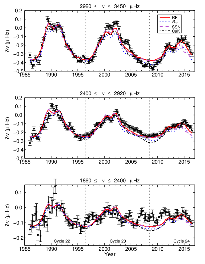
Figure 1: Averaged frequency shifts (symbols with error bars) in each of three frequency bands as a function of time. Also plotted are data on the 10.7-cm radio flux (solid red curve), CaK index (black dash-dotted curve), Kitt Peak global magnetic field strength index (dotted blue curve) and ISN (purple dashed curve), all scaled to the frequency shifts from the maximum and descending phase of Cycle 22 (see text). The vertical dotted lines indicate the cycle minima.

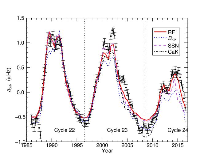
Figure 2: Extracted coefficients $a_{\mathrm{cubic}}$, from the cubic parametrization of the frequency shifts, as a function of time. Also plotted are data on the 10.7-cm radio flux (red solid curve), CaK index (black dash-dotted curve), global magnetic field strength index (blue dotted curve) and ISN (purple dashed curve), scaled to the frequency shifts in Cycle 22 (see text). The vertical dotted lines indicate the cycle minima.

Fig. 1 shows the extracted averaged frequency shifts in each band as a function of time. Also plotted are data on the 10.7-cm radio flux (Tapping, 2013) , the revised Brussels-Locarno Sunspot Number (Clette et al., 2016), a merged CaK index(Bertello et al., 2016) and a global magnetic field-strength index based on Kitt Peak synoptic magnetogram data (see Howe et al., 2017, for details), each averaged over the same epochs as the frequencies, and scaled by a linear fit to the frequency shifts over the maximum and descending phase of Cycle 22, (i.e, the date range from 1990.0 to 1996.5). Fig. 2 shows the extracted coefficients $a_{\rm cub}$, as a function of time, with the radio-flux, sunspot, CaK, and magnetic data overplotted, again scaled by a linear fit to the cubic coefficients in the latter part of Cycle 22.

Signatures of the 11-year solar activity cycle are the dominant feature of both sets of diagnostics. However, both frequencies and activity proxies also show some shorter-term variability with an average period of around 2 years. This periodicity is a known feature of several global proxies of solar activity (e.g., see Bazilevskaya et al., 2014) and has been detected in a number of helioseismic datasets (e.g., see Fletcher et al., 2010; Broomhall et al., 2012; Simoniello et al., 2012, 2013). Following Basu et al. (2012), we have removed shorter-period variations, including the 2-year signal, by smoothing the respective sets of averaged frequency shifts and extracted coefficients over nine samples or 2.25 years. The resulting smoothed diagnostic data are plotted in Fig. 3 for the average frequency shifts and Fig. 4 for the cubic coefficients, together with smoothed and scaled versions of the activity proxies.

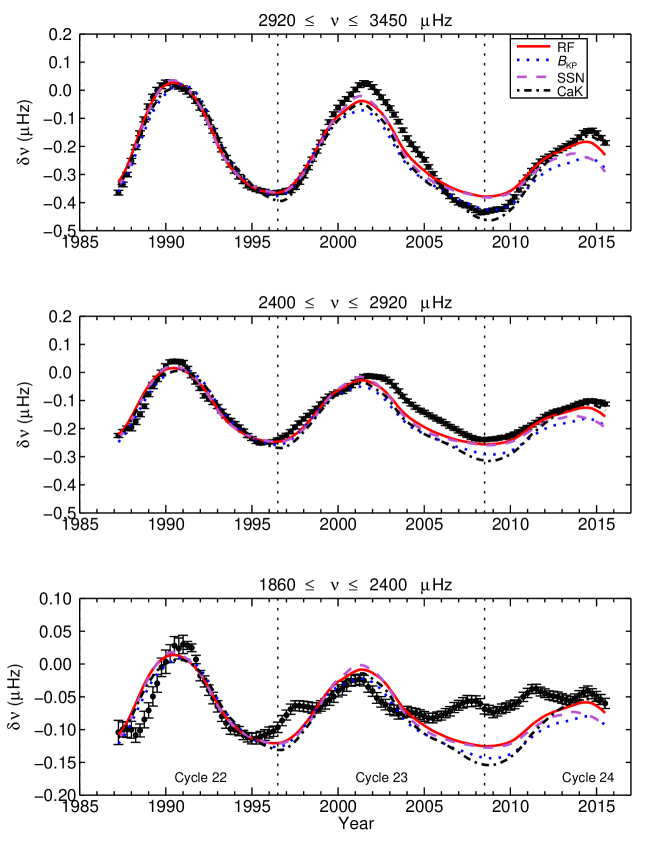
Figure 3: Averaged frequency shifts (symbols) in each of three frequency bands as a function of time, but after smoothing to remove shorter-term variations. Also plotted are data on the 10.7-cm radio flux (red solid curve), ISN (purple dashed curve), CaK index (black dash-dotted curve) and global magnetic index (blue dotted curve), all scaled by a linear fit to the smoothed frequency shifts over the maximum and descending phase of Solar Cycle 22 (see text). The vertical dotted lines indicate the cycle minima.

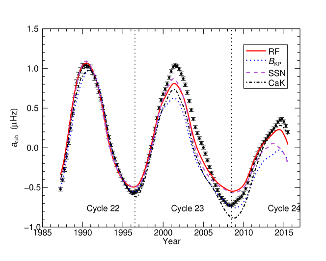
Figure 4: Coefficient $a_{\rm cubic}$, as a function of time but after smoothing the data to remove shorter-term variations. Also plotted are data on the 10.7-cm radio flux (red solid curve), CaK index (black dash-dotted curve), ISN (purple dashed line), and magnetic global index (blue dotted curve) (see text), scaled by a linear fit to the smoothed $a_{\rm cubic}$ coefficients over the maximum and descending phase of Solar Cycle 22. The vertical dotted lines indicate the cycle minima.

Figures 1 and  3 correspond to Figures 2 and 3 of Basu et al. (2012), with the slight difference that we have scaled the activity proxies to the frequencies over a wider range in time, while the cubic-fit coefficients in Figures 2 and 4 combine data from all three bands but are more heavily weighted towards the higher-frequency modes. The first important point to make is that our re-analysis of the BiSON data confirms the results presented in Basu et al. (2012), although there are some differences in detail that may be due to the improved frequency estimation. Prior to $\simeq 1994$, during the latter stages of Cycle 22, changes in the frequencies followed reasonably closely the variations shown by the global activity proxies. However, at epochs thereafter, the behaviour of the frequency shifts in the low-frequency band departed strongly from the proxies, with detected variations in the frequencies being much weaker than expected (based on the behaviour seen in Cycles 21 and 22); in particular, these frequencies stayed higher than expected during the very low-activity period of the minimum following Cycle 23. We also note that the relationship between the radio flux and sunspot data temporarily changed during the declining phase of Cycle 23 (as pointed out by Tapping & Valdés 2011; see also Clette et al. 2016 for comments on the comparison with the newly recalibrated sunspot data).

Our new results extend the observations into the declining phase of Cycle 24, and they show clearly that the significant departures seen at low frequencies have persisted as we head towards the onset of the next cycle. Put another way, the acoustic properties of the near-surface layers have failed to re-set to their pre-1994 state. While for the mid- and high-frequency band shifts and the cubic parametrization coefficient the correlation with the activity indices does appear to recover in the rising phase of Cycle 24, the shifts again deviate from the extrapolated fit to Cycle 22 in the most recent data corresponding to the declining phase of Cycle 24, at least for the RF, magnetic, and sunspot indices. We note that the scaled RF and sunspot proxies show very similar behaviour except in the declining phase of Cycle 24, while the CaK and magnetic proxies are fairly close to one another. While the magnetic and CaK proxies fall to noticeably lower levels during the Cycle 23/24 minimum than during the previous minimum, the difference between the minima is less pronounced for the RF and sunspot number. Interestingly, the frequency shifts in the high-frequency band, as well as the cubic-fit coefficients, appear to follow the magnetic and CaK pattern, while the frequency shifts in the middle band follow the RF and sunspot number and the low-frequency band is not a good match to any of the proxies in this period. During the maximum epoch of Cycle 24 the frequencies in the high and middle bands seem to follow the extrapscaled RF and CaK proxies while the sunspot and magnetic proxies show poorer agreement, and in the declining phase so far only the CaK looks like a good match to the frequency shifts. We emphasise that all of the proxies have been scaled to match the relationship to the frequency shifts that was seen in the 1990 – 1996.5 epoch; better fits could be obtained by fitting to each cycle separately. The difference in behaviour at the Cycle 23/4 minimum is striking, however, and it is not an artefact of the scaling. Broomhall (2017) also found that the medium-degree frequencies from the Global Oscillation Network Group were systematically lower during this minimum than during the previous one, as would be expected when the fields are weaker.

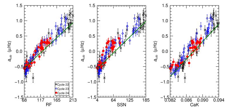
Figure 5: Cubic coefficient for $l=0$ only, plotted against different global activity indices, for solar cycles 22 (black crosses), 23 (blue open diamonds), and 24 (red filled circles). The solid line indicates a linear fit to the data between 1990 and 1996, i.e. the maximum and descending phase of Cycle 22.

Because the BiSON observations are primarily sensitive to the sectoral, or $m=l$ modes, we can expect the frequency shifts for $l\geq 1$ to show some hysteresis with global activity measures. To examine the impact this may have on our results, we carried out the frequency-cubed parametrization for each $l$ separately. Figure 5 shows the unsmoothed cubic coefficient derived from fits to the $l=0$ shifts only, plotted against each of the three unresolved activity indices and colour-coded by cycle. Also shown is a straight line representing the extrapolation of a linear fit to the Cycle 22 data after 1990. In each case, it can be seen that the data for the Cycle 23 and 24 maxima lie generally above the line. This suggests that in the two most recent cycles we are seeing a larger shift overall for the same amount of activity than we did in Cycle 22, in the middle and higher frequency bands that dominate the cubic fit. This might make sense if there has been a shift towards a greater proportion of weak, ephemeral activity that does not register in the sunspot number or on the synoptic magnetic charts but could still have an influence on the modes. The numerical results of fits between the $l=0$ cubic coefficient and the activity proxies, for each cycle individually and for the entire data sets, are given in Table 1.

In the case of the magnetic proxy, we do have information on the latitudinal distribution of activity in the synoptic magnetograms, and we can use this to derive an index appropriate to the sectoral mode at each value of $l$ (see, for example, Chaplin et al., 2004). In Figure 6 we show the cubic coefficients for each $l$ separately as a function of the projection of the latitudinal field-strength distribution on the corresponding $m=l$ spherical harmonic. The results of linear fits to the magnetic proxy for each cycle separately and for the whole dataset are shown in Table 2. Again, we can see that the points corresponding to the maxima of Cycles 23 and 24 lie above the curve indicating the trend in Cycle 22, so we cannot attribute the hysteresis we observe in the averaged frequencies simply to the latitudinal distribution of activity. The $l=3$ points from early Cycle 22 that lie well below the line are probably due to poor fits of these modes (to which a Sun-as-a-star instrument like BiSON is not very sensitive) in the low duty cycle of the early observations.

Table 1: Results of linear fits between global proxies and cubic frequency-shift coefficient for $l=0$, for the three cycles individually and the whole period. These fits were carried out for non-overlapping data only.

Proxy	Period	Intercept ($\mu$Hz)	Slope ($\mu$Hz/activity unit)	$\chi^{2}$	$R$
RF	Cycle 22	$(-1.266\pm 0.096)\times 10^{0}$	$(1.080\pm 0.073)\times 10^{-2}$	2.59160	0.946495
”	Cycle 23	$(-1.498\pm 0.096)\times 10^{0}$	$(1.310\pm 0.077)\times 10^{-2}$	1.13799	0.980589
”	Cycle 24	$(-1.323\pm 0.163)\times 10^{0}$	$(1.197\pm 0.151)\times 10^{-2}$	0.725496	0.967366
”	All	$(-1.344\pm 0.060)\times 10^{0}$	$(1.178\pm 0.049)\times 10^{-2}$	1.59291	0.958641
SSN	Cycle 22	$(-5.675\pm 0.560)\times 10^{-1}$	$(8.866\pm 0.601)\times 10^{-3}$	2.82573	0.941283
”	Cycle 23	$(-5.982\pm 0.496)\times 10^{-1}$	$(1.003\pm 0.060)\times 10^{-2}$	2.14756	0.963345
”	Cycle 24	$(-4.994\pm 0.718)\times 10^{-1}$	$(1.137\pm 0.161)\times 10^{-2}$	2.88601	0.858331
”	All	$(-5.227\pm 0.308)\times 10^{-1}$	$(9.204\pm 0.397)\times 10^{-3}$	2.75214	0.933063
CaK	Cycle 22	$(-1.368\pm 0.093)\times 10^{1}$	$(1.563\pm 0.106)\times 10^{2}$	2.87813	0.943093
”	Cycle 23	$(-1.497\pm 0.089)\times 10^{1}$	$(1.728\pm 0.102)\times 10^{2}$	1.35981	0.975541
”	Cycle 24	$(-1.030\pm 0.129)\times 10^{1}$	$(1.185\pm 0.150)\times 10^{2}$	0.780809	0.965822
”	All	$(-1.327\pm 0.056)\times 10^{1}$	$(1.526\pm 0.065)\times 10^{2}$	2.14424	0.946690

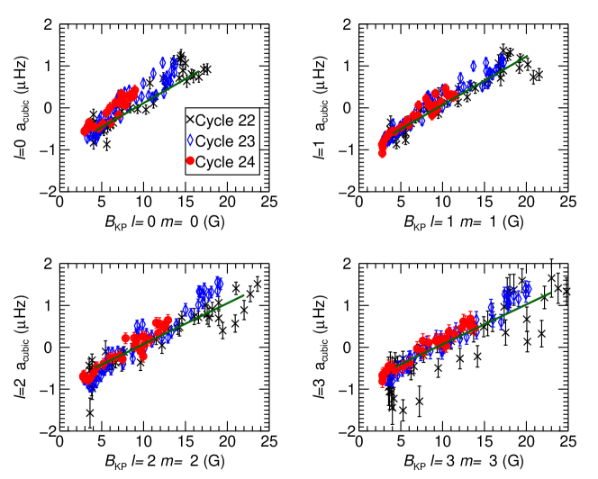
Figure 6: Cubic coefficients for fits to MCMC scaled frequency shifts for individual $l$ plotted as a function of the $l,m=l$ projection of the magnetic field strength, for solar cycles 22 (black crosses), 23 (blue open diamonds), and 24 (red filled circles).

Table 2: Results of linear fits between $m=l$ components of the Kitt Peak magnetic index and the cubic frequency-shift coefficient for each l, for the three cycles individually and the whole period.

$l$	Period	Intercept ($\mu$Hz)	Slope ($\mu$Hz/G)	$\chi^{2}$	$R$
0	Cycle 22	$-0.990\pm 0.081$	$0.119\pm 0.081$	4.153	0.918
0	Cycle 23	$-1.111\pm 0.076$	$0.147\pm 0.076$	2.596	0.954
0	Cycle 24	$-0.944\pm 0.117$	$0.143\pm 0.117$	0.842	0.963
0	All	$-0.950\pm 0.047$	$0.126\pm 0.006$	3.187	0.921
1	Cycle 22	$-1.025\pm 0.072$	$0.112\pm 0.072$	2.588	0.959
1	Cycle 23	$-1.044\pm 0.067$	$0.124\pm 0.067$	2.614	0.963
1	Cycle 24	$-1.237\pm 0.096$	$0.144\pm 0.096$	2.858	0.940
1	All	$-1.063\pm 0.042$	$0.121\pm 0.004$	2.627	0.955
2	Cycle 22	$-0.953\pm 0.090$	$0.101\pm 0.090$	0.855	0.965
2	Cycle 23	$-1.299\pm 0.080$	$0.145\pm 0.080$	3.575	0.958
2	Cycle 24	$-1.084\pm 0.113$	$0.127\pm 0.113$	2.056	0.938
2	All	$-1.106\pm 0.051$	$0.124\pm 0.005$	2.629	0.938
3	Cycle 22	$-1.085\pm 0.149$	$0.107\pm 0.149$	2.430	0.913
3	Cycle 23	$-1.118\pm 0.100$	$0.122\pm 0.100$	1.079	0.969
3	Cycle 24	$-1.047\pm 0.133$	$0.122\pm 0.133$	0.836	0.966
3	All	$-1.072\pm 0.068$	$0.117\pm 0.007$	1.433	0.917

4 Discussion

We have used the latest BiSON helioseismic data to show that previously uncovered changes in the structure of the near-surface layers of the Sun, which date back to the latter stages of Cycle 22 (around 1994), have persisted through the declining phase of the current, weak Cycle 24. The acoustic properties have as such failed to re-set to their pre-1994 state. While the agreement at higher frequencies did appear to recover in the rising phase of Cycle 24, when the most recent data are added we can see that there are again differences from the proxies extrapolated from Cycle 22. This supports the suggestion of Basu et al. (2012) that the magnetic changes affecting the Cycle 23 (and later) oscillation frequencies were confined to a thinner layer than those in Cycle 22.

We also find that the sensitivity of the frequencies in the higher-frequency bands to the magnetic proxy is slightly higher in the two most recent cycles than in Cycle 22, which could be due to a higher proportion of weaker, more ephemeral active regions that are not accounted for in the synoptic magnetic data. This observation still holds when we separate out the frequency shifts by degree and compare with a latitudinally resolved magnetic proxy.

It is tempting to speculate whether these results, and the multitude of other unusual signatures relating to Cycle 24, might be indicative of a longer-lasting transition in solar activity behaviour, and the operation of the solar dynamo.

The existence of the Maunder Minimum, and other similar minima suggested by proxy data relevant to millennal timescales, indicate that there have likely been periods when the action of the dynamo has been altered significantly. We finish by speculating whether these events might presage a radical transition suggested by data on other stars. Results on activity cycle periods shown by other stars hint at a change in cycle behaviour – a possible transition from one type of dynamo action to another – at a surface rotation period of around 20 days (Böhm-Vitense, 2007). There is also more recent intriguing evidence from asteroseismic results on solar-type stars (van Saders et al., 2016; Metcalfe et al., 2016) that shows that the spin-down behaviour of cool stars changes markedly once they reach a critical epoch, with the corresponding surface rotation period depending on stellar mass. For solar-mass stars, the results suggest a change in behaviour at about the solar age (and solar rotation period).

ACKNOWLEDGMENTS

We would like to thank al those who are, or have been, associated with BiSON, in particular P. Pallé and T. Roca-Cortes in Tenerife and E. Rhodes Jr. and S. Pinkerton at Mt. Wilson. BiSON is funded by the Science and Technology Facilities Council (STFC), under grant ST/M00077X/1. SJH, GRD, YPE, and RH acknowledge the support of the UK Science and Technology Facilities Council (STFC). Funding for the Stellar Astrophysics Centre (SAC) is provided by The Danish National Research Foundation (Grant DNRF106). NSO/Kitt Peak data used here were produced cooperatively by NSF/NOAO, NASA/GSFC, and NOAA/SEL; SOLIS data are produced cooperatively by NSF/NSO and NASA/LWS. RH thanks the National Solar Observatory for computing support. SB acknowledges National Science Foundation (NSF) grant AST-1514676.

References

- Basu et al. (2012) Basu S., Broomhall A.-M., Chaplin W. J., Elsworth Y., 2012, ApJ, 758, 43
- Bazilevskaya et al. (2014) Bazilevskaya G., Broomhall A.-M., Elsworth Y., Nakariakov V. M., 2014, Space Sci. Rev., 186, 359
- Bertello et al. (2016) Bertello L., Pevtsov A., Tlatov A., Singh J., 2016, Solar Physics, 291, 2967
- Böhm-Vitense (2007) Böhm-Vitense E., 2007, ApJ, 657, 486
- Broomhall (2017) Broomhall A.-M., 2017, preprint, (arXiv:1702.03149)
- Broomhall et al. (2012) Broomhall A.-M., Chaplin W. J., Elsworth Y., Simoniello R., 2012, MNRAS, 420, 1405
- Chaplin et al. (1996) Chaplin W. J., et al., 1996, Sol. Phys., 168, 1
- Chaplin et al. (2004) Chaplin W. J., Elsworth Y., Isaak G. R., Miller B. A., New R., 2004, MNRAS, 352, 1102
- Christensen-Dalsgaard et al. (1996) Christensen-Dalsgaard J., et al., 1996, Science, 272, 1286
- Clette & Lefèvre (2012) Clette F., Lefèvre L., 2012, Journal of Space Weather and Space Climate, 2, A06
- Clette et al. (2016) Clette F., Lefèvre L., Cagnotti M., Cortesi S., Bulling A., 2016, Solar Physics, 291, 2733
- Davies et al. (2014a) Davies G. R., Broomhall A. M., Chaplin W. J., Elsworth Y., Hale S. J., 2014a, MNRAS, 439, 2025
- Davies et al. (2014b) Davies G. R., Chaplin W. J., Elsworth Y., Hale S. J., 2014b, MNRAS, 441, 3009
- Fletcher et al. (2010) Fletcher S. T., Broomhall A.-M., Salabert D., Basu S., Chaplin W. J., Elsworth Y., Garcia R. A., New R., 2010, ApJ, 718, L19
- Gough (1990) Gough D. O., 1990, in Osaki Y., Shibahashi H., eds, Lecture Notes in Physics, Berlin Springer Verlag Vol. 367, Progress of Seismology of the Sun and Stars. p. 283, doi:10.1007/3-540-53091-6
- Hale et al. (2016) Hale S. J., Howe R., Chaplin W. J., Davies G. R., Elsworth Y. P., 2016, Sol. Phys., 291, 1
- Hathaway (2015) Hathaway D. H., 2015, Living Reviews in Solar Physics, 12, 4
- Hathaway & Rightmire (2010) Hathaway D. H., Rightmire L., 2010, Science, 327, 1350
- Howe et al. (2013) Howe R., Christensen-Dalsgaard J., Hill F., Komm R., Larson T. P., Rempel M., Schou J., Thompson M. J., 2013, ApJ, 767, L20
- Howe et al. (2015) Howe R., Davies G. R., Chaplin W. J., Elsworth Y. P., Hale S. J., 2015, MNRAS, 454, 4120
- Howe et al. (2017) Howe R., Basu S., Davies G. R., Ball W. H., Chaplin W. J., Elsworth Y., Komm R., 2017, MNRAS, 464, 4777
- Jiang et al. (2015) Jiang J., Cameron R. H., Schüssler M., 2015, ApJ, 808, L28
- Libbrecht & Woodard (1990) Libbrecht K. G., Woodard M. F., 1990, Nature, 345, 779
- Livingston et al. (2012) Livingston W., Penn M. J., Svalgaard L., 2012, ApJ, 757, L8
- Metcalfe et al. (2016) Metcalfe T. S., Egeland R., van Saders J., 2016, ApJ, 826, L2
- Pesnell (2008) Pesnell W. D., 2008, Sol. Phys., 252, 209
- Pesnell (2012) Pesnell W. D., 2012, Sol. Phys., 281, 507
- Pesnell (2016) Pesnell W. D., 2016, Space Weather, 14, 10
- Salabert et al. (2015) Salabert D., García R. A., Turck-Chièze S., 2015, A&A, 578, A137
- Simoniello et al. (2012) Simoniello R., Finsterle W., Salabert D., García R. A., Turck-Chièze S., Jiménez A., Roth M., 2012, A&A, 539, A135
- Simoniello et al. (2013) Simoniello R., Jain K., Tripathy S. C., Turck-Chièze S., Baldner C., Finsterle W., Hill F., Roth M., 2013, ApJ, 765, 100
- Tapping (2013) Tapping K. F., 2013, Space Weather, 11, 394
- Tapping & Valdés (2011) Tapping K. F., Valdés J. J., 2011, Sol. Phys., 272, 337
- Tripathy et al. (2015) Tripathy S. C., Jain K., Hill F., 2015, ApJ, 812, 20
- Upton & Hathaway (2014) Upton L., Hathaway D. H., 2014, ApJ, 780, 5
- Watson et al. (2014) Watson F. T., Penn M. J., Livingston W., 2014, ApJ, 787, 22
- de Toma et al. (2013) de Toma G., Chapman G. A., Preminger D. G., Cookson A. M., 2013, ApJ, 770, 89
- van Saders et al. (2016) van Saders J. L., Ceillier T., Metcalfe T. S., Silva Aguirre V., Pinsonneault M. H., García R. A., Mathur S., Davies G. R., 2016, Nature, 529, 181