Performance Optimization of Co-Existing Underlay Secondary Networks

Abstract

In this paper, we analyze the throughput performance of two co-existing downlink multiuser underlay secondary networks that use fixed-rate transmissions. We assume that the interference temperature limit (ITL) is apportioned to accommodate two concurrent transmissions using an interference temperature apportioning parameter so as to ensure that the overall interference to the primary receiver does not exceed the ITL. Using the derived analytical expressions for throughput, when there is only one secondary user in each network, or when the secondary networks do not employ opportunistic user selection (use round robin scheduling for example), there exists a critical fixed-rate below which sum throughput with co-existing secondary networks is higher than the throughput with a single secondary network. We derive an expression for this critical fixed-rate. Below this critical rate, we show that careful apportioning of the ITL is critical to maximizing sum throughput of the co-existing networks. We derive an expression for this apportioning parameter. Throughput is seen to increase with increase in number of users in each of the secondary networks. Computer simulations demonstrate accuracy of the derived expressions.

I Introduction

A rapid increase in wireless devices and services in the past decade or so has led to a demand for very high data rates over the wireless medium. With such prolific increase in data traffic, mitigating spectrum scarcity and more efficient utilization of under-utilized spectrum has drawn attention of researchers both in academia and in the industry. Cognitive radios (CR) are devices that have shown promise in alleviating these problems of spectrum scarcity and low spectrum utilization efficiencies.

In underlay mode of operation of cognitive radios, both secondary (unlicensed) and primary (licensed) users co-exist and transmit in parallel such that the total secondary interference caused to the primary user is below a predetermined threshold [1] referred to as the interference temperature limit (ITL). This ensures that primary performance in terms of throughput or outage is maintained at a desired level. Most of the analysis to date in underlay CR literature is confined to one secondary node transmitting with full permissible power and catering to its own set of receivers, while maintaining service quality of the primary network. For such secondary networks, performance improvement is achieved by exploiting diversity techniques [2, 3], resource allocation [4], increasing the number of hops [5], etc. Cognitive radios have attracted research interest due to the possibility of great increase in spectrum utilization efficiency.

Researchers have proposed the idea of concurrent secondary transmissions to further increase throughput (and therefore spectrum utilization efficiency), where two or more cognitive femtocells reuse the spectrum of a macrocell either in a overlay, interweave or underlay manner [6]. By deploying femtocells, operators can reduce the traffic on macro base stations and also improve data quality among femtocell mobile stations due to short range communication. To implement such an underlay scheme, the major hindrance is mitigation of interferences among inter-femtocell users and careful handling of interferences from femtocell transmitters to the users of the macro cell [7]. A comprehensive survey of such heterogeneous networks, their implementation and future goals can be found in [8] (and references therein).

In this paper, we consider two co-existing downlink multiuser underlay networks. We show that throughput with two co-existing secondary networks is larger than with one secondary network in some situations. Since throughput performance is ensured, this implies the possibility of increase in spectrum utilization efficiency. The main contributions of our paper are as follows:

1. Unlike other works on co-existing secondary networks that focus on optimization [9] and game theoretic approaches [10], we present an analytical closed form sum throughput expression for two co-existing secondary multiuser downlink networks using fixed-rate transmissions by the secondary nodes.

2. We evaluate analytically the maximum secondary fixed rate by sources that yields higher throughput with concurrent transmissions in two co-existing secondary networks. Beyond this rate, switching to a single secondary transmission is better.

3. We propose an optimal ITL apportioning parameter to further improve the sum throughput performance when two secondary sources transmit at the same time.

4. We show that sum throughput improves with user selection in individual secondary networks.

The derived expressions and insights are a useful aid to system designers.

II System Model and Problem Formulation

We consider two cognitive underlay downlink networks, where two secondary transmitters $S_{1}$ and $S_{2}$ transmit symbols concurrently in the range of a primary network by selecting their best receivers $R_{1i^{*}}$ (among $R_{1i}$ receivers, $i\in[1,L]$) and $R_{2i^{*}}$ (among $R_{2i}$ receivers, $i\in[1,M]$) respectively, from their cluster of users (Fig. 1). We assume that the two secondary networks are located relatively far apart so that the same frequency can be reused by $S_{1}$ and $S_{2}$ concurrently. We ensure that the total secondary interference caused to the primary receiver $R_{P}$ is below ITL by careful apportioning of power between $S_{1}$ and $S_{2}$.

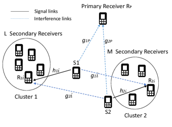
Figure 1: System model of co-existing underlay cognitive radio network

All channels are assumed to be independent, and of quasi-static Rayleigh fading type. The channels between $S_{1}$ and $R_{1i}$ are denoted by $h_{1i}\sim{\cal CN}\left(0,1/\lambda_{11}\right)$, $i\in[1,L]$. The channels between $S_{2}$ and $R_{2i}$ are denoted by $h_{2i}\sim{\cal CN}\left(0,1/\lambda_{22}\right)$, $i\in[1,M]$. Due to concurrent secondary transmissions, each transmitter interferes with the receivers of the other cluster. The interference channels between $S_{1}$ and $R_{2i}$ are denoted by $g_{1i}\sim{\cal CN}\left(0,1/\mu_{12}\right)$, $i\in[1,M]$, with $g_{1i^{*}}$ being the channel to the intended receiver $R_{2i^{*}}$. The interference channels between $S_{2}$ and $R_{1i}$ are denoted by $g_{2i}\sim{\cal CN}\left(0,1/\mu_{21}\right)$, $i\in[1,L]$, with $g_{2i^{*}}$ being the channel to the intended receiver $R_{1i^{*}}$. The channels to $R_{P}$ from $S_{1}$ and $S_{2}$ are denoted by $g_{1P}\sim{\cal CN}\left(0,1/\mu_{1P}\right)$ and $g_{2P}\sim{\cal CN}\left(0,1/\mu_{2P}\right)$ respectively. We neglect primary interference at the secondary nodes assuming the primary transmitter to be located far away from the secondary receivers, which is a common assumption in CR literature, and well justified on information theoretic grounds [11], [12]. Zero-mean additive white Gaussian noise of variance $\sigma_{n}^{2}$ is assumed at all terminals. As in all underlay networks, it is assumed that $S_{1}$ and $S_{2}$ can estimate $|g_{1P}|^{2}$ and $|g_{2P}|^{2}$ respectively by observing the primary reverse channel, or using pilots transmitted by $R_{P}$.

In every signaling interval, $S_{1}$ transmits unit energy symbols $x$ with power $P_{S1}=\alpha I_{P}/|g_{1P}|^{2}$ and $S_{2}$ transmits unit energy symbols $z$ with power $P_{S2}=(1-\alpha)I_{P}/|g_{2P}|^{2}$, where $I_{P}$ denotes the ITL, and $0<\alpha<1$ denotes the power allocation parameter which apportions $I_{P}$ between $S_{1}$ and $S_{2}$ respectively. We use peak interference type of power control at $S_{1}$ and $S_{2}$ instead of limiting the transmit powers with a peak power due to the following reasons:

1. It is well known that the performance of CR networks exhibits an outage floor after a certain peak power and does not improve beyond a point when transmit powers are limited by interference constraints.

2. Since sufficient peak power is typically available, this assumption is quite reasonable. It is in this regime where cognitive radios are expected to operate. Such an assumption is also common in prior underlay CR literature [13, 14, 15].

3. It keeps the analysis tractable, leading to precise performance expressions that offer useful insights. It also allows us to derive expressions for important parameters of practical interest in the normal range of operation of secondary networks, and can yield insights of interest to system designers.

The received signals ($y_{R_{1i}}$ and $y_{R_{2i}}$) at $R_{1i}$ and $R_{2i}$ can be written as follows:

$$y_{R_{1i}} = \sqrt{\frac{\alpha I_{P}}{|g_{1P}|^{2}}}h_{1i}x+\sqrt{\frac{(1-\alpha)I_{P}}{|g_{2P}|^{2}}}g_{2i}z+n_{R_{1i}},i\in[1,L]$$

$$y_{R_{2i}} = \sqrt{\frac{(1-\alpha)I_{P}}{|g_{2P}|^{2}}}h_{2i}z+\sqrt{\frac{\alpha I_{P}}{|g_{1P}|^{2}}}g_{1i}x+n_{R_{2i}},i\in[1,M],$$

where $n_{R_{1i}},n_{R_{2i}}\sim{\cal CN}(0,\sigma^{2}_{n})$ are additive white Gaussian noise samples at $R_{1i}$ and $R_{2i}$ respectively. When transmitters $S_{1}$ and $S_{2}$ select the receivers $R_{1i^{*}}$ and $R_{2i^{*}}$ with strongest link to them in their individual cluster, the instantaneous signal-to-interference-plus-noise ratios (SINRs) $\Gamma_{1}$ and $\Gamma_{2}$ at $R_{1i^{*}}$ and $R_{2i^{*}}$ can be written as follows:

$$\Gamma_{1} = \frac{\alpha I_{P}\frac{\displaystyle\max_{i\in[1,L]}{[|h_{1i}|^{2}]}}{|g_{1P}|^{2}}}{(1-\alpha)I_{P}\frac{|g_{2i^{*}}|^{2}}{|g_{2P}|^{2}}+\sigma_{n}^{2}}$$

$$\Gamma_{2} = \frac{(1-\alpha)I_{P}\frac{\displaystyle\max_{i\in[1,M]}{[|h_{2i}|^{2}]}}{|g_{2P}|^{2}}}{\alpha I_{P}\frac{|g_{1i^{*}}|^{2}}{|g_{1P}|^{2}}+\sigma_{n}^{2}}.$$ (2)

We note that the random variables $|h_{ij}|^{2}$ and $|g_{ij}|^{2}$ in (2) follow the exponential distribution with mean values $1/\lambda_{ii}$ and $1/\mu_{ij}$ respectively.

In the following section, we derive sum throughput expression for this co-existing secondary network. It gives a measure of spectrum utilization with or without concurrent transmissions by sources in co-existing secondary networks.

III Sum Throughput of the Secondary Network for Fixed Rate Transmission Scheme

When secondary nodes transmit with a fixed rate $R$, the sum throughput $\tau_{sum}$ is given by:

$$\tau_{sum} = (1-p_{out_{1}})R+(1-p_{out_{2}})R,$$ (3)

where $p_{out_{1}}$ and $p_{out_{2}}$ are outage probabilities of the two secondary user pairs $S_{1}$-$R_{1i^{*}}$ and $S_{2}$-$R_{2i^{*}}$ respectively.

III-A Derivation of $p_{out_{1}}$:

The outage probability $p_{out_{1}}$ is defined as follows:

$$p_{out_{1}} = \Pr\{\Gamma_{1}<\gamma_{th}\},$$

where $\gamma_{th}=2^{R}-1$. For notational convenience, we define random variable $X=\displaystyle\max_{i\in[1,L]}[|h_{1i}|^{2}]$. Clearly, it has cumulative distribution function (CDF) $F_{X}(x)=(1-e^{\lambda_{11}x})^{L}$. Thus, $p_{out_{1}}$ can be rewritten and evaluated as under:

$$p_{out_{1}} = \Pr\bigg{\{}X<\bigg{(}\frac{1-\alpha}{\alpha}\bigg{)}\gamma_{th}\frac{|g_{1P}|^{2}}{|g_{2P}|^{2}}|g_{2i^{*}}|^{2}+\frac{\gamma_{th}\sigma_{n}^{2}}{\alpha I_{P}}|g_{1P}|^{2}\bigg{\}}$$

$$= \mathbb{E}\bigg{[}\bigg{(}1-e^{-\lambda_{11}\{(\frac{1-\alpha}{\alpha})\gamma_{th}\frac{|g_{1P}|^{2}}{|g_{2P}|^{2}}|g_{2i^{*}}|^{2}+\frac{\gamma_{th}\sigma_{n}^{2}}{\alpha I_{P}}|g_{1P}|^{2}\}}\bigg{)}^{L}~{}\bigg{]}$$ (4)

$$= \mathbb{E}\bigg{[}1-\sum\limits_{j=1}^{L}\dbinom{L}{j}(-1)^{j+1}$$

$$\hskip 42.67912pte^{-\lambda_{11}j\{(\frac{1-\alpha}{\alpha})\gamma_{th}\frac{|g_{1P}|^{2}}{|g_{2P}|^{2}}|g_{2i^{*}}|^{2}+\frac{\gamma_{th}\sigma_{n}^{2}}{\alpha I_{P}}|g_{1P}|^{2}\}}\bigg{]},$$

where $\mathbb{E}[.]$ denotes the expectation over random variables $|g_{1P}|^{2}$, $|g_{2P}|^{2}$ and $|g_{2i^{*}}|^{2}$. We evaluate $p_{out_{1}}$ by successive averaging over random variables $|g_{2i^{*}}|^{2}$, $|g_{2P}|^{2}$ and $|g_{1P}|^{2}$ using standard integrals [16, eq.(3.353.5)] and [17, eq.(4.2.17)]. A final closed form expression for $p_{out_{1}}$ can be derived as follows (details omitted due to space limitations):

$$p_{out_{1}} = 1-\sum\limits_{j=1}^{L}\dbinom{L}{j}(-1)^{j+1}\bigg{[}\frac{1}{1+\frac{\lambda_{11}j\gamma_{th}\sigma_{n}^{2}}{\mu_{1P}\alpha I_{P}}}$$ (5)

$$-\frac{\frac{\mu_{2P}\lambda_{11}}{\mu_{1P}\mu_{21}}j(\frac{1-\alpha}{\alpha})\gamma_{th}\bigg{\{}\ln\bigg{(}\frac{1+\frac{\lambda_{11}j\gamma_{th}\sigma_{n}^{2}}{\mu_{1P}\alpha I_{P}}}{\frac{\mu_{2P}\lambda_{11}}{\mu_{1P}\mu_{21}}j(\frac{1-\alpha}{\alpha})\gamma_{th}}\bigg{)}}{[1+\frac{\lambda_{11}j\gamma_{th}\sigma_{n}^{2}}{\mu_{1P}\alpha I_{P}}-\frac{\mu_{2P}\lambda_{11}}{\mu_{1P}\mu_{21}}j(\frac{1-\alpha}{\alpha})\gamma_{th}]^{2}}$$

$$\hskip 43.36243pt+\bigg{(}\frac{\frac{\mu_{2P}\lambda_{11}}{\mu_{1P}\mu_{21}}j(\frac{1-\alpha}{\alpha})\gamma_{th}}{1+\frac{\lambda_{11}j\gamma_{th}\sigma_{n}^{2}}{\mu_{1P}\alpha I_{P}}}\bigg{)}-1\bigg{\}}\bigg{]}.$$

III-B Derivation of $p_{out_{2}}$:

The outage probability $p_{out_{2}}$ is defined as follows:

$$p_{out_{2}} = \Pr\{\Gamma_{2}<\gamma_{th}\}.$$ (6)

Due to the identical nature of SINR-s of $\Gamma_{1}$ and $\Gamma_{2}$, $p_{out_{2}}$ in (6) can be derived in the same manner as $p_{out_{1}}$, whose final closed form expression is shown as follows:

$$p_{out_{2}} = 1-\sum\limits_{k=1}^{M}\dbinom{M}{k}(-1)^{k+1}\bigg{[}\frac{1}{1+\frac{\lambda_{22}k\gamma_{th}\sigma_{n}^{2}}{\mu_{2P}(1-\alpha)I_{P}}}$$ (7)

$$-\frac{\frac{\mu_{1P}\lambda_{22}}{\mu_{2P}\mu_{12}}k(\frac{\alpha}{1-\alpha})\gamma_{th}\bigg{\{}\ln\bigg{(}\frac{1+\frac{\lambda_{22}k\gamma_{th}\sigma_{n}^{2}}{\mu_{2P}(1-\alpha)I_{P}}}{\frac{\mu_{1P}\lambda_{22}}{\mu_{2P}\mu_{12}}k(\frac{\alpha}{1-\alpha})\gamma_{th}}\bigg{)}}{[1+\frac{\lambda_{22}k\gamma_{th}\sigma_{n}^{2}}{\mu_{2P}(1-\alpha)I_{P}}-\frac{\mu_{1P}\lambda_{22}}{\mu_{2P}\mu_{12}}k(\frac{\alpha}{1-\alpha})\gamma_{th}]^{2}}$$

$$\hskip 43.36243pt+\bigg{(}\frac{\frac{\mu_{1P}\lambda_{22}}{\mu_{2P}\mu_{12}}k(\frac{\alpha}{1-\alpha})\gamma_{th}}{1+\frac{\lambda_{22}k\gamma_{th}\sigma_{n}^{2}}{\mu_{2P}(1-\alpha)I_{P}}}\bigg{)}-1\bigg{\}}\bigg{]}.$$

IV Optimal Power Allocation and Critical Target Rate

Our objective is to find the optimum $\alpha$ (denoted by $\alpha^{*}$) that maximizes $\tau_{sum}$. From (3), it is clear that $\alpha^{*}=\arg\displaystyle\max_{\alpha}(\tau_{sum})$. In normal mode of operation, the interference channel variances are small ($\mu_{1P}$ and $\mu_{2P}$ are large) so that $\lambda_{11}<<\mu_{1P}I_{P}$ and $\lambda_{22}<<\mu_{2P}I_{P}$. Hence, the terms $\frac{\lambda_{11}j\gamma_{th}\sigma_{n}^{2}}{\mu_{1P}\alpha I_{P}}$ and $\frac{\lambda_{22}k\gamma_{th}\sigma_{n}^{2}}{\mu_{2P}(1-\alpha)I_{P}}$ in (5) and (7) respectively are small quantities for practical values of target rates and can be ignored. (Computing $\alpha^{*}$ for high target rates is not required, as would become apparent in subsequent discussions.) Thus $p_{out_{1}}$ and $p_{out_{2}}$ reduce to the following form with $x=\frac{\mu_{2P}\lambda_{11}}{\mu_{1P}\mu_{21}}(\frac{1-\alpha}{\alpha})$ and $y=\frac{\mu_{1P}\lambda_{22}}{\mu_{2P}\mu_{12}}(\frac{\alpha}{1-\alpha})$:

$$p_{out_{1}} \approx \sum\limits_{j=1}^{L}\dbinom{L}{j}(-1)^{j+1}\gamma_{th}xj\frac{(\gamma_{th}xj-\ln(\gamma_{th}xj)-1)}{(1-\gamma_{th}xj)^{2}},$$

$$p_{out_{2}}\approx\sum\limits_{k=1}^{M}\dbinom{M}{k}(-1)^{k+1}\gamma_{th}yk\frac{(\gamma_{th}yk-\ln(\gamma_{th}yk)-1)}{(1-\gamma_{th}yk)^{2}}.$$

Using the first order rational approximation for logarithm [18] $\ln(z)\approx\frac{2(z-1)}{(z+1)}$ in (LABEL:eq:_IP_approx_asymptote), which is close to (or follows) the logarithm function for a large range of $z$ (and also used in underlay literature [15]), $z\frac{(z-\ln(z)-1)}{(1-z)^{2}}\approx\frac{z}{z+1}$. Hence, $p_{out_{i}},i\in\{1,2\}$ in (LABEL:eq:_IP_approx_asymptote) can further be approximated as:

$$p_{out_{1}} \approx 1-\sum\limits_{j=1}^{L}\dbinom{L}{j}(-1)^{j+1}\frac{1}{\gamma_{th}xj+1},$$ (9)

$$p_{out_{2}}\approx 1-\sum\limits_{k=1}^{M}\dbinom{M}{k}(-1)^{k+1}\frac{1}{\gamma_{th}yk+1}.$$

Obtaining $\alpha^{*}$ for general $L$ and $M$ is mathematically tedious, and can be evaluated offline by numerical search. However, we present a closed form $\alpha^{*}$ for the special case when $L=M=1$. By taking the first derivative of $\tau_{sum}$ with respect to $\alpha$ using $p_{out_{1}}$ and $p_{out_{2}}$ in (9), and equating it to zero, a closed form $\alpha^{*}$ can be obtained with the root in [0,1] being:

$$\alpha^{*} \approx \frac{1}{1+\frac{\mu_{1P}}{\mu_{2P}}\sqrt{\frac{\lambda_{22}}{\lambda_{11}}\frac{\mu_{21}}{\mu_{12}}}}.$$ (10)

By taking the second derivative of $\tau_{sum}$ with respect to $\alpha$, and upon substitution of $\alpha^{*}$ from (10), an expression is obtained, which can either be positive or negative depending on the value of $\gamma_{th}$ (details are omitted due to space constraints). By equating the expression to zero and solving for $\gamma_{th}$ (or equivalently for $R$), a closed form expression of critical target rate $R=R_{c}$ (for $L=M=1$) can be obtained³ as:

$$R_{c} \approx \log_{2}\bigg{(}1+\sqrt{\frac{\mu_{12}\mu_{21}}{\lambda_{11}\lambda_{22}}}\bigg{)}.$$ (11)

When $R<R_{c}$, $\tau_{sum}$ is concave with respect to $\alpha$ and concurrent transmission offers higher throughput. When $R>R_{c}$, switching to single secondary transmission is optimal, as $\tau_{sum}$ is convex with respect to $\alpha$. For a generalized $L$ and $M$ users, $R_{c}$ and $\alpha^{*}$ can be evaluated by an offline numerical search².

For larger $L$ and $M$ (multiple secondary users in each network), when a round robin scheduling scheme is used, the channel characteristics are exponential (same as when $L=M=1$), and (10) and (11) are valid for $\alpha^{*}$ and $R_{c}$. We emphasize that $R_{c}$ and $\alpha^{*}$ both depend only on statistical channel parameters and do not require real-time computation.

V Simulation Results

In this section, we present simulation results to validate the derived expressions and bring out useful insights. We assume $\mathbb{E}[|h_{ij}|^{2}]\propto d_{ii}^{-\phi}$, $d_{ii}$ being the normalized distance between the transmitter and intended receiver in cluster $i$, where $i\in\{1,2\}$ and $j\in\{L,M\}$. Again, $\mathbb{E}[|g_{ij}|^{2}]\propto r_{ij}^{-\phi}$ is assumed, where $r_{ij}$ is the normalized distance between the transmitter of cluster $i$ to the receiver of cluster $j$, where, $i\in\{1,2\}$ and $j\in\{L,M,P\}$. The pass-loss exponent is denoted by $\phi$ (assumed to be $3$ in this paper).

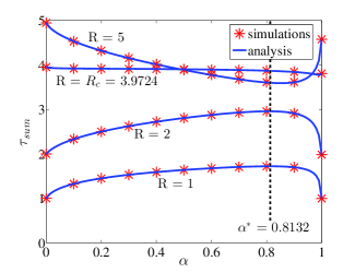
Figure 2: $\tau_{sum}$ vs $\alpha$ for $R=1,2,R_{c},5$.

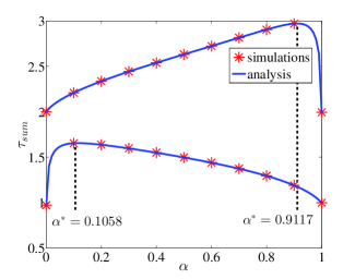
Figure 3: $\tau_{sum}$ vs $\alpha$ with optimum power allocation for different channel parameters, target rates and ITL

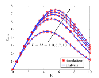
Figure 4: $\tau_{sum}$ vs $R$ with $L=M=1,3,5,7,10$.

In Fig. 2 we plot $\tau_{sum}$ vs $\alpha$ for different target rates. The system parameters chosen are as follows: $d_{11}=2$ units, $d_{22}=1$ unit, $r_{1P}=r_{2P}=3$ units, $r_{12}=4$ units, $r_{21}=3$ units. $L=M=1$ and $I_{P}=20dB$ is assumed. When target rates are below $R_{c}=3.9724$ (as calculated from (11)), there is an improvement in sum throughput of the order of $1$ bpcu when optimum $\alpha$ is chosen using concurrent transmission. If $R$ exceeds $R_{c}$, switching to single secondary network is best. This happens because with high target rates, both user pairs suffer link outages, and mutual interferences further degrades performance. Switching to a single network not only improves transmit power, but also nullifies the interference from the other network, which cumulatively improve outage and throughput performance.

In Fig. 3 we plot $\tau_{sum}$ vs $\alpha$ assuming $L=M=1$ for varying channel parameters, target rates and ITL to show that $\alpha^{*}$ as evaluated in (10) gives a fairly accurate and robust measure of optimal ITL apportioning between $S_{1}$ and $S_{2}$, and improves sum throughput performance. The system parameters chosen for the first plot are as follows: $d_{11}=1$ unit, $d_{22}=2$ units, $r_{1P}=4$ units, $r_{2P}=3$ units, $r_{12}=3$ units, $r_{21}=3.5$ units and $I_{P}$ is chosen as $10dB$. $R=1$ is assumed to ensure that $R<R_{c}=3.7037$ (so that concurrent transmission is advantageous). $\alpha^{*}=0.1058$ is obtained from (10). In the second plot, we assume the following parameters: $d_{11}=2$ unit, $d_{22}=1$ units, $r_{1P}=3$ units, $r_{2P}=4$ units, $r_{12}=4$ units, $r_{21}=3$ units and $I_{P}$ is chosen as $25dB$. $R=2$ is assumed to ensure that $R<R_{c}=3.9724$ (so that concurrent transmission is advantageous). $\alpha^{*}=0.9117$ is obtained from (10). We note, for symmetric channel conditions, $ie$ $\lambda_{11}=\lambda_{22}$, $\mu_{12}=\mu_{21}$ and $\mu_{1P}=\mu_{2P}$, $\alpha^{*}=0.5$, implying equal resource allocation between $S_{1}$ and $S_{2}$. In addition we have the following observations: 1) $\alpha$ decreases when the ratio $\frac{\mu_{1P}}{\mu_{2P}}$ increases, or when $S_{2}$ is closer to the primary than $S_{1}$. This implies throughput can be maximized if more power is allocated to $S_{2}$ (thereby improving its outage), as $S_{1}$ has a weaker channel to primary (has more available power) and can meet its outage requirement with less transmit power. 2) $\alpha$ decreases with increase in $\frac{\lambda_{22}}{\lambda_{11}}$. In other words, when $S_{1}$-$R_{1i^{*}}$ channel is better than $S_{2}$-$R_{2i^{*}}$, $S_{1}$ is able to meet its outage requirement with less power, and more power needs to be allocated to $S_{2}$ to improve performance. 3) $\alpha$ decreases with the ratio $\frac{\mu_{21}}{\mu_{12}}$, or when the channel between $S_{1}$ to $R_{2i^{*}}$ is better than the channel between $S_{2}$ to $R_{1i^{*}}$. Thus, allocating more power to $S_{2}$ causes less interference to users of $S_{1}$, which improves the overall throughput.

In Fig. 4, we plot $\tau_{sum}$ in (3) vs $R$ and show the effect of number of users in the two networks on sum throughput performance with concurrent transmissions. We choose parameters as follows: $d_{11}=d_{22}=1$ unit, $r_{1P}=r_{2P}=3$ units and $r_{12}=r_{21}=3$ units. $\alpha=0.5$ and $I_{P}=20dB$ is chosen. Clearly, $\tau_{sum}$ increases with $L$ and $M$. From (11), it is also clear that $R_{c}$ increases with user selection (this $R_{c}$ refers to a network having generalized $L$ and $M$ users, which is not derived in this paper. However, intuitively it is clear that user selection statistically improves the main channels, thereby increasing $R_{c}$ as in (11)), which causes a rightward shift of the peaks of $\tau_{sum}$. As also evident from earlier discussions, $\tau_{sum}$ first increases and then decreases after a certain critical rate as both $S_{1}$-$R_{1i^{*}}$ and $S_{2}$-$R_{2i^{*}}$ links start to suffer from outages, thereby decreasing the overall throughput performance with concurrent transmissions.

VI Conclusion

In this paper we analyze the sum throughput performance of two co-existing underlay multiuser secondary downlink networks utilizing fixed-rate transmissions. In the single user scenario, or in a multiuser scenario without opportunistic user selection, we establish that there exists a fixed critical rate beyond which co-existing secondary networks results in lower throughput. During concurrent secondary transmissions, we establish that user selection as well as judicious interference temperature apportioning, can increase throughput performance.

VII Acknowledgment

This work was supported by Information Technology Research Academy through sponsored project ITRA/15(63)/Mobile/MBSSCRN/01. The authors thank Dr. Chinmoy Kundu for his inputs on this work.

References

- [1] L. B. Le and E. Hossain, “Resource allocation for spectrum underlay in cognitive radio networks,” IEEE Trans. Wireless Commun., vol. 7, no. 12, pp. 5306–5315, Dec. 2008.
- [2] J. Lee, H. Wang, J. G. Andrews, and D. Hong, “Outage probability of cognitive relay networks with interference constraints,” IEEE Trans. Wireless Commun., vol. 10, no. 2, pp. 390–395, Feb 2011.
- [3] P. L. Yeoh, M. Elkashlan, K. J. Kim, T. Q. Duong, and G. K. Karagiannidis, “Transmit antenna selection in cognitive MIMO relaying with multiple primary transceivers,” IEEE Trans. Veh. Technol., vol. 65, no. 1, pp. 483–489, Jan 2016.
- [4] J. V. Hecke, P. D. Fiorentino, V. Lottici, F. Giannetti, L. Vandendorpe, and M. Moeneclaey, “Distributed dynamic resource allocation for cooperative cognitive radio networks with multi-antenna relay selection,” IEEE Trans. Wireless Commun., vol. 16, no. 2, pp. 1236–1249, Feb 2017.
- [5] H. K. Boddapati, M. R. Bhatnagar, and S. Prakriya, “Ad-hoc relay selection protocols for multi-hop underlay cognitive radio networks,” in 2016 IEEE GC Wkshps, Dec 2016, pp. 1–6.
- [6] S. M. Cheng, W. C. Ao, F. M. Tseng, and K. C. Chen, “Design and analysis of downlink spectrum sharing in two-tier cognitive femto networks,” IEEE Trans. Veh. Technol, vol. 61, no. 5, pp. 2194–2207, Jun 2012.
- [7] S. M. Cheng, S. Y. Lien, F. S. Chu, and K. C. Chen, “On exploiting cognitive radio to mitigate interference in macro/femto heterogeneous networks,” IEEE Wireless Commun., vol. 18, no. 3, pp. 40–47, Jun 2011.
- [8] M. Peng, C. Wang, J. Li, H. Xiang, and V. Lau, “Recent advances in underlay heterogeneous networks: Interference control, resource allocation, and self-organization,” IEEE Commun. Surveys Tuts., vol. 17, no. 2, pp. 700–729, Secondquarter 2015.
- [9] Y. Xing, C. N. Mathur, M. A. Haleem, R. Chandramouli, and K. P. Subbalakshmi, “Dynamic spectrum access with QoS and interference temperature constraints,” IEEE Trans. Mobile Comput., vol. 6, no. 4, pp. 423–433, Apr 2007.
- [10] X. Kang, R. Zhang, and M. Motani, “Price-based resource allocation for spectrum-sharing femtocell networks: A stackelberg game approach,” IEEE J. Sel. Areas Commun., vol. 30, no. 3, pp. 538–549, Apr 2012.
- [11] A. Jovicic and P. Viswanath, “Cognitive radio: An information-theoretic perspective,” IEEE Trans. Inf. Theory, vol. 55, no. 9, pp. 3945–3958, Sep. 2009.
- [12] M. Vu, N. Devroye, and V. Tarokh, “On the primary exclusive region of cognitive networks,” IEEE Trans. Wireless Commun., vol. 8, no. 7, pp. 3380–3385, Jul. 2009.
- [13] T. Q. Duong, D. B. da Costa, M. Elkashlan, and V. N. Q. Bao, “Cognitive amplify-and-forward relay networks over Nakagami-m fading,” IEEE Trans. Veh. Technol., vol. 61, no. 5, pp. 2368–2374, Jun 2012.
- [14] K. Tourki, K. Qaraqe, and M.-S. Alouini, “Outage analysis for underlay cognitive networks using incremental regenerative relaying,” IEEE Trans. Veh. Technol., vol. 62, no. 2, pp. 721–734, Feb. 2013.
- [15] P. Chakraborty and S. Prakriya, “Secrecy outage performance of a cooperative cognitive relay network,” IEEE Commun. Lett., vol. 21, no. 2, pp. 326–329, Feb 2017.
- [16] I. S. Gradshteyn and I. M. Ryzhik, Table of integrals, series, and products, 7th ed. Academic, 2007.
- [17] M. Geller and E. W. Ng, “A table of integrals of the exponential integral,” J. Res. Nat. Bureau Std., vol. 73B, no. 3, pp. 191–210, Sep. 1969.
- [18] F. Topsøe, “Some bounds for the logarithmic function,” RGMIA Res. Rep. Collection, vol. 7, no. 2, 2004.