Non-energy-eigenbasis measurements on an ultra-strongly-coupled system interacting with a driven nonlinear resonator
Abstract
We explore the problem of projecting the ground state of a system into a superposition between energy eigenstates when the coupling between measurement device and system is much smaller than the energy scales of the system itself. As a specific example, we investigate an ultra-strongly coupled light-matter system whose ground state exhibits non-trivial entanglement between the atom and photons. As a measurement apparatus we consider both linear and non-linear driven resonators. We find that the state of the non-linear resonator can exhibit a much stronger correlation with the ultra-strongly coupled system than the linear resonator, even when the system-measurement apparatus coupling strength is weak. Also, we investigate the conditions for when the nonlinear resonator can be entangled with the ultra-strongly coupled system, which allows us to project the ground state of the ultra-strongly coupled system into a non-energy eigenstate. Our proposal paves the way to realize projective measurements in an arbitrary basis, which would significantly broaden the possibilities of controlling quantum devices.
A quantum measurement typically projects the a system into an eigenstate of the measured observable . In quantum measurement theory, the measurement apparatus interacts with the target system due to an interaction Hamiltonian , where denotes the operator of the apparatus and denotes a coupling strength measurement1 ; qndcondition . This process induces a correlation between the system and apparatus. A subsequent measurement on the apparatus itself implements the projection of the target system, and the readout of the apparatus is associated with the eigenvalues of the system observable . To realize a quantum non-demolition measurement, the observable should commute with the target system Hamiltonian qndcondition . In addition, in several experiments measurement3 ; jba2 ; jba3 ; jba4 , projective measurements on quantum systems have been demonstrated directly in the energy-eigenbasis itself, where the observable is the Hamiltonian of the target system.
Although projective measurements in an arbitrary basis would significantly broaden the possibilities of controlling quantum states if realized application1 ; application2 ; application3 , such non-energy-eigenbasis measurements are, surprisingly, sometimes not straightforward. Ideally, if the system observable to be measured does not commute with the system Hamiltonian, has a matrix component to induce transitions between the energy eigenstates. Importantly, however, if the coupling strength is much smaller than the energy of the system, such transition matrix components disappear under a rotating wave approximation introductory (see Appendix A for details), and we cannot project the system into the eigenbasis of ; the system stays in its energy eigenbasis.
On the other hand, if the coupling between the system and apparatus is much larger than the system energy, one can perform a projective measurement much faster than the typical time scale of the system, hence realizing non-energy eigenbasis measurements ashhab ; ashhab2 ; ashhab3 . However, if energy scales are comparable, the dynamics, and the subsequent quantum measurement process, becomes much more complicated than the cases described above. Understanding the interaction between the apparatus and system, and their dynamics, is important not only for explaining the mechanism of quantum projective measurements but also to achieve a higher level of control over quantum states.
The ultra-strong and deep-strong coupling regimes between atoms and light is an especially attractive area to explore the possibility of non-energy eigenbasis measurements. This is because the ground state of this system exhibits non-trivial entanglement between the atom and photons, and virtual excitations, which are difficult to probe with energy eigenbasis measurements alone. This hybridization of light and matter is one of the core topics in quantum physics hybrid1 ; hybrid2 ; hybrid3 ; bulute11 ; georgescu12 ; hybrid4 ; hybrid5 ; XinWang ; ultra12 . In addition, when the coupling strength between light and matter becomes extremely strong, so that it surpasses the cavity resonance frequency, it is predicted that a new ground state will emerge ultra1 ; ultra2 ; ultra3 ; ultra4 ; protected ; roberto2017 ; transition ; felicett ; u8 ; u9 ; u10 ; u11 ; u12 ; u13 ; u14 ; u15 ; u16 ; u17 . Such a regime was recently experimentally demonstrated expultra1 ; expultra2 ; expultra3 .
Measurements of ultra-strongly-coupled systems so far have mostly focused on extraction of photons from the ground state, via modulation of some system parameter Simone ; christian (akin to approaches used to observe the dynamical Casimir effect dcasimir3 ; dcasimir2 ; dcasimir1 ; dcasimir4 ; dcasimir5 ), or transitions out of the ground-state itself Roberto ; Mauro_dqd . In addition, another proposal suggested using an ancillary qubit coupled to an ultra-strongly coupled system Ciuti , with the goal of doing QND measurement of the photons in the ground state. Since the ground state of the ultra-strongly-coupled system contains virtual photons, we can also in principle extract the virtual photons if the state is projected into a non-energy eigenbasis state Simone (akin to approaches used to observe the dynamical Casimir effect dcasimir3 ; dcasimir2 ; dcasimir1 ; dcasimir4 ; dcasimir5 ).
If we could observe such photons extracted from the ground state, this would be a direct evidence of the implementation of the non-energy eigenbasis states. Moreover, non-eigenbasis measurements on a ground state of a ultra-strongly-coupled system could potentially be used to induce an optical cat state, which is itself a resource for quantum information processing protected ; roberto2017 . Given these potential benefits, and open problems to be solved, the ultra-strongly-coupled system is attractive as an example with which to investigate the problem of non-energy eigenbasis measurements. Although there are several previous works studying the quantum properties of the ground state in an ultra-strongly-coupled system Ciuti ; Mauro ; ultra1 ; ultra2 ; ultra3 ; ultra4 , here we focus only on how to perform non-energy eigenbasis measurements on the ground state of such a system.
In this paper, we specifically analyze the dynamics of an ultra-strongly coupled system interacting with a measurement apparatus, when the measured system observable does not commute with the system Hamiltonian. We evaluate the dynamics of the measurement apparatus during the interaction, the back-action of the measurements on the system, and the correlations between the system and the apparatus. Such properties are typically studied when one tries to examine in detail a quantum measurement process nakano ; trajectory ; backaction ; continuous . Although there exist theoretical proposals to use a detector that continuously monitors the system ashhab2 , here we consider a binary-outcome measurement performed on the measurement apparatus after the measurement apparatus and system have been allowed to interact. Such a binary-outcome measurement is understood to induce a strong correlation with the system jba6 ; kakuyanagijps , which is crucial to realize our goal of non-energy eigenbasis measurements.
While linear resonators are used as a standard method for quantum measurement in cavity quantum electrodynamics and circuit quantum electrodynamics, in some cases a nonlinearity has been employed to improve qubit readout jba1 ; jba2 ; jba3 ; jba4 ; jba5 ; jba6 . Due to the bifurcation effect, the state of the nonlinear resonator becomes highly sensitive to the state of the system, which enables one to implement a high-visibility readout. Here, with both full numerical modeling and a low-energy approximation, we investigate how such a driven nonlinear resonator interacts with the ultra-strongly-coupled system. Surprisingly, although the coupling between the nonlinear measurement device and the ultra-strongly-coupled system is weak compared to system energy scales, we show that the dynamic evolution can induce a strong correlation between them, which shows that the non-linear resonator would be a suitable device to realize the non-energy eigenbasis measurements. Moreover, we evaluate how much quantum correlations such as entanglement and quantum discord are generated between system and measurement device during this evolution. These results let us know the conditions when the non-energy eigenbasis measurements can be realized with this system.
The remainder of this paper is organized as follows. First, we introduce the ultra-strongly-coupled system and its ground state. Second, we discuss the interaction between the nonlinear resonator and the ultra-strongly-coupled system, and we introduce a coarse-graining measurement of the nonlinear resonator itself. Third, we present numerical results to show how a strong correlation arises, even in a parameter regime where the coupling strength may be incorrectly considered to be negligible. Fourth, we show that, as the effective energy of the ultra-strongly-coupled system decreases, the entanglement between the ultra-strongly coupled system and the nonlinear resonator-increases. Finally, we examine the quantum discord between the ultra-strongly coupled system and the nonlinear resonator.
I Ultra-strong coupling between light and matter
The Hamiltonian of light in a single-mode cavity ultra-strongly-coupled to matter (where the matter is well described by a two-level system) is, in its simplest form, given by the Rabi model rabi
| (1) |
where () is an annihilation (creation) operator for the single-mode cavity/resonator, () denotes the qubit (resonator) frequency, and is the coupling strength between resonator (light) and qubit (matter).
Recall that, when the matter is in the form of a superconducting flux qubit, as in the recent ultra-strong coupling experiments in expultra1 ; expultra2 ; expultra3 , is diagonal in the persistent-current basis of and of the superconducting flux qubit.
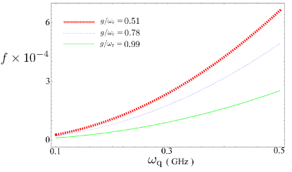
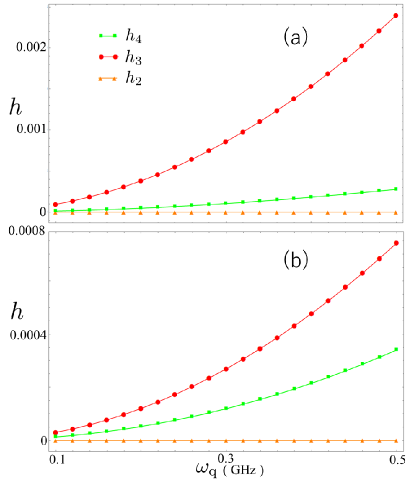
Throughout this paper we assume that the qubit frequency is much smaller than the resonator frequency, allowing us later to use an adiabatic approximation. In this case, in the limit , we can approximately write the ground state of this system as ultra1
| (2) |
where
| (3) |
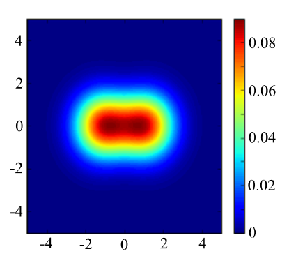
is the ratio of the coupling strength and resonator energy. As an example, using parameters close to those used in expultra1 , we plot the function of the reduced density matrix of where the atom is traced out in Fig.1. The definition of the function for a state is , where is a coherent state for a complex number . We plot the real part of the in the axis while we plot the imaginary part of the in the axis. It is worth mentioning that, if we can realize a projective measurement in the basis of or on this ground state, we can create an optical cat state, , in the cavity.
II Using a nonlinear resonator as a measurement device
Here, as a measurement apparatus, we consider a driven nonlinear resonator dispersively coupled to the qubit. It is well understood that a nonlinear resonator can exhibit a bistability rigo ; nakano ; clerk1 ; clerk2 ; backaction , which makes such a device sensitive to small changes in external fields. In addition, the nonlinearity induces a rapid change in the photon number under driving nakano , compared to the linear case. When used as a measurement device, the fast evolution and the sensitivity of the steady-state to weak fields results in a strong and fast correlation of the nonlinear resonator state with the qubit being measured, potentially giving a means to implement a rapid projective measurement. One should note that typically the state of the nonlinear resonator is itself measured by standard homodyne techniques rabi , and this measurement provides the information about the qubit state.
It is worth mentioning that there are some theoretical proposals to treat such a measurement device as a two level system when the measurement outcomes are binary ashhab . However, since such a simplification cannot quantify the strength of the correlation between the target qubit and measurement apparatus during the measurement process, we need to model the measurement apparatus with a proper Hamiltonian as we will describe below.
The total system, composed of the ultra-strongly-coupled light-matter system, and the nonlinear resonator measurement device, can be described by the Hamiltonian in the laboratory frame ultra1 ; ultra3 ; ultra4 ; nakano ; clerk1 ; clerk2 ; backaction
| (4) | ||||
| (5) | ||||
| (6) |
where is an annihilation operator of the nonlinear system, denotes the detuning between the nonlinear resonator energy and driving frequency, is the nonlinearity strength, denotes the driving strength of the nonlinear resonator, and is the driving frequency of the nonlinear resonator. In addition, is the coupling between the qubit and the nonlinear resonator, which is not derived from the dispersive approximation to a dipole coupling, but is intrinsic (see Appendix B for details.) In the rotating frame defined by and by applying the rotating wave approximation, we have
| (7) | ||||
| (8) | ||||
| (9) |
In order to include the loss of photons from the nonlinear resonator, we adopt the following Lindblad master equation, valid when the coupling between nonlinear resonator and its environment is weak, and when the coupling between nonlinear resonator and qubit is weak nakano ; clerk1 ; clerk2 ; backaction
| (10) |
where denotes the photon leakage rate from the nonlinear cavity. The potential losses from the ultra-strongly coupling system are described later.
II.1 Coarse-graining of the measurement outcome
After the qubit and the measurement apparatus have interacted for some time, we need to implement a measurement on the measurement apparatus itself. Ideally, one could apply a projection operator on the nonlinear resonator, where is an eigenvector of the quadrature operator . However, due to imperfections in the measurement setup, one cannot resolve arbitrarily small differences in the state of the resonator. Normally, to describe more realistically the measurement process, one takes this into account by considering the integrated signal-to-noise bathinte , where the noise can include contributions from vacuum fluctuations and noise in the measurement apparatus itself. Here, instead we employ a “coarse graining” approximation described by the following operator
| (11) |
where is the width of the error of the measurement process, and the post-measurement state is described by . Similar coarse graining approaches have been made in Refs. coarse1 ; coarse2 . This approach allows us to consider the transition from small to large noise situations without being specific about the source of the noise.
Correlations between the nonlinear resonator and the qubit should occur after they have interacted for some time, and, for the parameter regime we use in this work, typically the nonlinear resonator state with () corresponds to an outcome where the qubit was initially in its excited (ground) state. We can describe the post measurement state of the ultra-strongly-coupled (USC) system as (see Appendix C for details)
| (12) | ||||
| (13) |
where is the complementary error function and and are normalization factors.
In the limit when , we obtain . In this case, the measurement results do not contain any information of the post-measurement state of the qubit. On the other hand, we obtain
| (14) |
and
| (15) |
in the limit , which corresponds to an ideal projective measurement that can perfectly distinguish or .
II.2 Losses in ultra-strongly coupled systems
We must also consider the coupling between the cavity component of the ultra-strongly-coupled system and its environment. This allows us to evaluate properties of the photons leaking out from the system after the measurement on the nonlinear resonator. The interaction Hamiltonian between the system and the environment can be described as bathinte
| (16) |
where denotes a boson annihilation operator for the environment (e.g., an open transmission line). When we move to the Heisenberg picture, defined by the Hamiltonian , the operator becomes time dependent. We can define , where () denotes the positive (negative) frequency component xoperator1 ; xoperator2 ; xoperator3 . With a rotating wave approximation, we have
| (17) |
By using a Markov approximation with the standard input-output formalism bathinte , we obtain
| (18) | ||||
| (19) |
where () denotes an output (input) operator. This means that the photons leaking from the USC system into the transmission line are described by the operators and . We use these definitions to describe the potentially observable real photons in the USC system. However, in the simulations we perform, we assume that the decay time of the USC system is longer than all other time scales that we consider, and so we only explicitly take into account the decay of the nonlinear measurement apparatus.
III Full dynamics of the USC system and nonlinear measurement device
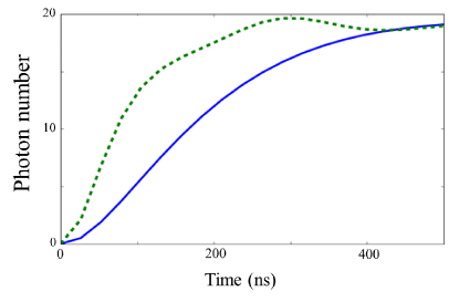
Using the parameters from expultra1 , we numerically qutip ; qutip2 solve Eq. (10), with the USC system in the initial state , and we consider the post-measurement state of the USC system after the coarse-graining measurement on the nonlinear resonator is performed at the time . In Fig. 2, we show how the function of the resonator part of the USC system depends on the coarse-graining value. One immediately sees a change in the state of the USC resonator when the measurement becomes weaker (corresponding to an increase of the coarse-graining values of ).
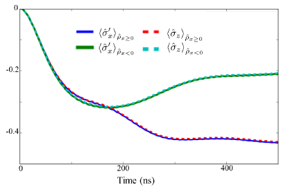
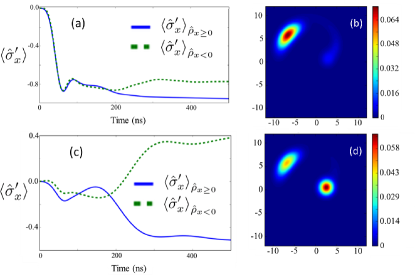
In Figs. 3 and 4 we plot the post-measurement observable photons in the USC cavity, and the state of the qubit , for and . For comparison, we consider both a linear resonator () and a nonlinear resonator () as the measurement devices. In addition, in Fig. 5, we show the average photon number inside the measurement resonator, also for the case of a nonlinear and a linear device. In all figures, for the nonlinear measurement resonator, when we set the coarse-graining value as , the post-measurement state of the USC cavity and qubit changes significantly, depending on the measurement outcome, and so we observe a clear measurement backaction on the ultra-strongly coupled system. Interestingly, in these examples, we set the coupling strength as approximately times smaller than the qubit energy. On the other hand, for a linear resonator, the effect of the measurement backaction is negligible in this regime, and the post-measurement state is almost independent of the measurement results.
III.1 Low-energy two-level approximation
To give an intuitive explanation for why the nonlinear resonator measurement apparatus can become strongly correlated with the USC system, even when the coupling between measurement apparatus and system is much smaller than the system energy scales, we introduce a two-level approximation for the USC system. (see Appendix D for details, and a detailed analysis of the validity of this approximation). In our simulations, the initial state is , and the interaction Hamiltonian mainly induces a transition from to the first excited state . Since the transition matrix elements of the interaction Hamiltonian to the other excited states are negligible, we can approximate the low-energy states of the ultra-strongly-coupled system as a two-level system. In this case, and can be written as
| (20) | ||||
| (21) |
where
| (22) |
and
| (23) | ||||
| (24) |
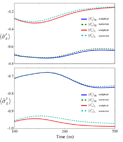
In Fig. 6, we plot corresponding to and , with this two-level system approximation. To check the validity of this simplified model, we plot with this model and using the full model in Fig. 6. These results show an excellent agreement.
With this two-level approximation, we can show that the large correlation between the nonlinear resonator and the ultra-strongly-coupled system originates from the combination of an AC Stark shift and an adiabatic transition. It is easy to see that the large number of photons in the nonlinear resonator induces an energy shift (AC Stark shift) of the USC two-level system. Since the photon number of the high-amplitude state is different from that of the low-amplitude state, the size of the AC Stark shift strongly depends on the state of the nonlinear resonator. As long as the timescale of the change in the nonlinear resonator photons is much smaller than , the state of the two-level system remains in a ground state of the following effective Hamiltonian
| (25) |
where () is the average photon number of the high (low) amplitude state.
When the nonlinear measurement resonator becomes a mixed state of the low- and high-amplitude states, we expect that the AC Stark shift (whose amplitude depends on the nonlinear resonator state) induces an adiabatic change of the ground state of the two-level system. This leads to a large correlation between the USC system and the measurement resonator. To show the validity of this interpretation, we analytically calculate the of the ground state of the Hamiltonian in Eq. (25) where we substitute the numerically calculated photon numbers of the high (low) amplitude state for (). In Fig. 7, we compare these results with the numerical simulations qutip ; qutip2 where the master equation with the simplified Hamiltonian is solved. There is a good agreement between these two results, leading us to conclude that the correlation between the two-level system and the nonlinear resonator is induced by the aforementioned adiabatic changes due to the AC Stark shift, whose amplitude depends on the nonlinear resonator state. Note that in Fig. 7 we do not show the time evolution from to , because the high-amplitude state is not generated until approximately .
III.2 Comparison to QND limit
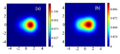
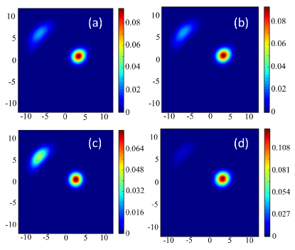
To compare our non-energy eigenbasis measurements with a ideal quantum non-demoliton (QND) measurements, we now study the behavior of the the function of the nonlinear resonator, as shown in Fig. 8. Here, we consider the following four cases: (a) a non-energy eigenbasis measurement with the full Hamiltonian described in Eq. (7), (b) a non-energy eigenbasis measurement with the two-level system approximation described by Eq. (25), (c) quantum non-demoliton measurements for the full Hamiltonian described in Eq. (7) for the limit (which makes the measurement satisfy the QND condition ), and (d) null measurements with .
First, we again confirm that the two-level approximation (b) compares well to the full Hamiltonian case (a). Moreover, we observe a clear difference between our non-energy eigenbasis measurements and measurements in the QND limit (c). In particular, the probability to obtain the high-amplitude state in the the nonlinear resonator becomes much larger for QND measurements than that for the the non-energy eigenbasis measurement case.
Second, a naive application of the rotating-wave approximation to the system and measurement device coupling term, for the non-energy eigenbasis measurement case, suggests that the influence of system and measurement apparatus on each other should be entirely negligible. Of course, there is a clear difference between the case with a finite and the case without , because such an approximation should also take into account the norm of the operator in the interaction term, which for the driven nonlinear resonator can be large. The figures show that, roughly speaking, the probability to obtain the high-amplitude state of the resonator for the non-energy eigenbasis measurements lies between the case of the QND measurements and null measurements.
Also, we increase the ratio to check how the effect of the AC Stark shift will change. In Fig. 9(a), we plot , , and the function at where the effective energy is % that used in Fig.4. From Fig. 9(a), the system converges into an eigenstate of after the interaction, regardless of the measurement results of the nonlinear resonator. This can be understood by considering that the AC Stark effect becomes much larger than the effective energy so that the state of the ultra-strongly-coupled system becomes an eigenstate of for both the high amplitude state and low amplitude state. Furthermore, it is worth mentioning that, from Fig. 9(b), the nonlinear resonator before the measurement almost becomes a high-amplitude state. For an ideal quantum projective measurements on the ground state of the ultra-strongly coupled system, the population in the low-amplitude state should be the same as that of the high-amplitude state, and so this result shows that the effective energy is still too large to realize a full projective measurement in the persistent current basis.
We also consider a case when the effective energy is % of that used in Fig. 4. In that case, becomes much larger than , and this cannot be explained just by the AC Stark shift. Moreover, from Fig. 9(c), the population of the high-amplitude state becomes comparable with that of the low-amplitude state. Therefore, in this regime, we realize a strong projection of the ground state of the ultra-strongly-coupled system in the non-energy eigenbasis.
IV Negativity
As a criteria of entanglement, and to understand how correlations between nonlinear resonator and USC system develop, we consider the negativity. Suppose there is a Hilbert space of two systems, with a state . The definition of negativity is
| (26) |
here, is the partial transpose of the state taken over a subsystem , and is the trace norm negativity1 . In our case, the subsystem corresponds to the two-level system approximation of the USC system, and to the nonlinear resonator.
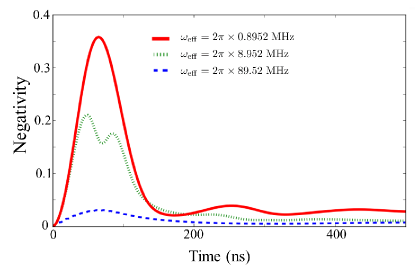
In Fig. 10 we plot the negativity to quantify the entanglement between the ultra-strongly-coupled system and the nonlinear resonator. As we increase the ratio , the negativity also increases. These results show that a reasonably large entanglement between the ultra-strongly-coupled system and the nonlinear resonator is generated in the regime where we realize a projective measurement on the non-energy eigenbasis. However, due to the decoherence of the nonlinear resonator, the entanglement quickly degrades, and a classical correlation remains in these systems just before the measurement on the nonlinear resonator.
V Quantum discord
To elucidate the previous results further, we consider the quantum discord (QD), which is defined as follows. Two possible definitions of the mutual information of the state
| (27) | ||||
| (28) |
where is a von Neumann entropy for a state , is a reduced density operator for , and is a quantum generalization of a conditional entropy. In the purely classical case, one can show that these two definitions of the mutual information are equivalent. However, in the nonclassical case, these definitions do not necessarily coincide. Also, is dependent on the measurement basis for . Therefore, QD is defined as
| (29) | ||||
| (30) |
where
| (31) |
and
| (32) |
Here is a projector when the result is , and QD is basis independent and reflects only nonclassical correlations discord1 ; discord2 . In our case, system corresponds to the approximated two level system and system the nonlinear resonator. We set the measurement basis on the approximated two level system as ,
| (33) | ||||
| (34) |
, where and are the eigenstates of . Given these definitions we find the which realizes .
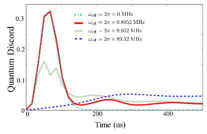
We plot the QD in Fig. 11. Interestingly, in contrast to the negativity, the QD, at , becomes larger as is decreased. This can be explained in the following way: if is sufficiently large, the state becomes a highly entangled state well approximated by the form
| (35) |
which decays, due the measurement of the nonlinear cavity, to the mixture
| (36) |
where and are high and low amplitude states of the nonlinear resonator. Since and are orthogonal to each other, is a classically correlated state without any superposition, implying vanishing QD. On the other hand, when is small, the dynamics can be explained by an AC Stark shift and the state can be expressed as
| (37) | |||||
where is the probability that the nonlinear resonator is in the low (or high) amplitude state. The state is the ground state of . Here, and are not always orthogonal to each other, and as such the correlation in the mixture of the two could have a non-classical nature. Hence, the QD, in the long-time limit, tends to have a finite value when is small.
VI Measurement of initial states not in the energy eigenbasis
Conventionally, in evaluating the performance of a readout device, one considers how well the final state of the measurement device correlates with the different possible initial states of the system, as discussed in trajectory ; clerk1 . In our case, this conventional approach does not reveal sufficient information about how well one can project something like the ground state of a USC system onto a non-eigenstate.
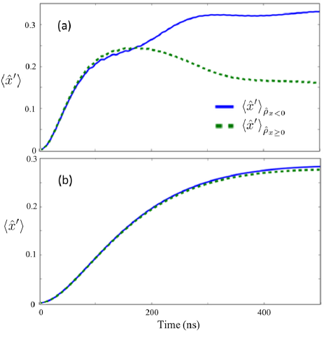
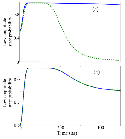
For example, in Fig. 12 we plot the probability for the resonator to be a low amplitude state depending on the initial states of the USC system. In particular, we choose these different states to be not eigenstates of the system Hamiltonian but eigenstates of the operator (in the two-level system approximation) which couples to the measurement device. These eigenstates correspond to and in the full basis, as described in the previous section. From these graphs, we can see that in the regime [Fig. 12(b)], there is no correlation between the state of the nonlinear resonator and the initial state of system. On the other hand, for much stronger couplings between system and measurement device, [Fig. 12(a)], there is a strong correlation between the nonlinear resonator and the initial state of the system.
These figures suggest that, in this conventional picture, the coupling strength should be comparable with the effective energy of the system to realize a measurement of an initial state which is not in an eigenstate of the Hamiltonian. This is because, when the initial state is not such an eigenstate, the qubit evolves under the system Hamiltonian with a time scale corresponding to the inverse of the eigenenergy (in this case, ). If the interaction between the system and measurement apparatus is much weaker than the eigenenergy of the system Hamiltonian, the system initial state evolves before the measurement apparatus obtains information about that initial state, and so the non-linear resonator has no time to build a correlation with the initial state of the system.
On the other hand, if the system is prepared in the ground state of the system Hamiltonian, the system does not, initially, evolve under the system Hamiltonian. This gives time for the the measurement apparatus to build up significant amount of photons, and become correlated with the system, due to the AC Stark shift, even in the regime of , as shown in the earlier sections of this work.
VII Conclusions
In conclusion, we investigated quantum measurements in the ultra-strong-coupling regime of a light-matter system. In particular, we showed how the ground state of an ultra-strongly-coupled system can be measured by a nonlinear resonator. Interestingly, we found that, even if the coupling strength with the measurement device is two orders of magnitude smaller than the typical energy scale of the ultra-strongly-coupled system, we can still induce a strong classical correlation with the measurement device. Also, we confirmed that, by increasing the coupling strength with the measurement device, entanglement between the system and measurement device can be generated, and we can realize projective measurements on the ground state of the ultra-strongly-coupled system. In addition, we found that the quantum discord tends to have a finite value at large times in the regime when the dynamics can be described by AC Stark shift. Our results help illuminate the mechanism of how an ultra-strongly coupled system interacts with a measurement device.
Acknowledgements.
We acknowledge helpful discussions with R. Stassi and H. Toida. This work was supported by JSPS KAKENHI Grants 15K17732 and MEXT KAKENHI Grant Number 15H05870. FN acknowledges support from the MURI Center for Dynamic Magneto-Optics via the AFOSR Award No. FA9550-14-1-0040, the Japan Society for the Promotion of Science (KAKENHI), the IMPACT program of JST, JSPS-RFBR grant No 17-52-50023, CREST grant No. JPMJCR1676. NL and FN acknowledge support by the Sir John Templeton Foundation and the RIKEN-AIST Joint Research Fund.Appendix A: Non-energy-eigenbasis measurements
Here, we explain the reason why the non-energy eigenbasis measurement is difficult to realize. Naive calculations indicate that the non-energy eigenbasis measurements would require a violation of the rotating wave approximation, which needs a strong coupling between the system and apparatus. This seems to suggest that, unless the coupling between the system and measurement apparatus is as large as the resonant frequency of the system and measurement apparatus, it would be difficult to implement the non-energy basis measurements. However, our results show that this naive picture is actually wrong if we use the non-linear resonator as a measurement apparatus.
We can explain these points more quantitatively as follows. Suppose the Hamiltonian which expresses the coupling between a qubit and a linear resonator as follows.
| (38) |
In a rotating frame defined by a unitary operator , we obtain
| (39) |
In the limit of a large , we can use a rotating wave approximation and we obtain
| (40) |
in the rotating frame.
More generally, we have a hamiltonian
| (41) |
where and , (the superindex (S) denotes the system and the superindex (E) denotes the measurement apparatus). In a rotating frame defined by , we have
| (42) | ||||
where . If the system and measurement apparatus are well detuned, we obtain
| (43) |
where we used the rotating wave approximation. So the terms that commute with survive. This clearly shows that we can measure only an observable that commutes with if the rotating wave approximation is valid. This also means that we need a violation of the rotating wave approximation for the non-energy eigenbasis measurements.
Appendix B: Derivation of the interaction Hamiltonian between the nonlinear resonator and the qubit
In this work we rely on an interaction between a superconducting flux qubit coupled with a frequency tunable resonator. This is not a dispersive approximation to a dipolar coupling. In more detail, the flux qubit is described as
| (44) |
where denotes an energy bias and denotes a tunneling energy. The Pauli matrix denotes a population of a persistent current basis such as where denotes a left-sided (right-handed) persistent current.
The frequency tunable resonator is described as
| (45) |
where denotes a frequency of the resonator. We assume that the resonator contains a SQUID structure, and we can tune the frequency of the resonator by changing an applied flux penetrating the SQUID structure. (For example, see reso1 ).
We can derive the interaction between the flux qubit and resonator as follows. The persistent current states of the flux qubit induces magnetic fields due to the Biot-Savart law, and this changes the penetrating magnetic flux of the SQUID in the resonator. So the frequency of the resonator depends on the state of the flux qubit. Suppose that () denotes the magnetic flux from the () state, and the resonator frequency will be approximately shifted by (). This provides us with the following Hamiltonian.
| (46) |
where . A similar Hamiltonian has been derived in reso2 to represented a coupling between an NV center and flux qubit.
Note that we assume a large detuning between the flux qubit and resonator. In this case dipolar coupling is negligible.
Appendix C: Derivation of the coarse graining measurement
In the case that there is noise in the measurement apparatus, when we have a position measurement, even if the result of the measurement apparatus is , the real value is not necessarily . To model such situations, we define a measurement operator as follows
| (47) |
where implies the strength of the noise. satisfies the normalization condition
| (48) |
Here, we consider a composite system which comprises of a system which we hope to readout (ultra-strongly coupled system) and its probe (nonlinear resonator). Also, the measurement result is divided to and . When we have a measurement on a composite system , the post measurement state when the result is becomes
| (49) | |||
where
| (50) |
By tracing out the probe system, we have the post measurement state of the system we hope to readout as
| (51) |
Substituting , can be rewritten as
| (52) |
where is a complementary error function, and is defined as
| (53) |
In the limit of , we have
| (54) |
which is noiseless measurement. Also, in the limit of , we obtain
| (55) |
which shows we cannot have any information from the system.
Appendix D: Validity of the two level approximation
VII.1 Adiabatic approximation to the Rabi Hamiltonian
We now explain the adiabatic approximation to the Rabi Hamiltonian, that has also been used in previous works ultra1 ; ultra2 ; ultra3 ; ultra4 . We will show that, within the framework of the adiabatic approximation, the ultra-strongly coupled system can be treated as a two-level system. The conventional Rabi Hamiltonian can be written as
| (56) |
The adiabatic approximation can be done when and the Rabi Hamiltonian can be diagonalized using the bases
| (57) | ||||
| (58) | ||||
| (59) |
where and are eigenstates of , is the level of the eigenstates of , and is a displacement operator. The states and are degenerate in energy and their energy is . Then, considering that the term couples these terms, and only the transitions between the states of the same are taken into account in the adiabatic approximation, the Rabi hamiltonian can be rewritten as
| (60) | |||
where
| (61) |
whose eigenvalues are
| (62) |
Also, it can be easily shown
| (63) | ||||
| (64) |
So, as long as we apply the adiabatic approximation, the transition due to the term is between and . Since the interaction between the ultra-strongly coupled system and the non-linear resonator can be expressed as , it is possible for us to consider that the ultra-strongly coupled system is driven only by the operator. Also, if the initial state is and the perturbation term is proportional only to (which applies to our system, which is composed of a ultra-strongly coupled system and a nonlinear resonator, where the interaction term can be expressed as ), the dynamics is limited to . Therefore, as long as the adiabatic approximation is valid, we can consider our system of the ultra-strongly coupled system as a two-level system.
VII.2 Estimation of the deviation from the two-level approximation.
By calculating the deviation from the two-level approximation, we show a quantitative analysis how accurate the two-level system approximation is in our parameter regime. We consider a fidelity between the true ground state (the first excited state ) and (.) It is possible to estimate the accuracy of our two-level approximation from this fidelity, and we derive a condition of the fidelity to be close to the unity. Now, we define
| (65) | |||
and
| (66) |
Here, is the one defined in Eq. 56. In this way, we regard as the non-perturbative Hamiltonian and the perturbative Hamiltonian. By performing a perturbative calculation up to the lowest order, we obtain
| (67) |
where is a normalization factor. Then by using perturbation theory, we have
| (68) | ||||
| (69) | ||||
| (70) |
In the perturbative calculation, the eigenstate after adding the perturbative term is not normalized to unity, and so we consider a normalization factor for such as
| (71) |
It can be easily shown that
| (72) |
and
| (73) |
Then, we have
| (74) | ||||
Then, by assuming , we have
| (75) | ||||
| (76) |
And, we have
| (77) | ||||
where
| (78) |
Also, we set
Similarly, with regard to the first excited state, we can obtain
| (79) | ||||
(Note that in Eq. 77 and Eq. VII.2 are the same.) The fidelity and are calculated as
| (80) | ||||
| (81) |
Then, we define
| (82) |
For , we have , and so we can consider as an infidelity.
We plot for three regimes . Here, we fix . From Fig. 13, we can see that in these regimes the infidelity is sufficiently small.
Also, we plot the numerically calculated
| (83) |
in Fig. 14 in the same regime where , , are the second, third and fourth excited states, respectively. This shows the leakage from to unwanted states.
Appendix E: Losses in the ultra-strongly coupled system
So far we did not include a full analysis of the USC losses because we assumed that the time scale of such losses would be much longer than the readout time. For completeness, here we present an short analysis of the influence of such losses. Because including bath-induced transitions between all eigenstates in the full space is complex, here we restrict ourselves to the two-level approximation. We justify this approximation, in our relevant parameter regime, in the previous sections.
The interaction Hamiltonian between our ultra-strongly coupled system and environment is described as
| (84) |
where denotes the position operator and () denotes the environmental operator coupled with the resonator (qubit). Also, we incorporate the effect of a dephasing bath classically modeled as
| (85) |
where is a time-dependent random variable and the ensemble average of is zero. In this case, it is well know that the Born-Markov-Secular Lindblad master equation can be written in the form ultra3
| (86) | ||||
| (87) |
where is the system Hamiltonian and
| (89) |
and
| (90) |
Here, and are the eigenstates of the system Hamiltonian and and is the rate corresponding to the noise spectra of the qubit and resonator, respectively. Also,
| (91) |
and
| (92) |
where denotes the spectral density of the qubit dephasing at frequency . Here, we ignore the term as this term is negligible when we operate at the “sweet spot” of the qubit. Owing to the two-level approximation, we consider only the lowest first two levels and , and defining , and , we obtain
| (93) | ||||
| (94) |
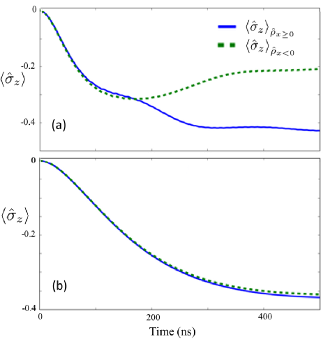
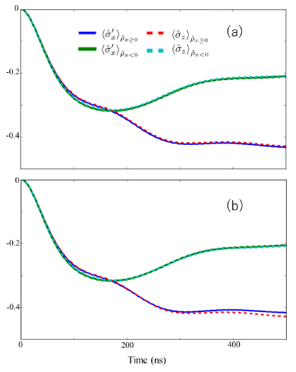
where . In Fig. 15(a), we plot the expectation value of and without the noise in the ultra-strongly coupled system. The two-level approximation shows an excellent agreement with the full Hamiltonian model. Also, in Fig. 15(b), we plot and including the noise in the ultra-strongly-coupled system with parameters fqyou that are realized in recent experiments fqdecay . From these results, we can conclude that the noise in the ultra-strongly coupled system is almost negligible and does not have significance on the time scales in which we are interested.
References
- (1) J. von Neumann, “Mathematical Foundations of Quantum Mechanics” (Princeton Univ. Press, Princeton, 1955);
- (2) V. B. Braginsky, Y. I. Vorontsov, K. S. Thorne, Quantum Nondemolition Measurement, Science, , 4456, 547, (1980).
- (3) T. Takano, M. Furuya, R. Namiki, and Y. Takahashi, Spin squeezing of a cold atomic ensemble with the nuclear spin of one-half, Phys. Rev. Lett. , 033601 (2009).
- (4) I. Siddiqi, R. Vijay, M. Metcalfe, E. Boaknin, L. Frunzio, R. J. Schoelkopf, and M. H. Devoret, Dispersive measurements of superconducting qubit coherence with a fast latching readout, Phys. Rev. B , 054510 (2006).
- (5) A. Lupascu, S. Saito, T. Picot, P. C. de Groot, C. J. P. M. Harmans and J. E. Mooij, Quantum non-demolition measurement of a superconducting two-level system, Nature Physics , 119 - 125 (2007).
- (6) N. Boulant, G. Ithier, P. Meeson, F. Nguyen, D. Vion, D. Esteve, I. Siddiqi, R. Vijay, C. Rigetti, F. Pierre, and M. Devoret, Quantum nondemolition readout using a Josephson bifurcation amplifier, Phys. Rev. B , 014525 (2007).
- (7) M. J. Biercuk, H. Uys, A. P. VanDevender, N. Shiga, W. M. Itano, and J. J. Bollinger, Optimized dynamical decoupling in a model quantum memory, Nature (London) , 996 (2009).
- (8) J. Bylander, S. Gustavsson, F. Yan, F. Yoshihara, K. Harrabi, G. Fitch, D. G. Cory, Y. Nakamura, J.-S. Tsai, and W. D. Oliver, Noise spectroscopy through dynamical decoupling with a superconducting flux qubit, Nat. Phys. , 565 (2011).
- (9) D. Ristè, C. C. Bultink, M. J. Tiggelman, R. N. Schouten, K. W. Lehnert, and L. DiCarlo, Millisecond charge-parity fluctuations and induced decoherence in a superconducting transmon qubit, Nat. Commun. , 1913 (2013).
- (10) C. C. Gerry and P.L. Knight, “Introductory Quantum Optics” (Cambridge University Press, Cambridge, 2005);
- (11) S. Ashhab, J. Q. You, and F. Nori, Weak and strong measurement of a qubit using a switching-based detector, Phys. Rev. A , 032317 (2009).
- (12) S. Ashhab, J. Q. You, and F. Nori, The information about the state of a qubit gained by a weakly coupled detector, New J. Phys. , 083017 (2009).
- (13) S. Ashhab, J. Q. You, F. Nori, The information about the state of a charge qubit gained by a weakly coupled quantum point contact, Phys. Scr. T, 014005 (2009).
- (14) M. Wallquist, K. Hammerer, P. Rabl, M. Lukin, and Zoller, P. Hybrid quantum devices and quantum engineering. Phys. Scr. , 014001 (2009).
- (15) T. Duty, Towards superconductor-spin ensemble hybrid quantum systems. Physics , 80 (2010).
- (16) Z. Xiang, S. Ashhab, J. Q. You, and F. Nori, Hybrid quantum circuits: superconducting circuits interacting with other quantum systems, Rev. Mod. Phys. , 623–653 (2013).
- (17) I. Buluta, S. Ashhab, and F. Nori, Natural and artificial atoms for quantum computation Reports on Progress in Physics , 104401 (2011)
- (18) I. Georgescu, F. Nori, Quantum technologies: an old new story, Physics World , 16-17 (2012).
- (19) X. Zhu, Y. Matsuzaki, R. Amsűss, K. Kakuyanagi, T. Shimo-Oka, N. Mizuochi, K. Nemoto, K. Semba, W. J. Munro and S. Saito, Observation of dark states in a superconductor diamond quantum hybrid system, Nature Communications , 3424 (2014).
- (20) K. Kakuyanagi, Y. Matsuzaki, C. Déprez, H. Toida, K. Semba, H. Yamaguchi, W. J. Munro, and S. Saito, Observation of Collective Coupling between an Engineered Ensemble of Macroscopic Artificial Atoms and a Superconducting Resonator, Phys. Rev. Lett. , 210503 (2016).
- (21) X. Wang, A. Miranowicz, H. R. Li, and F. Nori, Multiple-output microwave single-photon source using superconducting circuits with longitudinal and transverse couplings, Phys. Rev. A, , 053858 (2016).
- (22) N. Lambert, M. Cirio, M. Delbecq, G. Allison, M. Marx, S. Tarucha, F. Nori, Amplified and tunable transverse and longitudinal spin-photon coupling in hybrid circuit-QED, Phys. Rev. B, , 125429 (2018).
- (23) S. Ashhab and F. Nori. Qubit-oscillator systems in the ultrastrong-coupling regime and their potential for preparing nonclassical states, Phys. Rev. A , 042311(2011).
- (24) Y. Zhang, G. Chen, L. Yu, Q. Liang, J.-Q. Liang, and S. Jia, Analytical ground state for the Jaynes-Cummings model with ultrastrong coupling, Phys. Rev. A , 065802 (2011).
- (25) F. Beaudoin, J. M. Gambetta, and A. Blais, Dissipation and ultrastrong coupling in circuit QED, Phys. Rev. A , 043832 (2011).
- (26) S. Agarwal, S. M. Hashemi Rafsanjani and J. H. Eberly, Dissipation of the Rabi model beyond the rotating wave approximation: Quasi-degenerate qubit and ultra-strong coupling, J. Phys. B. , 224017(2013).
- (27) P. Nataf and C. Ciuti, Protected quantum computation with multiple resonators in ultrastrong coupling circuit QED, Phys. Rev. Lett. , 190402 (2011)
- (28) R. Stassi and F. Nori, Quantum Memory in the Ultrastrong-Coupling Regime via Parity Symmetry Breaking, arXiv:1703.08951 (2017).
- (29) K. Rzążewski and K. Wodkiewicz, Phase Transitions, Two-Level Atoms, and the Term, Phys. Rev. Lett. , 432 (1975).
- (30) S. Felicetti, T. Douce, G. Romero, P. Miliman and E. Solano, Parity-dependent State Engineering and Tomography in the ultrastrong coupling regime, Sci. Rep. , , 11818, (2015).
- (31) X. Cao, J. Q. You, H. Zheng, A.G. Kofman, F. Nori, Dynamics and quantum Zeno effect for a qubit in either a low- or high-frequency bath beyond the rotating-wave approximation, Phys. Rev. A , 022119 (2010).
- (32) X. Cao, J .Q. You, H. Zheng, F. Nori, A qubit strongly coupled to a resonant cavity: asymmetry of the spontaneous emission spectrum beyond the rotating wave approximation, New Journal of Physics , 073002 (2011).
- (33) X. Cao, Q. Ai, C. P. Sun, F. Nori, The transition from quantum Zeno to anti-Zeno effects for a qubit in a cavity by varying the cavity frequency, Phys. Lett. A , pp. 349-357 (2012).
- (34) L. Garziano, R. Stassi, V. Macrì, A.F. Kockum, S. Savasta, F. Nori, Multiphoton quantum Rabi oscillations in ultrastrong cavity QED, Phys. Rev. A , 063830 (2015).
- (35) L. Garziano, V. Macri, R. Stassi, O. D. Stefano, F. Nori, S. Savasta, One Photon Can Simultaneously Excite Two or More Atoms, Phys. Rev. Lett. , 043601 (2016).
- (36) O. D. Stefano, R. Stassi, L. Garziano, A.F. Kockum, S. Savasta, F. Nori, Feynman-diagrams approach to the quantum Rabi model for ultrastrong cavity QED: stimulated emission and reabsorption of virtual particles dressing a physical excitation, New Journal of Physics , 053010 (2017).
- (37) A. F. Kockum, A. Miranowicz, V. Macrì, S. Savasta, F. Nori, Deterministic quantum nonlinear optics with single atoms and virtual photons, Phys. Rev. A , 063849 (2017).
- (38) A. F. Kockum, V. Macrì, L. Garziano, S. Savasta, F. Nori, Frequency conversion in ultrastrong cavity QED, Scientific Reports , 5313 (2017).
- (39) R. Stassi, V. Macrì, A. F. Kockum, O.D. Stefano, A. Miranowicz, S. Savasta, F. Nori, Quantum Nonlinear Optics without Photons, Phys. Rev. A , 023818 (2017).
- (40) X. Wang, A. Miranowicz, H. R. Li, F. Nori, Observing pure effects of counter-rotating terms without ultrastrong coupling: A single photon can simultaneously excite two qubits, Phys. Rev. A , 063820 (2017).
- (41) F. Yoshihara, T. Fuse, S. Ashhab, K. Kakuyanagi, S. Saito and K. Semba, Superconducting qubit-oscillator circuit beyond the ultrastrong-coupling regime, Nature Physics 13, 44–47 (2017).
- (42) P. Forn-Diaz, J. J. Garcia-Ripoll, B. Peropadre, J.-L. Orgiazzi, M. A. Yurtalan, R. Belyansky, C. M. Wilson and A. Lupascu, Ultrastrong coupling of a single artificial atom to an electromagnetic continuum in the nonperturbative regime, Nature Physics , 39–43 (2017).
- (43) Z. Chen, Y. Wang, T. Li, L. Tian, Y. Qiu, K. Inomata, F. Yoshihara, S. Han, F. Nori, J. S. Tsai, and J. Q. You, Single-photon-driven high-order sideband transitions in an ultrastrongly coupled circuit-quantum-electrodynamics system, Phys. Rev. A , 012325 (2017).
- (44) S. De Liberato, D. Gerace, I. Carusotto, and C. Ciuti, Extracavity quantum vacuum radiation from a single qubit, Phys. Rev. A. 80, 053810, (2009).
- (45) C. K. Anderson and A. Blais, Ultrastrong coupling with a transmon qubit, New J. Phys. , 023022 (2017).
- (46) J. R. Johansson, G. Johansson, C. M. Wilson, and F. Nori, Dynamical Casimir effect in a superconducting coplanar waveguide, Phys. Rev. Lett. , 147003 (2009).
- (47) J. R. Johansson, G. Johansson, C.M. Wilson, and F. Nori, Dynamical Casimir effect in superconducting microwave circuits, Phys. Rev. A , 052509 (2010).
- (48) C. M. Wilson, G. Johansson, A. Pourkabirian, J.R. Johansson, T. Duty, F. Nori, and P. Delsing, Observation of the dynamical Casimir effect in a superconducting circuit, Nature , 376 (2011).
- (49) P. D. Nation, J.R. Johansson, M.P. Blencowe, F. Nori, Stimulating uncertainty: Amplifying the quantum vacuum with superconducting circuits, Rev. Mod. Phys. , 1-24 (2012).
- (50) J. R. Johansson, G. Johansson, C.M. Wilson, P. Delsing, F. Nori, Nonclassical microwave radiation from the dynamical Casimir effect, Phys. Rev. A , 043804 (2013).
- (51) R. Stassi, A. Ridolfo, O. Di Stefano, M.J. Hartmann and S. Savasta, Spontaneous conversion from virtual to real photons in the ultrastrong-coupling regime, Phys. Rev. Lett. 110, 243601, (2013).
- (52) M. Cirio, S. De Liberato, N. Lambert, and F. Nori, Ground State Electroluminescence, Phys. Rev. Lett. 116, 113601, (2016).
- (53) J. Lolli, A. Baksic, D. Nagy, V. E. Manucharyan, and C. Ciuti, Ancillary Qubit Spectroscopy of Vacua in Cavity and Circuit Quantum Electrodynamics, Phys. Rev. Lett. , 183601 (2015).
- (54) M. Cirio, K. Debnath, N. Lambert, F. Nori, Amplified Optomechanical Transduction of Virtual Radiation Pressure, Phys. Rev. Lett. , 053601 (2017).
- (55) H. Nakano, S. Saito, K. Semba and H. Takayanagi, Quantum Time Evolution in a Qubit Readout Process with a Josephson Bifurcation Amplifier, Phys. Rev. Lett. , 257003 (2009).
- (56) J. Gambetta, A. Blais, M. Boissonneault, A. A. Houck, D. I. Schuster and S. M. Girvin, Quantum trajectory approach to circuit QED: Quantum jumps and the Zeno effect, Phys. Rev. A, , 012112 (2008).
- (57) M. Boissonneault, A. C. Doherty, F. R. Ong, P. Bertet, D. Vion, D. Esteve and A. Blais, Back-action of a driven nonlinear resonator on a superconducting qubit, Phys. Rev. A , 022305 (2012).
- (58) U. Vool, S. Shankar, S. O. Mundhada, N. Ofek, A. Narla, K. Sliwa, E. Zalys-Geller, Y. Liu, L. Frunzio, R. J. Schoelkopf, S. M. Girvin, and M. H. Devoret, Continuous Quantum Nondemolition Measurement of the Transverse Component of a Qubit, Phys. Rev. Lett. , 133601 (2016).
- (59) K. Kakuyanagi, T. Baba, Y. Matsuzaki, H. Nakano, S. Saito and K. Semba, Observation of quantum Zeno effect in a superconducting flux qubit, New J. Phys. (2015).
- (60) K. Kakuyanagi, Y. Matsuzaki, T. Baba, H. Nakano, S. Saito, K. Semba, Characterization and Control of Measurement-Induced Dephasing on Superconducting Flux Qubit with a Josephson Bifurcation Amplifier. J. Phys. Soc. Jpn. , 104801 (2016).
- (61) I. Siddiqi, R. Vijay, F. Pierre, C. M. Wilson, M. Metcalfe, C. Rigetti, L. Frunzio, and M. H. Devoret, RF-Driven Josephson Bifurcation Amplifier for Quantum Measurement, Phys. Rev. Lett. , 207002 (2004).
- (62) K. Kakuyanagi, S. Kagei, R. Koibuchi, S. Saito, A. Lupascu, K. Semba and H. Nakano, Experimental analysis of the measurement strength dependence of superconducting qubit readout using a Josephson bifurcation readout method, New J. Phys. (2013).
- (63) M. O. Scully and M. S. Zubairy, Quantum Optics (Cambridge University Press, Cambridge, 1997).
- (64) M. Rigo, G. Alber, F. Mota-Furtado and P. F. O’Mahony, Quantum-state diffusion model and the driven damped nonlinear oscillator, Phys. Rev. A , 1665 (1997).
- (65) C. Laflamme and A. A. Clerk, Quantum-limited amplification with a nonlinear cavity detector, Phys. Rev. A 83, 033803 (2011).
- (66) C. Laflamme and A. A. Clerk, Weak Qubit Measurement with a Nonlinear Cavity: Beyond Perturbation Theory, Phys. Rev. Lett. , 123602 (2012).
- (67) C. Gardiner and P. Zoller, Quantum Noise (Springer, 2004)
- (68) H. Jeong, Y. Lim, and M. S. Kim, Coarsening Measurement References and the Quantum-to-Classical Transition, Phys. Rev. Lett. , 010402 (2014).
- (69) M. Krishnan V, T. Biswas, and S. Ghosh, Coarse-graining of measurement and quantum-to-classical transition in the bipartite scenario, arXiv: 1707.09951 (2017).
- (70) A. Ridolfo, M. Leib, S. Savasta, and M. J. Hartmann, Photon Blockade in the Ultrastrong Coupling Regime, Phys. Rev. Lett. , 193602 (2012).
- (71) L. Garziano, A. Ridolfo, R. Stassi, O. Di Stefano, and S. Savasta, Switching on and off of ultrastrong light-matter interaction: Photon statistics of quantum vacuum radiation, Phys. Rev. A , 063829 (2013).
- (72) R. Stassi, S. Savasta, L. Garziano, B. Spagnolo and F. Nori, Output field-quadrature measurements and squeezing in ultrastrong cavity-QED, New J. Phys. , 123005 (2016).
- (73) J. R. Johansson, P.D. Nation, and F. Nori, QuTiP 2: A Python framework for the dynamics of open quantum systems, Comp. Phys. Comm. , 1234 (2013).
- (74) J. R. Johansson, P.D. Nation, and F. Nori, QuTiP: An open-source Python framework for the dynamics of open quantum systems, Comp. Phys. Comm. , 1760 (2012).
- (75) An introduction to entanglement measures, MB Plenio, S Virmani, arXiv preprint, quant-ph/0504163, (2005).
- (76) H. Ollivier and W. H. Zurek, Quantum Discord: A Measure of the Quantumness of Correlations, Phys. Rev. Lett. , 017901 (2001).
- (77) L. Henderson and V. Vedral: Classical, quantum and total correlations, J. Phys. A , 6899 (2001).
- (78) Y. Kubo, F. R. Ong, P. Bertet Strong Coupling of a Spin Ensemble to a Superconducting Resonator, Phys. Rev. Lett, , 140502 (2010).
- (79) D. Marcos, M. Wubs, J. M. Taylor Coupling Nitrogen-Vacancy Centers in Diamond to Superconducting Flux Qubits, Phys. Rev. Lett. 105, 210501 (2010).
- (80) J. Q. You, Xuedong Hu, S. Ashhab, and F. Nori, Low-decoherence flux qubit, Phys. Rev. B , 140515(R) (2007).
- (81) F. Yan, S. Gustavsson , The flux qubit revisited to enhance coherence and reproducibility, Nat. Commun. , 12964 (2016).