The effect of polydispersity in a turbulent channel flow laden with finite-size particles

Abstract

We study turbulent channel flows of monodisperse and polydisperse suspensions of finite-size spheres by means of Direct Numerical Simulations using an immersed boundary method to account for the dispersed phase. Suspensions with 3 different Gaussian distributions of particle radii are considered (i.e. 3 different standard deviations). The distributions are centered on the reference particle radius of the monodisperse suspension. In the most extreme case, the radius of the largest particles is 4 times that of the smaller particles. We consider two different solid volume fractions, $2\%$ and $10\%$. We find that for all polydisperse cases, both fluid and particles statistics are not substantially altered with respect to those of the monodisperse case. Mean streamwise fluid and particle velocity profiles are almost perfectly overlapping. Slightly larger differences are found for particle velocity fluctuations. These increase close to the wall and decrease towards the centerline as the standard deviation of the distribution is increased. Hence, the behavior of the suspension is mostly governed by excluded volume effects regardless of particle size distribution (at least for the radii here studied). Due to turbulent mixing, particles are uniformly distributed across the channel. However, smaller particles can penetrate more into the viscous and buffer layer and velocity fluctuations are therein altered. Non trivial results are presented for particle-pair statistics.

I Introduction

Particle laden flows are relevant in several industrial applications and many natural and environmental processes. Among these we recall the sediment transport in rivers, avalanches and pyroclastic flows, plankton in seas, planetesimals in accretion disks, as well as many oil industry and pharmaceutical processes. In most cases the carrier phase is a turbulent flow due to the high flow rates. However, due to the interaction between particles and vortical structures of different sizes the turbulence properties can be substantially altered and the flow may even be relaminarized. Additionally, particles may differ in density, shape, size and stiffness. The prediction of the suspension rheological behavior is hence a complex task.

Interesting and peculiar rheological properties can be observed already in the viscous and low-speed laminar regimes, and for suspensions of monodispersed rigid spheres. Depending for example on the shear rate and on particle concentration, suspensions can exhibit shear thinning or thickening, jamming (at high volume fractions), and the generation of high effective viscosities and normal stress differences stickel2005 ; morris2009 ; wagner2009 . More generally, due to the dispersed solid phase, the fluid response to the local deformation rate is altered and the resulting suspension effective viscosity $\mu_{e}$ differs from that of the pure fluid $\mu$guazz2011 ; einstein1906 ; einstein1911 ; batchelor1970 . In laminar flows, when the particle Reynolds number $Re_{a}$ becomes non negligible, the symmetry of the particle pair trajectories is broken and the microstructure becomes anisotropic. This leads to macroscopical behaviors such as shear-thickening and the occurrence of normal stress differencesMorrispof08 ; picano2013 ; Morris2014 . Recently, it was also shown that in simple shear flows, the effective viscosity $\mu_{e}$ depends non-monotonically on the system confinement (i.e. the gap size in a Couette flow). In particular, minima of $\mu_{e}$ are observed when the gap size is approximately an integer number of particle diameters, due to the formation of stable particle layers with low momentum exchange across layersfornariPRL . Finally, in the Bagnoldian or highly inertial regime the effective viscosity $\mu_{e}$ increases linearly with shear rate due to augmented particle collisions bagnold1954 .

When particles are dispersed in turbulent flows, the dynamics of the fluid phase can be substantially modified. Already in the transition from the laminar to the turbulent regime, the presence of the solid phase may either increase or reduce the critical Reynolds number above which the transition occurs. Different groupsmatas2003 ; yu2013 studied for example, the transition in a turbulent pipe flow laden with a dense suspension of particles. They found that transition depends upon the pipe to particle diameter ratios and the volume fraction. For smaller neutrally-buoyant particles they observed that the critical Reynolds number increases monotonically with the solid volume fraction $\phi$ due to the raise in effective viscosity. On the other hand, for larger particles it was found that transition shows a non-monotonic behavior which cannot be solely explained in terms of an increase of the effective viscosity $\mu_{e}$. Concerning transition in dilute suspensions of finite-size particles in plane channels, it was shown that the critical Reynolds number above which turbulence is sustained, is reducedlashg2015 ; loisel2013 . At fixed Reynolds number and solid volume fraction, also the initial arrangement of particles was observed to be important to trigger the transition.
For channel flows laden with solid spheres, three different regimes have been identified for a wide range of solid volume fractions $\phi$ and bulk Reynolds numbers $Re_{b}$lashgari2014 . These are laminar,turbulent and inertial shear-thickening regimes and in each case, the flow is dominated by different components of the total stress: viscous, turbulent or particle stresses.

In the fully turbulent regime, most of the previous studies have focused on dilute or very dilute suspensions of particles smaller than the hydrodynamic scales and heavier than the fluid. In the one-way coupling regime balach-rev2010 (i.e. when the solid phase has a negligible effect on the fluid phase), it has been shown that particles migrate from regions of high to low turbulence intensities reeks1983 . This phenomenon is known as turbophoresis and it is stronger when the turbulent near-wall characteristic time and the particle inertial time scale are similar soldati2009 . In these inhomogeneous flows, Sardina et al.sardina2011 ; sardina2012 also observed small-scale clustering that together with turbophoresis leads to the formation of streaky particle patterns sardina2011 . When the solid mass fraction is high and back-influences the fluid phase (i.e. in the two-way coupling regime), turbulence modulation has been observedkulick1994 ; zhao2010 . The turbulent near-wall fluctuations are reduced, their anisotropy increases and eventually the total drag is decreased.

In the four-way coupling regime (i.e. dense suspensions for which particle-particle interactions must be considered), it was shown that finite-size particles slightly larger than the dissipative length scale increase the turbulent intensities and the Reynolds stresses pan1996 . Particles are also found to preferentially accumulate in the near-wall low-speed streaks. This was also observed in open channel flows laden with heavy finite-size particles kida2013 .
On the contrary, for turbulent channel flows of denser suspensions of larger particles (with radius of about $10$ plus units), it was found that the large-scale streamwise vortices are attenuated and that the fluid streamwise velocity fluctuation is reducedshao2012 ; picano2015 . The overall drag increases as the volume fraction is increased from $\phi=0\%$ up to $20\%$. As $\phi$ is increased, turbulence is progressively reduced (i.e. lower velocity fluctuation intensities and Reynolds shear stresses). However, particle induced stresses show the opposite behavior with $\phi$, and at the higher volume fraction they are the main responsible for the overall increase in dragpicano2015 . Recently, Costa et al.costa2016 showed that if particles are larger than the smallest turbulent scales, the suspension deviates from the continuum limit. The effective viscosity alone is not sufficient to properly describe the suspension dynamics which is instead altered by the generation of a near-wall particle layer with significant slip velocity.

As noted by Prosperetti prosp2015 , however, results obtained for solid to fluid density ratios $R=\rho_{p}/\rho_{f}=1$ and for spherical particles, cannot be easily extrapolated to other cases (e.g. when $R>1$). This motivated researchers to investigate turbulent channel flows with different types of particles. For example, in an idealized scenario where gravity is neglected, we studied the effects of varying independently the density ratio $R$ at constant $\phi$, or both $R$ and $\phi$ at constant mass fraction, on both the rheology and the turbulencefornariPOF . We found that the influence of the density ratio $R$ on the statistics of both phases is less important than that of an increasing volume fraction $\phi$. However, for moderately high values of the density ratio ($R\sim 10$) we observed an inertial shear-induced migration of particles towards the core of the channel. Ardekani et al.ardekani2016 studied instead a turbulent channel flow laden with finite-size neutrally buoyant oblates. They showed that due to the peculiar particle shape and orientation close to the channel walls, there is clear drag reduction with respect to the unladen case.

In the present study we consider again finite-size neutrally buoyant spheres and explore the effects of polydispersity. Typically, it is very difficult in experiments to have suspension of precisely monodispersed spheres (i.e. with exactly the same diameter). On the other hand, direct numerical simulations (DNS) of particle laden flows are often limited to monodisperse suspensions. Hence, we decide to study turbulent channel flows laden with spheres of different diameters. Trying to mimic experiments, we consider suspensions with Gaussian distributions of diameters. We study 3 different distributions with $\sigma_{a}/(2a)=0.02,0.06$ and $0.1$, being $\sigma_{a}$ the standard deviation. For each case we have a total of 7 different species and the solid volume fraction $\phi$ is kept constant at $10\%$ (for each case the total number of particles is different). We then consider a more dilute case with $\phi=2\%$ and $\sigma_{a}/(2a)=0.1$. The reference spheres have radius of size $a=h/18$ where $h$ is the half-channel height. The statistics for all $\sigma_{a}/(2a)$ are compared to those obtained for monodisperse suspensions with same $\phi$. For all $\phi$, we find that even for the larger $\sigma_{a}/(2a)=0.1$ the results do not differ substantially from those of the monodisperse case. Slightly larger variations are found for particle mean and fluctuating velocity profiles. Therefore, rheological properties and turbulence modulation depend strongly on the overall solid volume fraction $\phi$ and less on the particle size distribution. We then look at probability density functions of particle velocities and mean-squared dispersions. For each species the curves are similar and almost overlapped. However, we identify a trend depending on the particle diameter. Finally, we study particle-pair statistics. We find that collision kernels between particles of different sizes (but equal concentration), resemble more closely those obtained for equal particles of the smaller size.

II Methodology

II.1 Numerical method

In the present study we perform direct numerical simulations and use an immersed boundary method to account for the presence of the dispersed solid phasebreugem2012 ; kempe2012 . The Eulerian fluid phase is evolved according to the incompressible Navier-Stokes equations,

$${\bf\nabla\cdot}{\bf u}_{f}=0$$ (1)

$$\frac{\partial{\bf u}_{f}}{\partial t}+{\bf u}_{f}\cdot{\bf\nabla}{\bf u}_{f}=-\frac{1}{\rho_{f}}{\bf\nabla}p+\nu{\bf\nabla}^{2}{\bf u}_{f}+{\bf f}$$ (2)

where ${\bf u}_{f}$, $\rho_{f}$, $p$ and $\nu=\mu/\rho_{f}$ are the fluid velocity, density, pressure and kinematic viscosity respectively ($\mu$ is the dynamic viscosity). The immersed boundary force ${\bf f}$, models the boundary conditions at the moving particle surface. The particles centroid linear and angular velocities, ${\bf u}_{p}$ and ${\bf\boldsymbol{\omega}}_{p}$ are instead governed by the Newton-Euler Lagrangian equations,

$$\rho_{p}V_{p}\frac{d{\bf u}_{p}}{dt} =\rho_{f}\oint_{\partial\mathcal{V}_{p}}{\bf\boldsymbol{\tau}}\cdot{\bf n}\,dS$$ (3)

$$I_{p}\frac{d{\bf\boldsymbol{\omega}}_{p}}{dt} =\rho_{f}\oint_{\partial\mathcal{V}_{p}}{\bf r}\times{\bf\boldsymbol{\tau}}\cdot{\bf n}\,dS$$ (4)

where $V_{p}=4\pi a^{3}/3$ and $I_{p}=2\rho_{p}V_{p}a^{2}/5$ are the particle volume and moment of inertia; ${\bf\boldsymbol{\tau}}=-p{\bf I}+2\mu{\bf E}$ is the fluid stress, with ${\bf E}=\left({\bf\nabla}{\bf u}_{f}+{\bf\nabla}{\bf u}_{f}^{T}\right)/2$ the deformation tensor; ${\bf r}$ is the distance vector from the center of the sphere while $\bf{n}$ is the unity vector normal to the particle surface $\partial\mathcal{V}_{p}$. Dirichlet boundary conditions for the fluid phase are enforced on the particle surfaces as ${\bf u}_{f}|_{\partial\mathcal{V}_{p}}={\bf u}_{p}+{\bf\boldsymbol{\omega}}_{p}\times{\bf r}$.
The fluid phase is evolved in the whole computational domain using a second order finite difference scheme on a staggered mesh. The time integration of both Navier-Stokes and Newton-Euler equations is performed by a third order Runge-Kutta scheme. A pressure-correction method is applied at each sub-step. Each particle surface is described by $N_{L}$ uniformly distributed Lagrangian points. The force exchanged by fluid and the particles is imposed on each $l-th$ Lagrangian point and is related to the Eulerian force field ${\bf f}$ by the expression ${\bf f}({\bf x})=\sum_{l=1}^{N_{L}}{\bf F}_{l}\delta_{d}({\bf x}-{\bf X}_{l})\Delta V_{l}$. In the latter $\Delta V_{l}$ represents the volume of the cell containing the $l-th$ Lagrangian point while $\delta_{d}$ is the Dirac delta. This force field is calculated through an iterative algorithm that ensures a second order global accuracy in space.
Particle-particle interactions are also considered. When the gap distance between two particles is smaller than twice the mesh size, lubrication models based on Brenner’s and Jeffrey’s asymptotic solutions (brenner1961, ; jeffrey1982, ) are used to correctly reproduce the interaction between the particles of different sizes. A soft-sphere collision model is used to account for collisions between particles and between particles and walls. An almost elastic rebound is ensured with a restitution coefficient set at $0.97$. These lubrication and collision forces are added to the Newton-Euler equations. For more details and validations of the numerical code, the reader is referred to previous publications breugem2012 ; lambert2013 ; fornari2015 .

II.2 Flow configuration

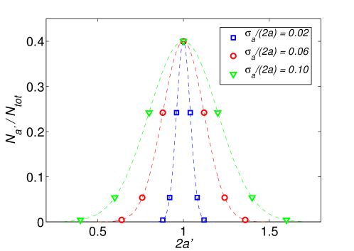
Figure 1: Fraction of particles with radius $a^{\prime}$, $N_{a^{\prime}}/N_{tot}$, for each Gaussian distribution.

We consider a turbulent channel flow between two infinite flat walls located at $y=0$ and $y=2h$, where $y$ is the wall-normal direction while $x$ and $z$ are the streamwise and spanwise directions. The domain has size $L_{x}=6h$, $L_{y}=2h$ and $L_{z}=3h$ with periodic boundary conditions imposed in the streamwise and spanwise directions. A mean pressure gradient is imposed in the streamwise direction to ensure a fixed value of the bulk velocity $U_{0}$. The imposed bulk Reynolds number is equal to $Re_{b}=U_{0}2h/\nu=5600$ and corresponds to a Reynolds number based on the friction velocity $Re_{\tau}=U_{*}h/\nu=180$ for the unladen case. The friction velocity is defined as $U_{*}=\sqrt{\tau_{w}/\rho_{f}}$, where $\tau_{w}$ is the stress at the wall. A staggered mesh of $1296\times 432\times 649$ grid points is used to discretize the domain. All results will be reported either in non-dimensional outer units (scaled by $U_{0}$ and $h$) or in inner units (with the superscript ’+’, using $U_{*}$ and $\delta_{*}=\nu/U_{*}$).

The solid phase consists of non-Brownian, neutrally buoyant rigid spheres of different sizes. In particular we consider Gaussian distributions of particle radii with standard deviations of $\sigma_{a}/(2a)=0.02,0.06$ and $0.1$. In figure 1 we show for each $\sigma_{a}/(2a)$, the fraction of particles with radius $a^{\prime}$, $N_{a^{\prime}}/N_{tot}$ (with $N_{tot}$ the total number of spheres). For all cases, the reference spheres have a radius to channel half-width ratio fixed to $a/h=1/18$. The reference particles are discretized with $N_{l}=1721$ Lagrangian control points while their radii are $12$ Eulerian grid points long. In figure 2 we display the instantaneous streamwise velocity on three orthogonal planes together with a fraction of the particles dispersed in the domain for $\sigma_{a}/(2a)=0.1$. In this extreme case, the size of the smallest and largest particles is $a^{\prime}/a=0.4$ and $1.6$. These particles are hence substantially smaller/larger than our reference spheres.

The simulations start from the laminar Poiseuille flow for the fluid phase since we observe that the transition naturally occurs at the present moderately high Reynolds number due to the noise added by the particles. Particles are initially positioned randomly with velocity equal to the local fluid velocity. Statistics are collected after the initial transient phase. At first, we will compare results obtained for denser suspensions with solid volume fraction $\phi=10\%$ and different $\sigma_{a}/(2a)$, with those of the monodisperse case ($\sigma_{a}/(2a)=0$). We will then discuss the statistics obtained for $\phi=2\%$ and $\sigma_{a}/(2a)=0$ and $0.1$. The full set of simulations is summarized in table 1.

$\phi($%$)$	$\sigma_{a}/(2a)$	$N_{p}$
$10$	$0$	$5012$
$10$	$0.02$	$4985$
$10$	$0.06$	$4802$
$10$	$0.10$	$4474$
$2$	$0$	$1002$
$2$	$0.10$	$896$

Table 1: Summary of the simulations performed ($N_{p}$ is the total number of particles).

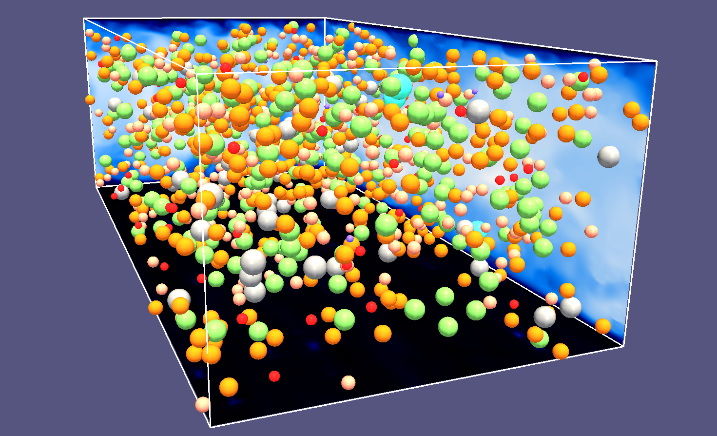
Figure 2: Instantaneous snapshot of the instantaneous streamwise velocity on three orthogonal planes together with a fraction of particles for the case $\sigma_{a}/(2a)=0.1$.

III Results

III.1 Fluid and particle statistics

We show in figure 3$(a)$ the mean fluid streamwise velocity profiles in outer units, $U(y)$, for $\sigma_{a}/(2a)=0,0.02,0.06$ and $0.1$. We find that the profiles obtained for monodisperse and polydisperse suspensions overlap almost perfectly. No differences are observed even for the case with larger variance $\sigma_{a}/(2a)=0.1$. In figures 3$(b),(c),(d)$ we then show the profiles of streamwise, wall-normal and spanwise fluctuating fluid velocities, $u_{f,rms}^{\prime},v_{f,rms}^{\prime},w_{f,rms}^{\prime}$. These profiles exhibit small variations and no precise trend (as function of $\sigma_{a}/(2a)$) can be identified. The larger variations between the cases are found close to the wall, $y\in(0.1;0.2)$, where the maximum intensity of the velocity fluctuations is found, and at the centerline. In the latter location, we notice that fluctuations are always smaller for $\sigma_{a}/(2a)=0.1$. In this case, many particles are substantially larger than the reference ones with $a^{\prime}/a=1$. Around the centerline these move almost undisturbed therefore inducing slightly smaller fluid velocity fluctuations.

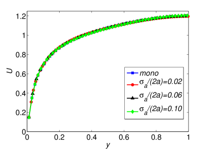
Figure 3: Mean fluid streamwise velocity profile (a) and fluid velocity fluctuations in the streamwise (b), wall-normal (c) and spanwise (d) directions for different standard deviations $\sigma_{a}/(2a)=0$, $0.02$, $0.06$, $0.1$.

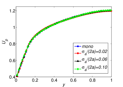
Figure 4: Mean particle streamwise velocity profile (a) and particle velocity fluctuations in outer and inner units, in the streamwise (b)-(c), wall-normal (d)-(e) and spanwise (f)-(g) directions, for different standard deviations $\sigma_{a}/(2a)=0$, $0.02$, $0.06$, $0.1$.

The mean particle streamwise velocity is reported in figure 4$(a)$. As for the fluid phase, no relevant difference is found in the profiles of $U_{p}(y)$ for the cases studied. Larger variations (also with respect to fluid velocity fluctuations) are found in the profiles of $u_{p,rms}^{\prime},v_{p,rms}^{\prime},w_{p,rms}^{\prime}$, depicted in outer units in figures 4$(b),(d),(f)$, and in inner units in figures 4$(c),(e),(g)$. From these we can identify two different trends. Very close to the wall (in the viscous sublayer), particle velocity fluctuations increase progressively as $\sigma_{a}/(2a)$ is increased, especially in the streamwise direction. This is probably due to the fact that as $\sigma_{a}/(2a)$ is increased, there are smaller particles that can penetrate more into the viscous and buffer layers. However, being smaller and having smaller inertia, they are more easily mixed in all directions due to turbulence structures, and hence experience larger velocity fluctuations. Secondly, we observe smaller velocity fluctuations around the centerline for $\sigma_{a}/(2a)=0.1$. As $\sigma_{a}/(2a)$ increases, larger particles are preferentially found at the centerline and move almost unperturbed in the streamwise direction, hence the reduction in $u_{p,rms}^{\prime},v_{p,rms}^{\prime},w_{p,rms}^{\prime}$. Between the viscous sublayer and the centerline, due to turbulence mixing it is difficult to identify an exact dependence on $\sigma_{a}/(2a)$.

Concerning the solid phase, we show in figure 5 the particle concentration profiles $\phi(y)$ across the channel. From figure 5$(a)$ we see that the concentration profiles are similar for all $\sigma_{a}/(2a)$. However, as previously mentioned we notice that as $\sigma_{a}/(2a)$ is increased, the peak located at $y\simeq 0.1$ is smoothed, while the concentration at the centerline is also increased. We then show in figures 5$(b),(d)$ the concentration profiles in logarithmic scale of the different species for the cases with $\sigma_{a}/(2a)=0.02$ and $0.1$; the counterparts in linear scales are shown in figures 5$(c),(e)$, where the curves of the species with larger and smaller diameters have been removed for clarity. If we compare the different curves to the reference case with $a^{\prime}/a=1$, we observe that the initial peak moves closer to and further from the walls for decreasing and increasing $a^{\prime}/a$. For larger $a^{\prime}/a$, the peak is also smoothed until it disappears for $a^{\prime}/a>1.2$ in the most extreme case with $\sigma_{a}/(2a)=0.1$. In the latter, for each species with $a^{\prime}/a>1$ the concentration grows with $y$ and reaches the maximum value at the centerline. On the other hand, the initial peak of the smallest particles is well inside the viscous sublayer.

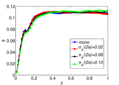
Figure 5: (a) Mean local volume fraction $\phi(y)$ in the wall-normal direction for different $\sigma_{a}/(2a)=0$, $0.02$, $0.06$, $0.1$. Mean local volume fraction for each particle species of the case with $\sigma_{a}/(2a)=0.02$: logarithmic (b) and linear (c). Mean local volume fraction for each particle species of the case with $\sigma_{a}/(2a)=0.1$: logarithmic (d) and linear (e).

We conclude this section by performing a stress analysis. Indeed, the understanding of the momentum exchange between fluid and solid phases in particle laden turbulent channel flows is conveniently addressed by examining the streamwise momentum or average stress budget. As in Picano et al.picano2015 we can write the total stress budget (per unit density) as the sum of three terms:

$$\tau=\tau_{V}+\tau_{T}+\tau_{P}$$ (5)

where $\tau=\left.\nu\frac{dU_{f,x}}{dy}\right|_{w}\left(1-\frac{y}{h}\right)$ is the total stress ($\left.\frac{d}{dy}\right|_{w}$ denotes a derivative taken at the wall), $\tau_{V}=\nu(1-\phi)\frac{dU_{f,x}}{dy}$ the viscous stress, $\tau_{T}=-\langle u_{c,x}^{\prime}u_{c,y}^{\prime}\rangle=-(1-\phi)\langle u_{f,x}^{\prime}u_{f,y}^{\prime}\rangle-\phi\langle u_{p,x}^{\prime}u_{p,y}^{\prime}\rangle$ the turbulent Reynolds shear stress of the combined phase, and $\tau_{P}=\phi\langle\sigma_{p,xy}/\rho_{f}\rangle$ the particle induced stress. Additionally, we define the particle Reynolds stress $\tau_{T_{p}}=-\phi\langle u_{p,x}^{\prime}u_{p,y}^{\prime}\rangle$. The total stress balance for the monodisperse case is shown in figure 6$(a)$ (the curves for the polydisperse suspensions are not depicted being the differences with the actual case negligible). We observe that the major contribution to $\tau$ comes from the turbulent Reynolds stress term $\tau_{T}$ and in particular from the contribution of the fluid phase (the particle Reynolds stress amounts to $\sim 10\%$ of $\tau_{T}$). The particle induced stress $\tau_{P}$ is important throughout the whole channel (though sub-leading with respect to $\tau_{T}$) and especially close to the wall. In figures 6$(b),(c),(d)$ we finally compare $\tau_{T}$, $\tau_{T_{p}}$ and $\tau_{P}$ for all $\sigma_{a}/(2a)$. Although the profiles for $\tau_{T}$ are almost perfectly overlapping, we observe that the maximum of $\tau_{T_{p}}$ and $\tau_{P}$ are slightly lower for $\sigma_{a}/(2a)=0.1$. Closer to the centerline $\tau_{P}$ is smaller for $\sigma/(2a)=0$ and $0.1$.
Next, we consider the friction Reynolds number $Re_{\tau}=U_{*}h/\nu$, for each case. For the monodisperse case we have $Re_{\tau}=196$ while for the polydisperse cases we obtain $Re_{\tau}=196,195$ and $194$ for $\sigma_{a}/(2a)=0.02,0.06$ and $0.1$. The friction Reynolds number is hence larger than that of the unladen case ($Re_{\tau}=180$) due to an enhanced turbulent actvity close to the wall, and to the presence of an additional dissipative mechanism introduced by the solid phase (i.e. $\tau_{P}$)picano2015 ; costa2016 . The fact that $Re_{\tau}$ is smaller for $\sigma_{a}/(2a)=0.1$ is related to the fact that the contribution to the total stress from both $\tau_{T_{p}}$ and $\tau_{P}$ is slightly reduced with respect to all other cases (see figures 6$(c),(d)$). The small discrepancy is however of the order of the statistical error.

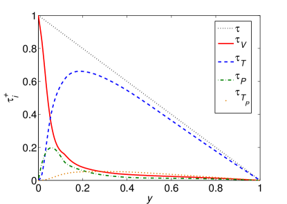
Figure 6: Shear-stress balance in the wall-normal direction (a). The overall stress $\tau$ is the sum of the viscous stress $\tau_{V}$, the turbulent stres $\tau_{T}$ (i.e. the Reynolds stress), and the particle-induced stress $\tau_{P}$; $\tau_{T_{P}}$ is the particle Reynolds stress. Comparison of the turbulent stress (b), particle turbulent stress (c), particle-induced stress (d) for different $\sigma_{a}/(2a)$.

The results presented clearly show that in turbulent channel flows laden with finite-size spheres, the key parameter in defining both rheological properties and turbulence modulation is the solid volume fraction $\phi$. Even in the most extreme case, $\sigma_{a}/(2a)=0.1$, for which the smallest and largest particles have radii of $0.4$ and $1.6$ times that of the reference particles, both fluid and particle statistics are similar to those of the monodisperse case. To gain further insight, we also look at the Stokes number of the different particles. The Stokes number $St_{a}$ is the ratio between the typical particle time scale and a characteristic flow time scale. We consider the convective time as flow characteristic time $T_{f}=h/U_{0}=2h^{2}/(Re_{b}\nu)$ and introduce the particle relaxation time defined as $T_{p}=4Ra^{2}/(18\nu)$. The effect of finite inertia (i.e. of a non negligible Reynolds number) is taken into account using the correction to the particle drag coefficient $C_{D}$ proposed by Schiller & Naumannschil1935 :

$$C_{D}=\frac{24}{Re_{a}}\left(1+0.15Re_{a}^{0.687}\right)$$ (6)

Assuming particle acceleration to be balanced only by the nonlinear Stokes drag, and the Reynolds number to be roughly constant, it can be found that $V(t)\sim exp\left(-t/T_{p}^{\prime}\right)$, where $T_{p}^{\prime}=T_{p}/\left(1+0.15Re_{a}^{0.687}\right)$. For sake of simplicity and in first approximation we define a shear-rate based particle Reynolds number $Re_{a}=Re_{b}(a/h)^{2}$. The final expression for the modified Stokes number is

$$St_{a}^{\prime}=\frac{T_{p}}{T_{f}}\frac{1}{\left(1+0.15Re_{a}^{0.687}\right)}=\left(\frac{2a}{h}\right)^{2}\frac{1}{36}Re_{b}R\frac{1}{\left(1+0.15Re_{a}^{0.687}\right)}$$ (7)

For the reference particles we obtain $Re_{a}=17.3$ and $St_{a}^{\prime}=0.93$. For the smallest particles ($a^{\prime}/a=0.4$) we find $Re_{a}=2.8$ and $St_{a}^{\prime}=0.24$, while for the largest ($a^{\prime}/a=1.6$) $Re_{a}=44.2$ and $St_{a}^{\prime}=1.63$. Hence, when the radius of the largest particles is $4$ times that of the smallest particles, there is an order of magnitude difference in the Stokes number. It is also interesting to note that albeit the use of a nonlinear drag correction, if we average the Stokes numbers of largest and smallest particles we get that of the reference case ($St_{a}^{\prime}=0.93$). Hence, $30\%$ of the particles respond more slowly to fluid-induced velocity perturbations than the reference particles, while other $30\%$ respond more quickly. On average, however, the suspension responds with a time scale comparable to that of the monodisperse case, therefore behaving similarly from a statistical perspective. We expect this to be the case for all volume fractions $\phi$ in this semi-dilute regime. This finding can be useful for modeling the behavior of rigid-particle suspensions.

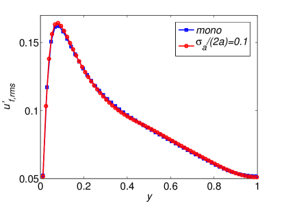
Figure 7: Fluid and particle velocity fluctuations in outer units, in the streamwise (a)-(b), wall-normal (c)-(d) and spanwise (e)-(f) directions, for $\sigma_{a}/(2a)=0$ and $0.1$.

To check this, we performed 2 additional simulations with $\phi=2\%$ and $\sigma_{a}/(2a)=0$ and $0.1$. The fluid and particle velocity fluctuations in the streamwise, wall-normal and spanwise directions are shown in figures 7$(a),(c),(e)$ and in figures 7$(b),(d),(f)$. The mean fluid and particle streamwise velocities are not reported since the curves are again almost perfectly overlapping. Regarding the fluid velocity fluctuation profiles, we see that the results of the mono and polydisperse cases are almost identical. As for $\phi=10\%$, particle velocity fluctuation profiles exhibit larger variations with respect to the monodisperse results. In particular, we notice that the profiles vary in a similar way for both $\phi$: smaller fluctuations throughout the channel, except in the viscous sublayer where the maxima of streamwise and wall-normal fluctuations are found ($y\in(0.1;0.2)$). However, the largest relative difference between the velocity fluctuation profiles of the mono and polydisperse cases is only about $7\%$.
Finally, we also computed the friction Reynolds number and found a similar behavior as for $\phi=10\%$. Indeed, for both $\phi$ and $\sigma_{a}/(2a)=0.1$, the friction Reynolds number $Re_{\tau}$ decreases by about $1\%$ with respect to the case with $\sigma_{a}/(2a)=0$. For $\phi=2\%$, $Re_{\tau}$ decreases from $186$ to $183$.

III.2 Single-point particle statistics

We wish to give further insight on the behavior of the solid phase dynamics by examining the probability density functions, $pdf$s, of particle velocities. In particular, we report the results obtained for the polydisperse suspension with $\sigma_{a}/(2a)=0.1$, as this revealed to be the most interesting case in the previous section. The distributions of the streamwise and wall-normal components of the particle velocity are calculated in the whole channel (for each particle species) and are depicted in figures 8$(a)$ and $(b)$. The $pdf$ of the spanwise component is not shown since it is qualitatively similar to the wall-normal one. For both components, the $pdf$s of particles with different radius $a^{\prime}$ are similar around the modal value. The larger differences are found in the tails of the $pdf$s and hence we report them in logarithmic scale.

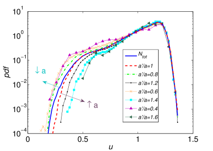
Figure 8: Probability density functions of particle streamwise (a) and wall-normal velocities (b), for $\sigma_{a}/(2a)=0.1$.

Concerning the $pdf$s of streamwise particle velocities, we see that the variance $\sigma_{u}^{2}$ increases as the particle radius is reduced, while it decreases for increasing $a^{\prime}$. In particular, the $pdf$s are identical for velocities higher than the modal value while the larger differences are found in the low velocity tails. Smaller particles are indeed able to closely approach the walls and hence translate with lower velocities than larger particles. Having in mind the profile of the mean streamwise velocity in a channel flow, it is then clear that larger particles whose centroids are more distant from the walls, translate more quickly than smaller particles.
The $pdf$s of the wall-normal velocities show less differences when varying $a^{\prime}$. The variance is similar for all species. One can however still notice that the variance slightly increases for smaller particles (smaller $a^{\prime}$) while it decreases for larger ones ( larger $a^{\prime}$). As discussed in the previous section, smaller particles have smaller Stokes numbers (i.e. smaller inertia) and are perturbed more easily by turbulence structures thereby reaching higher velocities (with higher probability) than larger particles.

Finally, we discuss the particles dispersion in the streamwise and spanwise directions. Particle motion is constrained in the wall-normal direction by the presence of the walls and is therefore not examined here. The dispersion is quantified as the variance of the particle displacement as function of the separation time $\Delta t$ (i.e. the mean-square displacement of particle trajectories)

$$\langle\Delta{\bf x}^{2}\rangle(\Delta t)=\langle\left[{\bf x}_{p}(\bar{t}+\Delta t)-{\bf x}_{p}(\bar{t})\right]^{2}\rangle_{p,\bar{t}}$$ (8)

where $\langle\cdot\rangle_{p,\bar{t}}$ denotes averaging over time $\bar{t}$ and the number of particles $p$.
The mean-square displacement in the streamwise direction is shown in figure 9$(a)$. From the subplot we see that initially, in the so-called ballistic regime, particle dispersion $\langle\Delta x^{2}\rangle$ shows a quadratic dependence on time. Only after $\Delta t\sim 100(2a)/U_{0}$ the curve starts to approach the linear behavior typical of a diffusive motion. As expected, we observe that smaller particles have a larger mean-square displacement than larger particles in the ballistic regime. However, the difference between $\langle\Delta{\bf x}^{2}\rangle$ for the smallest and largest particles ($a^{\prime}/a=0.4$ and $1.6$) is limited.

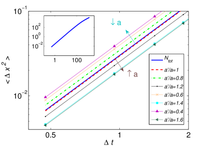
Figure 9: Mean-squared displacement of particles in the streamwise (a) and spanwise directions (b) for $\sigma_{a}/(2a)=0.1$.

Concerning the dispersion in the spanwise direction (figure 9$(b)$), we clearly notice that $\langle\Delta z^{2}\rangle$ is $1$ and $2$ orders of magnitude smaller than $\langle\Delta x^{2}\rangle$ in the ballistic and diffusive regimes. The latter is also reached earlier than in the streamwise direction, due to the absence of a mean flow. The discussion of the previous paragraph on the effect of particle size on dispersion in the ballistic regime, applies also in the present case. However, as the diffusive regime is approached, the mean-squared displacements $\langle\Delta z^{2}\rangle$ of all $a^{\prime}/a$ become more similar. For each $a^{\prime}/a$ we also find that the diffusion coeffient, defined as $D_{p,z}\simeq\langle\Delta z^{2}\rangle/(2\Delta t)$, is approximately $0.08$. A remarkable and not yet understood difference is found for $a^{\prime}/a=1.4$, for which $D_{p,z}$ is found to be $7\%$ larger. This could be due to the fact that less samples are used to calculate $\langle\Delta z^{2}\rangle$. The number of particles with $a^{\prime}/a=1.4$ is indeed substantially smaller than for $a^{\prime}/a\in[0.8;1.2]$.

To conclude this section, we emphasize that particle related statistics (probability density functions of velocities and mean-square displacements) only slightly vary for different $a^{\prime}/a$. In particular, the $pdf$s of particle velocities for smaller particles are wider than those of the larger particles. Accordingly, the mean-squared displacement $\langle\Delta{\bf x}^{2}\rangle$ of particles with $a^{\prime}/a<1$ is larger than that for particles with $a^{\prime}/a>1$, at least in the ballistic regime. Indeed, in the spanwise direction we find that the diffusion coeffients are approximately similar for all species.

III.2.1 Particle collision rates

We then study particle-pair statistics. In particular we calculate the radial distribution function $g(r)$ and the averaged normal relative velocity between two approaching particles, $\langle dv_{n}^{-}(r)\rangle$, and finally the collision kernel $\kappa(r)$ sundaram1997 .
The radial distribution function $g(r)$ is an indicator of the radial separation among particle pairs. In a reference frame with origin at the centre of a particle, $g(r)$ is the average number of particle centers located in the shell of radius $r$ and thickness $\Delta r$, normalized with the number of particles of a random distribution. Formally the $g(r)$ is defined as

$$g(r)=\frac{1}{4\pi}\frac{dN_{r}}{dr}\frac{1}{r^{2}n_{0}},$$ (9)

where $N_{r}$ is the number of particle pairs on a sphere of radius $r$, $n_{0}=N_{p}(N_{p}-1)/(2V)$ is the density of particle pairs in the volume $V$, with $N_{p}$ the number of particles. The value of $g(r)$ at distances of the order of the particle radius reveals the intensity of clustering; $g(r)$ tends to $1$ as $r\to\infty$, corresponding to a random (Poissonian) distribution. Here, we calculate it for pairs of particles with equal radii in the range $a^{\prime}/a\in[0.6;1.4]$, and among particles of different sizes ($a^{\prime}/a=0.8$ with $a^{\prime}/a=1.2$ and $a^{\prime}/a=0.6$ and $a^{\prime}/a=1.4$). For each case, the radial distance $r$ is normalized by $a^{\prime}$ or by the average between the radii of two approaching spheres. The radial distribution function is shown in figure 10$(a)$. No appreciable differences between each curve can be observed. The $g(r)$ is found to drop quickly to the value of the uniform distribution (i.e. 1) at $r\sim 2.5a^{\prime}$.
The normal relative velocity of a particle pair is instead obtained by projecting the relative velocity in the direction of the separation vector between the particles

$$dv_{n}(r_{ij})=({\bf u}_{i}-{\bf u}_{j})\cdot\frac{({\bf r}_{i}-{\bf r}_{j})}{|({\bf r}_{i}-{\bf r}_{j})|}=({\bf u}_{i}-{\bf u}_{j})\cdot\frac{{\bf r}_{ij}}{|{\bf r}_{ij}|}$$ (10)

(where $i$ and $j$ denote the two particles). This scalar quantity can be either positive (when two particles depart form each other) or negative (when they approach). Hence, the averaged normal relative velocity can be decomposed into $\langle dv_{n}(r)\rangle=\langle dv_{n}^{+}(r)\rangle+\langle dv_{n}^{-}(r)\rangle$. Here, we consider the absolute value of the mean negative normal relative velocity, shown in figure 10$(b)$. We observe that larger particles approach with a slightly larger relative velocity $\langle dv_{n}^{-}(r)\rangle$ than smaller particles. This could be explained by looking at the probability density functions of the streamwise particle velocities shown in figure 8$(a)$. From this we see indeed that smaller particles can experience lower velocities with non-negligible probability, in comparison to larger particles.

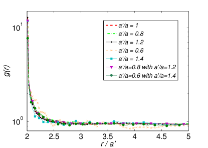
Figure 10: Radial distribution function $g(r)$ (a), average normal relative velocity $\langle dv_{n}^{-}\langle$ (b), collision kernel $\kappa(r)$ (c) and zoom of $\kappa(r)$ at contact (d), for $\sigma_{a}/(2a)=0.1$.

Finally, figures 10$(c),(d)$ report the collision kernel $\kappa(r)$ between particle-pairs. This is calculated as the product of the radial distribution function $g(r)$ and $\langle dv_{n}^{-}(r)\rangle$ sundaram1997 . At large seprataions, (i.e. $r/a^{\prime}>2.5$), we see that $\kappa(r)$ is fully dominated by the normal relative velocity. Around contact (i.e. $r/a^{\prime}\simeq 2$) we see clearly that $\kappa(r)$ is higher for larger particles, see figure 10$(d)$. The interesting result is found when looking at the collision kernels between particles of different sizes but equal concentration (within the suspension). For the case with $a^{\prime}/a=0.8$ and $a^{\prime}/a=1.2$, we see that $\kappa(r)$ is closer to that obtained for equal spheres with $a^{\prime}/a=0.8$. Also for the case with $a^{\prime}/a=0.6$ and $a^{\prime}/a=1.4$, we see that $\kappa(r)$ is similar to that obtained for equal spheres with $a^{\prime}/a=0.6$. This leads to the conclusion that collision statistics are dominated by the behavior of smaller particles.

IV Final remarks

We study numerically the behavior of monodisperse and polydisperse suspensions of rigid spheres in a turbulent channel flow. We consider suspensions with three different Gaussian distributions of particle radii (i.e. different standard deviations). The mean particle radius is equal to the reference radius of the monodisperse case. For the largest standard deviation, the ratio between largest and smallest particle radius is equal to $4$. We compare both fluid and particle statistics obtained for each case at a constant solid volume fraction $\phi=10\%$, hence, the total number of particles changes in each simulation.

The main finding of this work is that fluid and solid phase statistics for all polydisperse cases are similar to those obtained for the monodisperse suspension. This suggests that the key parameter in understanding the behavior of suspensions of rigid spheres in turbulent channel flows is the solid volume fraction $\phi$. Polydisperse suspensions with Gaussian distributions of particle sizes behave statistically in the same manner as a monodisperse suspension with equal volume fraction. This is probably not true for highly skewed size distributions.
Although results are similar, it is possible to observe small variations in the fluid and particle velocity fluctuations that are correlated to changes in the standard deviation $\sigma_{a}$ of the distribution. Concerning fluid velocity fluctuations we see that by increasing $\sigma_{a}$, these decrease at the centerline. The same is also found for particle velocity fluctuations. As $\sigma_{a}$ increases, larger particles are more likely found at the centerline and move almost unperturbed in the streamwise direction (hence also inducing smaller velocity fluctuations in the fluid phase). Particle velocity fluctuations are on the other hand found to increase with $\sigma_{a}$ close to the wall (in the viscous and buffer layers). This is probably related to the fact that for larger $\sigma_{a}$ smaller particles can penetrate more into this layer hence experiencing larger velocity fluctuations. Similar trends are observed for a smaller volume fraction of $2\%$.
Concerning the mean concentration of particles across the channel, we observe that the typical peak in proximity of the wall is smoothed for increasing $\sigma_{a}$. On the contrary, the mean concentration increases at the centerline at larger $\sigma_{a}$. Looking at the mean concentration profiles of each particle species (i.e. with different $a^{\prime}$), we observe that all particles are uniformly distributed. For particles smaller than the reference ones, the near-wall peak moves closer to the wall, while for larger particles the peak is moved away from the wall and is smoothed for increasing $a^{\prime}$.
We also calculated the Stokes number for each particles species. For the most extreme case, we found that there is an order of magnitude difference between $St_{a}^{\prime}$ of larger and smaller particles. However, the mean Stokes number of the suspension is the same as that of the reference particles (i.e. the same as well as that of the monodisperse case). Hence, suspensions with same volume fraction and mean Stokes number behave statistically in a similar way. If a skewed distribution of particles was used, the mean Stokes number would change and probably different results to the monodisperse ones would be observed. This may have important implications for the modeling of particulate flows in channels.
Then, we looked at probability density functions, $pdf$s, of particle velocities as well as particles mean-squared displacements for each species for the most extreme case with $\sigma_{a}/(2a)=0.1$. Concerning the $pdf$s of streamwise velocity, we notice that smaller particles can penetrate more in the layers closer to the walls and hence also experience smaller velocities (wider left tail of the $pdf$). The opposite is of course found for particles with larger $a^{\prime}$. The $pdf$s of wall-normal velocities are found to be extremely similar for all species, although the variance is just slightly increased for the smaller particles. This may be related to the fact that their Stokes number is smaller and hence they respond more quickly to velocity perturbations induced by turbulent eddies, hence reaching slightly larger velocities.
The mean-squared displacements of particles in the streamwise and spanwise directions, are similar for all species. Although larger particles are found to disperse less than smaller ones in the ballistic regime, the final diffusion coefficients are similar for all species. Finally, we studied particle-pair statistics by looking at the radial distribution function $g(r)$ and average normal relative velocity, $\langle dv_{n}^{-}(r)\rangle$, of approaching particles, as well as the resulting collision kernel, $\kappa(r)$. We found the interesting result that for pairs of particles with different sizes, the collision kernel $\kappa(r)$ is dominated by the behavior of smaller particles.

We have therefore shown that in turbulent channel flows, polydisperse suspensions with gaussian distributions of sizes behave similarly to monodisperse suspensions, provided that: the volume fraction is constant; the mean Stokes number of the suspension is the same as that of the monodispersed particles. On the other hand, particles of different size lead to non trivial particle-pair statistics.

References

References

- (1) J. J. Stickel, R. L. Powell, Fluid mechanics and rheology of dense suspensions, Annual Review of Fluid Mechanics 37 (2005) 129–149.
- (2) J. F. Morris, A review of microstructure in concentrated suspensions and its implications for rheology and bulk flow, Rheologica Acta 48 (8) (2009) 909–923.
- (3) N. J. Wagner, J. F. Brady, Shear thickening in colloidal dispersions, Physics Today 62 (10) (2009) 27–32.
- (4) E. Guazzelli, J. F. Morris, A physical introduction to suspension dynamics, Vol. 45, Cambridge University Press, 2011.
- (5) A. Einstein, Eine neue bestimmung der moleküldimensionen, Annalen der Physik 324 (2) (1906) 289–306.
- (6) A. Einstein, Berichtigung zu meiner arbeit:„eine neue bestimmung der moleküldimensionen” ̵︁, Annalen der Physik 339 (3) (1911) 591–592.
- (7) G. Batchelor, The stress system in a suspension of force-free particles, Journal of Fluid Mechanics 41 (03) (1970) 545–570.
- (8) P. Kulkarni, J. Morris, Suspension properties at finite reynolds number from simulated shear flow, Physics of Fluids 20 (040602).
- (9) F. Picano, W.-P. Breugem, D. Mitra, L. Brandt, Shear thickening in non-brownian suspensions: an excluded volume effect, Physical Review Letters 111 (9) (2013) 098302.
- (10) J. F. Morris, H. Haddadi, Microstructure and rheology of finite inertia neutrally buoyant suspensions, Journal of Fluid Mechanics 749 (2014) 431–459.
- (11) W. Fornari, L. Brandt, P. Chaudhuri, C. U. Lopez, D. Mitra, F. Picano, Rheology of confined non-brownian suspensions, Physical Review Letters 116 (1) (2016) 018301.
- (12) R. A. Bagnold, Experiments on a gravity-free dispersion of large solid spheres in a newtonian fluid under shear, in: Proceedings of the Royal Society of London A: Mathematical, Physical and Engineering Sciences, Vol. 225, The Royal Society, 1954, pp. 49–63.
- (13) J.-P. Matas, J. F. Morris, E. Guazzelli, Transition to turbulence in particulate pipe flow, Physical Review Letters 90 (1) (2003) 014501.
- (14) Z. Yu, T. Wu, X. Shao, J. Lin, Numerical studies of the effects of large neutrally buoyant particles on the flow instability and transition to turbulence in pipe flow, Physics of Fluids (1994-present) 25 (4) (2013) 043305.
- (15) I. Lashgari, F. Picano, L. Brandt, Transition and self-sustained turbulence in dilute suspensions of finite-size particles, Theoretical and Applied Mechanics Letters.
- (16) V. Loisel, M. Abbas, O. Masbernat, E. Climent, The effect of neutrally buoyant finite-size particles on channel flows in the laminar-turbulent transition regime, Physics of Fluids (1994-present) 25 (12) (2013) 123304.
- (17) I. Lashgari, F. Picano, W.-P. Breugem, L. Brandt, Laminar, turbulent, and inertial shear-thickening regimes in channel flow of neutrally buoyant particle suspensions, Physical Review Letters 113 (25) (2014) 254502.
- (18) S. Balachandar, J. K. Eaton, Turbulent dispersed multiphase flow, Annual Review of Fluid Mechanics 42 (2010) 111–133.
- (19) M. Reeks, The transport of discrete particles in inhomogeneous turbulence, Journal of aerosol science 14 (6) (1983) 729–739.
- (20) A. Soldati, C. Marchioli, Physics and modelling of turbulent particle deposition and entrainment: Review of a systematic study, International Journal of Multiphase Flow 35 (9) (2009) 827–839.
- (21) G. Sardina, F. Picano, P. Schlatter, L. Brandt, C. M. Casciola, Large scale accumulation patterns of inertial particles in wall-bounded turbulent flow, Flow, turbulence and combustion 86 (3-4) (2011) 519–532.
- (22) G. Sardina, P. Schlatter, L. Brandt, F. Picano, C. Casciola, Wall accumulation and spatial localization in particle-laden wall flows, Journal of Fluid Mechanics 699 (2012) 50–78.
- (23) J. D. Kulick, J. R. Fessler, J. K. Eaton, Particle response and turbulence modification in fully developed channel flow, Journal of Fluid Mechanics 277 (1) (1994) 109–134.
- (24) L. Zhao, H. I. Andersson, J. Gillissen, Turbulence modulation and drag reduction by spherical particles, Physics of Fluids (1994-present) 22 (8) (2010) 081702.
- (25) Y. Pan, S. Banerjee, Numerical simulation of particle interactions with wall turbulence, Physics of Fluids (1994-present) 8 (10) (1996) 2733–2755.
- (26) A. G. Kidanemariam, C. Chan-Braun, T. Doychev, M. Uhlmann, Direct numerical simulation of horizontal open channel flow with finite-size, heavy particles at low solid volume fraction, New Journal of Physics 15 (2) (2013) 025031.
- (27) X. Shao, T. Wu, Z. Yu, Fully resolved numerical simulation of particle-laden turbulent flow in a horizontal channel at a low reynolds number, Journal of Fluid Mechanics 693 (2012) 319–344.
- (28) F. Picano, W.-P. Breugem, L. Brandt, Turbulent channel flow of dense suspensions of neutrally buoyant spheres, Journal of Fluid Mechanics 764 (2015) 463–487.
- (29) P. Costa, F. Picano, L. Brandt, W.-P. Breugem, Universal scaling laws for dense particle suspensions in turbulent wall-bounded flows, Physical Review Letters 117 (13) (2016) 134501.
- (30) A. Prosperetti, Life and death by boundary conditions, Journal of Fluid Mechanics 768 (2015) 1–4.
- (31) W. Fornari, A. Formenti, F. Picano, L. Brandt, The effect of particle density in turbulent channel flow laden with finite size particles in semi-dilute conditions, Physics of Fluids (1994-present) 28 (3) (2016) 033301.
- (32) M. N. Ardekani, P. Costa, W.-P. Breugem, F. Picano, L. Brandt, Drag reduction in turbulent channel flow laden with finite-size oblate spheroids, arXiv preprint arXiv:1607.00679.
- (33) W.-P. Breugem, A second-order accurate immersed boundary method for fully resolved simulations of particle-laden flows, Journal of Computational Physics 231 (13) (2012) 4469–4498.
- (34) T. Kempe, J. Fröhlich, An improved immersed boundary method with direct forcing for the simulation of particle laden flows, Journal of Computational Physics 231 (9) (2012) 3663–3684.
- (35) H. Brenner, The slow motion of a sphere through a viscous fluid towards a plane surface, Chemical Engineering Science 16 (3) (1961) 242–251.
- (36) D. Jeffrey, Low-reynolds-number flow between converging spheres, Mathematika 29 (1982) 58–66.
- (37) R. A. Lambert, F. Picano, W.-P. Breugem, L. Brandt, Active suspensions in thin films: nutrient uptake and swimmer motion, Journal of Fluid Mechanics 733 (2013) 528–557.
- (38) W. Fornari, F. Picano, L. Brandt, Sedimentation of finite-size spheres in quiescent and turbulent environments, Journal of Fluid Mechanics 788 (2016) 640–669.
- (39) L. Schiller, A. Naumann, A drag coefficient correlation, Vdi Zeitung 77 (318) (1935) 51.
- (40) S. Sundaram, L. R. Collins, Collision statistics in an isotropic particle-laden turbulent suspension. part 1. direct numerical simulations, Journal of Fluid Mechanics 335 (1997) 75–109.