Boost invariant formulation of the chiral kinetic theory

Abstract

We formulate the chiral kinetic equation with the longitudinal boost invariance. We particularly focus on the physical interpretation of the particle number conservation. There appear two terms associated with the expansion, which did not exist in the non-chiral kinetic equation. One is a contribution to the transverse current arising from the side-jump effect, and the other is a change in the density whose flow makes the longitudinal current. We point out a characteristic pattern in the transverse current driven by the expansion, which we call the chiral circular displacement.

I Introduction

In theoretical and experimental research on relativistic heavy-ion collisions and also condensed matter systems of Weyl/Dirac semimetals chiral matter with massless fermionic dispersions has been attracting more and more interest. The most notable features in chiral matter are exotic phenomena driven by chirality and quantum anomaly such as the Chiral Magnetic Effect (CME) Kharzeev et al. (2008); Fukushima et al. (2008); the CME is realized as an electric current along the external magnetic field in the presence of imbalanced chiral charge (see recent reviews Kharzeev et al. (2016); Hattori and Huang (2017) for more details). The CME physics has triggered various theoretical investigations including the anomalous hydrodynamics with chiral anomaly Son and Surowka (2009); Sadofyev and Isachenkov (2011); Pu et al. (2011), lattice numerical simulations of quantum chromodynamics (QCD) with a chiral chemical potential Abramczyk et al. (2009); Buividovich et al. (2009a, b, 2010); Yamamoto (2011), holographic models based on gauge/gravity correspondence Erdmenger et al. (2009); Torabian and Yee (2009); Banerjee et al. (2011), the quantum kinetic description with Wigner functions Gao et al. (2012, 2017), and the kinetic theory with the Berry curvature Son and Yamamoto (2012, 2013); Stephanov and Yin (2012); Chen et al. (2013).

In non-central heavy-ion collisions, a magnetic field as strong as the QCD energy scales is expected; see e.g. Ref. Skokov et al. (2009) for the first estimate using the Ultrarelativistic Quantum Molecular Dynamics (UrQMD) model, Refs. Bzdak and Skokov (2012); Deng and Huang (2012); Roy and Pu (2015) for even-by-event simulations, and Refs. Tuchin (2015); Li et al. (2016) for the case with finite chiral conductivity. Moreover, with imbalanced chirality induced from the topological transition on P- and CP-violating gauge backgrounds, the CME currents are anticipated to generate the charge asymmetry fluctuations as measured first in the STAR Collaboration Abelev et al. (2009, 2010). To distinguish the genuine signal from flow backgrounds, quantitative studies are indispensable. Besides, some other novel effects from chiral transport may also play a substantial role in quantitative simulations for the heavy-ion collisions, e.g. the chiral electric separation effect Huang and Liao (2013); Pu et al. (2014), the chiral Hall separation effect Gursoy et al. (2014); Pu et al. (2015), and higher order effects Chen et al. (2016); Gorbar et al. (2016).

For real-time simulations of the CME, three approaches are commonly adopted. The first one is the classical statistical simulation based on the solution of the classical Yang-Mills and Dirac equations; see Refs. Mace et al. (2016, 2017); Berges et al. (2017) for recent studies. The second is the anomalous hydrodynamics or the chiral magneto-hydrodynamics (CMHD), see Ref. Hirono et al. (2014); Jiang et al. (2016) for recent studies and also Refs. Roy et al. (2015); Pu et al. (2016) for the analytic one-dimensional solutions, Ref. Pu and Yang (2016) for the two-dimensional Bjorken expanding case, and Ref. Inghirami et al. (2016) for more simulations.

When the occupation number is dilute, the third and the most microscopic approach becomes feasible, i.e. the kinetic theory that can be applied for general systems out of equilibrium. The conventional Boltzmann equation is not capable of treating the spin dynamics Pu et al. (2011) and the kinetic theory augmented with the spin dynamics for chiral matter is called the chiral kinetic theory (CKT) Son and Yamamoto (2012, 2013); Stephanov and Yin (2012); Chen et al. (2013). See also Refs. Sun et al. (2016); Huang et al. (2017) for latest CKT simulations. To derive the equations of motion for the spin, the Berry curvature Berry (1984) should be added to the action in the path-integral formulation (see Refs. Xiao et al. (2005); Duval et al. (2006) for discussions and Ref. Xiao et al. (2010) for a review). In this way the Berry curvature corrections are expected to the Boltzmann equation, as was concluded in Refs. Son and Yamamoto (2012, 2013); Stephanov and Yin (2012); Chen et al. (2013, 2014a, 2014b); Hidaka et al. (2017).

To consider the early stage of the time evolution in the relativistic heavy-ion collision, the Boltzmann equation in expanding geometry has played an essential role. One of the earliest applications is found in the explanation of the isotropization mechanism in the relaxation time approximation Baym (1984). The QCD interaction was taken into account in Ref. Mueller (2000), which is the foundation for the bottom-up thermalization scenario Baier et al. (2001) (see Ref. Fukushima (2017) for a recent review and references therein). So far, most of preceding works have been focused on the gluonic sector called “glasma” (see Refs. Fukushima (2017); Blaizot (2017) for pedagogical reviews on the gluon saturation and the glasma picture) because the early time dynamics is dominated by gluonic degrees of freedom due to quantum evolution. Here, let us point out advantages to consider the quark sector.

The first important feature in the quark sector is that, unlike gluons, physical conditions validate the kinetic description for quarks. The reason why the quantum Boltzmann equation  cannot be utilized in the glasma regime is that the gluons are overpopulated and the non-linearity must be fully taken into account. In contrast, quarks are never overpopulated since they obey the Fermi statistics.

The second is that the quark distribution in the very early stage of the heavy-ion collision should be dilute, so that the dominant process should be the interaction between quarks and background gluonic fields. Thus, even in an approximation to neglect the collision integral, the CKT can correctly capture the quark dynamics, and nevertheless, the results are non-trivial as revealed in this paper.

The third is that, in the non-central collision, the strong external magnetic field quickly decays, but it can survive over the time scale of the glasma that may accommodate the topological charge fluctuations Kharzeev et al. (2002); Mace et al. (2016). Such a combination of the magnetic and the gluonic fields would yield visible effects of the local parity violation. For the sake of investigating this, the CKT provides us with a powerful and microscopic tool, and in principle, we should be able to estimate physical observables from the glasma-type initial condition.

There is an obstacle, however. Although the CKT itself has been established, it is far from straightforward to apply the CKT to the heavy-ion phenomenology since the realization of the Lorentz symmetry in chiral matter is highly non-trivial Chen et al. (2014b, 2015). Under the Lorentz boost, usually, the coordinate vector $\boldsymbol{x}$ and the momentum vector $\boldsymbol{p}$ as well as the electromagnetic fields should transform as vectors and tensors, but it has been found in Refs. Chen et al. (2014b, 2015) that transformed $\boldsymbol{x}$ and $\boldsymbol{p}$ must have extra terms of order of the Berry curvature, which are called side-jump effects Chen et al. (2014b). One can reach the same conclusion by looking at the classical effective action of chiral matter. Later, from the quantum field theoretical formulation, it has been demonstrated in Ref. Hidaka et al. (2017) that, instead of elaborating $\boldsymbol{x}$ and $\boldsymbol{p}$ transformations, a non-trivial transformation on the distribution function under the Lorentz boost can lead to equivalent consequences Chen et al. (2015).

The question that we would like to address in this work is; what is the counterpart of the boost invariant Boltzmann equation of Refs. Baym (1984); Mueller (2000) for quarks? For clarity let us make two remarks here. (1) One might think that the boost invariance makes the topology of theory trivial. This is completely true, and the topological charge is vanishing Kharzeev et al. (2002); however, the topological charge density can distribute over space, which is nothing but a microscopic picture of the local parity violation. (2) Also, one might think that the boost invariance is anyway broken by quantum fluctuations. This is indeed so in the gluonic sector that exhibits the glasma instability Romatschke and Venugopalan (2006) but not true in the quark sector. As long as the time scale is shorter than the glasma instability growth (i.e. up to a few times the saturation momentum inverse), we can treat glasma fields as boost invariant gluonic backgrounds. Also, the spatial variations of the external magnetic field spread more smoothly than the saturation scale, and so we can again regard the magnetic field as approximately boost invariant. Then, one can prove that the mode functions in the quark sector keep boost invariance as long as external fields have no dependence on the coordinate rapidity Gelis et al. (2005); Gelis and Tanji (2016).

More specifically, spinors as solutions of the Dirac equation explicitly have boost invariant properties once the spinor components are appropriately transformed in the co-moving frame. Therefore, naturally, the quark distribution function appearing in the CKT must share the same properties because the distribution function is microscopically defined in terms of the solutions of the Dirac equation. Then, with the boost invariant Ansatz for the distribution function, the CKT is rewritten in a way that makes the expansion effect manifested.

The organization of the present paper is as follows; in Sec. II we discuss the Dirac equation and the boost invariance following the discussions in Ref. Gelis and Tanji (2016). In Sec. III we then briefly review what is known for the ordinary Boltzmann equation with the boost invariant Ansatz for the distribution function. We proceed to Sec. IV to discuss the application of the CKT to the system with boost invariance, which is followed by some considerations on the non-trivial realization of the particle number conservation in Sec. V. Finally, we make a summary in Sec. VI.

II Dirac equation with boost invariance

Let us first consider the Dirac equation under external electromagnetic fields. The generalization to non-Abelian fields should be straightforward. Throughout this work we always assume boost invariant electromagnetic fields, which is the case in the CGC-type chromo-fields for instance. It is useful to rewrite the equation of motion in terms of the Bjorken coordinates, namely, the proper time, $\tau\equiv\sqrt{t^{2}-z^{2}}$, and the coordinate rapidity, $\eta\equiv\frac{1}{2}\ln|(t-z)/(t+z)|$. Then, boost invariance is translated into the $\eta$ independence of external fields. We can also introduce the momentum counterparts, that is, the transverse momentum, $p_{\perp}\equiv\sqrt{p_{0}^{2}-p_{z}^{2}}$, and the momentum rapidity, $y\equiv\frac{1}{2}\ln|(p_{0}-p_{z})/(p_{0}+p_{z})|$.

The limit of vanishing external fields is the simplest example that is useful for our consideration. Needless to say, the solution of the equation of motion is then a plane wave, $e^{ip\cdot x}$, apart from the spinor components. Actually, using the Bjorken coordinates, we can express the (longitudinal part of) plane wave as $e^{\mp i(p_{0}x^{0}+p_{z}z)}=e^{\mp ip_{\perp}\tau\cosh(y-\eta)}$. In this way, we understand that the Lorentz invariance requires a special combination of rapidity dependence through $y-\eta$ only. Now, with interactions introduced in the covariant derivative, the massless Dirac equation reads Gelis et al. (2005),

$$i\biggl{(}\gamma^{0}\partial_{\tau}+\frac{\gamma^{0}}{2\tau}+\frac{\gamma^{z}}{\tau}D_{\eta}+\gamma^{i}D_{i}\biggr{)}\tilde{\psi}=0\;,$$ (1)

where $\tilde{\psi}=e^{-\frac{\eta}{2}\gamma^{0}\gamma^{z}}\psi$ and the $A_{\tau}=0$ gauge is chosen. We can even simplify the above by changing the fermion basis as $\tilde{\psi}\to\hat{\psi}=\tau^{1/2}\tilde{\psi}$ yielding Gelis and Tanji (2016),

$$i\biggl{(}\gamma^{0}\partial_{\tau}+\frac{\gamma^{z}}{\tau}D_{\eta}+\gamma^{i}D_{i}\biggr{)}\hat{\psi}=0\;.$$ (2)

As long as there is no $\eta$ dependence in gauge potentials, we can now explicitly solve the $\eta$ dependence for particles and anti-particles by plugging $e^{\mp ip_{\perp}\tau\cosh(y-\eta)}\chi_{\mp}$ for $\hat{\psi}$ into the Dirac equation, and we then find for the right-handed two-spinor part for example;

$$\biggl{(}\partial_{\tau}\mp ip_{\perp}e^{-\sigma^{3}(y-\eta)}+i\frac{\sigma^{3}}{\tau}gA_{\eta}+\sigma^{i}D_{i}\biggr{)}\chi_{\mp}^{R}(\tau,\boldsymbol{x}_{T};y-\eta)=0\;.$$ (3)

Here, the rapidity dependence appears only in the second term of the equation of motion, and obviously, the time evolution maintains the boost invariant property; a complete set of wave-functions are functions of $y-\eta$ for any $\tau$. Therefore, naturally, the distribution function that is to be defined by wave-functions must be also a function of $y-\eta$.

It is crucially important to notice that, when we talk about the boost invariance of physical states, we mean their dependence through $y-\eta$, while we assume $\eta$ independence for external fields.

III Boltzmann equation with boost invariance

As a preliminary exercise for the CKT formulation with boost invariance, let us make a brief review on the ordinary Boltzmann equation following Ref. Mueller (2000). The Boltzmann equation or the Vlasov equation reads,

$$\frac{\partial}{\partial t}f+\boldsymbol{v}\cdot\frac{\partial}{\partial\boldsymbol{x}}f+(\boldsymbol{E}+\boldsymbol{v}\times\boldsymbol{B})\cdot\frac{\partial}{\partial\boldsymbol{p}}f=I_{{\rm coll}}[f]\;,$$ (4)

where $f(\boldsymbol{p},\boldsymbol{x},t)$ is the distribution function in phase space, and $\boldsymbol{E}$, $\boldsymbol{B}$ are electromagnetic fields. The velocity is defined by $\boldsymbol{v}\equiv\partial\varepsilon_{p}/\partial\boldsymbol{p}$ with $\varepsilon_{p}=|\boldsymbol{p}|$. In what follows below we will neglect the external fields for simplicity.

If we impose boost invariance along the longitudinal (i.e. $z$) direction, such a condition restricts the form of the distribution function as $f(\boldsymbol{p},\boldsymbol{x},t)=f(\boldsymbol{p}_{\perp},\boldsymbol{x}_{\perp},y-\eta,\tau)$. This implies that the following relations should hold;

$$\frac{\partial f}{\partial t}=\biggl{(}\frac{t}{\tau}\frac{\partial}{\partial\tau}+\frac{z}{\tau^{2}}\frac{\partial}{\partial\eta}\biggr{)}f\;,$$ (5)

and

$$\frac{\partial f}{\partial z}=\biggl{(}-\frac{z}{\tau}\frac{\partial}{\partial\tau}-\frac{t}{\tau^{2}}\frac{\partial}{\partial\eta}\biggr{)}f\;.$$ (6)

Using the velocity vector, $v_{x}=v_{y}=0$ and $v_{z}=p_{z}/p_{0}$, we can readily see,

$$\biggl{(}\frac{\partial}{\partial t}+v_{z}\frac{\partial}{\partial z}\biggr{)}f=\frac{\cosh(y-\eta)}{\cosh y}\biggl{(}\frac{\partial}{\partial\tau}-\frac{\tanh(y-\eta)}{\tau}\frac{\partial}{\partial y}\biggr{)}f\;,$$ (7)

where we used $\partial f/\partial\eta=-\partial f/\partial y$. Here, again, we see that the time evolution of the Boltzmann equation preserves the dependence only through $y-\eta$, apart from the overall (trivially factorizable) $y$ dependence.

It is a common strategy to consider only around the mid-rapidity region, i.e. $\eta\approx 0$ and $z\approx 0$, to simplify the equations as

$$\biggl{(}\frac{\partial}{\partial t}+v_{z}\frac{\partial}{\partial z}\biggr{)}f\approx\biggl{(}\frac{\partial}{\partial t}-\frac{p_{z}}{t}\frac{\partial}{\partial p_{z}}\biggr{)}f\;.$$ (8)

We note that the above prescription does not mean that we are looking at a single point $z=0$ but we make a systematic expansion in $z$ around $z=0$ to pick up leading terms.

Now we can easily develop intuitive understanding for the second term in the above as follows. Let us take the momentum integration to find an equation for the density defined by $n(\boldsymbol{x})\equiv\int_{\boldsymbol{p}}f(\boldsymbol{p},\boldsymbol{x})$. After the integration by part with respect to $p_{z}$, we find,

$$\frac{\partial n}{\partial t}+\frac{n}{t}+\boldsymbol{\nabla}_{\boldsymbol{x}_{\perp}}\cdot\boldsymbol{j}_{\perp}=0\;,$$ (9)

where the current term should result from the other parts in the Boltzmann equation and the collision integral is assumed to conserve the particle number. We can actually rewrite this into a form that will turn out to be convenient for later discussions;

$$\frac{\partial n}{\partial t}+\frac{\partial}{\partial z}\biggl{(}\frac{z}{t}n\biggr{)}+\boldsymbol{\nabla}_{\boldsymbol{x}_{\perp}}\cdot\boldsymbol{j}_{\perp}=0\;,$$ (10)

for $z\approx 0$. Here, $z/t$ is a velocity associated with longitudinal expansion, and thus, $(z/t)n$ gives a longitudinal current associated with boost invariant expansion.

So far we have considered the situation without electromagnetic fields for simplicity, the presence of $\boldsymbol{E}$ and $\boldsymbol{B}$ would result in the same structure of the continuity equation as Eq. (10). In the case of the ordinary Boltzmann equation with $\boldsymbol{E}$ and $\boldsymbol{B}$, the Lorentz form terms $\propto\boldsymbol{E}+\boldsymbol{v}\times\boldsymbol{B}$ are just surface terms and become vanishing after the momentum integration.

An external electric field should accelerate charged particles, so one might worry about the fate of boost invariance, though it should exist formally as argued in Sec. II. We shall than take a trivial example to deepen our insight here, that is, the ideal magneto-hydrodynamics Roy et al. (2015); Pu et al. (2016). By construction of the ideal magneto-hydrodynamics, the electric conductivity is taken to be infinite, and the electromagnetic force satisfies $\boldsymbol{E}+\boldsymbol{v}\times\boldsymbol{B}=0$, which means no force, and thus, no acceleration of charged particles. Naturally, the boost invariance is intact, which addresses another evidence for the existence of boost invariant states.

IV Extension to the Chiral Kinetic Theory

We shall treat the CKT under the same Ansatz for the distribution function with boost invariance. The CKT for right-handed particles is Stephanov and Yin (2012); Son and Yamamoto (2012, 2013); Chen et al. (2013); Hidaka et al. (2017)

$$(1+\boldsymbol{B}\cdot\boldsymbol{\Omega})\frac{\partial f}{\partial t}+\bigl{[}\boldsymbol{v}_{p}+(\boldsymbol{v}_{p}\cdot\boldsymbol{\Omega})\boldsymbol{B}+\boldsymbol{E}\times\boldsymbol{\Omega}\bigr{]}\cdot\frac{\partial f}{\partial\boldsymbol{x}}$$

$$+\bigl{[}\boldsymbol{E}+\boldsymbol{v}_{p}\times\boldsymbol{B}+(\boldsymbol{E}\cdot\boldsymbol{B})\boldsymbol{\Omega}\bigr{]}\cdot\frac{\partial f}{\partial\boldsymbol{p}}=I_{\rm coll}[f]\;,$$ (11)

where $\boldsymbol{\Omega}\equiv\hbar\boldsymbol{p}/(2|\boldsymbol{p}|^{3})$ is the Berry curvature, $\boldsymbol{v}_{p}\equiv\partial\varepsilon_{p}/\partial\boldsymbol{p}$ is the group velocity with the quasi-particle dispersion relation, $\varepsilon_{p}=|\boldsymbol{p}|(1-\boldsymbol{B}\cdot\boldsymbol{\Omega})$ (for the case of spatial homogeneity), and $I_{\rm coll}[f]$ is the collision integral. In this paper we will focus on the $I_{\rm coll}[f]=0$ case, assuming that the quark distribution is dilute in the early time dynamics of the heavy-ion collision.

Before we start our discussion, it would be instructive to explain more about the chiral anomaly and the boost invariance. As carefully worked out in Ref. Kharzeev et al. (2002), with boost invariance, there is no large gauge transformation that changes the Chern number $\nu$ due to trivial homotopy. Then, if the initial $\nu$ is vanishing, $\nu$ is always zero, and the winding number, $Q_{w}=\nu(\tau=\infty)-\nu(\tau=-\infty)$, is also trivial. However, this does not mean that the CKT with boost invariance is trivial. We usually consider the CKT for given gauge backgrounds. One may then consider some gauge configurations not necessarily given by the solutions of the equations of motion. A simple example of constant (and thus boost invariant) electromagnetic $\boldsymbol{E}\cdot\boldsymbol{B}$ can actually make $Q_{w}$ as large as one likes, irrespective to the homotopy.

As mentioned already in Sec. III we limit ourselves to deal with a region with $\eta\approx 0$ and $z\approx 0$. A rather superficial but controversial difficulty in this case is the appearance of the Berry curvature that also involves $p_{z}$ and it seemingly violates the dependence through $y-\eta$ only. However, as argued in the previous sections, the Lorentz invariance immediately concludes such functional dependence through $y-\eta$; it would be an intriguing theoretical problem to confirm this $y-\eta$ dependence explicitly for arbitrary $\eta$ and $z$. In this work, we take a more pragmatic strategy as follows. We now anticipate that the distribution function $f$ be a function of $y-\eta$, which is what we mean by boost invariance; $f$ itself is invariant under simultaneous shifts in $y$ and $\eta$. This requirement would provide us with a relation like Eq. (8), so that we can discuss a continuity relation analogously to Eqs. (9) and (10).

The correct boost transformation onto the CKT is known up to $\mathcal{O}(\hbar)$ as $\delta t=\boldsymbol{\beta}\cdot\boldsymbol{x}$, $\delta\boldsymbol{x}=\boldsymbol{\beta}t+\boldsymbol{\beta}\times p\boldsymbol{\Omega}$, $\delta\boldsymbol{p}=\boldsymbol{\beta}\varepsilon_{p}+(\boldsymbol{\beta}\times p\boldsymbol{\Omega})\times\boldsymbol{B}$, where $p=|\boldsymbol{p}|$ Chen et al. (2014b). The electromagnetic fields should transform as ordinarily as $\delta\boldsymbol{B}=\boldsymbol{\beta}\times\boldsymbol{E}$ and $\delta\boldsymbol{E}=-\boldsymbol{\beta}\times\boldsymbol{B}$ up to this order.

Under our treatment of the problem near $z\approx 0$ we can retain the leading terms in the expansion of small $\delta z$ around $z=0$ or small boost parameter $\boldsymbol{\beta}=-(\delta z/t)\boldsymbol{e}_{z}$. The boost transformation then reads,

$$\delta\boldsymbol{x} =-\delta z\,\boldsymbol{e}_{z}-\frac{\delta z}{t}\boldsymbol{e}_{z}\times p\boldsymbol{\Omega}\;,$$ (12)

$$\delta\boldsymbol{p} =-\delta z\frac{p}{t}\bigl{(}1-2\boldsymbol{B}\cdot\boldsymbol{\Omega}\bigr{)}\boldsymbol{e}_{z}-\delta z\frac{p}{t}B_{z}\boldsymbol{\Omega}\;,$$ (13)

up to the linear order in $\delta z$ and in $\boldsymbol{\Omega}$. The additional terms in $\boldsymbol{x}$ and $\boldsymbol{p}$ proportional to $\boldsymbol{\Omega}$ are often referred to as the side-jump terms. We note that there is a way to formulate the Lorentz transformation with side-jump terms incorporated not in $\boldsymbol{x}$ and $\boldsymbol{p}$ but in $f$ as discussed in Refs. Chen et al. (2015); Hidaka et al. (2017), and we have checked that both formulations eventually yield the same answer. The similar procedures to obtain Eq. (8) replace the $z$ dependence with the $p_{z}$ dependence, which immediately follows from $f(\boldsymbol{p},\boldsymbol{x},t)=f(\boldsymbol{p}+\delta\boldsymbol{p},\boldsymbol{x}+\delta\boldsymbol{x},t)$. The explicit form of the relation is

$$\begin{split}\frac{\partial f}{\partial z}&=-\frac{B_{z}p}{t}\boldsymbol{\Omega}\cdot\frac{\partial f}{\partial\boldsymbol{p}}-\frac{p}{t}\bigl{(}1-2\boldsymbol{B}\cdot\boldsymbol{\Omega}\bigr{)}\frac{\partial f}{\partial p_{z}}\\ &\qquad-\frac{p}{t}(\boldsymbol{e}_{z}\times\boldsymbol{\Omega})_{\perp}\cdot\frac{\partial f}{\partial\boldsymbol{x}_{\perp}}\;.\end{split}$$ (14)

We then plug the above into the original CKT and drop $\mathcal{O}(\hbar^{2})$ terms. We finally arrive at the following expression;

$$(1+\boldsymbol{B}\cdot\boldsymbol{\Omega})\frac{\partial f}{\partial t}+\biggl{[}(1+2\boldsymbol{B}\cdot\boldsymbol{\Omega})\hat{\boldsymbol{p}}+\boldsymbol{E}\times\boldsymbol{\Omega}$$

$$\quad-\frac{p_{z}}{t}\,\boldsymbol{e}_{z}\times\boldsymbol{\Omega}\biggr{]}_{\perp}\cdot\frac{\partial f}{\partial\boldsymbol{x}_{\perp}}+\biggl{[}\boldsymbol{E}+(1+2\boldsymbol{B}\cdot\boldsymbol{\Omega})\hat{\boldsymbol{p}}\times\boldsymbol{B}$$

$$\quad+(\boldsymbol{E}\cdot\boldsymbol{B})\boldsymbol{\Omega}-\frac{B_{z}p_{z}}{t}\boldsymbol{\Omega}$$

$$\quad-\frac{p}{t}\bigl{[}\hat{p}_{z}+(\boldsymbol{E}\times\boldsymbol{\Omega})_{z}\bigr{]}\boldsymbol{e}_{z}\biggr{]}\cdot\frac{\partial f}{\partial\boldsymbol{p}}=0\;.$$ (15)

It is easy to confirm that this kinetic equation reduces to the well-known form of Eq. (8) in the $\boldsymbol{\Omega}\to 0$ limit. This Eq. (15) is the central result in this paper.

V Particle Number Conservation

It may not be easy to grasp the physical meaning of the result (15). To make the physical meaning more accessible, let us address the continuity equation specifically here, which is obtained from the zeroth moment of the kinetic equation in general. The definition of the particle number density is slightly modified by the Berry curvature correction as Xiao et al. (2005)

$$n\equiv\int_{\boldsymbol{p}}(1+\boldsymbol{B}\cdot\boldsymbol{\Omega})f\;,$$ (16)

and then the momentum integration of Eq. (15) leads to

$$\frac{\partial n}{\partial t}+\frac{\tilde{n}}{t}+\boldsymbol{\nabla}_{\perp}\cdot\tilde{\boldsymbol{j}}_{\perp}=\frac{\boldsymbol{E}\cdot\boldsymbol{B}}{(2\pi\hbar)^{2}}f(\boldsymbol{p}=0)\;,$$ (17)

for constant $\boldsymbol{E}$ and $\boldsymbol{B}$, where the right-hand side is the chiral anomaly, and we defined the modified density and the modified transverse current as

$$\tilde{n}\equiv n-\int_{\boldsymbol{p}}\bigl{[}2\hat{p}_{z}(\boldsymbol{E}\times\boldsymbol{\Omega})_{z}+\boldsymbol{B}_{\perp}\cdot\boldsymbol{\Omega}_{\perp}\bigr{]}f\;,$$ (18)

and

$$\tilde{\boldsymbol{j}}_{\perp}\equiv\int_{\boldsymbol{p}}\Bigl{[}(1+2\boldsymbol{B}\cdot\boldsymbol{\Omega})\hat{\boldsymbol{p}}+\boldsymbol{E}\times\boldsymbol{\Omega}-\frac{p_{z}}{t}\,\boldsymbol{e}_{z}\times\boldsymbol{\Omega}\Bigr{]}_{\perp}f\;.$$ (19)

We note that the third term in $\tilde{\boldsymbol{j}}_{\perp}$, i.e. $-\int_{\boldsymbol{p}}(p_{z}/t)(\boldsymbol{e}_{z}\times\boldsymbol{\Omega})_{\perp}f$, arises from the side-jump effects in $\boldsymbol{x}$ referring to $\delta\boldsymbol{x}$ in Eq. (12). The appearance of such an additional transverse current is peculiar in the longitudinally expanding situation, while the other terms in $\tilde{\boldsymbol{j}}_{\perp}$ are just standard ones in the CKT Stephanov and Yin (2012); Son and Yamamoto (2012, 2013); Chen et al. (2013); Hidaka et al. (2017). We also note that those additional terms in $\tilde{\boldsymbol{j}}_{\perp}$ as well as those in $\tilde{n}$ are non-vanishing only when $f$ has an anisotropic distribution in momentum space.

It is useful to write the continuity equation in a way similar to Eq. (10), that is, from Eq. (17) we have,

$$\frac{\partial n}{\partial t}+\frac{\partial}{\partial z}\biggl{(}\frac{z}{t}\tilde{n}\biggl{)}+\boldsymbol{\nabla}_{\perp}\cdot\tilde{\boldsymbol{j}}_{\perp}=\frac{\boldsymbol{E}\cdot\boldsymbol{B}}{(2\pi\hbar)^{2}}f(\boldsymbol{p}=0)\;,$$ (20)

for $z\approx 0$. Then, $(z/t)\tilde{n}$ represents a current associated with the longitudinally expanding medium. Importantly, here, the density corresponding to this longitudinal current is not characterized by $n$ itself but $\tilde{n}$, modified by the Berry curvature as in Eq. (18).

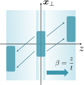
Figure 1: Schematic figure to explain how the shift takes place.

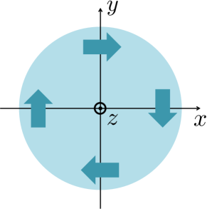
Figure 2: Schematic figure to show the characteristic shift pattern seen from the transverse plane for $z>0$.

Even without external electromagnetic fields, a longitudinal boost induces the side-jump effects as a result of Eq. (12). Then, apart from the ordinary current, $\int_{\boldsymbol{p}}\hat{\boldsymbol{p}}_{\perp}f$, only the last term in $\tilde{\boldsymbol{j}}_{\perp}$ given in Eq. (19), that is, $-\int_{\boldsymbol{p}}(p_{z}/t)(\boldsymbol{e}_{z}\times\boldsymbol{\Omega})_{\perp}f$, remains, which is absent for the ordinary Boltzmann equation. We make a schematic illustration in Fig. 1; the shift in $\delta\boldsymbol{x}$ is in the direction of $\propto-\text{sgn}(z)\boldsymbol{e}_{z}\times\boldsymbol{p}$. Thus, if the momentum direction is perpendicular to the sheet of Fig. 1, the shift goes either upward or downward depending on the sign of $z$.

We shall point out that the last term in $\tilde{\boldsymbol{j}}_{\perp}$ shows an intriguing characteristic pattern on the transverse plane. We can safely assume that the momentum vector and the coordinate vector are correlated because the collision point is localized and the system is expanding. Then, for example, around the region where $x\gg y$, we can expect a transverse momentum component along positive $x$ (due to transverse expansion that we have not explicitly considered in our analysis so far). Then, $p_{z}$ is positive for most of particles in the region $z>0$ and the last term in $\tilde{\boldsymbol{j}}_{\perp}$ is directed along $-\boldsymbol{e}_{z}\times\boldsymbol{e}_{x}=-\boldsymbol{e}_{y}$. In the same way we can continue our discussions to conclude that the last term in $\tilde{\boldsymbol{j}}_{\perp}$ exhibits a circular structure as depicted in Fig. 2. This transverse current, which we may call the chiral circular displacement, is our new finding that appears from the combination of the boost invariant expansion and the side-jump effects. We note that this current is not vector but axial vector together with the opposite contribution from the left-handed particles.

The presence of the electromagnetic fields changes nothing in the above argument; the CME and the anomalous Hall currents appear then, but these are already $\mathcal{O}(\hbar)$ effects, and therefore, should be unaffected by the Berry curvature corrections in the Lorentz transformation. So, on the transverse plane, the only remaining shift effect is the last term in $\tilde{\boldsymbol{j}}_{\perp}$ regardless of the electromagnetic fields.

The interpretation of $\tilde{n}$ is more complicated. The difference between $\tilde{n}$ and $n$ actually comes from two combined effects. The first one is the additional term $\propto\boldsymbol{\Omega}$ in $\delta\boldsymbol{p}$, i.e. the side-jump effect in momentum according to the requirement of the boost invariant distribution function. As seen in Eq. (14), when we consider $\partial_{z}{f}$, this momentum shift is expanded in a form of the momentum derivative of $f$ proportional to $\boldsymbol{\Omega}$. After the integration by parts in momentum space, it is obviously that those terms will become a finite contribution to $\tilde{n}$.

The second source is the product of the CME and the anomalous Hall currents, i.e. $(\hat{\boldsymbol{p}}\cdot\boldsymbol{\Omega})\boldsymbol{B}+\boldsymbol{E}\times\boldsymbol{\Omega}$, in the CKT and an ordinary boost term $-(p/t)(\partial f/\partial p_{z})$ in Eq. (14) originating from $\delta\boldsymbol{p}$. Because the latter is a standard term of $\mathcal{O}(1)$, such a combination remains up to the $\mathcal{O}(\hbar)$ expansion. Again, after the integration by parts in momentum space, a finite contribution to $\tilde{n}$ appears.

One might be tempted to given an interpretation to $\tilde{n}$ as an anomalously induced density, but we must be careful; the conserved density is still $n$ as seen in Eqs. (17) and (20), and $\tilde{n}$ is just a “density” for the longitudinal current if it is expressed as a product of the flow velocity, $z/t$, times the “density” that may differ from the genuine conserved quantity. Therefore, it is not appropriate to associate our $\tilde{\boldsymbol{j}}_{\perp}$ and $\tilde{n}$ with any additional production of particles.

VI Summary

In this paper we have investigated the CKT, the chiral kinetic theory, with boost invariance. First, we considered the Dirac equation with boost invariant external fields. We made a brief review of the explicit construction of mode functions as solutions to the Dirac equation and explained that they depend on $y-\eta$ only, which is the difference between the momentum rapidity and the coordinate rapidity. This is the precise meaning of boost invariance in the wave-functions, while boost invariant external fields usually refer to $\eta$ independent electromagnetic fields. This observation is a clear justification for the treatment of the distribution function $f$ as a function of $y-\eta$. In fact, in preceding works, it is a common theoretical approach to utilize the Boltzmann equation under such an assumption of the function of $y-\eta$ only to investigate the heavy-ion collision dynamics.

Next, in our main discussions, we extended the idea to the CKT with boost invariance. Importantly, the validity region of the kinetic theory for quark should be significantly wider than that for gluons, which strongly motivates our present study. From the explicit solutions of the Dirac equation, it is guaranteed that the system can still maintain the boost invariance even though the electromagnetic fields induce the Lorentz force on the charged particles. When we boost the system described by the CKT, the non-trivial Lorentz transformation makes the whole formulation quite complicated as compared to the conventional Boltzmann case. Our main result is summarized in Eq. (15).

Then, to develop a more intuitive physical insight, we considered the continuity equation (17) from the zeroth moment of the kinetic equation. In this way we found that the transverse currents as well as the longitudinal current take highly non-trivial corrections induced by the Berry curvature. In particular, the transverse currents have non-zero corrections even for vanishing external fields, which are purely induced by the side-jump effects in the Lorentz transformation for coordinates. We pointed out that these corrections show a characteristic distribution pattern, which we named the chiral circular displacement. It is an interesting possibility that the chiral circular displacement may cause some spatial distribution with chiral imbalance for non-central heavy-ion collisions. For more detailed discussions on phenomenological implications, we will report separately, and we would make this paper focused on the formal aspect of the boost invariant CKT formulation.

It is still a big theoretical challenge to apply the CKT to the full simulations for heavy-ion phenomenology including the expansion effects. Even though we argued that we can neglect the interactions among quarks due to diluteness in the initial state, we must eventually take account of the interaction effect and consider the collision integral. Then, the treatment of the CKT would become even more complicated due to the side-jump effects in the interactions, which could be incorporated in the so-called no-jump frame Chen et al. (2015); Hidaka et al. (2017). We need more theoretical developments along these lines.