The Southern H II Region Discovery Survey (SHRDS): Pilot Survey

Abstract

The Southern H II Region Discovery Survey (SHRDS) is a survey of the third and fourth quadrants of the Galactic plane that will detect radio recombination line and continuum emission at cm-wavelengths from several hundred H II region candidates using the Australia Telescope Compact Array. The targets for this survey come from the WISE Catalog of Galactic HII Regions, and were identified based on mid-infrared and radio continuum emission. In this pilot project, two different configurations of the Compact Array Broad Band receiver and spectrometer system were used for short test observations. The pilot surveys detected radio recombination line emission from 36 of 53 H II region candidates, as well as seven known H II regions that were included for calibration. These 36 recombination line detections confirm that the candidates are true H II regions, and allow us to estimate their distances.

1 Introduction

H II regions are zones of ionized gas surrounding young ($\sim 10$ Myr old), massive stars. They are some of the brightest objects in the Galaxy at infrared and radio wavelengths, and so they can be detected across the entire Galactic disk (Anderson et al., 2011). H II regions are the archetypical tracers of Galactic spiral structure and their chemical abundances provide unique and important probes of billions of years of Galactic chemical evolution (Shaver et al., 1983). They are the main tracer of ionizing photons in the Galaxy, and can be used to compute global star formation rates. Unlike most tracers of high-mass star formation (e.g. far-infrared clumps), H II regions unambiguously locate sites where massive stars have recently formed. An unbiased Galaxy-wide sample of H II regions is required to understand the global properties of the Milky Way, and to compare its star formation rate to those of external galaxies.

The H II Region Discovery Survey (HRDS) is a collection of radio recombination line (RRL) and continuum emission surveys between 4 and 11 GHz, designed to detect all H II regions ionised by single or multiple O-stars across the entire Galactic disk. All HRDS component surveys are targeted towards H II region candidates, selected to have spatially coincident $\sim 25$ $\micron$ mid-infrared and $\sim 20$ cm radio continuum emission, surrounded by $\sim 10$ $\micron$ emission—a basic morphology shared by all Galactic H II regions (Anderson et al., 2014). But these criteria are not sufficiently robust to exclude all other kinds of radio and infrared sources; to confirm that they are H II regions and to measure their radial velocities, it is necessary to detect RRL emission from each candidate.

The primary instrument used for the HRDS is the Green Bank Telescope (GBT, Bania et al., 2010). Spanning $-16\arcdeg<\ell<67\arcdeg$ and $|b|<1\arcdeg$, the GBT HRDS detected 602 discrete recombination line components from 448 pointings. This more than doubled the number of known H II regions in this part of the Galaxy. Continuing the GBT HRDS, the Arecibo HRDS (Bania et al., 2012) discovered 37 previously unknown H II regions in the area $31\arcdeg<\ell<66\arcdeg$, $|b|<1\arcdeg$. Recently, the GBT HRDS has been extended by Anderson et al. (2015), resulting in a further 302 H II region discoveries. Together, these three northern HRDS surveys achieve a detection rate $>90$%, resulting in the discovery of nearly 800 H II regions—including the most distant Galactic H II regions known.

The Southern H II Region Discovery Survey (SHRDS) is a multi-year project using the Australia Telescope Compact Array (ATCA) to complement the GBT and Arecibo HRDS by extending the survey area into the southern sky ($\delta<-45\arcdeg$). This area includes the Southern end of the Galactic Bar, the Near and Far 3kpc Arms, the Norma/Cygnus Arm, the Scutum/Crux Arm, the Sagitttarius/Carina Arm, and outside the solar circle, the Perseus Arm, and the Outer Arm. Our lists of confirmed H II regions are seriously incomplete in the third and fourth Galactic quadrants, where no large-scale H II region RRL survey has been done in nearly three decades (since the work of Caswell & Haynes, 1987). Currently, three candidate H II regions exist for every confirmed H II region between $225\arcdeg<\ell<340\arcdeg$, i.e. outside the declination range observable with the GBT.

We make use of the ATCA’s compact array configurations, wide band C/X receiver and Compact Array Broadband Backend (CABB, Wilson et al., 2011) to observe up to 25 $\alpha$ RRL transitions simultaneously. The transitions and polarisations can be averaged together in order to produce a single average $<$Hn$\alpha\!\!>$ spectrum, providing roughly a factor of five improvement in sensitivity compared with a conventional single line observation. With a moderate integration time per candidate, the ATCA can improve the detection threshold of a RRL survey by nearly an order of magnitude compared to the Caswell & Haynes (1987) Parkes catalog.

The analysis of the pilot survey data was done entirely on the uv plane. The sparse uv coverage for each candidate is not sufficient to make images with good dynamic range. The full SHRDS survey will collect data with multiple telescope configurations and many hour-angle scans on each source, so that maps of the continuum and spectral line emission with good resolution and fidelity can be obtained.

This paper presents the results of two SHRDS pilot observing sessions, in 2013 and 2014, and introduces the telescope and receiver configuration used for the SHRDS. The Pilot Survey source selection, observation, and data reduction strategies are discussed in Sections 2, 3 and 4. The results of the pilot observations are presented on Table 3.

2 Source Selection

The HRDS and SHRDS are not blind surveys complete over defined areas, instead the survey observations are targeted towards H II region candidates. Candidate selection is based on infrared and radio continuum morphology, as discussed by Anderson et al. (2014). In the third and fourth Galactic quadrants, the mid-infrared data comes from the WISE catalog of Galactic H II regions, which contains roughly 2000 radio-loud candidates. In addition to the WISE (Wright et al., 2010) data at 12 and 22 $\mu$m wavelength we also consider Spitzer GLIMPSE at 8 $\mu$m (Benjamin et al., 2003; Churchwell et al., 2009) and Spitzer MIPSGAL at 24 $\mu$m (Carey et al., 2009). The radio continuum data comes primarily from the SUMSS survey (Bock et al., 1999), with reference also to the MAGPIS, NVSS and SGPS surveys (Helfand et al., 2006; Condon et al., 1998; McClure-Griffiths et al., 2005, respectively). To predict the flux density at $\lambda$ 6 cm we assumed an optically thin spectral index of $\alpha=-0.12$. The list of targets for the pilot observations is given on Table 1.

Table 1: Pilot SHRDS Source Candidates. The region name, Epoch of observation, number of $uv$ cuts, and total observation time are listed for each source. The final column indicates that there are known velocities (e.g. stellar or molecular) probably associated with the region.

Source	Obs.	#$uv$	Int.		Known
Name	Epoch	cuts	(min)	IRAS source	Velocities
H II Region Candidates
G$214.250-02.461$	2	6	25	IRAS 06425-0214 (catalog )	$\cdots$
G$217.497-00.008$	2	6	25	IRAS 06571-0359 (catalog )	$\cdots$
G$217.640-00.057$	2	6	25	IRAS 06573-0408 (catalog )	$\cdots$
G$222.096-01.981$	2	6	25	IRAS 06587-0859 (catalog )	Y
G$222.159-02.163$	2	6	25	$\cdots$	Y
G$230.354-00.597$	2	7	28	IRAS 07195-1538 (catalog )	$\cdots$
G$234.267-01.496$	2	7	28	IRAS 07240-1930 (catalog )	$\cdots$
G$234.673-00.243$	2	7	28	IRAS 07295-1915 (catalog )	Y
G$234.762-00.277$	2	7	28	IRAS 07296-1921 (catalog )	Y
G$235.696-01.243$	2	7	28	IRAS 07279-2038 (catalog )	Y
G$237.232-01.066$	2	7	28	IRAS 07318-2153 (catalog )	Y
G$237.257-01.281$	2	7	28	IRAS 07310-2201 (catalog )	Y
G$239.332-02.738$	2	7	28	IRAS 07299-2432 (catalog )	Y
G$290.012-00.867$	2	7	25	IRAS 10595-6041 (catalog )	$\cdots$
G$290.385-01.042$	2	6	25	$\cdots$	$\cdots$
G$290.674-00.133$	2	6	25	IRAS 11069-6016 (catalog )	$\cdots$
G$291.596-00.239$	2	6	25	IRAS 11137-0239 (catalog )	$\cdots$
G$292.722+00.157$	2	7	25	IRAS 11233-6043 (catalog )	$\cdots$
G$292.889-00.831$	2	7	25	IRAS 11220-6142 (catalog )	$\cdots$
G$293.483-00.903$	2	5	25	IRAS 11265-6158 (catalog )	Y
G$293.936-00.873$	2	6	25	$\cdots$	Y
G$293.994-00.934$	2	6	25	$\cdots$	Y
G$294.656-00.438$	2	13	52	$\cdots$	$\cdots$
G$294.988-00.538$	2	12	48	IRAS 11396-6202 (catalog )	Y
G$295.275-00.255$	2	7	25	IRAS 11427-6151 (catalog )	$\cdots$
G$297.248-00.754$	2	7	28	IRAS 11583-6247 (catalog )	$\cdots$
G$297.626-00.906$	2	7	28	IRAS 12013-6300 (catalog )	$\cdots$
G$298.473+00.104$	2	7	28	$\cdots$	$\cdots$
G$298.669+00.064$	2	7	28	IRAS 12117-6213 (catalog )	$\cdots$
G$299.505+00.025$	2	7	28	$\cdots$	$\cdots$
G$300.519-00.409$	2	7	28	IRAS 12271-6253 (catalog )	$\cdots$
G$300.972+00.994$	2	7	29	IRAS 12321-6132 (catalog )	$\cdots$
G$300.983+01.117$	2	7	28	IRAS 12320-6122 (catalog )	Y
G$313.671-00.105$	1	5	51	IRAS 14183-6050 (catalog )	Y
G$314.219+00.344$	1	4	14	$\cdots$	Y
G$316.516-00.600$	1	4	40	IRAS 14412-6013 (catalog )	Y
G$317.861+00.160$	1	3	10	IRAS 14482-5857 (catalog )	Y
G$318.248+00.151$	1	3	15	$\cdots$	$\cdots$
G$319.229+00.225$	1	3	31	$\cdots$	$\cdots$
G$323.449+00.095$	1	4	22	IRAS 15246-5612 (catalog )	Y
G$323.743-00.249$	1	5	31	IRAS 15278-5620 (catalog )	Y
G$323.806+00.020$	1	4	16	IRAS 15270-5604 (catalog )	$\cdots$
G$323.936-00.037$	1	3	19	$\cdots$	$\cdots$
G$324.662-00.331$	1	3	10	IRAS 15335-5552 (catalog )	$\cdots$
G$325.108+00.054$	1	3	22	IRAS 15347-5518 (catalog )	$\cdots$
G$325.354+00.035$	1	4	16	IRAS 15392-5545 (catalog )	$\cdots$
G$326.721+00.773$	1	3	10	IRAS 15404-5345 (catalog )	Y
G$326.890-00.277$	1	3	10	IRAS 15457-5429 (catalog )	Y
G$326.916-01.100$	1	3	10	IRAS 15495-5505 (catalog )	Y
G$327.401+00.484$	1	3	10	IRAS 15454-5335 (catalog )	Y
G$327.555-00.829$	1	3	10	$\cdots$	Y
G$327.714+00.576$	1	3	31	$\cdots$	$\cdots$
G$327.763-00.163$	1	3	17	$\cdots$	$\cdots$
Known H II Regions
G$213.833+00.618$	2	6	25	IRAS 06527-0027 (catalog )	Y
G$290.323-02.984$	2	7	25	IRAS 10545-6244 (catalog )	Y
G$295.748-00.207$	2	7	28	IRAS 11467-6155 (catalog )	Y
G$315.312-00.273$	1	4	14	$\cdots$	Y
G$313.790+00.706$	1	5	14	IRAS 14170-6002 (catalog )	Y
G$323.464-00.079$	1	4	40	IRAS 15254-5621 (catalog )	Y
G$327.313-00.536$	1	3	11	IRAS 15492-5426 (catalog )	Y

2.1 Pilot Survey Source Selection

The SHRDS pilot observations were done in two sessions. Epoch I, observed June 30, 2013, focused on candidates that were expected to show bright RRL detections, which they did. Epoch II, observed June 26 and 27, 2014, used a list of candidates with expected flux densities typical of the SHRDS catalog as a whole. The two epochs also used different longitude ranges in order to generate samples of H II regions with different Galactic radii.

2.1.1 Epoch I

For the first round of observations, we observed H II region candidates in the range $312\arcdeg<\ell<328\arcdeg$. This section of the fourth Galactic quadrant provides lines of sight near the tangents to the Norma-Cygus and Scutum-Crux arms in the inner Galaxy, and roughly perpendicular to the Scutum-Centaurus and Sagittarius Arm tangents in the outer Galaxy.

We selected twenty H II region candidates (from Anderson et al., 2014) for observations in Epoch I. In addition, four known H II regions: G315.312$-$00.272 (catalog GAL 315.31$-$00.27) and G327.300$-$00.548 (catalog GAL 327.30$-$00.60) (from Caswell & Haynes, 1987), and G313.790+00.706 and G323.464$-$00.079 (from Misanovic et al., 2002), were included in the observation schedule. Thus Epoch I included a total of 24 targets (Table 1). RRLs from all candidates and known regions were detected.

2.1.2 Epoch II

The observations in Epoch II covered longitude range $213\arcdeg<\ell<301\arcdeg$. This area selects mostly H II regions with Galactocentric radii outside the solar circle. This part of the disk has been little studied in previous Galactic RRL surveys. Between $213\arcdeg<\ell<301\arcdeg$ the ratio of known:candidate H II regions is 2:5, compared with 1:1 in the corresponding longitude range in the first and second quadrants ($59\arcdeg<\ell<147\arcdeg$) for candidates selected according to the same criteria. Overall the detection rate for the H II region candidates observed in epoch II was 48% (16 out of 33). Of the 13 candidates in the third quadrant, only one was detected, G230.354$-$00.597, plus the known source G213.833+00.618. In both cases the lines are only just above the 3$\sigma$ threshold.

Epoch II candidates were selected to have WISE radii between $60\arcsec$ and 150$\arcsec$ and no known radial velocity information as tabulated by Anderson et al. (2014). We selected 33 H II region candidates between $213\arcdeg<\ell<240\arcdeg$ and $290\arcdeg<\ell<301\arcdeg$ that fulfilled these criteria. Therefore Epoch II observed a more representative sample from the catalog of Anderson et al. (2014) to determine detection statistics for the SHRDS full survey.

As in Epoch I, a few known H II regions were added to the observation schedule: G213.883+00.618, G290.323$-$02.984 and G295.748$-$00.207. Of these three, G295.748$-$00.207 was strongly detected, and G213.883+00.618 and G290.323$-$02.984 were detected at the 3.5$\sigma$ and 5.6$\sigma$ levels, respectively.

3 Observations

Figure 1: A schematic of CABB frequencies for Epoch I (left) and Epoch II (right). The two 2 GHz CABB bands are shown in red, the individual zoom bands are shown in blue. The frequencies of the Hn$\alpha$ recombination lines are shown as black horizontal lines, with the level n indicated.

Table 2: Recombination lines observed. Hn$\alpha$ transitions and rest frequencies are given, with the center frequency and velocity resolution of each zoom band. The center frequencies of the 2-GHz bands ($\nu_{1}$ and $\nu_{2}$) are also listed. See Figure 1.

Hn$\alpha$	$\nu$ rest	$\nu$ central	$\Delta V$
$n=$	MHz	MHz	km s-1
Epoch I, $\nu_{1}=6984$, $\nu_{2}=9900$ MHz
85	10522.04	10508	0.9
86	10161.30	10156	0.9
87	9816.864	9804	1.0
88	9487.821	9484	1.0
89	9173.321	9164	1.0
94	7792.871	7800	1.2
95	7550.614	7544	1.2
96	7318.296	7320	1.3
97	7095.411	7096	1.3
98	6881.486	6872	1.4
99	6676.076	6680	1.4
100	6478.760	6488	1.4
101	6289.144	6296	1.5
102	6106.855	6104	1.5
Epoch II, $\nu_{1}=5000$, $\nu_{2}=7100$ MHz
93	8045.603	8060	1.2
94	7792.871	7804	1.2
95	7550.614	7548	1.2
96	7318.296	7324	1.3
97	7095.411	7100	1.3
98	6881.486	6876	1.4
99	6676.076	6684	1.4
100	6478.760	6492	1.4
101	6289.144	6300	1.5
102	6106.855	6108	1.5
103	5931.544	5928	1.6
104	5762.880	5768	1.6
105	5600.550	5608	1.7
106	5444.260	5448	1.7
107	5293.732	5288	1.8
108	5148.703	5160	1.8
109	5008.923	5000	1.9
110	4874.157	4872	1.9
111	4744.776	4744	2.0
112	4618.789	4616	2.0
113	4497.776	4488	2.1
114	4380.954	4392	2.1
115	4268.142	4264	2.2
116	4159.171	4168	2.2
117	4053.878	4040	2.3

All pilot SHRDS observations used the ATCA in the five antenna H75 array configuration, giving a nominal maximum baseline of 75m and a beam size of FWHM$\simeq$ 65″ at 7.8 GHz depending on the declination and hour angles of the observations. As an interferometer survey, the SHRDS cannot detect emission spread smoothly over much larger angles than the shortest projected baseline, which can be as short as the dish diameter, 22 m. This largest angular scale is roughly equal to the primary beam size, FWHM$=6\arcmin$ at 7.8 GHz. Although the resolution is very coarse, the H75 configuration gives the best brightness temperature sensitivity, which is the critical parameter for detecting weak spectral line emission from extended sources like most H II regions. Surveys of compact and ultra-compact H II regions, like the CORNISH and SCORPIO surveys (Hoare et al., 2012; Purcell et al., 2013; Umana et al., 2015) use very different telescope configurations.

The ATCA’s Compact Array Broadband Backend (CABB, Wilson et al., 2011) and C/X upgrade allow for two 2-GHz spectral windows to be placed anywhere between 4.0 and 10.8 GHz. The 64M-32k observing mode used here provides for each of these two windows a coarse resolution spectrum of 32 x 64-MHz channels and up to 16 fine resolution “zoom” bands of 2048 channels across 64 MHz, placed within each broadband 2 GHz window. The zoom bands provide very high spectral resolution, with channel separation 32 KHz = 1.2 km s^-1 at 7.8 GHz, and velocity range of nearly 2500 km s^-1 each. Thus it is not necessary to center the line rest frequency in each zoom band. The center frequencies of the zoom bands are constrained to have frequency separations equal to integral multiples of half the zoom band width. In practice, selection of zoom band center frequencies is facilitated by the CABB scheduler, part of the ATCA observation scheduling tool (https://www.narrabri.atnf.csiro.au/observing/sched/cabb/). After calibration and Doppler correction, the zoom bands can be aligned in LSR velocity and resampled to the same channel spacing, and then averaged in order to improve the signal to noise ratio for weak and marginal detections.

There are 33 Hn$\alpha$ RRL transitions within the frequency range of the 4 cm receiver. However, the H86$\alpha$ line is spectrally compromised by higher order RRL transitions (Balser, 2006), and the H90$\alpha$ transition can be affected by a trapped mode in the ATCA’s 6/3cm horn. This leaves 31 individual Hn$\alpha$ transitions between 4.0 and 10.8 GHz. The placement of the two 2-GHz CABB bands, and hence the selection of which RRL transitions to observe, is complicated by interference at many frequencies, by variations in the system temperature of the receiver with frequency, and by the natural decrease of the line-to-continuum ratio with increasing quantum level. The two epochs of pilot observations explored two among many possible choices of CABB frequencies (see Figure 1 and Table 2).

Epoch I (project C2842) was observed over twelve hours on July 1, 2013. The frequency placement of the various bands for Epoch I was chosen to emulate the GBT HRDS observations. Centering the 2 GHz CABB bands at 7000 MHz and 9900 MHz allows thirteen Hn$\alpha$ RRLs to be observed simultaneously. This frequency range includes three of the RRLs observed by the GBT HRDS, and an additional ten Hn$\alpha$ transitions (see Figure 1). A single phase calibrator, PKS B1421$-$490 (catalog ), was used for all Epoch I observations. Both Epochs used PKS 1934$-$63 (catalog ) as a flux calibrator, and phase calibration was done every $\sim 20$ minutes. Each source was observed at several hour angles to improve the sampling on the uv plane.

Epoch II (project C2963) was observed over two twelve hour blocks on July 26 and 27, 2014. The centers of the two broadband IFs were moved to 5000 and 7100 MHz in order to increase the number of simultaneously observed Hn$\alpha$ transitions from 13 to 25. In addition to PKS1934$-$638, secondary bandpass calibrators (PKS0823$-$500 (catalog ) and PKS0537$-$441 (catalog )) were also observed in Epoch II. As the Epoch II targets fell into two longitude groups ($\ell\approx 220\arcdeg$ and $\ell\approx 295\arcdeg$), two phase calibration sources were chosen for each day: PKS0723$-$008 (catalog PKS0723-008) and PMS J1131$-$58 (catalog PMS J1131-5818) for July 26, and PKS0727$-$115 (catalog PKS 0727-11) and PKS1148$-$671 (catalog PKS 1148-671) for July 27.

The lower frequency band centers selected in Epoch II did not give good results, even though they cover more RRL $\alpha$ transitions. There is more artificial interference at frequencies below 5 GHz, and several of the zoom bands had to be discarded entirely. The conclusion for the subsequent SHRDS survey is that the best frequency placement is a compromise between the two shown on Figure 1. For the full survey we chose to center our broad bands at 5.505 and 8.540 GHz. In this configuration the SHRDS can observe 18 RRL $\alpha$ transitions simultaneously.

4 Data Processing and Analysis

Bandpass calibration, flux density calibration and flagging were carried out with standard miriad reduction techniques (Sault et al., 1995). After calibration, the zoom bands can be aligned in velocity and resampled to the same channel spacing, and then averaged in order to improve the signal to noise ratio. For Epoch I we set the common channel spacing to $\Delta$V = 2.5 km s^-1, and in Epoch II we use 2.3 km s^-1 (Table 2). The resampling was done with the miriad task uvaver, that uses Fourier extension to change the channel step size. We average uv spectra weighting by the continuum flux density of each baseline and each band. Longer baselines generally give weaker continuum since most H II regions are partially resolved even with the H75 array. Any individual transitions that were polluted by RFI or had bad baseline ripples due to calibration problems were not included in the final average spectra.

Working with uv plane data can blend together spectra from multiple objects within the primary beam. To separate individual sources or source conponents in a crowded field requires imaging. This analysis will follow when the full SHRDS survey data are available.

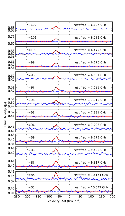
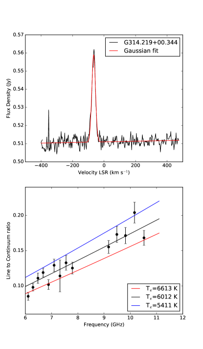
Figure 2: Spectra from a bright but previously unknown source. This figure shows the spectra for G314.219+00.344, which is a moderate to strong source, not previously detected in RRL emission. Individual RRL transitions are shown on the left panel, the overall average with Gaussian fit is shown on the upper right. The lower-right panel shows the line-to-continuum ratio for each RRL transition vs. frequency. Fitting these data with the assumption that both the line and continuum emission are optically thin gives an electron temperature T${}_{e}\ \simeq$ 6000 K (black line). The red and blue lines correspond to increase and decrease by 10% of the best fit T_e, as indicated.

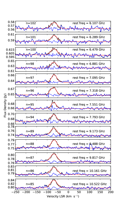
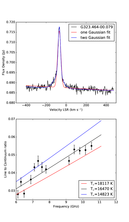
Figure 3: Spectra for a bright source that shows multiple linewidths. This figure shows the spectra for G323.464$-$00.079, which is a strong source, previously detected by Murphy et al. (2010), with panel layout the same as in Figure 2. This hypercompact H II region has a broad line profile that is not adequately fitted by a single Gaussian. This may indicate that there are two ionized regions with very different kinetic temperatures in the same H II region complex. The results of the two-Gaussian fit are given on Table 3, and indicated by “S2” in column 2.

A Gaussian fit was made to the line profile in the average spectrum for each candidate. For lines with SNR$>$3, the Gaussian parameters are given on Table 3, and illustrated on Figures 2 and 3. Table 3 gives for each detected source, the source name in column 1). Column 2 has an S (for “Source Average”) if the detection was made in the average of all RRL transitions or the Hn$\alpha$ number for sources bright enough to be detected in individual transitions. The following columns give the line center velocity (VLSR), line width (FWHM), continuum flux density ($S_{C}$), spectral rms noise, peak line flux density ($S_{L}$), electron temperature estimated from the line-to-continuum ratios ($T_{e}$), and the signal-to-noise ratio, SNR. The SNR is computed as (e.g. Lenz & Ayers, 1992):

$$SNR\ =\ 0.7\ \left(\frac{S_{L}}{RMS}\right)\ \sqrt{\frac{FWHM}{\Delta V}}$$ (1)

If a line was detected with signal-to-noise ratio greater than $\sim$15 in the average spectrum, then each individual Hn$\alpha$ transition was considered separately, again weighting the different baselines by their continuum flux. Gaussians were fitted to the average line profile for each transition. The results are listed as separate entries under each source name in Table 3. For these lines, the SNR is simply the peak line flux divided by its error.

For lines sufficiently strong that their peak can be determined fairly accurately for each transition separately, it is possible to estimate the electron temperature, under the assumption that both the spectral line and continuum emission are optically thin. Whether or not this assumption holds depends on the emission measure. Typically for diffuse H II regions the continuum is optically thin for frequencies above three to five GHz, but for ultracompact and hypercompact H II regions the continuum can be optically thick up to frequencies much higher than the C/X band observed here (4 to 11 GHz). If the line and continuum are both optically thin, and the level populations are in thermodynamic equilibrium with the electron kinetic temperature, $T_{e}$, then the line-to-continuum ratio, $S_{L}$ / $S_{C}$, is :

$$\frac{S_{L}}{S_{C}}\ =\ 7\times 10^{3}\ \left(\frac{\Delta V_{FWHM}}{\mathrm{km\ s}^{-1}}\right)^{-1}\ \left(\frac{\nu}{\mathrm{GHz}}\right)^{1.1}\ \left(\frac{T_{e}}{{\mathrm{K}}}\right)^{-1.15}\ \left(1\ +\ \frac{N(He^{+})}{N(H^{+})}\right)^{-1}$$ (2)

where $\Delta V_{FWHM}$ is the line width (full width to half maximum, or 2.35 times $\sigma_{v}$), $\nu$ is the line rest frequency, and the ratio of column densities of He⁺ to H⁺ is taken as 0.09, making the final term 1.09 (Quireza et al., 2006).

An interferometer telescope is particularly well suited to measurement of $T_{e}$, because each baseline at each frequency measures $S_{L}$ and $S_{C}$ through the same spatial filter or fringe pattern. Although different baselines measure different continuum flux values, depending on the angular size and structure of the source and the projected baseline length, there is no need to determine a zero-level or overall offset to the continuum flux, as there is for single-dish surveys. In principal, every Hn$\alpha$ transition provides a separate measurement of $T_{e}$ by equation 2 (column 8 on table 3). A better estimate is given by fitting the line-to-continuum ratios for all lines to a single $T_{e}$ value. This is shown for the two sample sources on the lower right panels of Figures 2 and 3.

The second example, G323.464$-$00.079, is a hyper-compact H II region that violates the condition of being optically thin in the continuum (Murphy et al., 2010). Unlike most of our detections, including G314.219+00.344 shown on Figure 2, the continuum flux of G323.464$-$00.079 increases rapidly with increasing frequency across the entire range of these observations. In this case the electron temperature derived from the line-to-continuum ratios is an overestimate. Further study of this source using maps of the RRL emission may reveal whether the two Gaussian components correspond to separate regions of ionized gas.

Accurate values of the continuum and spectral line flux densities will require mapping and cleaning of the interferometer data. The full SHRDS survey achieves much better coverage of the uv plane, as it uses two different array configurations and longer integrations at more and different hour angles. Thus the values on columns 5 and 7 of Table 3 will be revised when better data become available. But the line to continuum ratios, and hence the electron temperatures, can be determined quickly from the uv data alone, as shown in the lower right panels of Figures 2 and 3.

5 Summary and Conclusions

The SHRDS Pilot Study discovered 36 H II regions with radio recombination lines, a detection rate of about 66%. All known H II regions included in the observing schedule were also successfully re-detected. More than one third (15 out of 35) of the newly discovered H II regions are located in the outer Galaxy where existing catalogs of H II regions are not very complete. For the sources with RRL detections in the literature, the line strengths, center velocities, and line widths are in good agreement with published values. The rms of the differences in centre velocities divided by their errors is 1.1, and the rms of the differences in FWHM divided by their errors is 1.4. The only velocity parameter that differs from its corresponding value in the literature by more than two sigma is the FWHM of the line in G295.748$-$00.207, which we find as 23.9$\pm$3.5 km s^-1 vs. Caswell & Haynes (1987) value of 35 km s^-1. Caswell & Haynes (1987) do not give an error in the FWHM, but their channel spacing is 2.3 km s^-1.

A surprising result of these pilot observations is the low detection rate for candidate H II regions in the third quadrant compared with those in the fourth quadrant of the Galaxy. This may be caused in part by a selection bias against sources with large angular sizes. The interferometer is not sensitive to brightness that is smoothly spread over angular sizes larger than about 6′, as noted in section 3, paragraph 1. Thus nearby regions with large radii will show lower flux densities for the interferometer than they would to a single dish telescope.

The main goal of these pilot experiments was to demonstrate the efficiency and sensitivity of the ATCA for detecting RRL emission from Galactic H II regions using the CABB system. The secondary objective was to determine the best placement for the CABB zoom bands, given the varying system temperature and interference environment of the ATCA, and the typical emission spectra of a sample of H II region candidates. The result of the two epochs of observations indicates that the SHRDS should concentrate on the higher frequencies available with the 4 cm (C/X-band) receiver. These are generally easier to calibrate, more sensitive to RRLs from typical H II region candidates, and the resolution is better at shorter wavelengths.

The observing strategy for the SHRDS was also a subject of experimentation in the pilot project. For candidates near the detection threshold, an efficient strategy is to make many short observations, at widely spaced hour angles so as to get the best coverage of the $uv$ plane. These three or four minute integrations are not long enough to detect RRLs, but with five to ten such “snapshots” a continuum map with fair to good dynamic range can be made. Based on the strength of the source(s) found on the continuum map, we can estimate accurately the expected RRL line strength. The total telescope time available can then be apportioned among the candidates so as to optimise the line detection rate.

Table 3: Detected RRL Gaussian Parameters

Source	Hn$\alpha$	VLSR	FWHM	Sc	RMS	SL	Te	SNR
Name	(n)	(km s-1)	(km s-1)	(mJy)	(mJy)	(mJy)	(K)	$\sigma$
G$213.833+00.618$	S	$53.2\pm 20.2$	33.5 $\pm$ 20.9	N/A	1.4	1.9 $\pm$ 2.3	N/A	3.5
G$230.354-00.597$	S	$69.0\pm 16.1$	35.0 $\pm$ 16.7	N/A	1.5	2.1 $\pm$ 2.0	N/A	3.7
G$290.012-00.867$	S	$14.7\pm 8.3$	24.9 $\pm$ 8.6	N/A	1.8	3.6 $\pm$ 2.5	N/A	4.5
G$290.323-02.984$	S	$-17.7\pm 8.0$	28.3 $\pm$ 8.3	N/A	1.5	3.5 $\pm$ 2.1	N/A	5.6
G$290.385-01.042$	S	$9.91\pm 4.6$	13.2 $\pm$ 4.7	N/A	1.9	4.0 $\pm$ 2.9	N/A	3.4
G$290.674-00.133$	S	$19.3\pm 5.2$	23.2 $\pm$ 5.3	N/A	1.4	5.2 $\pm$ 2.4	N/A	8.0
G$291.596-00.239$	S	$11.4\pm 5.1$	44.2 $\pm$ 5.4	N/A	2.5	15.3 $\pm$ 3.7	8300 $\pm$ 1200	18.
G$292.889-00.831$	S	$21.8\pm 7.1$	30.0 $\pm$ 7.3	N/A	1.4	4.8 $\pm$ 2.3	N/A	8.4
G$293.936-00.873$	S	$36.6\pm 1.4$	22.3 $\pm$ 1.5	N/A	2.0	16.4 $\pm$ 2.2	9400 $\pm$ 400	17
G$293.994-00.934$	S	$46.5\pm 1.7$	25.6 $\pm$ 1.8	N/A	1.3	18.6 $\pm$ 2.6	9600 $\pm$ 400	32
G$294.988-00.538$	S	$39.8\pm 1.9$	27.4 $\pm$ 2.0	N/A	1.2	9.7 $\pm$ 1.4	10000 $\pm$ 400	19
G$295.275-00.255$	S	$30.1\pm 6.2$	30.6 $\pm$ 6.3	N/A	1.6	5.6 $\pm$ 2.3	7900 $\pm$ 4500	8.7
G$295.748-00.207$	S	$23.3\pm 3.5$	23.9 $\pm$ 3.5	N/A	1.6	7.2 $\pm$ 2.1	7300 $\pm$ 1800	9.8
G$297.248-00.754$	S	$22.6\pm 1.5$	24.4 $\pm$ 1.6	N/A	1.9	22.6 $\pm$ 2.9	7200 $\pm$ 400	26
	107	$24.4\pm 2.7$	23.1 $\pm$ 2.8	369	7.2	22.0 $\pm$ 5.0	7700 $\pm$ 3200	3.1
	106	$22.0\pm 2.8$	27.6 $\pm$ 2.8	365	7.0	21.0 $\pm$ 4.0	6900 $\pm$ 2300	3.0
	105	$22.3\pm 2.6$	25.8 $\pm$ 2.7	359	6.9	20.0 $\pm$ 4.0	7700 $\pm$ 2700	3.0
	104	$20.4\pm 2.3$	26.0 $\pm$ 2.3	356	8.3	25.0 $\pm$ 4.0	6500 $\pm$ 1900	3.1
	103	$22.3\pm 2.8$	25.3 $\pm$ 2.9	350	7.0	21.0 $\pm$ 4.0	7700 $\pm$ 3000	3.1
G$297.626-00.906$	S	$31.3\pm 2.1$	28.4 $\pm$ 2.2	N/A	1.5	16.1 $\pm$ 2.5	7900 $\pm$ 400	26
G$298.473+00.104$	S	$32.9\pm 2.0$	23.5 $\pm$ 2.1	N/A	2.0	12.2 $\pm$ 2.2	7900 $\pm$ 400	13
G$298.669+00.064$	S	$24.1\pm 2.4$	14.1 $\pm$ 2.4	N/A	2.2	11.4 $\pm$ 3.9	11000 $\pm$ 3800	8.7
G$300.972+00.994$	S	$-34.5\pm 7.2$	39.1 $\pm$ 7.5	N/A	1.7	3.8 $\pm$ 1.4	5600 $\pm$ 2600	6.3
G$300.983+01.117$	S	$-42.0\pm 0.4$	26.5 $\pm$ 0.4	N/A	3.3	83.8 $\pm$ 2.8	6000 $\pm$ 880	26.0
	107	$-42.4\pm 0.8$	25.6 $\pm$ 0.9	1360	12.3	86.0 $\pm$ 5.0	6700 $\pm$ 650	7.0
	106	$-43.0\pm 0.9$	25.2 $\pm$ 0.9	1330	12.6	86.0 $\pm$ 6.0	6800 $\pm$ 690	6.8
	105	$-42.7\pm 0.8$	27.2 $\pm$ 0.8	1290	13.2	91.0 $\pm$ 5.0	6100 $\pm$ 530	6.9
	104	$-41.9\pm 1.0$	26.2 $\pm$ 1.0	1260	13.3	83.0 $\pm$ 6.0	6900 $\pm$ 780	6.3
	103	$-42.0\pm 1.0$	25.7 $\pm$ 1.0	1220	12.6	85.0 $\pm$ 6.0	6800 $\pm$ 770	6.8
	96	$-42.2\pm 1.0$	26.0 $\pm$ 1.0	879	22.5	81.0 $\pm$ 6.0	6500 $\pm$ 720	3.6
	94	$-41.2\pm 1.0$	24.9 $\pm$ 1.0	809	20.0	75.0 $\pm$ 6.0	7100 $\pm$ 850	3.8
	93	$-40.6\pm 1.1$	26.6 $\pm$ 1.1	750	17.7	73.0 $\pm$ 6.0	6600 $\pm$ 810	4.2
G$313.671-00.104$	S	$-54.6\pm 1.4$	24.6 $\pm$ 1.5	N/A	1.6	12.0 $\pm$ 1.4	6700 $\pm$ 400	17
G$313.790+00.706$	S	$-57.2\pm 0.9$	22.6 $\pm$ 0.9	N/A	2.6	38.7 $\pm$ 3.0	7000 $\pm$ 450	32
	101	$-57.6\pm 1.9$	20.2 $\pm$ 1.9	436	11.1	41.0 $\pm$ 8.0	6800 $\pm$ 2200	3.7
	97	$-56.7\pm 1.8$	20.6 $\pm$ 1.8	399	11.2	38.0 $\pm$ 6.0	7300 $\pm$ 2100	3.5
	96	$-56.8\pm 2.6$	26.9 $\pm$ 2.6	396	11.8	35.0 $\pm$ 6.0	6400 $\pm$ 2100	3.0
	95	$-55.0\pm 2.2$	26.4 $\pm$ 2.3	386	11.7	35.0 $\pm$ 6.0	6600 $\pm$ 1800	3.1
	94	$-58.5\pm 1.6$	20.7 $\pm$ 1.6	372	12.8	41.0 $\pm$ 6.0	7100 $\pm$ 1700	3.2
	89	$-55.7\pm 1.7$	21.7 $\pm$ 1.8	330	11.9	39.0 $\pm$ 6.0	7400 $\pm$ 1900	3.3
	87	$-57.0\pm 1.8$	21.3 $\pm$ 1.9	306	11.9	40.0 $\pm$ 7.0	7500 $\pm$ 2200	3.4
	85	$-56.2\pm 1.7$	22.2 $\pm$ 1.8	294	13.8	42.0 $\pm$ 6.0	7100 $\pm$ 1800	3.1
G$314.219+00.344$	S	$-62.5\pm 0.4$	20.0 $\pm$ 0.5	N/A	3.5	66.4 $\pm$ 3.1	6500 $\pm$ 640	38
	101	$-63.0\pm 1.0$	21.0 $\pm$ 1.0	706	12.8	81.0 $\pm$ 7.0	5600 $\pm$ 780	6.3
	97	$-62.7\pm 0.9$	18.1 $\pm$ 0.9	534	12.3	71.0 $\pm$ 7.0	6200 $\pm$ 940	5.8
	96	$-61.7\pm 1.4$	20.6 $\pm$ 1.4	495	12.2	55.0 $\pm$ 7.0	6700 $\pm$ 1400	4.6
	95	$-63.1\pm 1.2$	18.4 $\pm$ 1.2	468	12.1	63.0 $\pm$ 8.0	6500 $\pm$ 1300	5.2
	94	$-62.1\pm 1.2$	21.8 $\pm$ 1.2	438	12.9	59.0 $\pm$ 6.0	5700 $\pm$ 990	4.6
	89	$-61.6\pm 1.2$	21.2 $\pm$ 1.2	401	12.5	57.0 $\pm$ 6.0	6500 $\pm$ 1100	4.6
	87	$-62.7\pm 1.0$	18.6 $\pm$ 1.0	389	13.0	67.0 $\pm$ 7.0	6700 $\pm$ 1100	5.1
	85	$-62.5\pm 1.5$	20.1 $\pm$ 1.6	360	15.3	65.0 $\pm$ 10.0	6400 $\pm$ 1600	4.3
G$315.312-00.273$	S	$14.2\pm 1.4$	24.0 $\pm$ 1.4	N/A	3.6	30.0 $\pm$ 3.6	7700 $\pm$ 400	18
	101	$10.7\pm 2.1$	18.1 $\pm$ 2.2	414	11.5	37.0 $\pm$ 9.0	7800 $\pm$ 3300	3.3
	97	$14.1\pm 2.4$	22.4 $\pm$ 2.4	377	11.9	36.0 $\pm$ 7.0	6900 $\pm$ 2500	3.1
	85	$15.2\pm 4.5$	33.4 $\pm$ 4.7	240	14.9	22.0 $\pm$ 6.0	7400 $\pm$ 3900	1.5
G$316.516-00.600$	S	$-45.6\pm 0.9$	19.9 $\pm$ 0.9	N/A	1.7	19.0 $\pm$ 1.7	5900 $\pm$ 400	22
	97	$-46.2\pm 2.0$	18.1 $\pm$ 2.0	142	6.1	20.0 $\pm$ 4.0	5900 $\pm$ 2300	3.3
	96	$-45.4\pm 2.0$	19.4 $\pm$ 2.0	140	6.5	20.0 $\pm$ 4.0	5500 $\pm$ 2000	3.2
	94	$-46.2\pm 1.8$	18.2 $\pm$ 1.9	135	6.6	21.0 $\pm$ 4.0	5900 $\pm$ 2100	3.2
	89	$-42.7\pm 1.8$	19.8 $\pm$ 1.8	115	6.7	21.0 $\pm$ 3.0	5600 $\pm$ 1700	3.2
	87	$-45.8\pm 1.9$	20.3 $\pm$ 1.9	106	6.9	21.0 $\pm$ 4.0	5300 $\pm$ 1700	3.2
G$317.861+00.160$	S	$1.53\pm 0.9$	22.9 $\pm$ 0.9	N/A	2.7	55.6 $\pm$ 4.6	7600 $\pm$ 430	44
	101	$1.68\pm 1.7$	24.4 $\pm$ 1.7	713	13.0	55.0 $\pm$ 7.0	6900 $\pm$ 1500	4.2
	97	$2.22\pm 1.6$	25.0 $\pm$ 1.6	648	13.2	55.0 $\pm$ 7.0	7000 $\pm$ 1400	4.2
	96	$1.49\pm 1.3$	19.6 $\pm$ 1.4	631	13.8	66.0 $\pm$ 9.0	7400 $\pm$ 1600	4.8
	95	$1.24\pm 1.5$	20.7 $\pm$ 1.5	614	13.3	54.0 $\pm$ 8.0	8400 $\pm$ 2000	4.1
	94	$2.88\pm 1.9$	28.5 $\pm$ 2.0	597	14.4	53.0 $\pm$ 7.0	6600 $\pm$ 1400	3.7
	89	$0.942\pm 1.4$	21.3 $\pm$ 1.5	506	13.9	55.0 $\pm$ 7.0	8200 $\pm$ 1700	4.0
	87	$0.801\pm 1.7$	23.8 $\pm$ 1.8	466	14.8	52.0 $\pm$ 7.0	7800 $\pm$ 1800	3.5
	85	$-0.447\pm 2.4$	29.8 $\pm$ 2.5	431	16.5	49.0 $\pm$ 8.0	6800 $\pm$ 1900	3.0
G$318.248+00.151$	S	$-39.9\pm 2.0$	19.0 $\pm$ 2.0	N/A	2.8	17.0 $\pm$ 3.7	5900 $\pm$ 740	12
	101	$-43.0\pm 1.7$	12.2 $\pm$ 1.7	175	11.0	34.0 $\pm$ 10.0	5500 $\pm$ 3000	3.2
G$319.229+00.225$	S	$-66.1\pm 1.8$	20.9 $\pm$ 1.8	N/A	1.9	12.9 $\pm$ 2.2	6800 $\pm$ 400	14
G$323.449+00.095$	S	$-75.1\pm 1.7$	22.5 $\pm$ 1.7	N/A	2.0	13.8 $\pm$ 2.1	5900 $\pm$ 400	15
G$323.464-00.079$	S	$-68.8\pm 1.2$	38.3 $\pm$ 1.2	N/A	1.3	28.0 $\pm$ 2.2	11000 $\pm$ 1700	45
	S2	$-68.1\pm 1.2$	27.7 $\pm$ 2	N/A	1.3	24 $\pm$ 2.2		21
	S2	$-77.2\pm 1.2$	105.5 $\pm$ 10	N/A	1.3	6.5 $\pm$ 2.2		4.9
	101	$-66.4\pm 2.5$	31.2 $\pm$ 2.6	589	6.3	20.0 $\pm$ 3.0	11000 $\pm$ 2900	3.2
	97	$-67.1\pm 1.7$	27.7 $\pm$ 1.8	636	6.2	26.0 $\pm$ 3.0	12000 $\pm$ 2300	4.3
	96	$-67.1\pm 1.8$	27.3 $\pm$ 1.9	649	6.6	26.0 $\pm$ 3.0	13000 $\pm$ 2700	4.0
	95	$-67.7\pm 2.0$	27.3 $\pm$ 2.1	661	6.5	24.0 $\pm$ 3.0	14000 $\pm$ 3400	3.8
	94	$-69.3\pm 1.9$	30.7 $\pm$ 1.9	673	7.1	27.0 $\pm$ 3.0	12000 $\pm$ 2200	3.9
	89	$-68.5\pm 1.6$	35.2 $\pm$ 1.6	746	7.7	35.0 $\pm$ 3.0	11000 $\pm$ 1500	4.6
	87	$-68.6\pm 1.3$	36.6 $\pm$ 1.3	770	8.2	40.0 $\pm$ 2.0	11000 $\pm$ 1100	4.9
	85	$-68.8\pm 1.4$	36.9 $\pm$ 1.4	804	9.2	42.0 $\pm$ 3.0	11000 $\pm$ 1200	4.7
G$323.743-00.249$	S	$-47.3\pm 0.7$	19.2 $\pm$ 0.7	N/A	2.2	22.8 $\pm$ 1.8	6000 $\pm$ 400	20
	101	$-47.3\pm 1.9$	17.0 $\pm$ 1.9	165	6.9	22.0 $\pm$ 5.0	5800 $\pm$ 2300	3.2
	97	$-46.7\pm 1.6$	17.7 $\pm$ 1.6	160	6.8	25.0 $\pm$ 4.0	5500 $\pm$ 1700	3.8
	95	$-47.7\pm 2.0$	19.2 $\pm$ 2.1	157	6.8	21.0 $\pm$ 4.0	6100 $\pm$ 2300	3.2
	89	$-47.8\pm 1.4$	17.3 $\pm$ 1.4	147	7.1	27.0 $\pm$ 4.0	6300 $\pm$ 1600	3.8
	87	$-47.6\pm 1.6$	21.7 $\pm$ 1.7	141	7.3	26.0 $\pm$ 4.0	5400 $\pm$ 1400	3.6
	85	$-46.1\pm 2.3$	19.4 $\pm$ 2.4	138	7.6	25.0 $\pm$ 6.0	6600 $\pm$ 3000	3.3
G$323.806+00.021$	S	$-58.9\pm 0.9$	21.6 $\pm$ 0.9	N/A	2.7	31.6 $\pm$ 2.7	7200 $\pm$ 400	24
	101	$-57.4\pm 2.0$	18.8 $\pm$ 2.0	373	10.0	35.0 $\pm$ 7.0	7300 $\pm$ 2700	3.5
	97	$-57.0\pm 1.7$	18.4 $\pm$ 1.7	333	10.0	36.0 $\pm$ 6.0	7400 $\pm$ 2300	3.6
	96	$-59.3\pm 2.1$	25.4 $\pm$ 2.1	320	10.4	37.0 $\pm$ 6.0	5400 $\pm$ 1400	3.6
	89	$-59.4\pm 1.8$	21.0 $\pm$ 1.9	248	11.0	35.0 $\pm$ 6.0	6700 $\pm$ 2000	3.2
G$323.936-00.037$	S	$-57.3\pm 4.5$	24.5 $\pm$ 4.6	N/A	2.4	13.8 $\pm$ 5.2	5600 $\pm$ 2600	12.7
G$324.662-00.331$	S	$-47.8\pm 1.7$	21.3 $\pm$ 1.8	N/A	2.9	28.7 $\pm$ 4.8	7200 $\pm$ 400	20
G$325.108+00.054$	S	$-67.8\pm 2.7$	20.4 $\pm$ 2.7	N/A	3.2	11.5 $\pm$ 3.1	6700 $\pm$ 1600	7.3
G$325.354-00.035$	S	$-63.8\pm 0.6$	$34.4\pm 1.5$	N/A	1.4	$15\pm 1.5$	$6800\pm 800$	26
	102	-63.3 $\pm$ 1.4	25.2 $\pm$ 3.4	251	4.4	17 $\pm$ 2.0	7232 $\pm$ 970	8.7
	101	-68.8 $\pm$ 2.0	31.3 $\pm$ 4.7	252	4.6	14 $\pm$ 1.9	7168 $\pm$ 1100	7.7
	100	-62.7 $\pm$ 2.0	36.8 $\pm$ 4.8	246	5.2	17 $\pm$ 2.0	5335 $\pm$ 690	8.9
	98	-59.1 $\pm$ 1.1	19.6 $\pm$ 2.7	235	6.1	26 $\pm$ 3.1	6630 $\pm$ 920	8.4
	97	-61.4 $\pm$ 2.4	37.9 $\pm$ 6.0	228	5.5	19 $\pm$ 2.1	4934 $\pm$ 800	9.2
	96	-60.2 $\pm$ 1.3	19.4 $\pm$ 3.4	222	6.0	24 $\pm$ 3.2	7142 $\pm$ 1300	7.7
	95	-62.5 $\pm$ 2.0	27.4 $\pm$ 4.7	217	5.6	16 $\pm$ 2.4	7574 $\pm$ 1400	6.7
	94	-65.4 $\pm$ 1.8	32.2 $\pm$ 4.3	211	5.0	17 $\pm$ 2.0	6244 $\pm$ 830	8.7
	89	-63.8 $\pm$ 2.1	31.3 $\pm$ 5.1	183	4.6	13 $\pm$ 1.8	8501 $\pm$ 1400	7.1
	88	-60.6 $\pm$ 1.6	28.9 $\pm$ 3.7	178	4.6	17 $\pm$ 1.9	7130 $\pm$ 910	9.0
	87	-60.9 $\pm$ 1.3	30.1 $\pm$ 3.1	172	4.6	22 $\pm$ 1.9	5746 $\pm$ 570	11.4
	86	-56.5 $\pm$ 1.8	25.9 $\pm$ 4.3	167	5.7	18 $\pm$ 2.5	7869 $\pm$ 1350	7.0
	85	-59.8 $\pm$ 1.3	21.7 $\pm$ 3.1	162	5.2	21 $\pm$ 2.5	8035 $\pm$ 1140	8.2
G$326.721+00.773$	S	$-40.6\pm 0.9$	22.6 $\pm$ 0.9	N/A	4.9	45.5 $\pm$ 3.7	6300 $\pm$ 400	20
	101	$-40.9\pm 2.0$	18.8 $\pm$ 2.0	458	14.3	51.0 $\pm$ 11.0	6300 $\pm$ 2300	3.6
	97	$-40.6\pm 2.0$	23.8 $\pm$ 2.0	470	15.4	53.0 $\pm$ 9.0	5700 $\pm$ 1500	3.5
	96	$-40.2\pm 2.0$	25.4 $\pm$ 2.1	480	16.4	56.0 $\pm$ 9.0	5400 $\pm$ 1400	3.5
	95	$-40.3\pm 2.2$	22.0 $\pm$ 2.2	466	15.7	46.0 $\pm$ 9.0	7200 $\pm$ 2400	3.0
G$326.890-00.277$	S	$-44.2\pm 0.7$	19.1 $\pm$ 0.7	N/A	3.5	63.2 $\pm$ 4.5	6200 $\pm$ 440	35
	101	$-45.4\pm 1.8$	19.4 $\pm$ 1.8	487	13.0	49.0 $\pm$ 9.0	6700 $\pm$ 2000	3.8
	97	$-43.7\pm 1.2$	18.1 $\pm$ 1.2	465	13.4	65.0 $\pm$ 8.0	6000 $\pm$ 1200	4.9
	96	$-45.0\pm 1.8$	22.6 $\pm$ 1.9	456	13.8	53.0 $\pm$ 8.0	5900 $\pm$ 1600	3.9
	95	$-45.3\pm 1.6$	22.2 $\pm$ 1.7	450	13.6	54.0 $\pm$ 8.0	6000 $\pm$ 1400	4.0
	94	$-43.4\pm 1.2$	18.3 $\pm$ 1.2	445	15.7	62.0 $\pm$ 8.0	6500 $\pm$ 1300	4.0
	89	$-43.7\pm 0.9$	18.7 $\pm$ 0.9	415	13.9	75.0 $\pm$ 7.0	6000 $\pm$ 880	5.4
	87	$-44.3\pm 0.9$	20.5 $\pm$ 1.0	408	14.3	77.0 $\pm$ 7.0	5600 $\pm$ 800	5.5
	85	$-43.7\pm 0.8$	17.9 $\pm$ 0.8	396	15.1	80.0 $\pm$ 7.0	6400 $\pm$ 900	5.3
G$326.916-01.100$	S	$-49.8\pm 1.8$	21.0 $\pm$ 1.9	N/A	4.4	18.9 $\pm$ 3.4	6800 $\pm$ 450	8.8
G$327.313-00.536$	S	$-48.5\pm 0.2$	28.1 $\pm$ 0.3	N/A	33.1	2280.0 $\pm$ 41.7	6100 $\pm$ 890	163
	102	$-48.8\pm 0.4$	28.8 $\pm$ 0.4	26600	200.0	2020.0 $\pm$ 56.0	5900 $\pm$ 400	10.0
	101	$-48.9\pm 0.3$	28.5 $\pm$ 0.3	27000	211.0	2128.0 $\pm$ 47.0	5900 $\pm$ 400	10.0
	97	$-48.7\pm 0.3$	28.0 $\pm$ 0.3	25100	239.0	2226.0 $\pm$ 46.0	6100 $\pm$ 400	9.3
	96	$-48.7\pm 0.3$	28.0 $\pm$ 0.3	24600	238.0	2293.0 $\pm$ 48.0	6000 $\pm$ 400	9.6
	95	$-48.6\pm 0.3$	28.2 $\pm$ 0.3	24100	234.0	2289.0 $\pm$ 50.0	6100 $\pm$ 400	9.8
	94	$-48.5\pm 0.3$	27.6 $\pm$ 0.3	23500	303.0	2315.0 $\pm$ 53.0	6200 $\pm$ 400	7.6
	89	$-48.6\pm 0.3$	28.1 $\pm$ 0.3	20300	270.0	2420.0 $\pm$ 50.0	6000 $\pm$ 400	9.0
	87	$-48.3\pm 0.3$	27.6 $\pm$ 0.3	19100	282.0	2479.0 $\pm$ 53.0	6100 $\pm$ 400	8.8
	85	$-47.9\pm 0.3$	27.3 $\pm$ 0.3	18000	290.0	2471.0 $\pm$ 53.0	6200 $\pm$ 400	8.5
G$327.401+00.484$	S	$-76.3\pm 1.7$	17.7 $\pm$ 1.7	N/A	2.6	31.5 $\pm$ 6.1	6000 $\pm$ 570	23
	97	$-77.1\pm 1.6$	17.0 $\pm$ 1.7	229	13.7	47.0 $\pm$ 9.0	4500 $\pm$ 1500	3.5
G$327.555-00.829$	S	$-41.7\pm 2.6$	24.8 $\pm$ 2.6	N/A	4.0	16.5 $\pm$ 3.5	7500 $\pm$ 950	9.2
G$327.714+00.577$	S	$-47.4\pm 2.4$	21.9 $\pm$ 2.5	N/A	2.1	12.0 $\pm$ 2.7	6600 $\pm$ 1000	12
G$327.763+00.163$	S	$-92.8\pm 1.2$	21.6 $\pm$ 1.2	N/A	2.6	30.1 $\pm$ 3.4	6800 $\pm$ 400	24
	97	$-93.5\pm 2.1$	19.8 $\pm$ 2.1	297	10.3	33.0 $\pm$ 7.0	6700 $\pm$ 2500	3.3
	94	$-93.5\pm 1.8$	21.2 $\pm$ 1.8	265	10.7	37.0 $\pm$ 6.0	5700 $\pm$ 1600	3.5
	87	$-92.9\pm 2.0$	19.2 $\pm$ 2.0	191	10.8	35.0 $\pm$ 7.0	6100 $\pm$ 2300	3.3

References

- Anderson et al. (2015) Anderson, L. D., Armentrout, W.P., Johnstone, B.M., Bania, T. M., Balser, D. S., et al. 2015, ApJS, 221, 26
- Anderson et al. (2014) Anderson, L. D., Bania, T. M., Balser, D. S., et al. 2014, ApJS, 212, 1
- Anderson et al. (2011) Anderson, L. D., Bania, T. M., Balser, D. S., & Rood, R. T. 2011, ApJS, 194, 32
- Balser (2006) Balser, D. S. 2006, AJ, 132, 2326
- Bania et al. (2010) Bania, T. M., Anderson, L. D., Balser, D. S., & Rood, R. T. 2010, ApJ, 718, L106
- Bania et al. (2012) Bania, T. M., Anderson, L. D., & Balser, D. S. 2012, ApJ, 759, 96
- Benjamin et al. (2003) Benjamin, R.A., Churchwell, E., Babler, B.L., Bania, T.M., Clemens, D.P. et al. 2003, PASP 115, 953.
- Bock et al. (1999) Bock, D. C.-J., Large, M. I., & Sadler, E. M. 1999, AJ, 117, 1578
- Carey et al. (2009) Carey, S.J., Noriega-Crespo, A., Mizuno, D.R., Shenoy, S., Paladini, R., et al. 2009, PASP 121, 76.
- Caswell & Haynes (1987) Caswell, J. L., & Haynes, R. F. 1987, A&A, 171, 261
- Churchwell et al. (2009) Churchwell, E., Babler, B. L., Meade, M. R., et al. 2009, PASP, 121, 213
- Condon et al. (1998) Condon, J. J., Cotton, W. D., Greisen, E. W., et al. 1998, AJ, 115, 1693
- Helfand et al. (2006) Helfand, D. J., Becker, R. H., White, R. L., Fallon, A., & Tuttle, S. 2006, AJ, 131, 2525
- Hoare et al. (2012) Hoare, M.G., Purcell, C.R., Churchwell, E.B., Diamond, P., Cotton, W.D., et al. 2012, PASP124, 939.
- Hunter (2007) Hunter, J. D. 2007, Computing In Science & Engineering, 9, 90
- Lenz & Ayers (1992) Lenz, D.D. and Ayres, T.R., 1992, PASP, 104, 1104
- McClure-Griffiths et al. (2005) McClure-Griffiths, N. M., Dickey, J. M., Gaensler, B. M., et al. 2005, ApJS, 158, 178
- Misanovic et al. (2002) Misanovic, Z., Cram, L., & Green, A. 2002, MNRAS, 335, 114
- Murphy et al. (2010) Murphy, T., Cohen, M., Ekers, R. D., et al. 2010, MNRAS, 405, 1560
- Purcell et al. (2012) Purcell, C. R., Longmore, S. N., Walsh, A. J., et al. 2012, MNRAS, 426, 1972
- Purcell et al. (2013) Purcell, C. R., Hoare, M. G., Cotton, W. D., Lumsden, S. L., Urquhart, J. S., et al. 2013, Ap. J. Supp. 205, 1.
- Quireza et al. (2006) Quireza, C., Rood, R. T., Bania, T. M., Balser, D. S., & Maciel, W. J. 2006, ApJ, 653, 1226
- Sault et al. (1995) Sault, R. J., Teuben, P. J., & Wright, M. C. H. 1995, Astronomical Data Analysis Software and Systems IV, 77, 433
- Shaver et al. (1983) Shaver, P. A., McGee, R. X., Newton, L. M., Danks, A. C., & Pottasch, S. R. 1983, MNRAS, 204, 53
- Umana et al. (2015) Umana, G., Trigilio, C., Franzen, T. M. O., Norris, R. P., Leto, P. et al., 2015, MNRAS, 454, 902.
- Wilson et al. (2011) Wilson, W. E., Ferris, R. H., Axtens, P., et al. 2011, MNRAS, 416, 832
- Wright et al. (2010) Wright, E. L., Eisenhardt, P. R. M., Mainzer, A. K., et al. 2010, AJ, 140, 1868