Discontinuous Hamiltonian Monte Carlo
for discrete parameters and discontinuous likelihoods

Abstract

Hamiltonian Monte Carlo has emerged as a standard tool for posterior computation. In this article, we present an extension that can efficiently explore target distributions with discontinuous densities. Our extension in particular enables efficient sampling from ordinal parameters though embedding of probability mass functions into continuous spaces. We motivate our approach through a theory of discontinuous Hamiltonian dynamics and develop a corresponding numerical solver. The proposed solver is the first of its kind, with a remarkable ability to exactly preserve the Hamiltonian. We apply our algorithm to challenging posterior inference problems to demonstrate its wide applicability and competitive performance.

1 Introduction

Markov chain Monte Carlo is routinely used to generate samples from posterior distributions. While specialized algorithms exist for restricted model classes, general-purpose algorithms are often inefficient and scale poorly in the number of parameters. Originally proposed by Duane et al. (1987) and popularized in the statistics community through the works of Neal (1996, 2010), Hamiltonian Monte Carlo promises a better scalability (Neal, 2010; Beskos et al., 2013) and has enjoyed wide-ranging successes as one of the most reliable approaches in general settings (Gelman et al., 2013; Kruschke, 2014; Monnahan et al., 2017).

However, a fundamental limitation of Hamiltonian Monte Carlo is the lack of support for discrete parameters (Gelman et al., 2015; Monnahan et al., 2017). The difficulty stems from the fact that the construction of Hamiltonian Monte Carlo proposals relies on a numerical solution of a differential equation. The use of a surrogate differentiable target distribution may be possible in special cases (Zhang et al., 2012), but approximating a discrete parameter of a likelihood by a continuous one is difficult in general (Berger et al., 2012).

This article presents discontinuous Hamiltonian Monte Carlo, an extension that can efficiently explore spaces involving ordinal discrete parameters as well as continuous ones. The algorithm can also handle discontinuities in piecewise smooth posterior densities, which for example arise from models with structural change points (Chib, 1998; Wagner et al., 2002), latent thresholds (Neelon & Dunson, 2004; Nakajima & West, 2013), and pseudo-likelihoods (Bissiri et al., 2016).

Discontinuous Hamiltonian Monte Carlo retains the generality that makes Hamiltonian Monte Carlo suitable for automatic posterior inference. For any given target distribution, each iteration only requires evaluations of the density and of the following quantities up to normalizing constants: 1) full conditional densities of discrete parameters, and 2) either the gradient of the log density with respect to continuous parameters or their individual full conditional densities. Evaluations of full conditionals can be done algorithmically and efficiently through directed acyclic graph frameworks, taking advantage of conditional independence structures (Lunn et al., 2009). Algorithmic evaluation of the gradient is also efficient (Griewank & Walther, 2008) and its implementations are widely available as open-source modules (Carpenter et al., 2015).

In our framework, the discrete parameters are first embedded into a continuous space, inducing parameters with piecewise constant densities. A key theoretical insight is that Hamiltonian dynamics with a discontinuous potential energy can be integrated analytically near its discontinuity in a way that exactly preserves the total energy. This fact was realized by Pakman & Paninski (2013) and used to sample from binary distributions through embedding them into a continuous space. This framework was extended by Afshar & Domke (2015) to handle more general discontinuous distributions and then by Dinh et al. (2017) to settings where the parameter space involves phylogenetic trees. All these frameworks, however, run into serious computational issues when dealing with more complex discontinuities and thus fail as general-purpose algorithms.

We introduce novel techniques to obtain a practical sampling algorithm for discrete parameters and, more generally, target distributions with discontinuous densities. In dealing with discontinuous targets, we propose a Laplace distribution for the momentum variable as a more effective alternative to the usual Gaussian distribution. We develop an efficient integrator of the resulting Hamiltonian dynamics by splitting the differential operator into its coordinate-wise components. A version of discontinuous Hamiltonian Monte Carlo coincides with a generalization of Metropolis-within-Gibbs samplers, overcoming dependency among the parameters by adding momentum along each coordinate.

2 Hamiltonian Monte Carlo for discrete and discontinuous distributions

2.1 Review of Hamiltonian Monte Carlo

Given a parameter $\bm{\theta}\sim\pi_{\Theta}(\cdot)$ of interest, Hamiltonian Monte Carlo introduces an auxiliary momentum variable $\bm{p}$ and samples from a joint distribution $\pi(\bm{\theta},\bm{p})=\pi_{\Theta}(\bm{\theta})\pi_{P}(\bm{p})$ for some symmetric distribution $\pi_{P}(\bm{p})\propto\exp\{-K(\bm{p})\}$. The function $K(\bm{p})$ is referred to as the kinetic energy and $U(\bm{\theta})=-\log\pi_{\Theta}(\bm{\theta})$ as the potential energy. The total energy $H(\bm{\theta},\bm{p})=U(\bm{\theta})+K(\bm{p})$ is often called the Hamiltonian. A proposal is generated by simulating trajectories of Hamiltonian dynamics where the evolution of the state $(\bm{\theta},\bm{p})$ is governed by Hamilton’s equations:

$$\frac{\textrm{d}\bm{\theta}}{\textrm{d}t} =\nabla_{\bm{p}}K(\bm{p}),\quad\frac{\textrm{d}\bm{p}}{\textrm{d}t}=-\nabla_{\bm{\theta}}U(\bm{\theta})=\nabla_{\bm{\theta}}\log\pi_{\Theta}(\bm{\theta}).$$ (1)

The next section shows how we can turn the problem of dealing with a discrete parameter $\bm{\theta}$ to that of dealing with a discontinuous target density. We then proceed to make sense of the differential equation (1) when $\pi_{\Theta}(\bm{\theta})$, and hence $U(\bm{\theta})$, is discontinuous.

2.2 Dealing with discrete parameters via embedding

Let $N$ denote a discrete parameter with the prior distribution $\pi_{N}(\cdot)$ and assume without loss of generality that $N$ takes positive integer values. For example, the inference goal may be estimation of the population size $N$ given the observation $y\,|\,q,N\sim\mathrm{Binomial}(q,N)$. We embed $N$ into a continuous space by introducing a latent parameter $\widetilde{N}$ whose relationship to $N$ is defined as

$$N=n\quad\text{ if and only if }\quad\widetilde{N}\in(a_{n},a_{n+1}],$$ (2)

for an increasing sequence of real numbers $0=a_{1}\leq a_{2}\leq a_{3}\leq\ldots$. To match the prior distribution on $N$, we define the corresponding prior density on $\widetilde{N}$ as

$$\pi_{\widetilde{N}}(\tilde{n})=\sum_{n\geq 1}\frac{\pi_{N}(n)}{a_{n+1}-a_{n}}\,\mathbbm{1}\{a_{n}<\tilde{n}\leq a_{n+1}\},$$ (3)

where the Jacobian-like factor $(a_{n+1}-a_{n})^{-1}$ adjusts for embedding into non-uniform intervals.

Although the choice $a_{n}=n$ for all $n$ is a natural one, a non-uniform embedding is useful in effectively carrying out a parameter transformation of $N$. For example, a log-transform $a_{n}=\log n$ may be used to avoid a heavy-tailed distribution on $\widetilde{N}$ or to reduce correlation between $\widetilde{N}$ and the rest of the parameters. Mixing of many Markov chain Monte Carlo algorithms, including discontinuous Hamiltonian Monte Carlo, can be substantially improved by such parameter transformations (Roberts & Rosenthal, 2009; Thawornwattana et al., 2018).

While the above strategy can be applied whether or not the discrete parameter values have a natural ordering, embedding the values in an arbitrary order likely induces a multi-modal continuous distribution. The mixing rate of (discontinuous) Hamiltonian Monte Carlo generally suffers from multi-modality due to the energy-conservation property of the dynamics (Neal, 2010).

2.3 How Hamiltonian Monte Carlo fails on discontinuous target densities

Having recast the discrete parameter problem as a discontinuous one, we focus the rest of our discussion on discontinuous targets. An integrator is an algorithm that numerically approximates an evolution of the exact solution to a differential equation. Hamiltonian Monte Carlo requires reversible and volume-preserving integrators to guarantee symmetry of its proposal distributions (see Section 4.1 and Neal, 2010). These proposals are generated as follows:

1. Sample the momentum from its marginal distribution $\bm{p}\sim\pi_{P}(\cdot)$.

2. Using a reversible and volume-preserving integrator, approximate $\{\bm{\theta}(t),\bm{p}(t)\}_{t\geq 0}$, the solution of the differential equation (1) with the initial condition $\{\bm{\theta}(0),\bm{p}(0)\}=(\bm{\theta},\bm{p})$. Use the approximate solution $(\bm{\theta}^{*},\bm{p}^{*})\approx\{\bm{\theta}(\tau),\bm{p}(\tau)\}$ for some $\tau>0$ as a proposal.

The proposal $(\bm{\theta}^{*},\bm{p}^{*})$ then is accepted with Metropolis probability (Metropolis et al., 1953)

$$\min\left[1,\ \exp\{-H(\bm{\theta}^{*},\bm{p}^{*})+H(\bm{\theta},\bm{p})\}\right],$$ (4)

where $H(\bm{\theta},\bm{p})=-\log\pi(\bm{\theta},\bm{p})$ denotes the Hamiltonian. With an accurate integrator, the acceptance probability of $(\bm{\theta}^{*},\bm{p}^{*})$ can be close to $1$ because the exact dynamics conserves the energy: $H\{\bm{\theta}(t),\bm{p}(t)\}=H\{\bm{\theta}(0),\bm{p}(0)\}$ for all $t\geq 0$. The integrator of choice for Hamiltonian Monte Carlo is the leapfrog scheme, which approximates the evolution $\{\bm{\theta}(t),\bm{p}(t)\}\to\{\bm{\theta}(t+\epsilon),\bm{p}(t+\epsilon)\}$ by the successive updates

$$\bm{p} \leftarrow\bm{p}-\frac{\epsilon}{2}\nabla_{\bm{\theta}}U(\bm{\theta}),\quad\bm{\theta}\leftarrow\bm{\theta}+\epsilon\nabla_{\bm{p}}K(\bm{p}),\quad\bm{p}\leftarrow\bm{p}-\frac{\epsilon}{2}\nabla_{\bm{\theta}}U(\bm{\theta}).$$ (5)

When $\pi_{\Theta}(\cdot)$ is smooth, approximating the evolution $\{\bm{\theta}(0),\bm{p}(0)\}\to\{\bm{\theta}(\tau),\bm{p}(\tau)\}$ with $L=\lfloor\tau/\epsilon\rfloor$ leapfrog steps results in a global error of order $O(\epsilon^{2})$ so that $H(\bm{\theta}^{*},\bm{p}^{*})=H(\bm{\theta},\bm{p})+O(\epsilon^{2})$ (Hairer et al., 2006). Hamiltonian Monte Carlo’s high acceptance rates and scaling properties critically depend on this second-order accuracy (Beskos et al., 2013). When $\pi_{\Theta}(\cdot)$ has a discontinuity, however, the leapfrog updates (5) fail to account for the instantaneous change in $\pi_{\Theta}(\cdot)$, incurring an unbounded error that does not decrease even as $\epsilon\to 0$ (supplement Section S1).

2.4 Theory of discontinuous Hamiltonian dynamics

Suppose $U(\theta)$ is piecewise smooth; that is, the domain has a partition $\mathbb{R}^{d}=\cup_{k}\Omega_{k}$ such that $U(\theta)$ is smooth on the interior of $\Omega_{k}$ and the boundary $\partial\Omega_{k}$ is a $(d-1)$-dimensional piecewise smooth manifold. While the classical definition of gradient $\nabla U(\bm{\theta})$ makes no sense on a discontinuity set $\cup_{k}\partial\Omega_{k}$, it can be defined through a notion of distributional derivatives and the corresponding Hamilton’s equations (1) can be interpreted as a measure-valued differential inclusion (Stewart, 2000). In this case, a solution is in general non-unique unlike that of a smooth ordinary differential equation. To find a solution that preserves critical properties of Hamiltonian dynamics, we rely on a so-called selection principle (Ambrosio, 2008) as follows.

Define a sequence of smooth approximations $U_{\delta}(\bm{\theta})$ of $U(\bm{\theta})$ for $\delta>0$ through the convolution $U_{\delta}(\theta):=\int U(\eta)\phi_{\delta}(\theta-\eta)\textrm{d}\eta$, where $\phi_{\delta}(\bm{\theta})=\delta^{-d}\phi(\delta^{-1}\bm{\theta})$ is a compactly supported smooth function with $\phi\geq 0$ and $\int\phi=1$. Now let $\{\bm{\theta}_{\delta}(t),\bm{p}_{\delta}(t)\}_{t\geq 0}$ be the solution of Hamilton’s equations with the potential energy $U_{\delta}$. The pointwise limit $\{\bm{\theta}(t),\bm{p}(t)\}=\lim_{\delta\to 0}\{\bm{\theta}_{\delta}(t),\bm{p}_{\delta}(t)\}$ can be shown to exist for almost every initial condition on some time interval $[0,T]$ (Hirsch & Smale, 1974). The collections of the trajectories $\left\{\{\bm{\theta}(t),\bm{p}(t)\}_{t\geq 0}:\{\bm{\theta}(0),\bm{p}(0)\}\in\mathbb{R}^{d}\right\}$ then define the dynamics corresponding to $U(\bm{\theta})$. This construction provides a rigorous mathematical foundation for the special cases of discontinuous Hamiltonian dynamics derived by Pakman & Paninski (2013) and Afshar & Domke (2015) through physical heuristics.

The behavior of the limiting dynamics near the discontinuity is deduced as follows. Suppose that the trajectory $\{\bm{\theta}(t),\bm{p}(t)\}$ hits the discontinuity at an event time $t_{e}$ and let $t_{e}^{-}$ and $t_{e}^{+}$ denote infinitesimal moments before and after that. At a discontinuity point $\bm{\theta}\in\partial\Omega_{k}$, we have

$$\lim_{\delta\to 0}\nabla_{\bm{\theta}}U_{\delta}(\bm{\theta})/\|\nabla_{\bm{\theta}}U_{\delta}(\bm{\theta})\|=\bm{\nu}(\bm{\theta}),$$ (6)

where $\bm{\nu}(\bm{\theta})$ denotes a unit vector orthogonal to $\partial\Omega_{k}$, pointing in the direction of higher potential energy. The relations (6) and $\textrm{d}\bm{p}_{\delta}/\textrm{d}t=-\nabla_{\bm{\theta}}U_{\delta}$ imply that the only change in $\bm{p}(t)$ upon encountering the discontinuity occurs in the direction of $\bm{\nu}_{e}=\bm{\nu}\{\bm{\theta}(t_{e})\}$:

$$\bm{p}(t_{e}^{+})=\bm{p}(t_{e}^{-})-\gamma\,\bm{\nu}_{e}$$ (7)

for some $\gamma>0$. There are two possible types of change in $\bm{p}$ depending on the potential energy difference $\Delta U_{e}$ at the discontinuity, which we formally define as

$$\Delta U_{e}=\lim_{\epsilon\to 0^{+}}U\!\left\{\bm{\theta}(t_{e}^{+})+\epsilon\bm{p}(t_{e}^{-})\right\}-U\!\left\{\bm{\theta}(t_{e}^{-})\right\}.$$ (8)

When the momentum does not provide enough kinetic energy to overcome the potential energy increase $\Delta U_{e}$, the trajectory bounces against the plane orthogonal to $\bm{\nu}_{e}$. Otherwise, the trajectory moves through the discontinuity by transferring kinetic energy to potential energy. Either way, the magnitude of an instantaneous change $\gamma$ can be determined via the energy conservation law:

$$K\{\bm{p}(t_{e}^{+})\}-K\{\bm{p}(t_{e}^{-})\}=U\{\bm{\theta}(t_{e}^{-})\}-U\{\bm{\theta}(t_{e}^{+})\}.$$ (9)

Figure 1, which is explained in more detail in Section 3, provides a visual illustration of the trajectory behavior at a discontinuity.

3 Integrator for discontinuous dynamics via Laplace momentum

3.1 Limitation of Gaussian momentum-based approaches

Use of non-Gaussian momentums has received limited attention in the Hamiltonian Monte Carlo literature. Correspondingly, the existing discontinuous extensions all rely on Gaussian momentums (Pakman & Paninski, 2013; Afshar & Domke, 2015; Dinh et al., 2017).

In developing a general-purpose algorithm for sampling from discontinuous targets, however, dynamics based on a Gaussian momentum have a serious shortcoming. In order to approximate the dynamics accurately, the integrator must detect every single discontinuity encountered by a trajectory and then compute the potential energy difference each time (Algorithm 3 in the supplement Section S2). To see why this is a serious problem, consider a discrete parameter $N\in\mathbb{Z}^{+}$ with a substantial posterior uncertainty, say $\textrm{Var}(N\,|\,\text{data})^{1/2}\approx 1000$. We can then expect a Metropolis move like $N\to N\pm 1000$ to be accepted with a moderate probability, costing only a single likelihood evaluation. On the other hand, if we were to sample a continuously embedded counter part $\widetilde{N}$ of $N$ using discontinuous Hamiltonian Monte Carlo with the Gaussian momentum-based Algorithm 3, a transition of the corresponding magnitude necessarily requires 1000 likelihood evaluations. The algorithm is made practically useless by such a high computational cost for otherwise simple parameter updates.

3.2 Hamiltonian dynamics based on Laplace momentum

The above example exposes a major challenge in turning discontinuous Hamiltonian dynamics into a practical general-purpose sampling algorithm: an integrator must rely only on a small number of target density evaluation to jump through multiple discontinuities while approximately preserving the total energy. We employ a Laplace momentum $\pi_{P}(\bm{p})\propto\prod_{i}\exp(-m_{i}^{-1}|p_{i}|)$ to provide a solution. While similar distributions have been considered for improving numerical stability of traditional Hamiltonian Monte Carlo (Zhang et al., 2016; Lu et al., 2017; Livingstone et al., 2019), we exploit a unique feature of the Laplace momentum in a fundamentally new way.

Hamilton’s equation under the independent Laplace momentum is given by

$$\frac{\textrm{d}\bm{\theta}}{\textrm{d}t}=\bm{m}^{-1}\odot\textrm{sign}(\bm{p}),\quad\frac{\textrm{d}\bm{p}}{\textrm{d}t}=-\nabla_{\bm{\theta}}U(\bm{\theta}),$$ (10)

where $\odot$ denotes element-wise multiplication. A key characteristic of the dynamics (10) is that ${\textrm{d}\bm{\theta}}/{\textrm{d}t}$ depends only on the signs of $p_{i}$’s and not on their magnitudes. In particular, if we know that $p_{i}(t)$’s do not change their signs on the time interval $t\in[\tau,\tau+\epsilon]$, then we also know that

$$\bm{\theta}(\tau+\epsilon)=\bm{\theta}(\tau)+\epsilon\,\bm{m}^{-1}\odot\textrm{sign}\{\bm{p}(\tau)\}$$ (11)

irrespective of the intermediate values $U\{\bm{\theta}(t)\}$ along the trajectory $\{\bm{\theta}(t),\bm{p}(t)\}$ for $t\in$ $[\tau,\tau+\epsilon]$. Our integrator critically takes advantage of this property so that it can jump through multiple discontinuities of $U(\bm{\theta})$ in just a single target density evaluation.

3.3 Integrator for Laplace momentum via operator splitting

Operator splitting is a technique to approximate the solution of a differential equation by decomposing it into components, each of which can be solved more easily (McLachlan & Quispel, 2002). More commonly used Hamiltonian splitting methods are special cases (Neal, 2010). A convenient splitting scheme for (10) can be devised by considering the equation for each coordinate $(\theta_{i},p_{i})$ while keeping the other parameters $(\bm{\theta}_{\scalebox{1.0}{-}i},\bm{p}_{\scalebox{1.0}{-}i})$ fixed:

$$\frac{\textrm{d}\theta_{i}}{\textrm{d}t}=m_{i}^{-1}\,\textrm{sign}(p_{i}),\quad\frac{\textrm{d}p_{i}}{\textrm{d}t}=-\partial_{\theta_{i}}U(\bm{\theta}),\quad\frac{\textrm{d}\bm{\theta}_{\scalebox{1.0}{-}i}}{\textrm{d}t}=\frac{\textrm{d}\bm{p}_{\scalebox{1.0}{-}i}}{\textrm{d}t}=\bm{0}.$$ (12)

There are two possible behaviors for the solution $\{\bm{\theta}(t),\bm{p}(t)\}$ of (12) for $t\in[\tau,\tau+\epsilon]$, depending on the initial momentum $p_{i}(\tau)$. Let $\bm{\theta}^{*}(t)$ denote a potential path of $\bm{\theta}(t)$:

$$\theta^{*}_{i}(t)=\theta_{i}(\tau)+(t-\tau)m_{i}^{-1}\textrm{sign}(p_{i}(\tau)),\quad\bm{\theta}^{*}_{\scalebox{1.0}{-}i}(t)=\bm{\theta}_{\scalebox{1.0}{-}i}(\tau).$$ (13)

In case the initial momentum is large enough that $m_{i}^{-1}|p_{i}(\tau)|>U\big{\{}\bm{\theta}^{*}(t)\big{\}}-U\{{\bm{\theta}}(\tau)\}$ for all $t\in[\tau,\tau+\epsilon]$, we have

$$\bm{\theta}(\tau+\epsilon)=\bm{\theta}^{*}(\tau+\epsilon)=\bm{\theta}(\tau)+\epsilon\,m_{i}^{-1}\textrm{sign}\{p_{i}(\tau)\}\bm{e}_{i}.$$ (14)

Otherwise, the momentum $p_{i}$ flips ($p_{i}\leftarrow-p_{i}$) and the trajectory $\bm{\theta}(t)$ reverses its course at the event time $t_{e}$ given by

$$t_{e}=\inf\Big{\{}t\in[\tau,\tau+\epsilon]:U\{\bm{\theta}^{*}(t)\}-U\{{\bm{\theta}}(\tau)\}>K\{\bm{p}(\tau)\}\Big{\}}.$$ (15)

See Figure 1 for a visual illustration of the trajectory $\bm{\theta}(t)$.

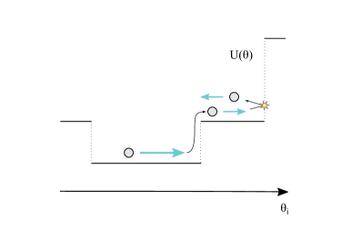
Figure 1: An example trajectory $\bm{\theta}(t)$ of discontinuous Hamiltonian dynamics. The trajectory has enough kinetic energy to move across the first discontinuity by transferring some kinetic energy to potential energy. Across the second discontinuity, however, the trajectory has insufficient kinetic energy to compensate for the potential energy increase and bounces back as a result.

By emulating the behavior of the solution $\{\bm{\theta}(t),\bm{p}(t)\}$, we obtain an efficient integrator of the coordinate-wise equation (12) as given in Algorithm 1. While the parameter $\bm{\theta}$ does not get updated when $m_{i}^{-1}|p_{i}|<\Delta U$ (line 1), the momentum flip $p_{i}\leftarrow-p_{i}$ (line 1) ensures that the next numerical integration step leads the trajectory toward a higher density of $\pi_{\Theta}(\bm{\theta})$. This can be viewed as a generalization of the guided random walk idea by Gustafson (1998).

The solution of the original (unsplit) differential equation (10) is approximated by sequentially updating each coordinate of $(\bm{\theta},\bm{p})$ with Algorithm 1 as illustrated in Figure 2. The reversibility of the resulting proposal is guaranteed by randomly permuting the order of the coordinate updates. Alternatively, one can split the operator symmetrically to obtain a reversible integrator (McLachlan & Quispel, 2002). The integrator does not reproduce the exact solution but nonetheless preserves the Hamiltonian exactly. This remains true with any stepsize $\epsilon$, but for good mixing the stepsize needs to be chosen small enough that the condition on Line 1 is satisfied with high probability (supplement Section S5).

3.4 Mixing momentum distributions for continuous and discrete parameters

The potential energy $U(\bm{\theta})$ is a smooth function of $\theta_{i}$ if both the prior and likelihood depend smoothly on $\theta_{i}$. The coordinate-wise update of Algorithm 1 leads to a valid proposal mechanism whether or not $U(\bm{\theta})$ has discontinuities along $\theta_{i}$. If $U(\bm{\theta})$ varies smoothly along some coordinates of $\bm{\theta}$, however, we can devise an integrator that takes advantage of the smooth dependence.

We first write $\bm{\theta}=(\bm{\theta}_{I},\bm{\theta}_{J})$ where the collections of indices $I$ and $J$ are defined as

$$I =\left\{i\in\{1,\ldots,d\}:\text{$U(\bm{\theta})$ is a smooth function of $\theta_{i}$}\right\},\quad J=\{1,\ldots,d\}\setminus I.$$ (16)

1 Function CoordIntegrator $(\bm{\theta},\bm{p},i,\epsilon)$:

2       $\bm{\theta}^{*}\leftarrow\bm{\theta}$

3       $\theta^{*}_{i}\leftarrow\theta^{*}_{i}+\epsilon m_{i}^{-1}\textrm{sign}(p_{i})$

4       $\Delta U\leftarrow U(\bm{\theta}^{*})-U(\bm{\theta})$

5       if $m_{i}^{-1}|p_{i}|>\Delta U$  then

6             $\theta_{i}\leftarrow\theta_{i}^{*}$

7             $p_{i}\leftarrow p_{i}-\textrm{sign}(p_{i})m_{i}\Delta U$

8            

9      else

10             $p_{i}\leftarrow-p_{i}$

11            

12      return $\bm{\theta},\,\bm{p}$

Algorithm 1 Coordinate-wise integrator for dynamics with Laplace momentum

Function DiscIntegrator $\left(\bm{\theta},\bm{p},\epsilon,\varphi=\textnormal{{Permute}}(J)\right)$:

       $\bm{p}_{I}\leftarrow\bm{p}_{I}+\dfrac{\epsilon}{2}\nabla_{\bm{\theta}_{I}}\log\pi(\bm{\theta})$

       $\bm{\theta}_{I}\leftarrow\bm{\theta}_{I}+\dfrac{\epsilon}{2}\,\bm{M}_{I}^{-1}\bm{p}_{I}$

       for $j\ \mathrm{in}\ J$ do

             $\bm{\theta},\,\bm{p}\leftarrow\textnormal{{CoordIntegrator}}(\bm{\theta},\bm{p},\varphi(j),\epsilon)$ // Update discontinuous params

            

      $\bm{\theta}_{I}\leftarrow\bm{\theta}_{I}+\dfrac{\epsilon}{2}\,\bm{M}_{I}^{-1}\bm{p}_{I}$

       $\bm{p}_{I}\leftarrow\bm{p}_{I}+\dfrac{\epsilon}{2}\nabla_{\bm{\theta}_{I}}\log\pi(\bm{\theta})$

       return $\bm{\theta},\,\bm{p}$

Algorithm 2 Integrator for discontinuous
Hamiltonian Monte Carlo

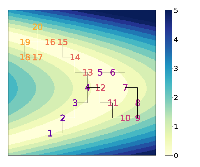
Figure 2: A trajectory of Laplace momentum based Hamiltonian dynamics $\{\theta_{1}(t),\theta_{2}(t)\}$ approximated by the coordinate-wise integrator of Algorithm 1. The log density of the target distribution changes in the increment of $0.5$ and has “banana-shaped” contours. Each numerical integration step consists of the coordinate-wise update along the horizontal axis followed by that along the vertical axis. The order of the coordinate updates is randomized at the beginning of numerical integration to ensure reversibility. The trajectory initially travels in the direction of the initial momentum, a process marked by the numbers 1 – 5. At the 5th numerical integration step, however, the trajectory does not have sufficient kinetic energy to take a step upward and hence flips the momentum downward. Such momentum flips also occur at the 8th and 9th numerical integration steps, again changing the direction of the trajectory. The rest of the trajectory follows the same pattern.

More precisely, we assume that the parameter space has a partition $\mathbb{R}^{|I|}\times\mathbb{R}^{|J|}=\cup_{k}\mathbb{R}^{|I|}\times\Omega_{k}$ such that $U(\bm{\theta})$ is smooth on $\mathbb{R}^{|I|}\times\Omega_{k}$ for each $k$. We write $\bm{p}=(\bm{p}_{I},\bm{p}_{J})$ correspondingly and define the distribution of $\bm{p}$ as a product of Gaussian and Laplace so that

$$K(\bm{p})=-\log\pi_{P}(\bm{p})=\frac{1}{2}\,\bm{p}_{I}^{\intercal}\bm{M}_{I}^{-1}\bm{p}_{I}+\textstyle{\sum}_{j\in J}m_{j}^{-1}|p_{j}|,$$ (17)

where $\bm{M}_{I}$ and $\bm{M}_{J}=\textrm{diag}(\bm{m}_{J})$ are mass matrices (Neal, 2010). With slight abuse of terminology, we will refer to $(\bm{\theta}_{J},\bm{p}_{J})$ as discontinuous parameters.

When mixing Gaussian and Laplace momenta, we approximate the dynamics via an integrator based again on operator splitting; we update the smooth parameter $(\bm{\theta}_{I},\bm{p}_{I})$ first, then the discontinuous parameter $(\bm{\theta}_{J},\bm{p}_{J})$, followed by another update of $(\bm{\theta}_{I},\bm{p}_{I})$. The discontinuous parameters are updated coordinate-wise as described in Section 3.3. The update of $(\bm{\theta}_{I},\bm{p}_{I})$ is based on a decomposition familiar from the leapfrog scheme:

$$\frac{\textrm{d}\bm{p}_{I}}{\textrm{d}t} =\nabla_{\bm{\theta}_{I}}\log\pi(\bm{\theta}),\quad \frac{\textrm{d}\bm{\theta}_{I}}{\textrm{d}t} =\bm{0},\quad \frac{\textrm{d}\bm{\theta}_{J}}{\textrm{d}t} =\frac{\textrm{d}\bm{p}_{J}}{\textrm{d}t}=\bm{0},$$ (18)

$$\frac{\textrm{d}\bm{\theta}_{I}}{\textrm{d}t} =\bm{M}_{I}^{-1}\bm{p}_{I},\ \frac{\textrm{d}\bm{p}_{I}}{\textrm{d}t} =\bm{0},\ \frac{\textrm{d}\bm{\theta}_{J}}{\textrm{d}t} =\frac{\textrm{d}\bm{p}_{J}}{\textrm{d}t}=\bm{0}.$$ (19)

Algorithm 2 describes the integrator with all the ingredients put together. When mixing in Gaussian momentum, the integrator continues to preserve the Hamiltonian accurately if not exactly, with the global error rate of $O(\epsilon^{2})$ (supplement Section S9). Advantages of separately treating continuous and discontinuous parameters in this manner are discussed in the supplement Section S4.

4 Theoretical properties of discontinuous Hamiltonian Monte Carlo

4.1 Reversibility of discontinuous Hamiltonian Monte Carlo transition kernel

As for existing Hamiltonian Monte Carlo variants, the reversibility of discontinuous Hamiltonian Monte Carlo is a direct consequence of the reversibility and volume-preserving property of our integrator in Algorithm 2 (Neal, 2010; Fang et al., 2014). We thus focus on establishing these properties of our integrator. Let $\bm{\Psi}$ denote a bijective map on the space $(\bm{\theta},\bm{p})$ corresponding to the approximation of discontinuous Hamiltonian dynamics through multiple numerical integration steps. An integrator is reversible if $\bm{\Psi}$ satisfies

$$(\bm{R}\circ\bm{\Psi})^{-1}=\bm{R}\circ\bm{\Psi}\quad\text{ or equivalently }\quad\bm{\Psi}^{-1}=\bm{R}\circ\bm{\Psi}\circ\bm{R},$$ (20)

where $\bm{R}:(\bm{\theta},\bm{p})\to(\bm{\theta},-\bm{p})$ is the momentum flip operator. Due to the updates of discrete parameters in a random order, the map $\bm{\Psi}$ induced by our integrator is non-deterministic. Consequently, our integrator has an unconventional feature of being reversible “in distribution” only, $(\bm{R}\circ\bm{\Psi})^{-1}\overset{d}{=}\bm{R}\circ\bm{\Psi}$, which is sufficient for the resulting Markov chain to be reversible.

Lemma 4.1.

For a piecewise smooth potential energy $U(\bm{\theta})$, the coordinate-wise integrator of Algorithm 1 is volume-preserving and reversible for any coordinate index $i$ except on a set of Lebesgue measure zero. Moreover, updating multiple coordinates with the integrator in a random order $\varphi(1),\ldots,\varphi(d)$ is again reversible in distribution provided that the random permutation $\varphi$ satisfies $\left\{\varphi(1),\varphi(2),\ldots,\varphi(d)\right\}\overset{d}{=}\{\varphi(d),\varphi(d-1),\ldots,\varphi(1)\}$.

Theorem 4.2.

For a piecewise smooth potential energy $U(\bm{\theta})$, the integrator of Algorithm 2 is volume-preserving and reversible except on a set of Lebesgue measure zero.

The proofs are in the supplement Section S6. In the same section, we also establish the reversibility and volume-preserving property of discontinuous Hamiltonian dynamics under alternative kinetic energies.

4.2 Irreducibility via randomized stepsize

Reducible behaviors in Hamiltonian Monte Carlo are rarely observed in practice despite the subtleties in theoretical analysis (Livingstone et al., 2016; Bou-Rabee et al., 2017; Durmus et al., 2017). However, care needs to be taken when applying the coordinate-wise integrator for discontinuous Hamiltonian Monte Carlo; its use with a fixed stepsize $\epsilon$ results in a reducible Markov chain which is not ergodic. To see the issue, consider the transition probability of multiple iterations of discontinuous Hamiltonian Monte Carlo based on the integrator of Algorithm 2. Given the initial state $\bm{\theta}_{0}$, the integrator of Algorithm 1 moves the $i$-th coordinate of $\bm{\theta}$ only by the distance $\pm\epsilon m_{i}^{-1}$ regardless of the values of the momentum variable. The transition probability in the $\bm{\theta}$-space with $\bm{p}$ marginalized out, therefore, is supported on a grid

$$\Omega=\left\{(\bm{\theta}_{I},\bm{\theta}_{J}):\bm{\theta}_{J}=\bm{\theta}_{0,J}+\epsilon\bm{m}\odot\bm{k}\text{ for a vector of integers $\bm{k}$}\right\},$$ (21)

where $\bm{\theta}_{J}$ as in (16) denotes the coordinates of $\bm{\theta}$ with discontinuous conditionals.

This pathological behavior can be avoided by randomizing the stepsize at each iteration, say $\epsilon\sim\textrm{Unif}(\epsilon_{\min},\epsilon_{\max})$. Randomizing the stepsize additionally addresses a possibility that smaller stepsizes are required in some regions of the parameter space (Neal, 2010). While the coordinate-wise integrator does not suffer from the stability issue of the leapfrog scheme, the quantity $\epsilon m_{i}^{-1}$ nonetheless needs to match the length scale of $\theta_{i}$; see the supplement Section S5.

4.3 Metropolis-within-Gibbs with momentum as special case

Consider a version of discontinuous Hamiltonian Monte Carlo in which all the parameters are updated with the coordinate-wise integrator of Algorithm 1; in other words, the integrator of Algorithm 2 is applied with $J=\{1,\ldots,d\}$ and an empty indexing set $I$. This version is a generalization of random-scan Metropolis-within-Gibbs, also known as one-variable-at-a-time Metropolis. We therefore refer to this version as Metropolis-within-Gibbs with momentum.

We use $\pi_{\mathcal{E}}(\cdot)$ and $\pi_{\Phi}(\cdot)$ to denote the distribution of a stepsize $\epsilon$ and of a permutation $\varphi$ of $\{1,\ldots,d\}$, where $\pi_{\Phi}(\cdot)$ satisfies $\left\{\varphi(1),\ldots,\varphi(d)\right\}\overset{d}{=}\{\varphi(d),\ldots,\varphi(1)\}$. With these notations, each iteration of Metropolis-within-Gibbs with momentum can be expressed as follows:

1. Draw $\epsilon\sim\pi_{\mathcal{E}}(\cdot)$, $\varphi\sim\pi_{\Phi}(\cdot)$, and $p_{j}\sim\textrm{Laplace}(\textrm{scale}=m_{j})$ for $j=1,\ldots,d$.

2. Repeat for $L$ times a sequential update of the coordinate $(\theta_{j},p_{j})$ for $j=\varphi(1),\ldots,\varphi(d)$ via Algorithm 1 with stepsize $\epsilon$.

In this version of discontinuous Hamiltonian Monte Carlo, the integrator exactly preserves the Hamiltonian and the acceptance-rejection step can be omitted.

When $L=1$, the above algorithm recovers random-scan Metropolis-within-Gibbs. This can be seen by realizing that Lines 1 – 1 of Algorithm 1 coincide with the standard Metropolis acceptance-rejection procedure for $\theta_{j}$. More precisely, the coordinate-wise integrator updates $\theta_{j}$ to $\theta_{j}+\epsilon m_{j}^{-1}\textrm{sign}(p_{j})$ only if

$$\exp\!\left\{-U(\bm{\theta}^{*})+U(\bm{\theta})\right\}>\exp\big{(}-m_{j}^{-1}|p_{j}|\big{)}\overset{d}{=}\textrm{Unif}(0,1),$$ (22)

where the last distributional equality follows from the fact $m_{j}^{-1}|p_{j}|\overset{d}{=}\textrm{Exp}(1)$. To summarize, when taking only one numerical integration step, the version of discontinuous Hamiltonian Monte Carlo considered here coincides with Metropolis-within-Gibbs with a random scan order $\varphi\sim\pi_{\Phi}(\cdot)$ and a symmetric proposal $\theta_{j}\pm\epsilon m_{j}^{-1}$ for each parameter with $\epsilon\sim\pi_{\mathcal{E}}(\cdot)$. We could also consider a version of discontinuous Hamiltonian Monte Carlo with a fixed stepsize $\epsilon=1$ but with a mass matrix randomized $(m_{1}^{-1},\ldots,m_{d}^{-1})\sim\pi_{M^{-1}}(\cdot)$ before each numerical integration step; this version would correspond to a more standard Metropolis-within-Gibbs with independent univariate proposals.

Being a generalization of Metropolis-within-Gibbs, discontinuous Hamiltonian Monte Carlo is guaranteed a superior performance:

Corollary 4.3.

Under any efficiency metric, which may account for computational costs per iteration, an optimally tuned discontinuous Hamiltonian Monte Carlo is guaranteed to outperform a class of random-scan Metropolis-within-Gibbs samplers as described above.

In particular, an optimally tuned discontinuous Hamiltonian Monte Carlo will inherit the geometric ergodicity of a corresponding Metropolis-within-Gibbs sampler, sufficient conditions for which are investigated in Johnson et al. (2013). In practice, the addition of momentum to Metropolis-within-Gibbs allows for a more efficient update of correlated parameters as empirically confirmed in the supplement Section S8.1.

Besides being a generalization Metropolis-within-Gibbs, discontinuous Hamiltonian Monte Carlo has a curious connection to the zig-zag sampler, a state-of-the-art non-reversible Monte Carlo algorithm. The Laplace-momentum based Hamiltonian dynamics exhibits behaviors remarkably similar to the piece-wise deterministic Markov process underlying the zig-zag sampler (supplement Section S6.4).

5 Numerical results

5.1 Experimental set-up, benchmarks, and efficiency metric

We use two challenging posterior inference problems to demonstrate the efficiency of discontinuous Hamiltonian Monte Carlo as a general-purpose sampler. Additional numerical results in the supplement Section S8 further illustrate the breadth of its capability. Codes to reproduce the simulation results are available at https://github.com/aki-nishimura/discontinuous-hmc.

Few general and efficient approaches currently exist for sampling from a discrete parameter or a discontinuous target density. For each problem, therefore, we pick a few most appropriate general-purpose samplers to benchmark against. Chopin & Ridgway (2017) compare a variety of algorithms on posterior distributions of binary classification problems. One of their conclusions is that, while random-walk Metropolis is known to scale poorly in the number of parameters (Roberts et al., 1997), Metropolis with a properly adapted proposal covariance is competitive with alternatives even in a 180-dimensional space. As one of our benchmarks, therefore, we use random-walk Metropolis with proposal covariances proportional to estimated target covariances (Roberts et al., 1997; Haario et al., 2001). When the conditional densities can be evaluated efficiently and no strong dependence exists among the parameters, Metropolis-within-Gibbs with component-wise adaptation can scale better than joint sampling via random-walk Metropolis (Haario et al., 2005). This approach thus is used as another benchmark.

For models with discrete parameters, we also compare with the No-U-turn / Gibbs approach (Salvatier et al., 2016). Conditionally on discrete parameters, continuous parameters are updated by the no-U-turn sampler of Hoffman & Gelman (2014). The standard implementation then updates discrete parameters with univariate Metropolis, but here we implement full conditional univariate updates via manually-optimized multinomial samplings. In our examples, these multinomial samplings take little time relative to continuous parameter updates, tilting the comparison in favor of No-U-turn / Gibbs. We use the identity mass matrix for the no-U-turn sampler to make a fair comparison to discontinuous Hamiltonian Monte Carlo with the identity mass.

In all our numerical results, continuous parameters with range constraints are transformed into unconstrained ones to facilitate sampling. More precisely, the constraint $\theta>0$ is handled by a log transform $\theta\to\log\theta$ and $\theta\in[0,1]$ by a logit transform $\theta\to\log\left\{\theta/(1-\theta)\right\}$ as done in Stan and PyMC (Stan Development Team, 2016; Salvatier et al., 2016). For each example, the stepsize and path length for discontinuous Hamiltonian Monte Carlo were manually adjusted over short preliminary runs by visually examining trace plots. The stepsize for the continuous parameter updates of No-U-turn / Gibbs was adjusted analogously.

Efficiencies of the algorithms are compared through effective sample sizes (Geyer, 2011). As is commonly done in the Markov chain Monte Carlo literature, we compute the effective sample sizes of the first and second moment estimators for each parameter and report the minimum value across all the parameters. Effective sample sizes are estimated using the method of batch means with 25 batches (Geyer, 2011), averaged over the estimates from 8 independent chains.

5.2 Jolly-Seber model: estimation of unknown open population size and survival rate from multiple capture-recapture data

The Jolly-Seber model and its extensions are widely used in ecology to estimate unknown population sizes along with related parameters of interest (Schwarz & Seber, 1999). The model is motivated by the following experimental design. Individuals from a particular species are captured, marked, and released back to the environment. This procedure is repeated over multiple capture occasions. At each occasion, the number of marked and unmarked individuals among the captured ones are recorded. Individuals survive from one capture occasion to another with an unknown survival rate. The population is assumed to be “open” so that individuals may enter, either through birth or immigration, or leave the area under study.

In order to be consistent with the literature on capture-recapture models, the notations within this section will deviate from the rest of the paper. Assuming that data are collected over $i=1,\ldots,T$ capture occasions, the unknown parameters are $\{U_{i},p_{i}\}_{i=1}^{T}$ and $\{\phi_{i}\}_{i=1}^{T-1}$, representing

$$U_{i} =\,\text{number of unmarked animals right before the $i$th capture occasion;}$$

$$p_{i} =\,\text{capture probability of each animal at the $i$th capture occasion;}$$

$$\phi_{i} =\,\text{survival probability of each animal from the $i$th to $(i+1)$th capture occasion.}$$

We assign standard objective priors $p_{i},\phi_{i}\sim\textrm{Unif}(0,1)$ and $\pi(U_{1})\propto U_{1}^{-1}$. The parameters $U_{2},\ldots,U_{T}$ require a more complex prior elicitation; this is described in the supplement Section S7 along with the likelihood function and other details on the Jolly-Seber model.

We take the black-kneed capsid population data from Jolly (1965) as summarized in Seber (1982). The data record the capture-recapture information over $T=13$ successive capture occasions, giving rise to a 38-dimensional posterior distribution involving 13 discrete parameters. We use the log-transformed embedding for the discrete parameter $U_{i}$’s (Section 2.2). The proposal covariance for random-walk Metropolis is chosen by pre-computing the true posterior covariance with a long adaptive Metropolis chain (Haario et al., 2001) and then scaling it according to Roberts et al. (1997). Discontinuous Hamiltonian Monte Carlo can also take advantage of the posterior covariance information, so we also try using a diagonal mass matrix whose entries are set according to the estimated posterior variance of each parameter (supplement Section S5). Starting from stationarity, we run $10^{4}$ iterations of discontinuous Hamiltonian Monte Carlo and No-U-turn / Gibbs and $5\times 10^{5}$ iterations of Metropolis.

The performance of each algorithm is summarized in Table 1 where “DHMC (diagonal)” and “DHMC (identity)” indicate discontinuous Hamiltonian Monte Carlo with a diagonal and identity mass matrix respectively. The table clearly indicates a superior performance over No-U-turn / Gibbs and Metropolis with approximately 60 and 7-fold efficiency increase respectively when using a diagonal mass matrix. The posterior distribution exhibits high negative correlations between $U_{i}$ and $p_{i}$ (Figure 4). All the algorithms record the worst effective sample size in $p_{1}$, but the mixing of No-U-turn / Gibbs suffers most as $U_{i}$ and $p_{i}$ are updated conditionally.

Table 1: Performance summary of each algorithm on the Jolly-Serber model example. “DHMC” and “ESS” in the table stand for discontinuous Hamiltonian Monte Carlo and effective sample size. The term $(\pm\ldots)$ indicates the error estimate, twice the standard deviations, of our effective sample size estimators. Path length is averaged over each iteration. “Iter time” shows the computational time per iteration of each algorithm relative to the fastest one.

	ESS per 100 samples	ESS per minute	Path length	Iter time
DHMC (diagonal)	45.5 ($\pm$ 5.2)	424	45	87.7
DHMC (identity)	24.1 ($\pm$ 2.6)	126	77.5	157
No-U-turn / Gibbs	1.04 ($\pm$ 0.087)	6.38	150	133
Metropolis	0.0714 ($\pm$ 0.016)	58.5	1	1

5.3 Generalized Bayesian belief update based on loss functions

Motivated by model misspecification and difficulty in modeling all aspects of a data generating process, Bissiri et al. (2016) propose a generalized Bayesian framework, which replaces the log-likelihood with a surrogate based on a utility function. Given an additive loss $\ell(y,\bm{\theta})$ for the data $y$ and parameter of interest $\bm{\theta}$, the prior $\pi(\bm{\theta})$ is updated to obtain the generalized posterior:

$$\pi_{\textrm{post}}(\bm{\theta})\propto\exp\!\left\{-\ell(\bm{y},\bm{\theta})\right\}\pi(\bm{\theta}).$$ (23)

While (23) coincides with a pseudo-likelihood type approach, Bissiri et al. (2016) derives the formula as a coherent and optimal update from a decision theoretic perspective.

Here we consider a binary classification problem with an error-rate loss:

$$\ell(\bm{y},\bm{\beta})=\textstyle{\sum}_{i=1}\mathbbm{1}\left\{y_{i}\bm{x}_{i}^{\intercal}\bm{\beta}<0\right\},$$ (24)

where $y_{i}\in\{-1,1\}$, $\bm{x}_{i}$ is a vector of predictors, and $\bm{\beta}$ is a regression coefficient. The target distribution of the form (23) based on the loss function (24) is suggested as a challenging test case by Chopin & Ridgway (2017). We use the SECOM data from the UCI machine learning repository, which records various sensor data that can be used to predict the production quality of a semi-conductor, measured as “pass” or “fail.” We first remove the predictors with more than 20 missing cases and then remove the observations that still had missing predictors, leaving 1,477 cases with 376 predictors. All the predictors are normalized and the regression coefficients $\beta_{i}$’s are given $\mathcal{N}(0,1)$ priors. Figure 4 illustrates the complexity of the target distribution.

Figure 3: The posterior marginal of $(p_{1},U_{1})$ with
parameter transformations, estimated from
the Monte Carlo samples.

Figure 4: The posterior conditional density of the intercept parameter in the generalized Bayes example. The other parameters are fixed at the posterior draw that recorded the highest posterior density among the Monte Carlo samples. The density is not continuous since the loss function is not.

In tuning the proposal covariance of Metropolis for this example, adaptive Metropolis performed so poorly that we instead use $10^{5}$ iterations of discontinuous Hamiltonian Monte Carlo to estimate the posterior covariance. Scaling the proposal covariance for random-walk Metropolis according to Roberts et al. (1997) resulted in an acceptance probability of less than 0.04, so we scaled the proposal covariance to achieve the acceptance probability of 0.234 with stochastic optimization (Andrieu & Thoms, 2008). We also found the posterior correlation to be very modest in this example, with the ratio of the largest to smallest eigenvalues of the estimated posterior covariance matrix being $46\approx 6.8^{2}$. This suggested that coordinate-wise updates may be competitive, so we implemented Metropolis-within-Gibbs as an additional benchmark. The parameters are updated one at a time with the acceptance rate calibrated around 0.44 as recommended in Gelman et al. (1996). We run discontinuous Hamiltonian Monte Carlo for $10^{4}$ iterations, Metropolis for $10^{7}$ iterations, and Metropolis-within-Gibbs for $5\times 10^{4}$ iterations from stationarity.

Table 2 summarizes the performance of each algorithm. Discontinuous Hamiltonian Monte Carlo with identity mass matrix outperforms Metropolis and Metropolis-within-Gibbs by a factor of 330 and 2 respectively. Using a diagonal mass matrix yields only a minor improvement here as the posterior displays similar scales of uncertainty in all the parameters. The mixing of Metropolis suffers substantially from the dimensionality of the target. Conditional updates of Metropolis-within-Gibbs mix well in this example due to weak dependence among the parameters. On the other hand, as demonstrated in the example here and in Section 5.2, discontinuous Hamiltonian Monte Carlo not only scales well in the number of parameters but also efficiently handles distributions with strong correlations.

Table 2: Performance summary of each algorithm on the generalized Bayesian posterior example. “DHMC” and “ESS” in the table stand for discontinuous Hamiltonian Monte Carlo and effective sample size. The term $(\pm\ldots)$ is the error estimate of our effective sample size estimators. Path length is averaged over each iteration. “Iter time” shows the computational time for one iteration of each algorithm relative to the fastest one.

	ESS per 100 samples	ESS per minute	Path length	Iter time
DHMC (identity)	26.3 ($\pm$ 3.2)	76	25	972
Metropolis	0.00809 ($\pm$ 0.0018)	0.227	1	1
Metropolis-within-Gibbs	0.514 ($\pm$ 0.039)	39.8	1	36.2

Supplement to “Discontinuous Hamiltonian Monte Carlo for discrete parameters and discontinuous likelihoods”

S1 Behavior of leapfrog integrator on discontinuous target

As mentioned in Section 2.3, in the presence of discontinuity, the leapfrog integrator in general incurs unbounded errors that do not decrease even as $\epsilon\to 0$. To see this, consider a discontinuous target $\pi_{c}(\theta)$ which is continuously differentiable except at $\theta=0$, is constant on $\theta\in[-\delta,0)\cup(0,\delta]$, and satisfies $\log\pi_{c}(-\delta)-\log\pi_{c}(\delta)=c>0$. In particular, we have $\nabla\log\pi_{c}(\theta)=0$ for $0<|\theta|<\delta$ and hence the leapfrog trajectory evolves with a constant momentum on $\theta\in[-\delta,\delta]$. In other words,

$$\theta(n\epsilon)=\theta_{0}+n\epsilon p_{0},\ \ p(n\epsilon)=p_{0},$$

provided $|\theta_{0}+k\epsilon p_{0}|<\delta$ for all $k=0,1,\ldots,n$. Starting from $\theta_{0}<0$, when the leapfrog trajectory crosses $\theta=0$ so that $\theta(k\epsilon)<0<\theta\{(k+1)\epsilon\}$, it incurs the error of

$$H\!\left[\theta\{(k+1)\epsilon\},p\{(k+1)\epsilon\}\right]-H\!\left\{\theta(k\epsilon),p(k\epsilon)\right\}$$

$$\hskip 80.00012pt=-\log\pi_{c}[\theta\{(k+1)\epsilon\}]+\log\pi_{c}\{\theta(k\epsilon)\}=c.$$

S2 Integrator for Gaussian momentum-based discontinuous dynamics

Here we describe an implementation of the integrator proposed by Pakman & Paninski (2013) and Afshar & Domke (2015). The integrator is designed to approximate a discontinuous Hamiltonian dynamics with a Gaussian momentum corresponding to the kinetic energy $K(\bm{p})=\|\bm{p}\|^{2}/2$. For simplicity, we assume that a parameter space $\Theta$ consists only of the embedded discrete parameters as described in Section 2.2, so that the target $\pi_{\Theta}(\cdot)$ is piecewise constant with the discontinuity set consisting of the boundaries of hyper-cubes. The integrator is energy-preserving in this simplified setting but not so for more general discontinuous dynamics. The pseudo code is given in Algorithm 3.

Input :  initial state $(\bm{\theta},\bm{p})$, stepsize $\epsilon$

$t\leftarrow 0$

while $t<\epsilon$ do

       $t_{e}\leftarrow$ the time until reaching the next discontinuity

       if $t+t_{e}>\epsilon$ then

             $\bm{\theta}\leftarrow\bm{\theta}+(\epsilon-t)\bm{p}$

             $t\leftarrow\epsilon$

            

      else

             $\bm{\theta}\leftarrow\bm{\theta}+t_{e}\bm{p}$

             $i\leftarrow$ the index of the axis orthogonal to the discontinuity plane at $\bm{\theta}$

             $\Delta U_{e}\leftarrow$ the potential energy difference

             if $p_{i}^{2}/2>\Delta U_{e}$ then

                   $p_{i}\leftarrow\sqrt{p_{i}^{2}-2\Delta U_{e}}$

                  

            else

                   $p_{i}\leftarrow-p_{i}$

                  

            $t\leftarrow t+t_{e}$

Algorithm 3 Integrator for Gaussian momentum-based discontinuous dynamics

S3 Empirical verification of ergodicity and unbiasedness of discontinuous Hamiltonian Monte Carlo

To empirically back up the theoretical results of Section 4, here we use discontinuous Hamiltonian Monte Carlo to sample from a simple posterior distribution with closed-form marginal distributions. The correctness of discontinuous Hamiltonian Monte Carlo has been independently verified by Gram-Hansen et al. (2018), in which the discontinuous Hamiltonian Monte Carlo samples are compared to the outputs of existing probabilistic programming softwares.

We consider an observation model $y\,|\,q,N\sim\mathrm{Binomial}(q,N)$ where both the success rate $q$ and sample size $N$ are unknown. We assign an objective prior $\pi(N)\propto N^{-1}$ (Berger et al., 2012) and a beta prior $q\sim\textrm{Beta}(\alpha,\beta)$. As the particular choice is immaterial for the purpose of our simulation, we just pick $\alpha=\beta=2$ and set $y=100$. Closed-form expressions for the posterior marginals of $N$ and $q$ are given in Section S3.1 below.

To sample from the posterior, we use the log-transformed embedding of $N$ (Section 2.2). The parameter $q$ is mapped to the real line through a logit transform $q\to\log\{q/(1-q)\}$. We use the integrator of Section 3.4 (Algorithm 2) with the Laplace momentum for $N$ and Gaussian momentum for $q$. The stepsize $\epsilon$ is jittered in the range $[0.08,0.1]$ and the number of numerical integration steps in the range $[15,20]$.

Figure S1 shows the empirical distributions of $N\,|\,y$ and $q\,|\,y$ from $10^{6}$ iterations of discontinuous Hamiltonian Monte Carlo. The empirical distributions are indistinguishable from the exact distributions indicated by the orange lines. Additionally, the trace plot in Figure S2 shows that discontinuous Hamiltonian Monte Carlo can induce a large transition in the parameter $N$ with only a small number of numerical integration steps. This means that the discontinuous Hamiltonian Monte Carlo integrator often jumps through a large number of discontinuities along the parameter $N$ at each numerical integration step. This behavior introduces no bias as the integrator remains reversible and volume-preserving regardless of its stepsize as discussed in the main manuscript Section 4.

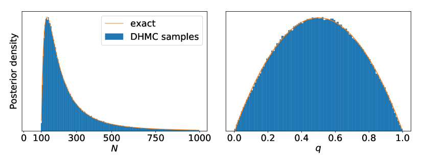
Figure S1: Empirical distributions of the discontinuous Hamiltonian Monte Carlo samples generated for the target distribution as described in Section S3.1. The orange lines show the exact posterior mass and density functions computed from the closed-form expressions. The unknown sample size parameter $N$ has no posterior probability below the observed number of successes $y=100$.

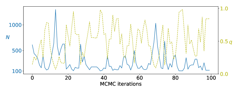
Figure S2: Trace plots for the first 100 discontinuous Hamiltonian Monte Carlo samples generated for the target distribution as described in Section S3.1. The blue line and left $y$-axis indicates the parameter values of $N$, while the olive line and right $y$-axis indicates the parameter values of $q$.

S3.1 Derivation of the posterior marginals

For the model and priors described above, we have

$$\pi(N,q\,|\,y) \propto\frac{N!}{(N-y)!}q^{y}(1-q)^{N-y}\pi(q)\pi(N)\propto\frac{(N-1)!}{(N-y)!}q^{y+\alpha-1}(1-q)^{N-y+\beta-1}$$ (S1)

Integrating over $q$, we obtain

$$\pi(N\,|\,y) \propto\frac{(N-1)!}{(N-y)!}\frac{\Gamma(N-y+\beta)}{\Gamma(N+\alpha+\beta)}=\frac{(N-1)!}{(N-y)!}\frac{(N-y+\beta-1)!}{(N+\alpha+\beta-1)!}$$ (S2)

where the equality holds when $\alpha$ and $\beta$ take positive integer values. The choice $\alpha=\beta=2$ yields

$$\pi(N\,|\,y) \propto\frac{N-y+1}{(N+3)(N+2)(N+1)N}$$ (S3)

We can compute the normalized mass function of $N\,|\,y$ to high accuracy by truncating it at a suitably large number. Having computed $\pi(N\,|\,y)$, we can compute the posterior marginal of $q$ via the law of total expectation $\pi(q\,|\,y)=\sum_{N}\pi(q\,|\,N,y)\pi(N\,|\,y)$ where $q\,|\,N,y\sim\mathrm{Beta}(y+\alpha,N-y+\beta)$.

S4 Relative advantages of joint and coordinate-wise updates on continuous parameters

While the coordinate-wise update of Algorithm 1 in the main manuscript generates a valid proposal whether or not $U(\bm{\theta})$ has discontinuities along $\theta_{i}$, the joint update of continuous parameters as in Algorithm 2 has some computational advantages. First, when there is little conditional independence structure, calculating $\nabla_{\bm{\theta}_{I}}U(\bm{\theta})$ is more computationally efficient than carrying out $|I|$ successive conditional density evaluations. Even when there is some conditional independence structure, however, computing $\nabla_{\bm{\theta}_{I}}U(\bm{\theta})$ may still be substantially faster as an interpreter or compiler of a programing language can more easily optimize the required computation. Thus the joint update typically demands less computing time. On the other hand, the coordinate-wise updates have an advantage of being rejection-free by virtue of exact energy-preservation. The coordinate-wise update may thus be preferable for posteriors with substantial conditional independence structure such as those in latent Markov random field models.

S5 Tuning mass matrix and integrator stepsize of discontinuous Hamiltonian Monte Carlo

S5.1 Role and tuning of mass matrix

As in the case of traditional Hamiltonian Monte Carlo, using a non-identity mass matrix has the effect of preconditioning a target distribution through reparametrization (Neal, 2010). More precisely, for a matrix $\bm{A}_{I}$ and a diagonal matrix $\bm{A}_{J}$, the performance of discontinuous Hamiltonian Monte Carlo under parametrization $(\bm{A}_{I}\bm{\theta}_{I},\bm{A}_{J}\bm{\theta}_{J},\bm{p}_{I},\bm{p}_{J})$ is identical to that for $(\bm{\theta}_{I},\bm{\theta}_{J},\bm{A}_{I}^{\intercal}\bm{p}_{I},\bm{A}_{J}^{\intercal}\bm{p}_{J})$. The choice of a mass matrix for a Gaussian momentum is a well-studied topic (Neal, 2010; Girolami & Calderhead, 2011). We can reason similarly for a Laplace momentum. We generally expect that sampling is facilitated by a reparametrization $\theta_{j}\to\theta_{j}/\textrm{var}(\theta_{j})^{1/2}$ for $j\in J$. This is effectively achieved, given the relation between mass matrix choice and parameter transformation, by choosing the mass to be $m_{j}\approx\textrm{var}(\theta_{j})^{-1/2}$. The variances can be estimated from a small number of preliminary discontinuous Hamiltonian Monte Carlo iterations.

While the above discussion focuses on a diagonal mass matrix, it is also possible to encode the correlation structure of the target distribution into the Laplace momentum $p_{J}$. To precondition $\theta_{J}$ by reparametrization $\theta_{J}\to\bm{M}_{J}^{-1/2}\theta_{J}$, we can define the distribution of $p_{J}$ to have independent Laplace distributions along the eigenvectors $u_{1},\ldots,u_{k}$ of $\bm{M}_{J}$:

$$p_{J}=\textstyle\sum_{j}\tilde{p}_{j}u_{j}\ \text{ for }\,\tilde{p}_{j}\sim\text{Laplace}(\text{scale}=\delta_{j}),$$ (S4)

so that $\text{Var}(p_{J})=\bm{M}_{J}=UDU^{\text{\raisebox{1.50694pt}{$\intercal$}}}$ where $U=[u_{1}|\ldots|u_{k}]$ and $D=\text{diag}(\delta_{1},\ldots,\delta_{k})$. The coordinate-wise integrator of Algorithm 1 can then be applied along each $u_{j}$ one at a time. The new coordinate is likely to break the original conditional independence structures among the parameters, however, making each coordinate-wise update more expensive. To incorporate a correlation structure while preserving some of the conditional independence structure, one possibility is to choose a block-diagonal $\bm{M}_{J}$.

S5.2 Choice and tuning of integrator stepsize

The stepsize $\epsilon$ should be adjusted so that $\epsilon m_{j}^{-1}$ has the same order of magnitude as a typical scale of the conditional distribution of $\theta_{j}$. Unlike a leapfrog integrator that becomes unstable as $\epsilon$ increases, the coordinate-wise integrator remains exactly energy-preserving but at some point a large stepsize will cause discontinuous Hamiltonian Monte Carlo to “get stuck” at the current state. The numerical integration scheme of discontinuous Hamiltonian Monte Carlo will keep flipping the momentum $p_{j}\leftarrow-p_{j}$ (Line 1 of Algorithm 1) without updating $\theta_{j}$ until the following condition is met:

$$U\big{\{}\bm{\theta}+\epsilon m_{j}^{-1}\textrm{sign}(p_{j})\bm{e}_{j}\big{\}}-U(\bm{\theta})<m_{j}^{-1}|p_{j}|\overset{d}{=}\textrm{Exponential}(1),$$ (S5)

where $\bm{e}_{j}$ denotes the $j$-th standard basis vector. When $\epsilon m_{j}^{-1}$ becomes larger than a typical scale of $\theta_{j}$, the condition (S5) becomes unlikely to be satisfied, leading to infrequent updates of $\theta_{j}$.

We now consider how to tune the stepsize while the mass matrix fixed. This can be alternated with tuning of the mass matrix as suggested above to calibrate both the tuning parameters. To this end, we propose the following statistics:

$$\mathbb{P}_{\pi_{\Theta}\times\pi_{P}}\left[U\big{\{}\bm{\theta}+\epsilon m_{j}^{-1}\textrm{sign}(p_{j})\bm{e}_{j}\big{\}}-U(\bm{\theta})>m_{j}^{-1}|p_{j}|\right]$$ (S6)

$$\hskip 30.00005pt=\mathbb{E}_{\pi_{\Theta}\times\pi_{P}}\left\{\min\left(1,\,\exp\Big{[}U(\bm{\theta})-U\big{\{}\bm{\theta}+\epsilon m_{j}^{-1}\textrm{sign}(p_{j})\bm{e}_{j}\big{\}}\Big{]}\right)\right\}.$$

The above statistics play a role analogous to the acceptance rate of Metropolis proposals. The statistics (S6) can be estimated, for example, by counting the frequency of momentum flips during each discontinuous Hamiltonian Monte Carlo iteration, and can then be used to tune the stepsize through stochastic optimization (Andrieu & Thoms, 2008; Hoffman & Gelman, 2014). One would want the statistics to be well above zero but not too close to 1, balancing the mixing rate and computational cost of each discontinuous Hamiltonian Monte Carlo iteration. Theoretical analysis of the optimal statistics value is beyond the scope of this paper, but the value 0.7 $\sim$ 0.9 is perhaps reasonable in analogy with the optimal acceptance rate for Hamiltonian Monte Carlo (Betancourt et al., 2014).

S6 Theoretical properties of discontinuous Hamiltonian Monte Carlo: proofs and additional results

S6.1 Proof of Lemma 4.1 and Theorem 4.2

Proof S6.1 (Lemma 4.1).

Assume $p_{i}\neq 0$ for now and let $\bm{e}_{i}$ denote the $i$th standard basis vector. Then one step of Algorithm 1 corresponds to a map $\bm{\Psi}_{i,\epsilon}:(\bm{\theta},\bm{p})\to(\bm{\theta}^{*},\bm{p}^{*})$ where

$$\bm{\theta}^{*}=\bm{\theta}+\epsilon m_{i}^{-1}\textrm{sign}(p_{i})\bm{e}_{i},\quad\bm{p}^{*}=\bm{p}-m_{i}\left\{U(\bm{\theta}^{*})-U(\bm{\theta})\right\}\bm{e}_{i}$$ (S7)

if $U\{\bm{\theta}+\epsilon m_{i}^{-1}\textrm{sign}(p_{i})\bm{e}_{i}\}-U(\bm{\theta})>m_{i}^{-1}p_{i}$, and otherwise

$$\bm{\theta}^{*}=\bm{\theta},\quad\bm{p}^{*}=-\bm{p}.$$ (S8)

The update equations (S7) and (S8) are well-defined and differentiable except on the measure-zero set $S$, which we define momentarily. Under both (S7) and (S8), we have $\partial\bm{\theta}^{*}/\partial\bm{p}=0$ and can easily show that

$$\det\left\{\frac{\partial(\bm{\theta}^{*},\bm{p}^{*})}{\partial(\bm{\theta},\bm{p})}\right\}=\det\left(\frac{\partial\bm{\theta}^{*}}{\partial\bm{\theta}}\right)\det\left(\frac{\partial\bm{p}^{*}}{\partial\bm{p}}\right)=1,$$ (S9)

establishing the volume-preservation. The reversibility as defined in (20) can be directly verified by solving the update equations (S7) and (S8) for $(\bm{\theta},-\bm{p})$ as a function of $(\bm{\theta}^{*},-\bm{p}^{*})$.

We now quantify the set $S$ on which the above argument may break down and show that it has measure zero. Let $\mathcal{D}$ denote the discontinuity set of $U(\bm{\theta})$ and $\mathcal{D}+\bm{v}$ denote a set of points in $\mathcal{D}$ shifted by a vector $\bm{v}$. It is easy to see that the update equations (S7) and (S8) are well-defined and differentiable except when $(\bm{\theta},\bm{p})$ belongs to one of the sets below:

$$\mathcal{D}\times\mathbb{R}^{d},\ \left(\mathcal{D}\pm\epsilon m_{i}^{-1}\bm{e}_{i}\right)\times\mathbb{R}^{d},\ \left\{p_{i}=0\right\},\ \left\{U\{\bm{\theta}+\epsilon m_{i}^{-1}\textrm{sign}(p_{i})\bm{e}_{i}\}-U(\bm{\theta})=m_{i}^{-1}p_{i}\right\}.$$ (S10)

Each of these sets above corresponds to lower-dimensional manifolds of the parameter space and hence have measure zero. We define the set $S$ as the union of all the sets (S10) over $i=1,\ldots,d$. Being a finite union of measure-zero sets, the set $S$ also has measure zero.

Lastly, we prove the reversibility of multiple coordinate updates corresponding to a map $\bm{\Psi}_{\varphi(d),\epsilon}\circ\ldots\circ\bm{\Psi}_{\varphi(1),\epsilon}$ with a random permutation $\varphi$. From the reversibility of each $\bm{\Psi}_{i,\epsilon}$, we deduce that

$$\bm{R}\circ\left(\bm{\Psi}_{\varphi(d),\epsilon}\circ\ldots\circ\bm{\Psi}_{\varphi(1),\epsilon}\right)\circ\bm{R} =\bm{\Psi}_{\varphi(d),\epsilon}^{-1}\circ\ldots\circ\bm{\Psi}_{\varphi(1),\epsilon}^{-1}=\left(\bm{\Psi}_{\varphi(1),\epsilon}\circ\ldots\circ\bm{\Psi}_{\varphi(d),\epsilon}\right)^{-1}.$$ (S11)

By our assumption on the distribution of $\varphi$, we have

$$\left(\bm{\Psi}_{\varphi(1),\epsilon}\circ\ldots\circ\bm{\Psi}_{\varphi(d),\epsilon}\right)^{-1}\overset{d}{=}\left(\bm{\Psi}_{\varphi(d),\epsilon}\circ\ldots\circ\bm{\Psi}_{\varphi(1),\epsilon}\right)^{-1}$$ (S12)

establishing the reversibility of $\bm{\Psi}_{\varphi(d),\epsilon}\circ\ldots\circ\bm{\Psi}_{\varphi(1),\epsilon}$ in distribution.

Proof S6.2 (Theorem 4.2).

Let $\bm{\Psi}_{J,\,\varphi,\,\epsilon}=\bm{\Psi}_{\varphi(d^{\prime}),\,\epsilon}\circ\ldots\circ\bm{\Psi}_{\varphi(1),\,\epsilon}$ where $\bm{\Psi}_{j,\epsilon}:(\bm{\theta},\bm{p})\to(\bm{\theta}^{*},\bm{p}^{*})$ is defined as in (S7) and (S8) and $\varphi(1),\ldots,\varphi(d^{\prime})$ is a permutation of the indexing set $J$. Also define $\bm{\Psi}_{\Theta,\,I,\,\epsilon/2}$ and $\bm{\Psi}_{P,\,I,\,\epsilon/2}$ as a function of $(\bm{\theta},\bm{p})$ such that

$$\bm{\Psi}_{\Theta,\,I,\,\epsilon/2}:\bm{\theta}_{I}\to\bm{\theta}_{I}+\dfrac{\epsilon}{2}\,\bm{M}_{I}^{-1}\bm{p}_{I},\quad\bm{\Psi}_{P,\,I,\,\epsilon/2}:\bm{p}_{I}\to\bm{p}_{I}-\dfrac{\epsilon}{2}\nabla_{\bm{\theta}_{I}}U(\bm{\theta})$$ (S13)

while leaving all the other coordinates unchanged. The integrator of Algorithm 2 can then be formally expressed as a map

$$\bm{\Psi}_{\Theta,\,I,\,\epsilon/2}\circ\bm{\Psi}_{P,\,I,\,\epsilon/2}\circ\bm{\Psi}_{J,\,\varphi,\,\epsilon}\circ\bm{\Psi}_{P,\,I,\,\epsilon/2}\circ\bm{\Psi}_{\Theta,\,I,\,\epsilon/2}.$$ (S14)

Being a symmetric composition of reversible maps, the map (S14) is again reversible. The maps $\bm{\Psi}_{\Theta,\,I,\,\epsilon/2}\circ\bm{\Psi}_{P,\,I,\,\epsilon/2}$ and $\bm{\Psi}_{P,\,I,\,\epsilon/2}\circ\bm{\Psi}_{\Theta,\,I,\,\epsilon/2}$ coincide with symplectic Euler schemes in the coordinate $(\bm{\theta}_{I},\bm{p}_{I})$ and hence a
re volume preserving (Hairer et al., 2006). Since $\bm{\Psi}_{J,\,\varphi,\,\epsilon}$ is also volume-preserving by the results of Lemma 4.1, the composition (S14) is volume-preserving.

S6.2 Reversibility and volume-preserving property of discontinuous dynamics under alternative kinetic energies

In Theorem S6.3 below, we establish the reversibility and volume-preserving property of discontinuous Hamiltonian dynamics with alternative kinetic energies. Theorem S6.3 extends the result of Afshar & Domke (2015) and justifies the use of the Gaussian momentum-based integrator Algorithm 3 in the supplement. A solution operator $\bm{\Psi}_{t}$ of a differential equation, or more generally of a differential inclusion, is a map such that $\{\bm{\theta}(t),\bm{p}(t)\}=\bm{\Psi}_{t}(\bm{\theta}_{0},\bm{p}_{0})$ is a solution of the equation with the initial condition $\{\bm{\theta}(0),\bm{p}(0)\}=(\bm{\theta}_{0},\bm{p}_{0})$. Also, symplecticity is a property of Hamiltonian dynamics which implies volume-preservation. Section S6.3 below provides the definition of symplecticity as well as the proof of Theorem S6.3.

Theorem S6.3.

Let $U(\bm{\theta})$ be a piecewise constant potential energy function whose discontinuity set is piecewise linear. Suppose that a kinetic energy $K(\bm{p})$ is symmetric, convex, piecewise smooth, and satisfies the growth condition $K(\bm{p})\to\infty$ as $\|\bm{p}\|\to\infty$. Then the solution operator $\bm{\Psi}_{t}$ of discontinuous Hamiltonian dynamics as defined in Section 2.4 is symplectic and reversible except on a set of Lebesgue measure zero.

Theorem S6.3 generalizes the result of Afshar & Domke (2015) to a larger class of kinetic energies, but we believe the conclusions can be extended to an even larger class of potential and kinetic energies. Such results may prove useful in constructing alternative approaches for dealing with discontinuous targets.

S6.3 Symplecticity of discontinuous Hamiltonian dynamics

Here we establish the symplecticity of discontinuous Hamiltonian dynamics under the assumptions of Theorem S6.3. Symplecticity implies a volume preservation and further has important consequences in the stability of numerical approximation schemes (Hairer et al., 2006).

Definition S6.4.

A differentiable map $(\bm{\theta},\bm{p})\to(\bm{\theta}^{*},\bm{p}^{*})$ is called symplectic if

$$\frac{\partial(\bm{\theta}^{*},\bm{p}^{*})}{\partial(\bm{\theta},\bm{p})}^{T}\bm{J}\,\frac{\partial(\bm{\theta}^{*},\bm{p}^{*})}{\partial(\bm{\theta},\bm{p})}=\bm{J}\quad\text{ for }\bm{J}=\begin{bmatrix}0&\bm{I}_{d}\\ -\bm{I}_{d}&0\end{bmatrix},$$ (S15)

where $\bm{I}_{d}$ denotes a $d$-dimensional identity matrix. A dynamics is called symplectic if its solution operator is.

Proof S6.5 (of Theorem S6.3).

Reversibility is a standard property of smooth Hamiltonian dynamics with a symmetric kinetic energy (Hairer et al., 2006). Defined as a point-wise limit of smooth dynamics, discontinuous dynamics therefore is also reversible.

We turn to the proof of symplecticity. Under the assumption of Theorem S6.3, the evolution of discontinuous Hamiltonian dynamics from a state $(\bm{\theta},\bm{p})$ at $t=0$ to $(\bm{\theta}^{*},\bm{p}^{*})$ at $t=\tau$ is given as follows. Dividing up the time intervals into a smaller pieces if necessary, we can without loss of generality assume that a trajectory $\left\{\bm{\theta}(t),\bm{p}(t)\right\}$ encounters only one discontinuity at $\bm{\theta}(t_{e})$ during the interval $[0,\tau]$. Since $U(\bm{\theta})$ is piecewise constant, the momentum remains constant and $\bm{\theta}(t)$ travels in a straight line except when hitting the discontinuity. The relationship between $(\bm{\theta},\bm{p})$ and $(\bm{\theta}^{*},\bm{p}^{*})$ is therefore given by

$$\bm{\theta}^{*} =\bm{\theta}+t_{e}\nabla_{\bm{p}}K(\bm{p})+(\tau-t_{e})\nabla_{\bm{p}}K(\bm{p}^{*})$$ (S16)

$$\bm{p}^{*} =\bm{p}+\gamma(\bm{p})\bm{\nu}_{e}$$

where $\gamma(\bm{p})$ is defined implicitly as a solution of the following relations. If $\Delta U_{e}$ defined as in (8) satisfies $\Delta U_{e}<K(\bm{p})-\min_{c}K(\bm{p}-c\bm{\nu}_{e})$, we define $\gamma(\bm{p})$ as a solution of

$$K(\bm{p}-\gamma\bm{\nu}_{e})=K(\bm{p})+\Delta U_{e}\quad\text{ with }\gamma>0.$$ (S17)

Otherwise, $\gamma(\bm{p})$ is defined through the relation:

$$K(\bm{p}-\gamma\bm{\nu}_{e})=K(\bm{p})\quad\text{ with }\gamma>0.$$ (S18)

The uniqueness of solutions to the above relations is guaranteed by the convexity and growth condition on $K(\bm{p})$, and hence $\gamma(\bm{p})$ is well-defined. The event time $t_{e}$ is also a function of $(\bm{\theta},\bm{p})$ and can easily be shown to be

$$t_{e}(\bm{\theta},\bm{p})=\frac{\alpha-\langle\bm{\theta},\bm{\nu}_{e}\rangle}{\langle\nabla_{\bm{p}}K(\bm{p}),\bm{\nu}_{e}\rangle},$$ (S19)

where $\alpha$ is the distance from the origin of the discontinuity plane of $U$ at $\bm{\theta}(t_{e})$. Assuming that $\bm{\theta}(t_{e})$ is not at the intersection of the linear discontinuity planes and that $\Delta U_{e}\neq K(\bm{p})-\min_{c}K(\bm{p}-c\bm{\nu}_{e})$, the relation (S16) correctly describes the evolution of the dynamics on a neighborhood of $(\bm{\theta},\bm{p})$ with $\gamma(\bm{p})$ defined either through (S17) or (S18). The map $(\bm{\theta},\bm{p})\to(\bm{\theta}^{*},\bm{p}^{*})$ therefore is differentiable and Lemma S6.6 establishes the symplecticity through direct computation.

Lastly, we turn to the almost everywhere differentiability of discontinuous Hamiltonian dynamics. To characterize where the solution operator fails to be differentiable, we first define the following sets:

$$\mathcal{D} =\left\{\,\bm{\theta}:\text{ multiple discontinuity boundaries of $U$ intersects at $\bm{\theta}$}\right\};$$

$$\mathcal{U} =\left\{\,\Delta>0:\Delta=U(\bm{\theta})-U(\bm{\theta}^{\prime})\text{ for some }\bm{\theta},\bm{\theta}^{\prime}\right\};$$

$$\mathcal{V} =\left\{\,\bm{\nu}:\text{ $\bm{\nu}$ is orthonormal to a discontinuity boundary of $U$}\right\}.$$

The above sets are all countable by our assumption on $U(\bm{\theta})$. Based on the behavior of a trajectory as described in the previous paragraph, a trajectory from the initial state $(\bm{\theta}_{0},\bm{p}_{0})$ potentially experiences a non-differentiable behavior at time $t$ only if the initial state belongs to one of the sets below:

$$\bigcup\limits_{\bm{\theta}\in\mathcal{D}}\left\{(\bm{\theta}+s\nabla_{\bm{p}}K(\bm{p}),\bm{p}):s\in\mathbb{R}\right\}, \ \bigcup\limits_{\Delta\in\mathcal{U},\bm{\nu}\in\mathcal{V}}\left\{(\bm{\theta},\bm{p}):K(\bm{p})-\min_{c}K(\bm{p}-c\bm{\nu})=\Delta\right\}$$ (S20)

$$\left\{(\bm{\theta},\bm{p}):t=\frac{\alpha-\langle\bm{\theta},\bm{\nu}_{e}\rangle}{\langle\nabla_{\bm{p}}K(\bm{p}),\bm{\nu}_{e}\rangle}\right\}.$$

Being a countable union of lower dimensional manifolds, the sets above all have measure zero.

Lemma S6.6.

The map (S16) is symplectic for $\gamma(\bm{p})$ and $t_{e}(\bm{\theta},\bm{p})$ as defined through (S17), (S18), and (S19).

Proof S6.7.

To simplify expressions, we denote $\bm{w}=\nabla_{\bm{p}}K(\bm{p})$, $\bm{w}^{*}=\nabla_{\bm{p}}K(\bm{p}^{*})$, and let $\bm{\mathcal{H}}$ and $\bm{\mathcal{H}}^{*}$ denote the Hessians of $K$ at $\bm{p}$ and $\bm{p}^{*}$. First, an implicit differentiation of either (S17) or (S18) with some algebra yields

$$\frac{\partial\gamma}{\partial\bm{p}}=\frac{\bm{w}^{\intercal}-\bm{w}^{*\intercal}}{\langle\bm{w}^{*},\bm{\nu}\rangle}.$$ (S21)

Differentiating (S16) with respect to $(\bm{\theta},\bm{p})$, we obtain

$$\frac{\partial\bm{\theta}^{*}}{\partial\bm{\theta}} =\bm{I}-\frac{(\bm{w}-\bm{w}^{*})\bm{\nu}_{e}^{\intercal}}{\langle\bm{w},\bm{\nu}_{e}\rangle}, \ \frac{\partial\bm{\theta}^{*}}{\partial\bm{p}} =t_{e}\bm{\mathcal{H}}-\frac{t_{e}}{\langle w,\bm{\nu}_{e}\rangle}(\bm{w}-\bm{w}^{*})\bm{\nu}_{e}^{\intercal}\bm{\mathcal{H}}+(\tau-t_{e})\bm{\mathcal{H}}^{*}\frac{\partial\bm{p}^{*}}{\partial\bm{p}}$$ (S22)

$$\frac{\partial\bm{p}^{*}}{\partial\bm{\theta}} =0, \ \frac{\partial\bm{p}^{*}}{\partial\bm{p}} =\bm{I}+\frac{\bm{\nu}_{e}(\bm{w}-\bm{w}^{*})^{\intercal}}{\langle\bm{w}^{*},\bm{\nu}_{e}\rangle}.$$

When $\partial\bm{p}^{*}/\partial\bm{\theta}=\bm{0}$, the symplecticity condition (S15) simplifies to:

$$\frac{\partial\bm{\theta}^{*}}{\partial\bm{\theta}}^{\intercal}\frac{\partial\bm{p}^{*}}{\partial\bm{p}}=\bm{I},\quad\frac{\partial\bm{p}^{*}}{\partial\bm{p}}^{\intercal}\frac{\partial\bm{\theta}^{*}}{\partial\bm{p}}=\left(\frac{\partial\bm{p}^{*}}{\partial\bm{p}}^{\intercal}\frac{\partial\bm{\theta}^{*}}{\partial\bm{p}}\right)^{\intercal}.$$ (S23)

The first equality in (S23) is easily verified from (S22). To establish the second equality of (S23), we need to verify the symmetry of the matrix

$$\frac{\partial\bm{p}^{*}}{\partial\bm{p}}^{\intercal}\frac{\partial\bm{\theta}^{*}}{\partial\bm{p}}=t_{e}\frac{\partial\bm{p}^{*}}{\partial\bm{p}}^{\intercal}\left\{\bm{I}-\frac{(\bm{w}-\bm{w}^{*})\bm{\nu}_{e}^{\intercal}}{\langle\bm{w},\bm{\nu}_{e}\rangle}\right\}\bm{\mathcal{H}}+(\tau-t_{e})\frac{\partial\bm{p}^{*}}{\partial\bm{p}}^{\intercal}\bm{\mathcal{H}}^{*}\frac{\partial\bm{p}^{*}}{\partial\bm{p}}.$$ (S24)

The first term of (S24) simplifies to $t_{e}\bm{\mathcal{H}}$, which is symmetric, and the second term is obviously symmetric.

S6.4 Connections between zig-zag process and Laplace momentum-based Hamiltonian dynamics

The zig-zag sampler is a state-of-the-art non-reversible Monte Carlo algorithm based on a piece-wise deterministic Markov process called a zig-zag process (Bierkens et al., 2016; Fearnhead et al., 2016; Bierkens et al., 2017). Here we describe a remarkable similarity between a zig-zag process and the Laplace momentum-based Hamiltonian dynamics with unit mass $m_{j}=1$.

As described in Section 3.2 of the main manuscript, this Hamiltonian dynamics is governed by the following differential equation:

$$\frac{\textrm{d}\bm{\theta}}{\textrm{d}t}=\textrm{sign}(\bm{p}),\quad\frac{\textrm{d}\bm{p}}{\textrm{d}t}=-\nabla_{\bm{\theta}}U(\bm{\theta}).$$ (S25)

Consider a zig-zag process and Hamiltonian dynamics both starting from the state $\bm{\theta}_{0}$. Let $\bm{v}_{0}$ drawn uniformly drawn from $\{-1,+1\}^{d}$ be the initial velocity of the zig-zag process and $\bm{p}_{0}=(p_{0,1},\ldots,p_{0,d})$ drawn from the independent Laplace distribution be the initial momentum of the Hamiltonian dynamics. Under both the zig-zag process and Hamiltonian dynamics, the velocities remain constant while the parameter $\bm{\theta}$ moves along a straight line $\bm{\theta}^{Z}(t)=\bm{\theta}_{0}+t\bm{v}_{0}$ and $\bm{\theta}^{H}(t)=\bm{\theta}_{0}+t\,\textrm{sign}(\bm{p}_{0})$ for $t>0$ until their respective first event times. The first event time for the zig-zag process is given as $t_{e}^{Z}=\min\{t_{1}^{Z},\ldots,t_{d}^{Z}\}$ where

$$t_{i}^{Z}=\inf_{t^{\prime}>0}\left\{\tau_{i}=\int_{0}^{t^{\prime}}\left[v_{0,i}\partial_{\theta_{i}}U(\bm{\theta}_{0}+t\bm{v}_{0})\right]^{+}\textrm{d}t^{\prime}\right\}$$ (S26)

with $[x]^{+}=\max\{0,x\}$ and $\tau_{i}$’s drawn from $\mathrm{Exp}(1)$. For the Hamiltonian dynamics, the first event time is given as $t_{e}^{H}=\min\{t_{1}^{H},\ldots,t_{d}^{H}\}$ where

$$t_{i}^{H}=\inf_{t^{\prime}>0}\left[|p_{0,i}|=\int_{0}^{t^{\prime}}\textrm{sign}(p_{0,i})\,\partial_{\theta_{i}}U\!\left\{\bm{\theta}_{0}+t\,\textrm{sign}(\bm{p}_{0})\right\}\textrm{d}t^{\prime}\right]$$ (S27)

For both processes, the events result in the velocity change $v_{k}\leftarrow-v_{k}$ and $\textrm{sign}(p_{\ell})\leftarrow-\textrm{sign}(p_{\ell})$ for $k=\textrm{argmin}_{i}\{t_{i}^{Z}\}$ and $\ell=\textrm{argmin}_{i}\{t_{i}^{H}\}$.

Given that $(\bm{v}_{0},\bm{\tau})\overset{d}{=}\{\textrm{sign}(\bm{p}_{0}),|\bm{p}_{0}|\}$, the similarity between (S26) and (S27) is striking. In fact, if $U(\bm{\theta})$ were convex and $\bm{\theta}_{0}$ was the minimum of $U(\bm{\theta})$, then the two processes $\{\bm{\theta}^{Z}(t),0\leq t\leq t_{e}^{Z}\}$ and $\{\bm{\theta}^{H}(t),0\leq t\leq t_{e}^{H}\}$ coincide in distribution. After the first event time or in more general settings, however, the two processes diverge because a zig-zag process $(\bm{\theta}^{Z},\textrm{d}\bm{\theta}^{Z}/\textrm{d}t)=(\bm{\theta}^{Z},\bm{v})$ is Markovian while its Hamiltonian dynamics counter-part $(\bm{\theta}^{H},\textrm{d}\bm{\theta}^{H}/\textrm{d}t)=\{\bm{\theta}^{H},\textrm{sign}(\bm{p})\}$ is not. More precisely, Hamiltonian dynamics after each event retains the magnitudes of its momentum $|p_{i}|$’s from the previous moment, so that the future evolution of $\{\bm{\theta}^{H},\textrm{sign}(\bm{p})\}$ cannot be determined only from its current value without the magnitude information. Also, Hamiltonian dynamics accumulates kinetic energy while potential energy goes downhill such that $\textrm{sign}\!\left\{p_{i}(t)\right\}\partial_{\theta_{i}}U\{\bm{\theta}^{H}(t)\}<0$. This creates a tendency for each coordinate of a Hamiltonian dynamics trajectory $\bm{\theta}^{H}(t)$ to travel longer in the same direction before switching its direction compared to that of a zig-zag process.

Its close connection to a state-of-the-art sampler partially explains the empirical success of discontinuous Hamiltonian Monte Carlo in Section S8.1, though the application of discontinuous Hamiltonian Monte Carlo to smooth target distributions is outside the main focus of this paper. Some potential advantages of the zig-zag sampler include its non-reversibility and the fact that its entire trajectory can be used as valid samples from the target. In fact, discontinuous Hamiltonian Monte Carlo can also be made non-reversible through partial momentum refreshments (Neal, 2010) and can utilize the entire trajectories as valid samples (Nishimura & Dunson, 2015). These strategies will likely further boost the performance of discontinuous Hamiltonian Monte Carlo.

S7 Additional details on Jolly-Seber model

S7.1 Sufficient statistics and likelihood function

Under appropriate assumptions, details of which we refer the reader to Seber (1982), the likelihood of the Jolly-Seber model depends only on the following statistics from a capture-recapture experiment carried over $i=1,\ldots,T$ capture occasions:

$$R_{i} =\,\text{number of marked animals released after the $i$th capture occasion;}$$

$$r_{i} =\,\text{number of animals from the released $R_{i}$ animals that are subsequently captured;}$$

$$z_{i} =\,\text{number of animals that are caught before $i$th capture occasion,}$$

        not caught in the $$i$$th capture occasion, but caught subsequently;

$$m_{i} =\,\text{number of marked animals caught at the $i$th capture occasion;}$$

$$u_{i} =\,\text{number of unmarked animals caught at the $i$th capture occasion.}$$

The likelihood decomposes into two parts: one for the first captures of previously unmarked animals and another for their re-captures. More precisely,

$$L(\text{data}\,|\,\bm{U},\bm{p},\bm{\phi}) =L(\text{first captures})\times L(\text{re-captures})$$ (S28)

$$L(\text{first captures}) \propto\prod_{i=1}^{T}\frac{U_{i}!}{U_{i}-u_{i}!}p_{i}^{u_{i}}(1-p_{i})^{U_{i}-u_{i}}$$

$$L(\text{re-captures}) \propto\prod_{i=1}^{T-1}\chi_{i}^{R_{i}-r_{i}}\{\phi_{i}(1-p_{i+1})\}^{z_{i+1}}(\phi_{i}p_{i+1})^{m_{i+1}}$$

where $\chi_{i}$ represents the conditional probability that a marked animal released after the $i$th capture occasion is not caught again. Mathematically, $\chi_{i}$ is defined recursively as

$$\chi_{T-1} =1-\phi_{T-1}p_{T},\quad\chi_{i}=1-\phi_{i}\{p_{i+1}+(1-p_{i+1})(1-\chi_{i+1})\}.$$ (S29)

S7.2 Prior distribution for $U_{i+1}\,|\,U_{i},\phi_{i}$

Let $B_{i}$ denote the number of “births,” representing animals that are born, enter (immigration), or leave (emigration) the population after the $i$th occasion and remain so until the $(i+1)$th occasion. Also let $S_{i}$ denote the number of animals that are unmarked right after the $i$th capture occasion and survive until the next capture occasion. Then we have $U_{i+1}=B_{i}+S_{i}$ where $S_{i}\,|\,U_{i},u_{i},\phi_{i}\sim\textrm{Binomial}(\phi_{i},U_{i}-u_{i})$.

The prior distribution of $\{U_{i}\}_{i=1}^{T}$ can thus be induced by assigning a prior on $B_{i}$’s. In our example, we assign a convenient prior on $U_{i}$’s based on the assumptions that 1) $\textrm{Binomial}(\phi_{i},U_{i}-u_{i})$ can be approximated by $\mathcal{N}\{\phi_{i}(U_{i}-u_{i}),\phi_{i}(1-\phi_{i})\}$ and 2) $B_{i}$’s approximately follows independent $\mathcal{N}(0,\sigma_{B}^{2})$ . These assumptions motivate a prior

$$U_{i+1}\,|\,U_{i},u_{i},\phi_{i},\sigma_{B}\sim\left\lfloor\mathcal{N}\{\phi_{i}(U_{i}-u_{i}),\sigma_{B}^{2}+\phi_{i}(1-\phi_{i})\}\right\rfloor,$$ (S30)

where $\lfloor\cdot\rfloor$ is a floor function. We used $\sigma_{B}=500$ in our example of Section 5.2 in the main manuscript. An alternative prior on $\{U_{i}\}_{i=1}^{T}$ can be assigned to reflect different model and prior assumptions on the number of births. For instance, it is more natural to constrain $B_{i}\geq 0$ in some cases (Schwarz & Arnason, 1996) and a binomial distribution on $B_{i}$ will for example induce a Poisson-binomial distribution on the conditional $U_{i+1}\,|\,U_{i},u_{i},\phi_{i}$ after marginalizing over $B_{i}$ and $S_{i}$.

S7.3 Inference on unknown population sizes

In case the total population sizes $\{N_{i}\}_{i=1}^{T}$ at each capture occasion are of interest, we can generate their posterior samples using the relation $N_{i}=M_{i}+U_{i}$ where $M_{i}$ denotes the number of marked animals right before the $(i+1)$th capture occasion. The distribution of $\{M_{i}\}_{i=1}^{T}$ follows $M_{0}=0$ and $M_{i+1}\,|\,M_{i},\phi_{i}\sim\mathrm{Binomial}(M_{i},\phi_{i})$.

S8 Additional numerical results

S8.1 Comparison of discontinuous Hamiltonian Monte Carlo and Gibbs in synthetic example

We use a synthetic target distribution to demonstrate the difference between Metropolis-within-Gibbs with and without momentum as discussed in the main manuscript Section 4.3. While discontinuous Hamiltonian Monte Carlo requires neither conjugacy or smoothness of the conditional densities, we choose a multivariate Gaussian target distribution so that we can compare discontinuous Hamiltonian Monte Carlo to an optimal Metropolis-within-Gibbs implementation with the univariate proposal variances chosen according to the theory of Gelman et al. (1996). In particular, we assume that the target distribution of $\bm{\theta}$ follows that of a stationary unit variance auto-regressive process of the form

$$\theta_{t}=\alpha\theta_{t-1}+\sqrt{1-\alpha^{2}}\eta_{t},\quad\theta_{1},\eta_{t}\sim\mathcal{N}(0,1)$$ (S31)

for $t=2,\ldots,1000$ with $\alpha=0.9$.

We compare the performances of four algorithms: discontinuous Hamiltonian Monte Carlo (coordinate-wise), Gibbs (full conditional updates), Metropolis-within-Gibbs (univariate updates with optimal proposal variances), and the no-U-turn sampler of Hoffman & Gelman (2014). The performance of each algorithm is summarized in Table S1. Remarkably, discontinuous Hamiltonian Monte Carlo outperforms not only Metropolis-within-Gibbs but also Gibbs, despite requiring no closed-form conditionals at all. After accounting for the computational costs, discontinuous Hamiltonian Monte Carlo improves Gibbs by over 50% and Metropolis-within-Gibbs by over 600%. In general, the advantage of discontinuous Hamiltonian Monte Carlo over Gibbs is expected to increase as the correlations among the parameters increase because the use of momentum can suppress the “random walk behavior” (Neal, 2010). The covariance matrix of the target distribution here has a condition number $\approx 19^{2}$, which corresponds to substantial but not particularly severe correlations.

In computing effective sample size per unit time, we estimated theoretical and platform-independent relative computational time of the algorithms as follows. In reasonable low-level language implementations, the computation of conditional densities should account for the majority of computational times for a typical target distribution. Therefore, computational efforts should be roughly equivalent between one numerical integration step of discontinuous Hamiltonian Monte Carlo and one iteration of the Metropolis-within-Gibbs sampler. The computational cost of the no-U-turn sampler and Gibbs relative to these algorithms is more specific to individual target distributions, depending strongly on specific structures such as conditional independence among the parameters. For this reason, we do not attempt to compare the no-U-turn sampler and Gibbs to the other algorithms in terms of effective sample size per unit time.

Table S1: Performance summary of each algorithm on the auto-regressive process example. “DHMC” and “ESS” in the table stands for discontinuous Hamiltonian Monte Carlo and effective sample size. The term $(\pm\ldots)$ indicates the error estimate of our effective sample size estimators. Path length is averaged over each iteration. “Iter time” shows the computational time for one iteration of each algorithm relative to the fastest one.

	ESS per 100 samples	ESS per unit time	Path length	Iter time
DHMC	77.4 ($\pm$ 5.2)	7.12	49.5	49.5
No-U-turn	52.4 ($\pm$ 3.2)	N/A	142	N/A
Gibbs	0.949 ($\pm$ 0.076)	4.33	N/A	N/A
Metropolis-within-Gibbs	0.219 ($\pm$ 0.015)	1	N/A	1

S8.2 Multiple change-point detection for auto-regressive conditional heteroscedastic processes

Auto-regressive conditional heteroscedastic processes are popular models for log-returns of speculative prices such as stock market indices. A non-stationary first-order auto-regressive conditional heteroscedastic process $\{y_{t}\}_{t=1}^{T}$ with parameters $\{a(t),b(t)\}_{t=1}^{T}$ assumes the distribution

$$y_{t}\,|\,y_{t-1},a,b\sim\mathcal{N}(0,\sigma_{t}^{2})\quad\text{ where }\ \sigma_{t}^{2}=a(t)+b(t)\,y_{t-1}^{2}.$$ (S32)

Motivated by its interpretability and advantage in forecasting, Fryzlewicz & Subba Rao (2014) propose a piecewise constant parametrization of $a(t)$ and $b(t)$ as follows:

$$\big{\{}a(t),b(t)\big{\}}=(a_{k},b_{k})\ \text{ if }\ \tau_{k-1}<t\leq\tau_{k}$$ (S33)

for $k=1,\ldots,K$, where the number of change points $K$ and their locations $1=\tau_{0}<\tau_{1}<\ldots<\tau_{K}$ are to be estimated along with $(a_{k},b_{k})$’s.

To fit the above model within a Bayesian paradigm, we infer the change points through a variable selection type approach as follows, using the horseshoe shrinkage priors of Carvalho et al. (2010). We first choose an upper bound $K_{\max}$ on the number of change points and assume a uniform prior on $\tau_{k}$’s on the constrained space $1<\tau_{1}<\ldots<\tau_{K_{\max}}<T$. We then model the changes in the values of $a(t)$ and $b(t)$ through a prior

$$\begin{array}[]{c}\log(a_{k}/a_{k-1})\sim\mathcal{N}\left(0,\sigma_{a}\eta_{a,k}\right)\\ \log(b_{k}/b_{k-1})\sim\mathcal{N}\left(0,\sigma_{b}\eta_{b,k}\right)\end{array}\quad\text{ with }\ \eta_{a,k},\eta_{b,k}\sim\textrm{Cauchy}^{+}(0,1),$$ (S34)

where $\textrm{Cauchy}^{+}(0,1)$ denotes the standard half-Cauchy prior and $\sigma_{a}$ and $\sigma_{b}$ are the global shrinkage parameters (Carvalho et al., 2010). The above approach can “select” a subset of $\tau_{1},\ldots,\tau_{K_{\max}}$ as real change points by removing the others through shrinkage $a_{k}\approx a_{k-1}$ and $b_{k}\approx b_{k-1}$. We place a default prior $\sigma_{a},\sigma_{b}\sim\textrm{Cauchy}^{+}(0,1)$ for the global shrinkage parameters (Gelman, 2006), and $a_{0},b_{0}\sim\mathcal{N}(0,1)$ for the initial volatility parameters.

Following Fryzlewicz & Subba Rao (2014), we fit our model to the log-return values of a stock market index over a period that includes the subprime mortgage crisis. In particular, we use the daily closing values of S&P 500 on the market opening days during the period from Jan 1st, 2005 to Dec 31st, 2009. The log-return value cannot be computed when a daily closing value exactly coincides with the previous one; there were four such days during the period and these data points were removed. The model parameters in this example are largely nonidentifiable even with the order constraint $\tau_{1},\ldots,\tau_{K_{\max}}$. In such cases, it is not clear if the minimum effective sample size across the individual parameters is a good measure of efficiency. For this example, therefore, we calculate the minimum effective sample size over the first and second moments of the following quantities: the hyper-parameters $\sigma_{a}$ and $\sigma_{b}$, log posterior density, and four summary statistics of the estimated functions $a(t)$ and $b(t)$. The four summary statistics $\log(\|a\|_{2}),\log(\|b\|_{2}),C_{a},$ and $C_{b}$ are defined as follows. The quantity $\|a\|_{2}$ summarizes the deviation of $a(t)$ from its posterior (pointwise empirical) mean $\hat{a}(t)$ and is defined as $\|a\|_{2}=\sum_{t=1}^{T}|a(t)-\hat{a}(t)|^{2}$. The statistic $C_{a}$ is a surrogate for the number of “change points” in the function $a(t)$:

$$C_{a}=\big{|}\left\{k\in\{1,\ldots,K_{\max}\}:|\log(a_{k}/a_{k-1})|>.1\right\}\big{|}.$$ (S35)

The statistics $\|b\|_{2}\text{ and }C_{b}$ are defined analogously.

Table S2 summarizes the simulation results; each algorithm is run for $2.5\times 10^{4}$ iterations starting from stationarity. While No-U-turn / Gibbs and discontinuous Hamiltonian Monte Carlo are comparable in their performances, as discussed earlier, discontinuous Hamiltonian Monte Carlo has the advantage that all the necessary computations can be automated within the framework of probabilistic programming languages. For a more useful comparison, therefore, we also implement the default sampling scheme used by PyMC. The algorithm updates each of the discrete parameter via a Metropolis step whose proposal distribution is a symmetric uniform integer-valued distribution with the variance calibrated to achieve an acceptance rate around 40%.

This example is challenging for discontinuous Hamiltonian Monte Carlo as the posterior of $\tau_{k}$’s are in general multi-modal conditionally on the continuous parameters. The complex dependency between the local shrinkage and the other parameters creates potential paths among the modes, however. It seems that discontinuous Hamiltonian Monte Carlo can exploit this complex posterior geometry efficiently and be competitive with No-U-turn / Gibbs. Figure S3 plots 100 discontinuous Hamiltonian Monte Carlo posterior samples of the piecewise constant volatility functions $a(t)$ and $b(t)$ to illustrate the posterior structure of the model.

Table S2: Performance summary of each algorithm on the change points detection example. “DHMC” and “ESS” in the table stands for discontinuous Hamiltonian Monte Carlo and effective sample size. The term $(\pm\ldots)$ is the error estimate of our effective sample size estimators. Path length is averaged over each iteration. “Iter time” shows the computational time for one iteration of each algorithm relative to the fastest one.

	ESS per 100 samples	ESS per minute	Path length	Iter time
DHMC	13.7 ($\pm$ 1.1)	38.7	87.3	1.03
No-U-turn / Gibbs	11.6 ($\pm$ 3.2)	33.5	218	1
No-U-turn / Metropolis	6.04 ($\pm$ 1.2)	17.5	217	1

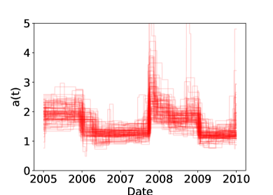
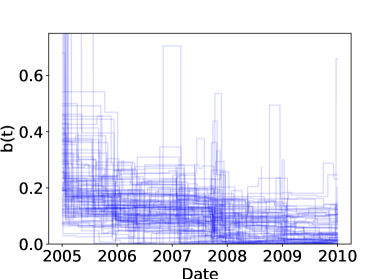
Figure S3: Posterior samples of the piecewise constant volatility functions $a(t)$ and $b(t)$ from 100 iterations of discontinuous Hamiltonian Monte Carlo.

S9 Error analysis of discontinuous Hamiltonian Monte Carlo integrator

Here we analyze the approximation error incurred by the integrator of Algorithm 2. We focus on the error in Hamiltonian, the amount by which the Hamiltonian fluctuates along a numerical solution, as it determines the acceptance probability of a proposal. An error incurred by one numerical integration step $(\bm{\theta}^{0},\bm{p}^{0})\to(\bm{\theta}^{1},\bm{p}^{1})$ of stepsize $\epsilon$ is known as a local error. Approximating the evolution $\{\bm{\theta}(0),\bm{p}(0)\}\to\{\bm{\theta}(\tau),\bm{p}(\tau)\}$ requires $L(\epsilon)=\lfloor\tau/\epsilon\rfloor$ numerical integration steps and the error incurred by the map $(\bm{\theta}^{0},\bm{p}^{0})\to(\bm{\theta}^{L},\bm{p}^{L})$ is known as a global error. We quantify the local error of Algorithm 2 in Section S9.1 and relate it to the global error in Section S9.2.

S9.1 Local error in Hamiltonian

In analyzing Algorithm 2, it is useful to break up the algorithm into three steps; the first (partial) update of continuous parameters, the update of discontinuous parameters, and the second update of continuous parameters. The notation $(\bm{\theta}_{I}^{\scalebox{0.7}{1/2}},\bm{p}_{I}^{\scalebox{0.7}{1/2}})$ will refer to the intermediate state after the first update of continuous parameters, namely $\bm{p}_{I}^{\scalebox{0.7}{1/2}}=\bm{p}_{I}^{0}-\frac{\epsilon}{2}\nabla_{\bm{\theta}_{I}}U(\bm{\theta}_{I}^{0},\bm{\theta}_{J}^{0})$ and $\bm{\theta}_{I}^{\scalebox{0.7}{1/2}}=\bm{\theta}_{I}^{0}+\frac{\epsilon}{2}\nabla_{\bm{p}_{I}}K(\bm{p}_{I}^{\scalebox{0.7}{1/2}},\bm{p}_{J}^{0})$ where $K(\bm{p})=\frac{1}{2}\,\bm{p}_{I}^{\intercal}\bm{M}_{I}^{-1}\bm{p}_{I}+\sum_{j\in J}m_{j}^{-1}|p_{j}|$ as before. The update $(\bm{\theta}_{I}^{0},\bm{p}_{I}^{0})\to(\bm{\theta}_{I}^{\scalebox{0.7}{1/2}},\bm{p}_{I}^{\scalebox{0.7}{1/2}})$ is followed by the update $(\bm{\theta}_{J}^{0},\bm{p}_{J}^{0})\to(\bm{\theta}_{J}^{1},\bm{p}_{J}^{1})$ of discontinuous parameters, which then is followed by another continuous parameter update $(\bm{\theta}_{I}^{\scalebox{0.7}{1/2}},\bm{p}_{I}^{\scalebox{0.7}{1/2}})\to(\bm{\theta}_{I}^{1},\bm{p}_{I}^{1})$. The exact solution is denoted by $\{\bm{\theta}(t),\bm{p}(t)\}$ with the initial condition $\{\bm{\theta}(0),\bm{p}(0)\}=(\bm{\theta}^{0},\bm{p}^{0})$.

The key result in this section is Corollary S9.2 below, which follows immediately from the following theorem:

Theorem S9.1.

The local error in Hamiltonian incurred by Algorithm 2 is given by

$$H(\bm{\theta}^{1},\bm{p}^{1})-H(\bm{\theta}^{0},\bm{p}^{0})=\frac{\epsilon^{2}}{8}\left\{\xi\left(\bm{\theta}_{I}^{\scalebox{0.7}{1/2}},\bm{\theta}_{J}^{1},\bm{p}_{I}^{\scalebox{0.7}{1/2}}\right)-\xi\left(\bm{\theta}_{I}^{\scalebox{0.7}{1/2}},\bm{\theta}_{J}^{0},\bm{p}_{I}^{\scalebox{0.7}{1/2}}\right)\right\}+O(\epsilon^{3}),$$ (S36)

where $\xi$ is defined in terms of the Hessians $\bm{\mathcal{I}}_{U}=\partial^{2}U/\partial\bm{\theta}_{I}^{2}$ and $\bm{\mathcal{I}}_{K}=\partial^{2}K/\partial\bm{p}_{I}^{2}$ with respect to continuous parameters as

$$\xi(\bm{\theta}_{I},\bm{\theta}_{J},\bm{p}_{I}) =\nabla_{\bm{\theta}_{I}}^{\intercal}U(\bm{\theta}_{I},\bm{\theta}_{J})\bm{\mathcal{I}}_{K}(\bm{p}_{I})\nabla_{\bm{\theta}_{I}}U(\bm{\theta}_{I},\bm{\theta}_{J})$$ (S37)

$$\hskip 30.00005pt-\nabla_{\bm{p}_{I}}^{\intercal}K(\bm{p}_{I})\bm{\mathcal{I}}_{U}(\bm{\theta}_{I},\bm{\theta}_{J})\nabla_{\bm{p}_{I}}K(\bm{p}_{I}).$$

As they are independent of $\bm{p}_{J}$, the derivatives of $K$ with respect to $\bm{p}_{I}$ are written simply as a function of $\bm{p}_{I}$ in the expression above.

Corollary S9.2.

The local error in Hamiltonian incurred by Algorithm 2 is $O(\epsilon^{3})$ when there is no discontinuity of $U$ along the line connecting $\bm{\theta}_{J}^{0}$ and $\bm{\theta}_{J}^{1}$. Otherwise, the local error is $O(\epsilon^{2})$.

Proof S9.3 (of Corollary S9.2).

When there is no discontinuity of $U$ along the line connecting $\bm{\theta}_{J}^{0}$ and $\bm{\theta}_{J}^{1}$, the Taylor expansion of $\xi$ as defined in (S37) with respect to $\bm{\theta}_{J}$ implies that

$$\xi\left(\bm{\theta}_{I}^{\scalebox{0.7}{1/2}},\bm{\theta}_{J}^{1},\bm{p}_{I}^{\scalebox{0.7}{1/2}}\right)-\xi\left(\bm{\theta}_{I}^{\scalebox{0.7}{1/2}},\bm{\theta}_{J}^{0},\bm{p}_{I}^{\scalebox{0.7}{1/2}}\right)=O(\|\bm{\theta}_{J}^{1}-\bm{\theta}_{J}^{0}\|)=O(\epsilon).$$ (S38)

Hence the leading order term of (S36) becomes $O(\epsilon^{3})$.

Proof S9.4 (of Theorem S9.1).

The update $(\bm{\theta}_{J}^{0},\bm{p}_{J}^{0})\to(\bm{\theta}_{J}^{1},\bm{p}_{J}^{1})$ is energy-preserving by the property of the coordinate-wise integrator, so we have

$$H(\bm{\theta}^{1},\bm{p}^{1})-H(\bm{\theta}^{0},\bm{p}^{0})$$ (S39)

$$\qquad=H(\bm{\theta}^{1},\bm{p}^{1})-H(\bm{\theta}_{I}^{\scalebox{0.7}{1/2}},\bm{\theta}_{J}^{1},\bm{p}_{I}^{\scalebox{0.7}{1/2}},\bm{p}_{J}^{1})+H(\bm{\theta}_{I}^{\scalebox{0.7}{1/2}},\bm{\theta}_{J}^{0},\bm{p}_{I}^{\scalebox{0.7}{1/2}},\bm{p}_{J}^{0})-H(\bm{\theta}^{0},\bm{p}^{0}).$$

Now let $(\bm{\theta}_{I}^{0}(t),\bm{p}_{I}^{0}(t))$ denote the solution of the differential equation

$$\frac{\textrm{d}\bm{\theta}_{I}}{\textrm{d}t}=\nabla_{\bm{p}_{I}}K(\bm{p}_{I},\bm{p}_{J}^{0}),\ \frac{\textrm{d}\bm{p}_{I}}{\textrm{d}t}=-\nabla_{\bm{\theta}_{I}}U(\bm{\theta}_{I},\bm{\theta}_{J}^{0})$$ (S40)

with the initial condition $\{\bm{\theta}_{I}^{0}(0),\bm{p}_{I}^{0}(0)\}=(\bm{\theta}_{I}^{0},\bm{p}_{I}^{0})$. Similarly, let $\{\bm{\theta}_{I}^{\scalebox{0.7}{1/2}}(t),\bm{p}_{I}^{\scalebox{0.7}{1/2}}(t)\}$ denote the solution of the differential equation

$$\frac{\textrm{d}\bm{\theta}_{I}}{\textrm{d}t}=\nabla_{\bm{p}_{I}}K(\bm{p}_{I},\bm{p}_{J}^{1}),\ \frac{\textrm{d}\bm{p}_{I}}{\textrm{d}t}=-\nabla_{\bm{\theta}_{I}}U(\bm{\theta}_{I},\bm{\theta}_{J}^{1})$$ (S41)

with the initial condition $\{\bm{\theta}_{I}^{\scalebox{0.7}{1/2}}(0),\bm{p}_{I}^{\scalebox{0.7}{1/2}}(0)\}=(\bm{\theta}_{I}^{\scalebox{0.7}{1/2}},\bm{p}_{I}^{\scalebox{0.7}{1/2}})$. By the energy-preserving property of exact Hamiltonian dynamics, (S39) becomes

$$H(\bm{\theta}^{1},\bm{p}^{1})-H(\bm{\theta}^{0},\bm{p}^{0})$$ (S42)

$$\qquad=H(\bm{\theta}^{1},\bm{p}^{1})-H\{\bm{\theta}_{I}^{\scalebox{0.7}{1/2}}(\epsilon/2),\bm{\theta}_{J}^{1},\bm{p}_{I}^{\scalebox{0.7}{1/2}}(\epsilon/2),\bm{p}_{J}^{1}\}$$

$$\hskip 40.00006pt+H(\bm{\theta}_{I}^{\scalebox{0.7}{1/2}},\bm{\theta}_{J}^{0},\bm{p}_{I}^{\scalebox{0.7}{1/2}},\bm{p}_{J}^{0})-H\{\bm{\theta}_{I}^{0}(\epsilon/2),\bm{\theta}_{J}^{0},\bm{p}^{0}(\epsilon/2),\bm{p}_{J}^{0}\}.$$

In essence, (S42) shows that the error in Hamiltonian comes only from the numerical approximation errors in solving the differential equations (S40) and (S41). Lemma S9.5 below quantifies such errors and its results can be related to the error in Hamiltonian by observing that

$$H(\bm{\theta}_{I}^{\scalebox{0.7}{1/2}},\bm{\theta}_{J}^{0},\bm{p}_{I}^{\scalebox{0.7}{1/2}},\bm{p}_{J}^{0})-H\{\bm{\theta}_{I}^{0}(\epsilon/2),\bm{\theta}_{J}^{0},\bm{p}_{I}^{0}(\epsilon/2),\bm{p}_{J}^{0}\}$$ (S43)

$$\qquad=U(\bm{\theta}_{I}^{\scalebox{0.7}{1/2}},\bm{\theta}_{J}^{0})-U\{\bm{\theta}_{I}^{0}(\epsilon/2),\bm{\theta}_{J}^{0}\}+K(\bm{p}_{I}^{\scalebox{0.7}{1/2}},\bm{p}_{J}^{0})-K\{\bm{p}_{I}^{0}(\epsilon/2),\bm{p}_{J}^{0}\}$$

$$\qquad=\nabla_{\bm{\theta}_{I}}^{\intercal}U(\bm{\theta}_{I}^{\scalebox{0.7}{1/2}},\bm{\theta}_{J}^{0})\big{\{}\bm{\theta}_{I}^{\scalebox{0.7}{1/2}}-\bm{\theta}_{I}^{0}(\epsilon/2)\big{\}}+\nabla_{\bm{p}_{I}}^{\intercal}K(\bm{p}_{I}^{\scalebox{0.7}{1/2}},\bm{p}_{J}^{0})\big{\{}\bm{p}_{I}^{\scalebox{0.7}{1/2}}-\bm{p}_{I}^{0}(\epsilon/2)\big{\}}$$

$$\hskip 50.00008pt+O\big{\{}\|\bm{\theta}_{I}^{\scalebox{0.7}{1/2}}-\bm{\theta}_{I}(\epsilon/2)\|^{2}\big{\}}+O\big{\{}\|\bm{p}_{I}^{\scalebox{0.7}{1/2}}-\bm{p}_{I}(\epsilon/2)\|^{2}\big{\}}.$$

Now applying (S48) of Lemma S9.5 with $\tilde{\epsilon}=\epsilon/2$, $(\bm{\theta}_{I},\bm{p}_{I})=(\bm{\theta}_{I}^{0},\bm{p}_{I}^{0})$, and $(\bm{\theta}_{I}^{*},\bm{p}_{I}^{*})=(\bm{\theta}_{I}^{\scalebox{0.7}{1/2}},\bm{p}_{I}^{\scalebox{0.7}{1/2}})$, we obtain

$$H(\bm{\theta}_{I}^{\scalebox{0.7}{1/2}},\bm{\theta}_{J}^{0},\bm{p}_{I}^{\scalebox{0.7}{1/2}},\bm{p}_{J}^{0})-H\{\bm{\theta}_{I}^{0}(\epsilon/2),\bm{\theta}_{J}^{0},\bm{p}_{I}^{0}(\epsilon/2),\bm{p}_{J}^{0}\}$$ (S44)

$$\qquad=-\frac{\epsilon^{2}}{8}\nabla_{\bm{\theta}_{I}}^{\intercal}U(\bm{\theta}_{I}^{\scalebox{0.7}{1/2}},\bm{\theta}_{J}^{0})\,\bm{\mathcal{I}}_{K}(\bm{p}_{I}^{\scalebox{0.7}{1/2}},\bm{p}_{J}^{0})\nabla_{\bm{\theta}_{I}}U(\bm{\theta}_{I}^{\scalebox{0.7}{1/2}},\bm{\theta}_{J}^{0})$$

$$\hskip 50.00008pt+\frac{\epsilon^{2}}{8}\nabla_{\bm{p}_{I}}^{\intercal}K(\bm{p}_{I}^{\scalebox{0.7}{1/2}},\bm{p}_{J}^{0})\bm{\mathcal{I}}_{U}(\bm{\theta}_{I}^{\scalebox{0.7}{1/2}},\bm{\theta}_{J}^{0})\nabla_{\bm{p}_{I}}K(\bm{p}_{I}^{\scalebox{0.7}{1/2}},\bm{p}_{J}^{0})+O(\epsilon^{3}).$$

In a similar manner, it follows from (S50) of Lemma S9.5 that

$$H(\bm{\theta}_{I}^{1},\bm{\theta}_{J}^{1},\bm{p}_{I}^{1},\bm{p}_{J}^{1})-H\{\bm{\theta}_{I}^{\scalebox{0.7}{1/2}}(\epsilon/2),\bm{\theta}_{J}^{1},\bm{p}_{I}^{\scalebox{0.7}{1/2}}(\epsilon/2),\bm{p}_{J}^{1}\}f$$ (S45)

$$\qquad=\frac{\epsilon^{2}}{8}\nabla_{\bm{\theta}_{I}}^{\intercal}U(\bm{\theta}_{I}^{1},\bm{\theta}_{J}^{1})\,\bm{\mathcal{I}}_{K}(\bm{p}_{I}^{\scalebox{0.7}{1/2}},\bm{p}_{J}^{1})\nabla_{\bm{\theta}_{I}}U(\bm{\theta}_{I}^{\scalebox{0.7}{1/2}},\bm{\theta}_{J}^{1})$$

$$\hskip 50.00008pt-\frac{\epsilon^{2}}{8}\nabla_{\bm{p}_{I}}^{\intercal}K(\bm{p}_{I}^{1},\bm{p}_{J}^{1})\bm{\mathcal{I}}_{U}(\bm{\theta}_{I}^{\scalebox{0.7}{1/2}},\bm{\theta}_{J}^{1})\nabla_{\bm{p}_{I}}K(\bm{p}_{I}^{\scalebox{0.7}{1/2}},\bm{p}_{J}^{1})+O(\epsilon^{3})$$

$$\qquad=\frac{\epsilon^{2}}{8}\nabla_{\bm{\theta}_{I}}^{\intercal}U(\bm{\theta}_{I}^{\scalebox{0.7}{1/2}},\bm{\theta}_{J}^{1})\,\bm{\mathcal{I}}_{K}(\bm{p}_{I}^{\scalebox{0.7}{1/2}},\bm{p}_{J}^{1})\nabla_{\bm{\theta}_{I}}U(\bm{\theta}_{I}^{\scalebox{0.7}{1/2}},\bm{\theta}_{J}^{1})$$

$$\hskip 50.00008pt-\frac{\epsilon^{2}}{8}\nabla_{\bm{p}_{I}}^{\intercal}K(\bm{p}_{I}^{\scalebox{0.7}{1/2}},\bm{p}_{J}^{1})\bm{\mathcal{I}}_{U}(\bm{\theta}_{I}^{\scalebox{0.7}{1/2}},\bm{\theta}_{J}^{1})\nabla_{\bm{p}_{I}}K(\bm{p}_{I}^{\scalebox{0.7}{1/2}},\bm{p}_{J}^{1})+O(\epsilon^{3}).$$

The result (S36) now follows by simply noting that the derivatives of $K$ with respect to $\bm{p}_{I}$ are independent of $\bm{p}_{J}$.

Lemma S9.5.

For $(\bm{\theta}_{J},\bm{p}_{J})$ fixed, let $\{\bm{\theta}_{I}(t),\bm{p}_{I}(t)\}$ denote the solution of the differential equation

$$\frac{\textrm{d}\bm{\theta}_{I}}{\textrm{d}t}=\nabla_{\bm{p}_{I}}K(\bm{p}_{I},\bm{p}_{J}),\ \frac{\textrm{d}\bm{p}_{I}}{\textrm{d}t}=-\nabla_{\bm{\theta}_{I}}U(\bm{\theta}_{I},\bm{\theta}_{J})$$ (S46)

with the initial condition $(\bm{\theta}_{I}(0),\bm{p}_{I}(0))=(\bm{\theta}_{I},\bm{p}_{I})$. The approximation error of the numerical scheme

$$\bm{\theta}_{I}^{*}=\bm{\theta}_{I}+\tilde{\epsilon}\nabla_{\bm{p}_{I}}K(\bm{p}_{I}^{*},\bm{p}_{J}),\ \bm{p}_{I}^{*}=\bm{p}_{I}-\tilde{\epsilon}\nabla_{\bm{\theta}_{I}}U(\bm{\theta}_{I},\bm{\theta}_{J})$$ (S47)

satisfies

$$\bm{\theta}_{I}^{*}-\bm{\theta}_{I}(\tilde{\epsilon})=-\frac{\tilde{\epsilon}^{2}}{2}\bm{\mathcal{I}}_{K}(\bm{p}_{I}^{*},\bm{p}_{J})\nabla_{\bm{\theta}_{I}}U(\bm{\theta}_{I}^{*},\bm{\theta}_{J})+O(\tilde{\epsilon}^{3})$$ (S48)

$$\bm{p}_{I}^{*}-\bm{p}_{I}(\tilde{\epsilon})=\frac{\tilde{\epsilon}^{2}}{2}\bm{\mathcal{I}}_{U}(\bm{\theta}_{I}^{*},\bm{\theta}_{J})\nabla_{\bm{p}_{I}}K(\bm{p}_{I}^{*},\bm{p}_{J})+O(\tilde{\epsilon}^{3})$$

where $\bm{\mathcal{I}}_{U}=\partial^{2}U/\partial\bm{\theta}_{I}^{2}$ and $\bm{\mathcal{I}}_{K}=\partial^{2}K/\partial\bm{p}_{I}^{2}$ are the Hessians of $U$ and $K$ with respect to $\bm{\theta}_{I}$ and $\bm{p}_{I}$. Similarly, the approximation error of the numerical scheme

$$\bm{\theta}_{I}^{*}=\bm{\theta}_{I}+\tilde{\epsilon}\nabla_{\bm{p}_{I}}K(\bm{p}_{I},\bm{p}_{J}),\ \bm{p}_{I}^{*}=\bm{p}_{I}-\tilde{\epsilon}\nabla_{\bm{\theta}_{I}}U(\bm{\theta}_{I}^{*},\bm{\theta}_{J})$$ (S49)

satisfies

$$\bm{\theta}_{I}^{*}-\bm{\theta}_{I}(\tilde{\epsilon})=\frac{\tilde{\epsilon}^{2}}{2}\bm{\mathcal{I}}_{K}(\bm{p}_{I},\bm{p}_{J})\nabla_{\bm{\theta}_{I}}U(\bm{\theta}_{I},\bm{\theta}_{J})+O(\tilde{\epsilon}^{3})$$ (S50)

$$\bm{p}_{I}^{*}-\bm{p}_{I}(\tilde{\epsilon})=-\frac{\tilde{\epsilon}^{2}}{2}\bm{\mathcal{I}}_{U}(\bm{\theta}_{I},\bm{\theta}_{J})\nabla_{\bm{p}_{I}}K(\bm{p}_{I},\bm{p}_{J})+O(\tilde{\epsilon}^{3}).$$

Proof S9.6.

The proofs of (S48) and (S50) are very similar, so we focus on the derivations of (S48). Taylor expansion of $\bm{\theta}_{I}(t)$ yields

$$\bm{\theta}_{I}(\tilde{\epsilon})-\bm{\theta}_{I} =\tilde{\epsilon}\frac{\textrm{d}\bm{\theta}}{\textrm{d}t}+\frac{\tilde{\epsilon}^{2}}{2}\frac{\textrm{d}^{2}\bm{\theta}}{\textrm{d}t^{2}}+O(\tilde{\epsilon}^{3})$$ (S51)

$$=\tilde{\epsilon}\nabla_{\bm{p}_{I}}K(\bm{p}_{I},\bm{p}_{J})-\frac{\tilde{\epsilon}^{2}}{2}\bm{\mathcal{I}}_{K}(\bm{p}_{I},\bm{p}_{J})\nabla_{\bm{\theta}_{I}}U(\bm{\theta}_{I},\bm{\theta}_{J})+O(\tilde{\epsilon}^{3}).$$

On the other hand, Taylor expansion of $\nabla_{\bm{p}_{I}}K(\bm{p}_{I}^{*},\bm{p}_{J})$ in the first variable yields

$$\bm{\theta}_{I}^{*}-\bm{\theta}_{I} =\tilde{\epsilon}\nabla_{\bm{p}_{I}}K(\bm{p}_{I},\bm{p}_{J})+\tilde{\epsilon}\,\bm{\mathcal{I}}_{K}(\bm{p}_{I},\bm{p}_{J})(\bm{p}_{I}^{*}-\bm{p}_{I})+\tilde{\epsilon}\,O(\|\bm{p}_{I}^{*}-\bm{p}_{I}\|^{2})$$ (S52)

$$=\tilde{\epsilon}\nabla_{\bm{p}_{I}}K(\bm{p}_{I},\bm{p}_{J})-\tilde{\epsilon}^{2}\bm{\mathcal{I}}_{K}(\bm{p}_{I},\bm{p}_{J})\nabla_{\bm{\theta}_{I}}U(\bm{\theta}_{I},\bm{\theta}_{J})+O(\tilde{\epsilon}^{3}).$$

Subtracting (S51) from (S52), we obtain

$$\bm{\theta}_{I}^{*}-\bm{\theta}_{I}(\tilde{\epsilon}) =-\frac{\tilde{\epsilon}^{2}}{2}\bm{\mathcal{I}}_{K}(\bm{p}_{I},\bm{p}_{J})\nabla_{\bm{\theta}_{I}}U(\bm{\theta}_{I},\bm{\theta}_{J})+O(\tilde{\epsilon}^{3})$$ (S53)

$$=-\frac{\tilde{\epsilon}^{2}}{2}\bm{\mathcal{I}}_{K}(\bm{p}_{I}^{*},\bm{p}_{J})\nabla_{\bm{\theta}_{I}}U(\bm{\theta}_{I}^{*},\bm{\theta}_{J})+O(\tilde{\epsilon}^{3}),$$

where the second equality again follows from a Taylor expansion applied to the leading order term. The error estimate for the momentum variable is similar; the Taylor expansion of $\bm{p}_{I}(t)$ gives

$$\bm{p}_{I}(\tilde{\epsilon})-\bm{p}_{I}=-\tilde{\epsilon}\nabla_{\bm{\theta}_{I}}U(\bm{\theta}_{I},\bm{\theta}_{J})-\frac{\tilde{\epsilon}^{2}}{2}\bm{\mathcal{I}}_{U}(\bm{\theta}_{I},\bm{\theta}_{J})\nabla_{\bm{p}_{I}}K(\bm{p}_{I},\bm{p}_{J})+O(\tilde{\epsilon}^{3}).$$ (S54)

Subtracting (S54) from (S47), we obtain

$$\begin{aligned} \bm{p}_{I}^{*}-\bm{p}_{I}(\tilde{\epsilon})&=\frac{\tilde{\epsilon}^{2}}{2}\bm{\mathcal{I}}_{U}(\bm{\theta}_{I},\bm{\theta}_{J})\nabla_{\bm{p}_{I}}K(\bm{p}_{I},\bm{p}_{J})+O(\tilde{\epsilon}^{3})\\ &=\frac{\tilde{\epsilon}^{2}}{2}\bm{\mathcal{I}}_{U}(\bm{\theta}_{I}^{*},\bm{\theta}_{J})\nabla_{\bm{p}_{I}}K(\bm{p}_{I}^{*},\bm{p}_{J})+O(\tilde{\epsilon}^{3}).\end{aligned}\hskip 20.00003pt\mbox{\QEDlogo}$$ (S55)

S9.2 Global error in Hamiltonian

Theorem S9.7 below establishes the global error in Hamiltonian to be $O(\epsilon^{2})$. For its proof, we recall that Algorithm 2 is designed under the assumption that the parameter space has a partition $\mathbb{R}^{|I|}\times\mathbb{R}^{|J|}=\cup_{k}\mathbb{R}^{|I|}\times\Omega_{k}$ such that $U(\bm{\theta})$ is smooth on $\mathbb{R}^{|I|}\times\Omega_{k}$ for each $k$. Below, in relating the local error to the global one, we make the dependence of a numerical solution on a stepsize $\epsilon$ explicit and denote the value of a numerical solution after $\ell$ steps by $(\bm{\theta}_{\epsilon}^{\ell},\bm{p}_{\epsilon}^{\ell})$.

Theorem S9.7.

Suppose that each $\Omega_{k}$ is rectangular so that its boundary consists of planes perpendicular to one of the coordinates of $\bm{\theta}_{J}$. Then the global error $H(\bm{\theta}_{\epsilon}^{L},\bm{p}_{\epsilon}^{L})-H(\bm{\theta}^{0},\bm{p}^{0})$, with $L=L(\epsilon)=\lfloor\tau/\epsilon\rfloor$, incurred by Algorithm 2 is of order $O\left(\epsilon^{2}D\right)$ where $D$ is the number of discontinuities in $U$ encountered along the trajectory $\{\bm{\theta}(t),0\leq t\leq\tau\}$.

The assumption stated in Theorem S9.7 is required for our proof of Theorem S9.9 and is satisfied whenever the discontinuous target $\pi$ is obtained by the embedding of discrete parameters described in Section 2.2. We however believe the order of the global error remains unchanged under more general conditions.

Proof S9.8.

The global error is given as a sum of the local errors:

$$H(\bm{\theta}_{\epsilon}^{L},\bm{p}_{\epsilon}^{L})-H(\bm{\theta}^{0},\bm{p}^{0})=\sum_{\ell=1}^{L}\left\{H(\bm{\theta}_{\epsilon}^{\ell},\bm{p}_{\epsilon}^{\ell})-H(\bm{\theta}_{\epsilon}^{\ell-1},\bm{p}_{\epsilon}^{\ell-1})\right\}$$ (S56)

Let $D(\epsilon)$ denote the size of the set $\mathcal{D}_{\epsilon}$ as defined below:

$$\mathcal{D}_{\epsilon} =\Big{\{}\ell\in\{1,\ldots,L\}:$$ (S57)

$$\hskip 30.00005pt\text{$\bm{\theta}_{\epsilon,J}^{\ell}$ and $\bm{\theta}_{\epsilon,J}^{\ell-1}$ belong to two separate regions of the partition $\Omega_{k}$'s}\Big{\}}$$

By the result of Corollary S9.2, we know that the local error is $O(\epsilon^{2})$ if $\ell\in\mathcal{D}_{\epsilon}$ and $O(\epsilon^{3})$ otherwise. Therefore, (S56) is a sum of $D(\epsilon)$ terms of $O(\epsilon^{2})$ errors and $L(\epsilon)-D(\epsilon)$ terms of $O(\epsilon^{3})$ errors, yielding the global error of $O\!\left\{D(\epsilon)\epsilon^{2}\right\}$. To complete the proof, it follows from Theorem S9.9 that $D(\epsilon)$ as $\epsilon\to 0$ converges to the number of discontinuities in $U$ encountered along the trajectory $\{\bm{\theta}(t),0\leq t\leq\tau\}$.

Theorem S9.9.

Under the assumption of Theorem S9.7, we have

$$\sup_{\ell=1,\ldots,L(\epsilon)}\big{\|}\{\bm{\theta}(\ell\epsilon),\bm{p}(\ell\epsilon)\}-(\bm{\theta}_{\epsilon}^{\ell},\bm{p}_{\epsilon}^{\ell})\big{\|}=O(\epsilon).$$ (S58)

Proof S9.10.

First note that the trajectory of Hamiltonian dynamics corresponding to the kinetic energy (17) can be partitioned into $\widetilde{D}$ segments $\{\bm{\theta}(t):t_{m}<t<t_{m+1}\}_{m}$ for $0=t_{0}<t_{1}<\ldots<t_{\widetilde{D}}=\tau$ so that on each segment $\textrm{d}\bm{\theta}_{J}/\textrm{d}t=\bm{m}_{J}^{-1}\odot\textrm{sign}(\bm{p}_{J})$ is constant.

The numerical solution approximates the exact solution $\bm{\theta}(t)\to\bm{\theta}(t+\ell\epsilon)$ up to an error of $O(\epsilon^{2})$ for any $\ell$ provided that $\bm{\theta}(t)$ and $\bm{\theta}(t+\ell\epsilon)$ belong to the same segment $\{\bm{\theta}(t):t_{m}<t<t_{m+1}\}$. This is for the following reason. For all sufficiently small $\epsilon$, the coordinate-wise updates of discontinuous parameters yield the exact solution to

$$\frac{\textrm{d}\bm{\theta}_{J}}{\textrm{d}t}=\bm{m}_{J}^{-1}\odot\textrm{sign}(\bm{p}_{J}),\quad\frac{\textrm{d}\bm{p}_{J}}{\textrm{d}t}=-\nabla_{\bm{\theta}_{J}}U(\bm{\theta}),\quad\frac{\textrm{d}\bm{\theta}_{\scalebox{1.0}{-}J}}{\textrm{d}t}=\frac{\textrm{d}\bm{p}_{\scalebox{1.0}{-}J}}{\textrm{d}t}=\bm{0}$$ (S59)

provided no sign change in $\bm{p}_{J}$ is encountered. In this case, Algorithm 2 coincides with a symmetric splitting of Hamilton’s equation in which the individual components are solved exactly and hence the numerical approximation of $\bm{\theta}(t)\to\bm{\theta}(t+\epsilon)$ locally agrees with the exact solution up to an error of $O(\epsilon^{3})$ (Leimkuhler & Reich, 2005).

Now consider the case when $\bm{\theta}(t)$ and $\bm{\theta}(t+\epsilon)$ do not belong to the same segment. In this case, the coordinate-wise integrator approximates the change in $\textrm{d}\bm{\theta}_{J}/\textrm{d}t$ through the momentum flip $p_{j}\to-p_{j}$ for an appropriate $j$ with $\theta_{j}$ held fixed. This may or may not be caused by a discontinuity in $U$ along the path $\{\bm{\theta}(s):t<s<t+\epsilon\}$. When there is no discontinuity, the approximation is always accurate up to an error of $O(\epsilon)$. When there is a discontinuity, our assumption on the boundaries of $\Omega_{k}$’s guarantees the numerical approximation error to be $O(\epsilon)$.

To summarize, we have shown that the total accumulated error is $O(\epsilon^{2})$ while the solution stays within the same segment $\{\bm{\theta}(t):t_{m}<t<t_{m+1}\}_{m}$ and then an additional error of $O(\epsilon)$ is incurred when crossing from one segment to another. Since the solution trajectory consists of $\widetilde{D}$ such segments, the total accumulated error is $O\{\widetilde{D}(\epsilon+\epsilon^{2})\}=O(\widetilde{D}\epsilon)$.

References

• Afshar & Domke (2015) Afshar, H. M. & Domke, J. (2015). Reflection, refraction, and Hamiltonian Monte Carlo. In Proceedings of the 28th International Conference on Neural Information Processing Systems.
• Ambrosio (2008) Ambrosio, L. (2008). Transport equation and cauchy problem for non-smooth vector fields. In Calculus of Variations and Nonlinear Partial Differential Equations. Springer, pp. 1–41.
• Andrieu & Thoms (2008) Andrieu, C. & Thoms, J. (2008). A tutorial on adaptive MCMC. Statistics and Computing 18, 343–373.
• Berger et al. (2012) Berger, J. O., Bernardo, J. M. & Sun, D. (2012). Objective priors for discrete parameter spaces. Journal of the American Statistical Association 107, 636–648.
• Beskos et al. (2013) Beskos, A., Pillai, N., Roberts, G., Sanz-Serna, J.-M. & Stuart, A. (2013). Optimal tuning of the hybrid Monte Carlo algorithm. Bernoulli 19, 1501–1534.
• Betancourt et al. (2014) Betancourt, M., Byrne, S. & Girolami, M. (2014). Optimizing the integrator step size for Hamiltonian Monte Carlo. arXiv:1411.6669 .
• Bierkens et al. (2017) Bierkens, J., Bouchard-Côté, A., Doucet, A., Duncan, A. B., Fearnhead, P., Roberts, G. & Vollmer, S. J. (2017). Piecewise deterministic Markov processes for scalable Monte Carlo on restricted domains. arXiv:1701.04244 .
• Bierkens et al. (2016) Bierkens, J., Fearnhead, P. & Roberts, G. (2016). The zig-zag process and super-efficient sampling for Bayesian analysis of big data. arXiv:1607.03188 .
• Bissiri et al. (2016) Bissiri, P. G., Holmes, C. C. & Walker, S. G. (2016). A general framework for updating belief distributions. Journal of the Royal Statistical Society: Series B (Statistical Methodology) 78, 1103–1130.
• Bou-Rabee et al. (2017) Bou-Rabee, N., Sanz-Serna, J. M. et al. (2017). Randomized Hamiltonian Monte Carlo. The Annals of Applied Probability 27, 2159–2194.
• Carpenter et al. (2015) Carpenter, B., Hoffman, M. D., Brubaker, M., Lee, D., Li, P. & Betancourt, M. (2015). The Stan math library: Reverse-mode automatic differentiation in C++. arXiv:1509.07164 .
• Carvalho et al. (2010) Carvalho, C. M., Polson, N. G. & Scott, J. G. (2010). The horseshoe estimator for sparse signals. Biometrika 97, 465–480.
• Chib (1998) Chib, S. (1998). Estimation and comparison of multiple change-point models. Journal of Econometrics 86, 221–241.
• Chopin & Ridgway (2017) Chopin, N. & Ridgway, J. (2017). Leave Pima indians alone: binary regression as a benchmark for Bayesian computation. Statistical Science 32, 64–87.
• Dinh et al. (2017) Dinh, V., Bilge, A., Zhang, C. & Matsen IV, F. A. (2017). Probabilistic path Hamiltonian Monte Carlo. In Proceedings of the 34th International Conference on Machine Learning, vol. 70.
• Duane et al. (1987) Duane, S., Kennedy, A. D., Pendleton, B. J. & Roweth, D. (1987). Hybrid Monte Carlo. Physics Letters B 195, 216–222.
• Durmus et al. (2017) Durmus, A., Moulines, E. & Saksman, E. (2017). On the convergence of Hamiltonian Monte Carlo. arXiv:1705.00166 .
• Fang et al. (2014) Fang, Y., Sanz-Serna, J. M. & Skeel, R. D. (2014). Compressible generalized hybrid Monte Carlo. The Journal of Chemical Physics 140, 174108.
• Fearnhead et al. (2016) Fearnhead, P., Bierkens, J., Pollock, M. & Roberts, G. O. (2016). Piecewise deterministic Markov processes for continuous-time Monte Carlo. arXiv:1611.07873 .
• Fryzlewicz & Subba Rao (2014) Fryzlewicz, P. & Subba Rao, S. (2014). Multiple-change-point detection for auto-regressive conditional heteroscedastic processes. Journal of the Royal Statistical Society: Series B (Statistical Methodology) 76, 903–924.
• Gelman (2006) Gelman, A. (2006). Prior distributions for variance parameters in hierarchical models. Bayesian Analysis 1, 515–534.
• Gelman et al. (2013) Gelman, A., Carlin, J. B., Stern, H. S., Dunson, D. B., Vehtari, A. & Rubin, D. B. (2013). Bayesian Data Analysis. CRC Press.
• Gelman et al. (2015) Gelman, A., Lee, D. & Guo, J. (2015). Stan: a probabilistic programming language for Bayesian inference and optimization. Journal of Educational and Behavior Science 40, 530–543.
• Gelman et al. (1996) Gelman, A., Roberts, G. O. & Gilks, W. R. (1996). Efficient Metropolis jumping rules. Bayesian Statistics 5, 599–607.
• Geyer (2011) Geyer, C. (2011). Introduction to Markov chain Monte Carlo. In Handbook of Markov Chain Monte Carlo. CRC Press, pp. 3–48.
• Girolami & Calderhead (2011) Girolami, M. & Calderhead, B. (2011). Riemann manifold Langevin and Hamiltonian Monte Carlo methods. Journal of the Royal Statistical Society: Series B (Statistical Methodology) 73, 123–214.
• Gram-Hansen et al. (2018) Gram-Hansen, B., Zhou, Y., Kohn, T., Yang, H. & Wood, F. (2018). Discontinuous Hamiltonian Monte Carlo for probabilistic programs. arXiv:1804.03523 .
• Griewank & Walther (2008) Griewank, A. & Walther, A. (2008). Evaluating derivatives: principles and techniques of algorithmic differentiation. Society for Industrial and Applied Mathematics.
• Gustafson (1998) Gustafson, P. (1998). A guided walk Metropolis algorithm. Statistics and Computing 8, 357–364.
• Haario et al. (2001) Haario, H., Saksman, E. & Tamminen, J. (2001). An adaptive Metropolis algorithm. Bernoulli , 223–242.
• Haario et al. (2005) Haario, H., Saksman, E. & Tamminen, J. (2005). Componentwise adaptation for high dimensional MCMC. Computational Statistics 20, 265–273.
• Hairer et al. (2006) Hairer, E., Lubich, C. & Wanner, G. (2006). Geometric Numerical Integration. Structure-Preserving Algorithms for Ordinary Differential Equations. Springer-Verlag.
• Hirsch & Smale (1974) Hirsch, M. & Smale, S. (1974). Differential Equations, Dynamical Systems, and Linear Algebra. Academic Press.
• Hoffman & Gelman (2014) Hoffman, M. D. & Gelman, A. (2014). The no-U-turn sampler: adaptively setting path lengths in Hamiltonian Monte Carlo. Journal of Machine Learning Research 15, 1593–1623.
• Johnson et al. (2013) Johnson, A. A., Jones, G. L. & Neath, R. C. (2013). Component-wise Markov chain Monte Carlo: Uniform and geometric ergodicity under mixing and composition. Statistical Science , 360–375.
• Jolly (1965) Jolly, G. M. (1965). Explicit estimates from capture-recapture data with both death and immigration-stochastic model. Biometrika 52, 225–247.
• Kruschke (2014) Kruschke, J. (2014). Doing Bayesian Data Analysis, Second Edition: A Tutorial with R, JAGS, and Stan. Academic Press.
• Leimkuhler & Reich (2005) Leimkuhler, B. & Reich, S. (2005). Simulating Hamiltonian Dynamics. Cambridge University Press.
• Livingstone et al. (2016) Livingstone, S., Betancourt, M., Byrne, S. & Girolami, M. (2016). On the geometric ergodicity of Hamiltonian Monte Carlo. arXiv:1601.08057 .
• Livingstone et al. (2019) Livingstone, S., Faulkner, M. F. & Roberts, G. O. (2019). Kinetic energy choice in Hamiltonian/hybrid Monte Carlo. Biometrika 106, 303–319.
• Lu et al. (2017) Lu, X., Perrone, V., Hasenclever, L., Teh, Y. W. & Vollmer, S. (2017). Relativistic Monte Carlo. In Proceedings of the 20th International Conference on Artificial Intelligence and Statistics, vol. 54.
• Lunn et al. (2009) Lunn, D., Spiegelhalter, D., Thomas, A. & Best, N. (2009). The BUGS project: Evolution, critique and future directions. Statistics in Medicine 28, 3049–3067.
• McLachlan & Quispel (2002) McLachlan, R. I. & Quispel, G. R. W. (2002). Splitting methods. Acta Numerica 11, 341–434.
• Metropolis et al. (1953) Metropolis, N., Rosenbluth, A. W., Rosenbluth, M. N., Teller, A. H. & Teller, E. (1953). Equation of state calculations by fast computing machines. The Journal of Chemical Physics 21, 1087–1092.
• Monnahan et al. (2017) Monnahan, C. C., Thorson, J. T. & Branch, T. A. (2017). Faster estimation of Bayesian models in ecology using Hamiltonian Monte Carlo. Methods in Ecology and Evolution 8, 339––348.
• Nakajima & West (2013) Nakajima, J. & West, M. (2013). Bayesian analysis of latent threshold dynamic models. Journal of Business & Economic Statistics 31, 151–164.
• Neal (1996) Neal, R. M. (1996). Bayesian Learning for Neural Networks. Springer-Verlag.
• Neal (2010) Neal, R. M. (2010). MCMC using Hamiltonian Dynamics. In Handbook of Markov chain Monte Carlo. CRC Press.
• Neelon & Dunson (2004) Neelon, B. & Dunson, D. B. (2004). Bayesian isotonic regression and trend analysis. Biometrics 60, 398–406.
• Nishimura & Dunson (2015) Nishimura, A. & Dunson, D. (2015). Recycling intermediate steps to improve Hamiltonian Monte Carlo. arXiv:1511.06925 .
• Pakman & Paninski (2013) Pakman, A. & Paninski, L. (2013). Auxiliary-variable exact Hamiltonian Monte Carlo samplers for binary distributions. In Proceedings of the 26th International Conference on Neural Information Processing Systems.
• Roberts et al. (1997) Roberts, G. O., Gelman, A. & Gilks, W. R. (1997). Weak convergence and optimal scaling of random walk Metropolis algorithms. The Annals of Applied Probability 7, 110–120.
• Roberts & Rosenthal (2009) Roberts, G. O. & Rosenthal, J. S. (2009). Examples of adaptive MCMC. Journal of Computational and Graphical Statistics 18, 349–367.
• Salvatier et al. (2016) Salvatier, J., Wiecki, T. V. & Fonnesbeck, C. (2016). Probabilistic programming in Python using PyMC3. PeerJ Computer Science 2, e55.
• Schwarz & Arnason (1996) Schwarz, C. J. & Arnason, A. N. (1996). A general methodology for the analysis of capture-recapture experiments in open populations. Biometrics , 860–873.
• Schwarz & Seber (1999) Schwarz, C. J. & Seber, G. A. F. (1999). Estimating animal abundance: Review III. Statistical Science 14, 427–456.
• Seber (1982) Seber, G. A. F. (1982). The Estimation of Animal Abundance. Griffin London.
• Stan Development Team (2016) Stan Development Team (2016). Stan Modeling Language Users Guide and Reference Manual, Version 2.14.0.
• Stewart (2000) Stewart, D. E. (2000). Rigid-body dynamics with friction and impact. SIAM Review 42, 3–39.
• Thawornwattana et al. (2018) Thawornwattana, Y., Dalquen, D., Yang, Z. et al. (2018). Designing simple and efficient markov chain monte carlo proposal kernels. Bayesian Analysis 13, 1033–1059.
• Wagner et al. (2002) Wagner, A. K., Soumerai, S. B., Zhang, F. & Ross-Degnan, D. (2002). Segmented regression analysis of interrupted time series studies in medication use research. Journal of Clinical Pharmacy and Therapeutics 27, 299–309.
• Zhang et al. (2012) Zhang, Y., Sutton, C., Storkey, A. & Ghahramani, Z. (2012). Continuous relaxations for discrete Hamiltonian Monte Carlo. In Proceedings of the 25th International Conference on Neural Information Processing Systems.
• Zhang et al. (2016) Zhang, Y., Wang, X., Chen, C., Henao, R., Fan, K. & Carin, L. (2016). Towards unifying Hamiltonian Monte Carlo and slice sampling. In Advances in Neural Information Processing Systems.