Vehicle Traffic Driven Camera Placement for Better Metropolis Security Surveillance

Abstract

Security surveillance is one of the most important issues in smart cities, especially in an era of terrorism. Deploying a number of (video) cameras is a common surveillance approach. Given the never-ending power offered by vehicles to metropolises, exploiting vehicle traffic to design camera placement strategies could potentially facilitate security surveillance. This article constitutes the first effort toward building the linkage between vehicle traffic and security surveillance, which is a critical problem for smart cities. We expect our study could influence the decision making of surveillance camera placement, and foster more research of principled ways of security surveillance beneficial to our physical-world life. Code has been made publicly available.

I Introduction

Security surveillance is one of the most important issues in smart cities. Due to the continuous growth of cities in size and complexity, keeping cities safe becomes critical to attracting skilled people and investments necessary for economic growth and development. Compounded by terrorism, cities, especially metropolises, have to carefully conduct security surveillance.

To fight against the adversary, deploying a number of (video) cameras is a common surveillance approach, which has gained prominence in policy proposals on combating terrorism [1]. At first glance, camera placement is a trivial task that could be achieved by simply purchasing a huge number of cameras. However, subject to the economic budget, cameras cannot be placed unlimitedly. Additionally, as the camera resolution increases, the network bandwidth (and the storage and processing overhead) needed for real-time transmission of the recorded videos to the data center is considerably large. For example, the latest generation of IP cameras require up to 10 Mbps bandwidth per camera [2]. Theses constraints will become more significant as cities grow in size and complexity.

Exploiting vehicle traffic from cyber transportation space to strategically place cameras could potentially facilitate physical-world security surveillance. For example, criminals and terrorists may drive vehicles before and after security events occur; vehicles have become terrorists’ favorable weapons, such as the 2017 Westminster attack [3]. Thus, monitoring vehicles has great potential in collecting security event evidence.

As a straightforward strategy, one may place cameras in busy (e.g., more traffic) regions, where the adversary tends to commit crimes or large-scale threatening terrorism activities. However, this strategy may fail to cover vehicles that never enter busy regions. Intuitively, a good strategy should allow distinct vehicles visible to cameras as many as possible, and make each vehicle exposed to cameras frequently. The former requirement is very important because the invisibility of a vehicle to cameras means the lack of surveillance. The latter requirement encourages more information to be collected for each vehicle, making it more likely to recognize the trajectory of a vehicle.

After placing the camera infrastructure, we also expect the placed cameras to be of high resolution for high-quality video data. However, as the number of placed cameras grows, the overhead of handling the data (e.g., transmission, storage and processing) may become intractable. That is, despite the large population of placed cameras, the number of cameras that could be of high resolution simultaneously is limited. Determining which cameras should be of high resolution is a non-trivial task. If a fixed set of cameras are configured as high resolution, the adversary may evade these cameras (when committing crimes), thereby eliminating high-quality crime evidence.

Focusing on these problems, this article investigates vehicle traffic driven security camera infrastructure placement, and formulates it as a group of submodular set function optimization problems, which could be gracefully solved by the greedy algorithm with theoretical lower bounds. We propose five different placement strategies that differ in designing goals. Also, we design a randomized camera resolution upgrading framework based on game theory, with the purpose of breaching the practical overhead barrier of handing video data. Using the carefully designed randomized strategy, we can deter the sophisticated adversary with maximal utility.

Our work constitutes the first effort toward building the linkage between vehicle traffic and security surveillance, which is a critical problem for smart cities. We expect our study could influence the decision making of surveillance camera placement, and foster more research efforts towards principled ways of security surveillance beneficial to our physical-world life.

II Vehicle Traffic Driven Placement Strategies for Building Surveillance Infrastructure

II-A Problem Description

Let $V$ be the set of vehicles under surveillance and $v\in V$ be a vehicle. Suppose $v$ is equipped with a position sensor. The coordinates include latitude and longitude. Specifically, the data from the sensor comprises the following fields: (vehicle ID, time, latitude, longitude), where the vehicle ID uniquely identifies a vehicle.

The metropolis is characterized as a rectangle uniquely identified by its maximum latitude, minimum latitude, maximum longitude, and minimum longitude. The rectangle is divided into small blocks with a size of $l\times l$ (e.g., $50m\times 50m$), resulting in a set of blocks denoted by $\Omega$. The advantages of dividing the map into blocks are two-fold, namely, map-independent (applicable for all metropolises) and exactly covering the entire map (unlike circulars).

Our goal is to find a subset of blocks $C\subseteq\Omega$ to place (super) cameras, so that the security surveillance utility could be maximized. The cardinality of $C$ is the number of blocks that we select to place cameras. Let $N$ denote the maximum number of blocks where we can afford to place cameras. Obviously, we have $|C|\leq N$. Note that only a block with GPS records can be selected for camera placement, thereby containing at least one road.

II-B Placement Strategies

For all strategies, we denote the objective function by $F(C)$.

II-B1 S1—Maximum Unique Vehicles

This strategy selects a subset $C\subseteq\Omega$ so that the number of unique vehicles crossing (at least one) blocks in $C$ is maximized, formally expressed as

$$\operatorname*{argmax}_{C}F(C)=\sum_{v\in V}I_{v}(C)$$ (1)

where $I_{v}(C)$ equals one if $v$ has crossed at least one block in $C$; otherwise $I_{v}(C)$ equals 0. Such a strategy maximizes the visibility space (i.e., the total number of unique vehicles) of security surveillance.

II-B2 S2—Maximum Vehicle Traffic

This strategy differs from S1 in that it maximizes the amount of vehicle traffic (rather than unique vehicles) crossing blocks in $C$. Similarly, it is

$$\operatorname*{argmax}_{C}F(C)=\sum_{v\in V}T_{v}(C)$$ (2)

where $T_{v}(C)$ denotes the amount of traffic of blocks in $C$ contributed by $v$, and could be measured by the total time when $v$ stays inside $C$. $T_{v}(C)$ can be calculated by $\sum_{c\in C}T_{v}(c)$, where $T_{v}(c)$ denotes the total time when $v$ stays in $c$, depending on the times when $v$ enters and leaves $c$. S2 maximizes the total visible time to cameras of all vehicles (i.e., summing up the time each vehicle under surveillance).

II-B3 S3—Minimum Mean OITR (Out-Camera to In-Camera Time Ratio)

This strategy minimizes the mean OITR across all vehicles. The OITR of a vehicle represents the proportion of time when a vehicle is outside the visible scope of cameras. Intuitively, smaller mean OITR across all vehicles indicates better security surveillance. S3 is equivalent to the maximization problem:

$$\operatorname*{argmax}_{C}F(C)=\Phi-\sum_{v\in V}\left(\frac{S}{T_{v}(C)+1}-1\right)/{|V|}$$ (3)

where $S$ is the measurement time. S3 does not take the uniqueness of cameras into consideration. Therefore, it encourages more unique vehicles visible to (whichever) cameras, and meanwhile each vehicle visible to cameras as long as possible. Note that $T_{v}(C)$ is increased by one to avoid $S$ being divided by zero, and $\Phi$ is a constant derived from $F(\emptyset)=0$ so that we have $F(C)\geq 0$. The same operation exists for S4 and S5.

II-B4 S4—Minimum Mean ACIs (Average Camera-Hit Intervals)

We define the ACIs to represent the average time interval to hit a 　 camera for a vehicle. Formally, we minimize the mean ACIs across all vehicles, and $S4$ is equivalent to:

$$\operatorname*{argmax}_{C}F(C)=\Phi-\sum_{v\in V}\frac{S}{H_{v}(C)+1}/{|V|}$$ (4)

where $H_{v}(C)$ denotes the number of times that vehicle $v$ hits (whichever) cameras along its trajectory during the measurement time $S$. S4 encourages more unique vehicles visible to (whichever) cameras, and meanwhile each vehicle to hit cameras more frequently.

II-B5 S5—Minimum Mean AUIs (Average Unique-Camera-Hit Intervals)

We further adapt $S4$ by considering the uniqueness of cameras that a vehicle hits. Accordingly, we define the AUIs to represent the average time interval to hit a new camera for a vehicle. Similar to S4, we minimize the mean AUIs across all vehicles, and S5 is defined as:

$$\operatorname*{argmax}_{C}F(C)=\Phi-\sum_{v\in V}\frac{S}{U_{v}(C)+1}/{|V|}$$ (5)

where $U_{v}(C)$ denotes the number of unique cameras that vehicle $v$ hits during the measurement time $S$. $U_{v}(C)$ is calculated as the number of unique blocks in $C$ that $v$ crosses. S5 encourages more unique vehicles visible to (whichever) cameras, and meanwhile each vehicle to hit more new cameras.

II-C Solving Optimal Placement Strategies

All the above strategies are formulated as maximization problems under the constraint $|C|\leq N$. To find a subset of blocks $C\subseteq\Omega$ to place cameras so that $F(C)$ can be maximized, we need to solve these maximization problems, which are NP-hard.

Each strategy differs in the objective function $F(C)$. However, this does not necessarily mean that we have to solve these strategies in five different manners. Instead, all these maximization problems could be gracefully solved with a greedy algorithm (GA) because of their non-increasing monotony and submodularity [4, 5]. The non-increasing monotony means that, for any two sets $C_{1},C_{2}\subseteq\Omega$ and $C_{1}\subseteq C_{2}$, we have $F(C_{1})\leq F(C_{2})$. Apparently, the functions defined in S1$\sim$S5 are non-decreasing.

The submodularity means that a non-decreasing set function has the property of diminishing returns when a single element $c$ is added to an input set $C$, as compared to $c$ is added to an input set that is a subset of $C$. Specifically, for a non-decreasing function, such as $F(C)$ defined in S1$\sim$S5, given every two sets $C_{1},C_{2}\subseteq\Omega$ and $C_{1}\subseteq C_{2}$, and a new block $c\in\Omega\setminus C_{2}$, the submodular property is equivalent to $F(C_{1}\cup\{c\})-F(C_{1})\geq F(C_{2}\cup\{c\})-F(C_{2})$. This means smaller sets have more function value increment when they are added with a new block. It is easy to prove the the submodularity for S1 and S2. The proof of the submodularity for S3$\sim$S5 is included in the appendix. Interested readers are referred to [5] for a comprehensive survey of submodularity.

According to [4], submodularity allows us to derive a solution lower bounded by $1-1/e\approx 63\%$ of the optimal solution. GA runs for at most $N$ rounds to obtain a set $C$ of size $|C|\leq N$. In each round, it selects a new block $c\in\Omega\setminus C$ maximizing the reward gain, $\delta_{c}(C)=F(C\cup{c})-F(C)$, and inserts $c$ into $C$. This process repeats until $|C|=N$ or $\delta_{c}(C)=0$.

III Randomizing Camera Resolution Upgrading for High-quality Surveillance

As the number of the affordable cameras grows, the overhead of handling the videos (e.g., transmission, storage and processing) may be impossible to satisfy, especially when high-resolution video is desired for high-quality crime evidence [6]. In other words, only a limited number of cameras could be of high resolution simultaneously.

Determining which cameras should be of high resolution is non-trivial. If a fixed set of cameras are configured as high resolution, the adversary may evade them deliberately (when committing crimes), thereby eliminating high-quality crime evidence. Therefore, we propose to randomly choose a set of placed cameras and upgrade their resolution, with an attempt to deter the adversary by making him feel that any camera might be of high resolution.

III-A A Game-theoretic Formulation

Since different blocks differ in their priorities to be monitored, or to be the target blocks where criminal activities are committed, we take into account the importance of different blocks when designing the randomized strategy. Meanwhile, the adversary aims to evade the surveillance of high-resolution cameras, while the defender (e.g., police) tries to observe the adversary.

To describe such confrontation, we leverage the Stackelberg security game (SSG) to design the strategy [7]. SSG is well-suited to adversarial reasoning for security resource allocation problems and has been adopted in many applications, such as US Federal Air Marshal Service [8].

A standard SSG has two players, a leader and a follower. Each player has its own set of pure strategies to select. The leader and the follower act sequentially as follows.

Step 1. The leader (i.e., defender) commits to a mixed strategy. The mixed strategy allows the leader to play a probability distribution over pure strategies, maximizing the leader’s utility.

Step 2. The follower (i.e., adversary), as a response, selects a pure strategy that optimizes his utility after inspecting and learning the mixed strategy chosen by the leader.

We consider a threat model wherein the adversary is sophisticated. Specifically, the adversary can inspect and learn the monitor’s mixed strategy (i.e., the probability distribution), and select the pure strategy that maximizes his utility, i.e., a best response adversary.

On the other hand, the defender is forward-looking. That is, she takes into account the adversary’s threat model when designing strategies, thereby making her strategy robust against the sophisticated adversary.

Although the adversary can learn the defender’s mixed strategy, he cannot predict which specific pure strategy the defender would adopt at the time of his scheduled criminal activities.

III-B Player Strategies

A pure strategy of the defender is a set of cameras whose resolution can be upgraded simultaneously. Our aim is to deter the adversary by randomly upgrading the resolution of the placed cameras, and thus the adversary committing crimes in blocks without cameras are not considered. Therefore, a pure strategy of the adversary is a set of blocks with placed cameras.

III-C Utility Functions

Consider that the adversary commits crimes in the $i$th block $c_{i}$. If $c_{i}$ is covered by the defender’s pure strategy, the defender receives reward $R_{i}^{d}$. Otherwise, the defender receives penalty $P_{i}^{d}$. Similarly, the adversary receives penalty $P_{i}^{a}$ in the former case, and reward $R_{i}^{a}$ in the latter case.

The reward that the defender monitors a specific block can be assigned according to the importance of the block, such as the amount of vehicle traffic, the number of unique vehicles, and historical crime activity severity, and so forth. The penalty that the adversary selects a block can be measured in the same way.

Let $\Gamma_{j}$ denote the $j$th defender pure strategy, and $A_{ij}$ denotes the coverage indicator of $\Gamma_{j}$ on $c_{i}$, where $A_{ij}=1$ for $c_{i}\in\Gamma_{j}$, and $A_{ij}=0$ for $c_{i}\notin\Gamma_{j}$. Let $J$ be the number of defender pure strategies. The number of adversary pure strategies is $N$, the (maximum) number of blocks where cameras are placed. We denote the probability of the defender choosing pure strategy $\Gamma_{j}$ by $a_{j}$, and we have

$$\sum_{j=1}^{J}a_{j}=1$$ (6)

The marginal probability $x_{i}$ for the defender to upgrade $c_{i}$ (i.e., upgrade the resolution of the camera in $c_{i}$) can be calculated by

$$x_{i}=\sum_{j=1}^{J}a_{j}A_{ij},i=1,2\ldots,N$$ (7)

We denote $(a_{1},a_{2},\ldots,a_{J})$ by $\mathbf{a}$, and $(x_{1},x_{2},\ldots,x_{N})$ by $\mathbf{x}$, where $\mathbf{x}$ is determined by $\mathbf{a}$.

The defender’s expected utility on upgrading $c_{i}$ can be expressed as

$$\begin{split}U_{i}^{d}(x_{i})&=x_{i}R_{i}^{d}+(1-x_{i})P_{i}^{d}\end{split}$$ (8)

and the adversary’s expected utility on committing crimes in $c_{i}$ is:

$$\begin{split}U_{i}^{a}(x_{i})&=x_{i}P_{i}^{a}+(1-x_{i})R_{i}^{a}\end{split}$$ (9)

III-D Mixed Strategy against A Best Response Adversary

We formally define the objective function with constraints to maximize the defender’s utility against a best response adversary. Let us first consider a sophisticated adversary who takes the best response, i.e., selecting the block to commit crimes so to maximize his utility. In this case, the probability that the adversary selects $c_{i}$ equals

$$B_{i}=\begin{cases}1&U_{i}^{a}(x_{i})\geq U_{j}^{a}(x_{j}),\forall j=1,\ldots,J\\ 0&\text{otherwise}\end{cases}$$ (10)

This means that the adversary knows the marginal probability $x_{i}$ for the defender to upgrade $c_{i}$, and he selects the target with maximal expected utility. Consequently, the utility functions of the adversary and the defender can be expressed as

$$U^{a}=\sum_{i=1}^{N}B_{i}U_{i}^{a}(x_{i})$$ (11)

$$U^{d}=\sum_{i=1}^{N}B_{i}U_{i}^{d}(x_{i})$$ (12)

Simultaneously, the defender selects an optimal mixed (i.e., randomized) strategy in consideration of the sophisticated adversary’s best response. The defender maximizes her utility $U^{d}$ as

$$\max_{\mathbf{a}}\sum_{i=1}^{N}B_{i}U_{i}^{d}(x_{i})$$ (13)

Substituting (8), we rewrite (13) as

$$\max_{\mathbf{a}}\sum_{i=1}^{N}B_{i}\left(x_{i}R_{i}^{d}+(1-x_{i})P_{i}^{d}\right)$$ (14)

To calculate the defender’s optimal strategy, the following problem P1 needs to be solved.

$$\textbf{P1:}\!\left\{\begin{split}&\max_{\mathbf{a}}\sum_{i=1}^{N}B_{i}\left(x_{i}R_{i}^{d}+(1-x_{i})P_{i}^{d}\right)\\ &\text{subject to }\hskip 42.67912ptx_{i}=\sum_{j=1}^{J}a_{j}A_{ij}\text{, }\forall i\\ &\hskip 85.35826pt\sum_{j=1}^{J}a_{j}=1\\ &\hskip 85.35826pt0\leq a_{j}\leq 1\text{, }\forall j\end{split}\right.$$ (15)

Problem P1 cannot be directly solved since $B_{i}$ defined in (10) contains an underlying “if-then” logical relationship. Instead, after removing the “if-then” logical relationship, P1 can be readily solved by the branch-and-cut algorithm [9].

The defender finally adopts the mixed strategy below.

$$\small\boxed{\begin{aligned} &\text{Mixed Strategy: }\text{play }\Gamma_{j}\text{with probability }a_{j}\hskip 28.45274pt\\ &\hskip 19.91692pt\text{where }a_{j}\in\mathbf{a}\text{ is the solution of problem P1}\\ &\hskip 19.91692ptj=1,2,\ldots,J\end{aligned}}$$

IV Experimental Evaluation

IV-A Dataset Description

The data contains one-week GPS trajectories of 10,357 taxis in Beijing, with more than 15 million position records and 9 million kilometers total distance of the trajectories [10]. We remove the outliers along the GPS trajectories of a vehicle, including points indicating an impossible speed, and points that significantly deviate the moving average. Finally, we identify 0.28% of all the GPS points as outliers.

We then divide Beijing into a set of blocks $\Omega$ with a size of $50m\times 50m$, yielding the total number of such blocks $|\Omega|=14,473,089$. We can place cameras in blocks where vehicles arrive. There are 438,674 such blocks, denoted as $R\subset\Omega$.

IV-B Performance of Camera Placement Strategies

IV-B1 Metrics

Larger values of these metrics indicate better security surveillance.

• UCR (Unique Vehicle Coverage Ratio). The ratio of observed unique vehicles to all vehicles, calculated by $\sum_{v\in V}I_{v}(C)/\sum_{v\in V}I_{v}(R)$.

• VCR (Vehicle Traffic Coverage Ratio). The ratio of traffic observed by all cameras to the total amount of traffic, which equals $\sum_{v\in V}T_{v}(C)/\sum_{v\in V}T_{v}(R)$.

• VIT (Vehicle In-Camera Time). The total amount of time when a vehicle $v$ is under surveillance, i.e., $T_{v}(C)$

• VCH (Vehicle Camera-Hits). The number of times that $v$ hits cameras along its trajectory, calculated as $\sum_{c\in C}I^{\prime}_{v}(\{c\})$, where $I^{\prime}_{v}(\{c\})$ is the number of times $v$ hits block $c\in C$.

• VUH (Vehicle Unique-Camera-Hits). The number of unique cameras $v$ hits, calculated as $\sum_{c\in C}I_{v}(\{c\})$, where $I_{v}(\{c\})$ equals one if $v$ hits $c$; otherwise zero.

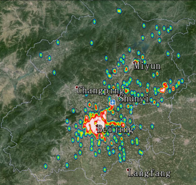
(a) S1: top 563 blocks to place cameras covering all (taxi) vehicles .

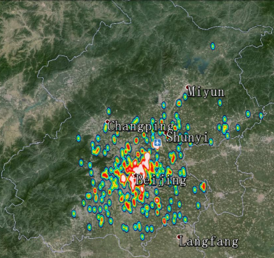
(b) S2: top 563 blocks to place cameras maximizing VCR.

Figure 1: Example camera placement heatmaps derived using one-week taxi data in Beijing based on strategy S1 and S2.

IV-B2 Result Analysis

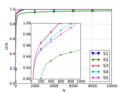
(a) UCR

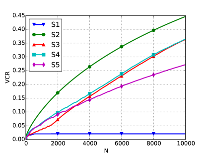
(b) VCR

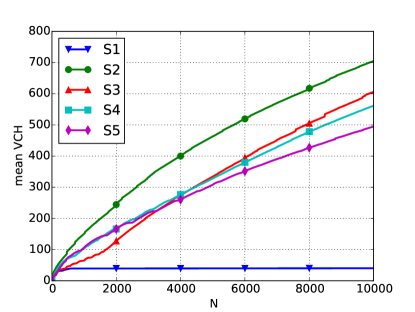
(c) mean VCH

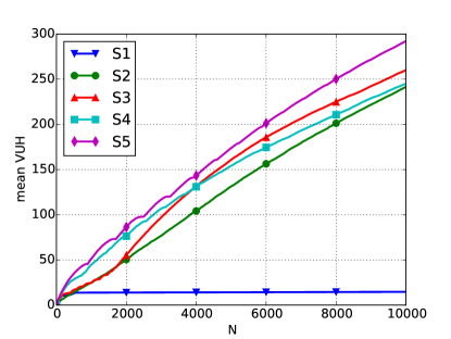
(d) mean VUH

Figure 2: The performance metrics over the number of cameras $N$ of different placement strategies.

For each strategy, we calculate UCR, VCR and VIT by varying the number of cameras $N$ from 1 to 10,000. UCR and VCR reveal the proportion of unique vehicles and vehicle traffic that could be covered under each strategy, respectively. Additionally, we calculate VIT, VCH and VUH for each vehicle to have a closer look at the total amount time when a vehicle is under surveillance, the total number of cameras that a vehicle hits, and the total number of unique cameras that a vehicle hits, respectively.

Fig. 2 depicts the performance of all strategies. Generally, the metrics increase slower as $N$ becomes larger, meaning that all strategies accomplish diminishing returns. Particularly, all metrics rise rapidly before $N$ reaches 200, accounting for no more than 0.05% of all possible blocks where we can place cameras (i.e., $R$).

As Fig. 2a shows, a very small proportion of cameras need to be placed to cover the vast majority of vehicles. Specifically, all strategies exhibit a rapid rise in UCR to at least 90% before $N$ reaches 200, indicating that we need to place cameras in no more than 0.05% blocks to cover at least 90% vehicles. Moreover, all strategies except S2 achieve a 100% UCR before $N$ reaches 900 (i.e., 0.2% of $R$), while S2 almost has no increasing returns after $N=4,000$.

Insight 1. To cover all vehicles, we need to place cameras only in 0.2% blocks at most using S1, S3, S4, S5. Among these strategies capable of covering all vehicles, S1 could cover all vehicles with the smallest $N$ (i.e., the most quickly), followed by S3, S4, and S5 in ascending order. However, S2 could hardly converge to cover all vehicles as $N$ increases.

This insight reveals the existence of a small set of “core” blocks covering all vehicles. Fig. 1a shows the minimum set of such “core” blocks derived from strategy S1. Meanwhile, $S2$ that only maximizes vehicle traffic coverage results in slow or even incomplete vehicle coverage.

Fig. 2b demonstrates the vehicle traffic coverage ratio, where VCR rises roughly linearly as $N$ increases for all strategies exclusive of S1. Among all strategies, S2 exhibits the largest growth rate, followed by S4, S3, S5, and S1. Fig. 1b shows top 563 blocks where we can place cameras to maximize VCR using S2. We observe that the blocks in Fig. 1b are significantly less geographically dispersed than those in Fig. 1a. The growth rates of S3 and S4 are comparable. S1 almost has no increasing returns after $N=200$, implying that an emphasis on vehicle coverage may fail to maximize traffic coverage.

Insight 2. Although S1 achieves the best performance regarding UCR, its performance regarding VCR degrades drastically to an extent where no increasing returns is accomplished when we invest more cameras after $N=200$. In contrast, S3$\sim$S5 achieve significant increasing returns regarding VCR as $N$ increases. Although their increasing returns are not as fast as that of S2, they can converge to cover all vehicles quickly while S2 cannot.

This insight reveals that our proposed strategies S3$\sim$S5 can achieve well-balanced performance between UCR and VCR. This is because they encourage more vehicles under surveillance while simultaneously considering more (unique) camera hits and traffic coverage per vehicle.

Fig. 2c presents mean VCH across all vehicles, which has similar trend as VCR. This reflects that the number of camera hits is positively correlated to in-camera time. For the same reason, VIT exhibits the same trend as VCH. We therefore omit the plot of mean VIT. Among all the strategies, S2 achieves the best average surveillance performance (i.e., longer in-camera time, more camera-hits) per vehicle, though it may result in slow or even incomplete vehicle coverage. Despite the performance degradation in mean VCH compared to S2, strategies S3$\sim$S5 achieve median values of VIT and VCH across all vehicles comparable to S2, while simultaneously exhibiting much smaller standard deviation of VIT and VCH. Furthermore, the Gini coefficient of VCH for $S2$ is larger than that for S3$\sim$S5, confirming that S3$\sim$S5 achieve relatively fairer surveillance across all vehicles regarding in-camera time and camera hits than S2.

Insight 3. S3$\sim$S5 achieve more balanced surveillance across all vehicles in terms of in-camera time and camera hits than S2, avoiding little surveillance of some vehicles and too much surveillance (possibly unnecessary) of others. Therefore, they provide relatively fairer security surveillance services across all vehicles.

Fig. 2d presents the performance of mean VUH (i.e., the number of unique vehicles that a vehicle hits) across all vehicles. We observe that S5 achieves the largest mean VUH, while S1 has no increasing returns after $N$ reaches 200. The remaining strategies exhibit moderate performance worse than that of S5. Actually, S5 encourages deploying cameras in the blocks where different blocks along a vehicle’s trajectory can be observed as many as possible, and meanwhile vehicles can be observed as many as possible. In this case, a vehicle is expected to be observed in more different blocks, thereby beneficial to capturing more places where a vehicle has ever been. This is important in security surveillance that prefers the knowledge on the places where a vehicle has been.

Insight 4. S5 is a strategy in favor of capturing more places where a vehicle has ever been. Other strategies perform worse than S5 regarding mean VUH.

IV-C A Case Study of Randomized Resolution Upgrading

To demonstrate the performance of randomized resolution upgrading based on game theory, we consider a security surveillance scenario where $N=10,000$ cameras are placed while only 1,000 cameras could be of high resolution. Suppose the surveillance focuses on criminal (or terrorist) activities that tend to be conducted at places that are generally with more vehicle traffic (so to make more serious consequences). We thus measure the importance of a block $c_{i}$ according to its amount of traffic in the dataset, which is calculated as $T(c_{i})=\sum_{v\in V}T_{v}(\{c_{i}\})$.

We consider that the defender and the adversary play a zero-sum game. That is, each player’s gain (or loss) of utility is exactly balanced by the losses (or gains) of the utility of the other player(s). Formally, we set $R_{i}^{d}+P_{i}^{a}=0$, $R_{i}^{a}+P_{i}^{d}=0$. Obviously, we have $U^{d}+U^{a}=0$. Meanwhile, the importance values of blocks are normalized through dividing each value by the maximum value. Therefore, we have $R_{i}^{d},R_{i}^{a}\in[0,1]$, and $P_{i}^{d},P_{i}^{a}\in[-1,0]$. Combining (8), (9), (11), and (12), it is easy to know $U^{a},U^{d}\in[-1,1]$.

Before realizing randomized resolution upgrading, we randomly generate 1,000 defender pure strategies in total. The union of these pure strategies cover all the placed cameras to ensure that the resolution of any camera has a chance to be upgraded. On the other hand, an adversary pure strategy is a block where he commits crimes, the number of which equals 10,000.

Table I shows the defender utility (i.e., $U_{d}$) when the defender adopts the mixed strategy, in comparison to adopting two baseline defender strategies, namely, uniform strategy and best strategy. The uniform strategy means the defender adopts a pure strategy uniformly at random. The best strategy allows the defender to constantly adopt the pure strategy that contains the most important block. If there are multiple such pure strategies, the defender selects the one maximizing her utility.

TABLE I: The defender’s expected utility against a best-response adversary under different defender strategies (i.e., mixed strategy, uniform strategy, and best strategy) and different camera placement strategies.

	mixed strategy	baseline strategies
		uniform strategy	best strategy
S1	-0.07313	-0.74600	-0.19582
S2	-0.13279	-0.81400	-0.50654
S3	-0.10210	-0.77800	-0.47290
S4	-0.20533	-0.81000	-0.68853
S5	-0.12091	-0.82800	-0.49978

From the table, we see that the mixed strategy achieves significantly larger utility than the baseline strategies, no matter which placement strategy ($S1\sim S5$) is employed to place the camera infrastructure. Such a result indicates that, once the importance of each block is defined, one can derive the mixed strategy that outperforms baseline strategies and maximizes the defender utility against a sophisticated adversary. This case study implies the feasibility that the security police randomly selects a set of cameras and upgrades their resolution for high-quality video evidence based on the proposed security game model.

V Discussion

V-A Customizing Security Surveillance

Different types of vehicles may require different surveillance priorities. For example, compared with individual cars, taxis (as a public space) and school buses usually need higher surveillance priorities. Although we do not distinguish between different vehicle types, every vehicle $v$ can be assigned a personalized weight $w_{v}$ indicating its surveillance priority, where larger values of the weight indicate higher surveillance priorities. One can also assign weights to vehicles according to their reputation scores derived from social data like accident records and vehicle owners’ criminal records. Vehicles with more accident records, or whose owners have more criminal records, would be assigned higher weights.

The weight $w_{v}$ can be directly used as a multiplier of the parameters in the proposed strategies. For example, $I_{v}(C)$ could be replaced by $w_{v}I_{v}(C)$, and so do $T_{v}(C)$, $H_{v}(C)$ and $U_{v}(C)$. This keeps the non-decreasing submodular property of $F(C)$. Therefore, GA remains applicable. By incorporating individual vehicle information, we can customize placement strategies as needed, with a bias toward vehicles with higher surveillance priorities and lower reputation scores.

V-B Privacy Issues

Determining strategies for customizing security surveillance not only anticipates GPS data sharing from vehicles, but also rely on other social data sources helpful to security surveillance. The data sharing may introduce privacy issues, which however could be resolved by data obfuscation techniques (e.g., obfuscating vehicle IDs). Whenever a security event occurs, the obfuscated data (e.g., vehicles IDs) would again be recovered from collected (video) data recorded by cameras using plate number recognition techniques, after being authorized by privileged authorities. Additionally, tracking individual vehicles by cameras may also have privacy issues. Thus, we suggest the public should be notified of placed cameras, and meanwhile the collected video data MUST be strictly managed by authorities according to law.

VI Related Work

Transportation Monitoring. Transportation monitoring is a broad area closely related to urban computing tasks like energy and transportation optimization (e.g., ridesharing, speed control), road traffic monitoring (e.g., travel time estimation), urban environment modeling (e.g., PM 2.5 air quality) [11]. Transportation monitoring undoubtedly accelerates the operation efficiency of a metropolis. However, none of the existing studies regarding transportation monitoring exploits vehicle traffic to select camera placement blocks in favor of security surveillance.

Physical-World Security Surveillance. Recent years have witnessed a rising trend towards game-theoretic urban security patrolling on roads [12]. Specifically, an adversary assigns different values to reaching (and damaging or destroying) one of multiple targets (e.g., buildings). A defender can allocate resources to capture the attacker before he reaches a target. To prevent attacks, security forces can schedule checkpoints on roads to detect adversaries. Different from these studies, we leverage game theory to control placed cameras. Moreover, camera placement complements road patrolling, because the adversaries missed by the road checkpoints could be further inspected by placed cameras.

VII Conclusion

This article explored the linkage between vehicle traffic and camera placement in favor of security surveillance from a network perspective. We proposed different camera placement strategies that facilitate security surveillance. Using real-world data from a metropolis, we demonstrated that the proposed strategies could facilitate metropolis security surveillance in different aspects. We also studied the security surveillance problem that high-resolution video is desired for high-quality crime evidence, while only a limited number of placed cameras can be of high resolution simultaneously based on game theory. The results illustrated that, using the carefully designed randomized strategy, we can deter a sophisticated adversary with maximal utility under the constraint of practical overhead.

To make our cities safer, there remain a lot of problems to explore. In an era of mass terrorism, we expect our work could stimulate more research on transportation data-driven security surveillance in smart cities.

The submodularity for S3$\sim$S5

Proof.

For the function $F(C)$ defined in S3, given every two sets $C_{1},C_{2}\subseteq\Omega$ and $C_{1}\subseteq C_{2}$, we have

$$F(C_{1})=\Phi-\sum_{v\in V}\left(\frac{S}{T_{v}(C_{1})+1}-1\right)/{|V|}$$

and

$$F(C_{2})=\Phi-\sum_{v\in V}\left(\frac{S}{T_{v}(C_{2})+1}-1\right)/{|V|}.$$

Meanwhile, we add a new block $c\in\Omega\setminus C_{2}$ to $C_{1}$ and $C_{2}$, and obtain

$$F(C_{1}\cup\{c\})=\Phi-\sum_{v\in V}\left(\frac{S}{T_{v}(C_{1}\cup\{c\})+1}-1\right)/{|V|}$$

and

$$F(C_{2}\cup\{c\})=\Phi-\sum_{v\in V}\left(\frac{S}{T_{v}(C_{2}\cup\{c\})+1}-1\right)/{|V|}.$$

Accordingly, we obtain the function value increment as

$$F(C_{1}\cup\{c\}) -F(C_{1})=$$

$$\sum_{v\in V}\left(\frac{S}{T_{v}(C_{1})+1}-\frac{S}{T_{v}(C_{1}\cup\{c\})+1}\right)/{|V|}$$

and

$$F(C_{2}\cup\{c\}) -F(C_{2})=$$

$$\sum_{v\in V}\left(\frac{S}{T_{v}(C_{2})+1}-\frac{S}{T_{v}(C_{2}\cup\{c\})+1}\right)/{|V|}.$$

Recall $T_{v}(C)$ denotes the amount of traffic contributed by $v$ to blocks in $C$. Because of $c\notin C_{1}$ and $c\notin C_{2}$, we have $T_{v}(C_{1}\cup\{c\})=T_{v}(C_{1})+T_{v}(\{c\})$, and $T_{v}(C_{2}\cup\{c\})=T_{v}(C_{2})+T_{v}(\{c\})$. Therefore, the above equations can be rewritten as

$$F(C_{1}\cup\{c\}) -F(C_{1})=$$

$$\sum_{v\in V}\left(\frac{S}{T_{v}(C_{1})+1}-\frac{S}{T_{v}(C_{1})+1+T_{v}(\{c\})}\right)/{|V|}$$

and

$$F(C_{2}\cup\{c\}) -F(C_{2})=$$

$$\sum_{v\in V}\left(\frac{S}{T_{v}(C_{2})+1}-\frac{S}{T_{v}(C_{2})+1+T_{v}(\{c\})}\right)/{|V|}.$$

Given $C_{1}\subseteq C_{2}$, we have $T_{v}(C_{1})\leq T_{v}(C_{2})$ holds. Thus,

$$\left(\frac{S}{T_{v}(C_{1})+1}-\frac{S}{T_{v}(C_{1})+1+T_{v}(\{c\})}\right)$$

$$\geq\left(\frac{S}{T_{v}(C_{2})+1}-\frac{S}{T_{v}(C_{2})+1+T_{v}(\{c\})}\right)$$

Finally, we derive

$$F(C_{1}\cup\{c\})-F(C_{1})\geq F(C_{2}\cup\{c\})-F(C_{2}).$$

The submodularity holds for $F(C)$ defined in S3.

Similarly, we can deduce that the submodularity holds for $F(C)$ defined in S4 and S5. ∎

References

- [1] Alois Stutzer and Michael Zehnder. Is camera surveillance an effective measure of counterterrorism? Defence and Peace Economics, 2013.
- [2] Bandwidth and storage calculator. http://www.stardot.com/bandwidth-and-storage-calculator.
- [3] 2017 Westminster attack. https://en.wikipedia.org/wiki/2017_Westminster_attack.
- [4] G. L. Nemhauser, L. A. Wolsey, and M. L. Fisher. An analysis of approximations for maximizing submodular set functions—I. Mathematical Programming, 1978.
- [5] Andreas Krause and Daniel Golovin. Submodular function maximization. Tractability: Practical Approaches to Hard Problems, 3(19):8, 2012.
- [6] Michał Fularz, Marek Kraft, Adam Schmidt, and Andrzej Kasiński. The architecture of an embedded smart camera for intelligent inspection and surveillance. In Proc. Progress in Automation, Robotics and Measuring Techniques: Control and Automation, 2015.
- [7] Mohammad Hossein Manshaei, Quanyan Zhu, Tansu Alpcan, Tamer Bacşar, and Jean-Pierre Hubaux. Game theory meets network security and privacy. ACM Computing Surveys, 45(3):25:1–25:39, 2013.
- [8] Bo An, Milind Tambe, and Arunesh Sinha. Stackelberg security games (ssg) basics and application overview. In Improving Homeland Security Decisions. Cambridge University Press, 2016.
- [9] Damianos Gavalas, Charalampos Konstantopoulos, Konstantinos Mastakas, and Grammati Pantziou. A survey on algorithmic approaches for solving tourist trip design problems. Journal of Heuristics, 20(3):291–328, 2014.
- [10] T-Drive data. http://research.microsoft.com/apps/pubs/?id=152883.
- [11] Yu Zheng, Licia Capra, Ouri Wolfson, and Hai Yang. Urban computing: Concepts, methodologies, and applications. ACM Transaction on Intelligent Systems and Technology, 2014.
- [12] Yue Yin, Bo An, and Manish Jain. Game-theoretic resource allocation for protecting large public events. In Proc. AAAI AI, 2014.