Iterative Machine Learning for Output Tracking

Abstract

This article develops iterative machine learning (IML) for output tracking. The input-output data generated during iterations to develop the model used in the iterative update. The main contribution of this article to propose the use of kernel-based machine learning to iteratively update both the model and the model-inversion-based input simultaneously. Additionally, augmented inputs with persistency of excitation are proposed to promote learning of the model during the iteration process. The proposed approach is illustrated with a simulation example.

1 Introduction

Iterative learning methods, initially developed in e.g., [1, 2, 3], improve the output-tracking performance by correcting the input based on the measured tracking error. For example, iterative control has led to some of the highest precision for output tracking, e.g., in scanning probe microscopy as demonstrated in, e.g., [4, 5, 6, 7, 8, 9, 10]. Note that sets of learned trajectories can be used to enable tracking of other trajectories, e.g., by designing the feedforward control input using pre-specified basis functions e.g., using polynomial functions [11] or rational functions of the reference trajectory [12]. Similarly, new desired output can be generated by considering different combinations of previously-learned output segments [13] and the feedforward can be represented using radial basis functions that can be optimized for a range of task parameters [14]. This article proposes a kernel-based machine learning approach to use augmented inputs to iteratively learn not just the inverse input $u_{d}$ needed to track a specified output $y_{d}$ but to also use the data acquired during the iteration process to to estimate both (i) the model $\hat{g}$ (and its inverse) for the control update, as well as (ii) the model uncertainty needed to establish bounds on the iteration gain for ensuring tracking-error reduction..

Conditions for convergence of iterative methods have been well studied in literature, e.g., [15, 16, 17, 18, 19, 20, 21, 22, 23, 24]. For example, the need to invert the system $g$ to find the perfect input $u_{d}$ for tracking a desired output $y_{d}$ has motivated the use of the inverse $\hat{g}^{-1}$ of the known model $\hat{g}$ of the system $g$ in early iterative control development [3]. Since convergence depends on the size of modeling error, improvements of the model through parameter adaptation with data acquired during the iteration was studied in, e.g., [25] for robotics application using a discrete-time implementation. Here, for each iteration step, the sampled input vector is mapped to the sampled output vector through a lower triangular matrix map. A stochastic version using such a lower-triangular map has been studied in [26]. Even in the ideal case with no modeling uncertainty, the inverse of this matrix map leads to a stable inverse only if the system is minimum-phase (i.e., no zeros on the right hand side of the complex plane), e.g., [19, 27]. This restriction to minimum-phase systems also applies to the use of input-output data to estimate models that enhance portability of the data-based learning to other output trajectories, e.g., [25, 27]. The extension of iterative learning control for nonminimum phase systems using the noncausal inverse was initially proposed in [20]. The frequency domain implementation of the noncausal inverse was studied in, e.g., [16, 17], and discrete-time implementation was developed in [28], where noncausality was allowed by using full matrices for the input-output map and rational basis functions were used to enable portability between different trajectories in [29]. Convergence to the desired output can be guaranteed (with the frequency domain approach) if the phase uncertainty in the model is less than $90$ degrees and the iteration gain is sufficiently small [16, 18]. Such dependence on the phase uncertainty was also developed using a discrete Fourier transform approach in [17, 30].

Convergence cannot be guaranteed in regions of the frequency domain where the phase uncertainty in the model $\hat{g}$ is greater than $90$ degrees. Frequency regions where convergence cannot be guaranteed can be reduced by using the input-output data generated during the iteration procedure [31]. In particular, more recent model-less approaches use the input-output data from previous iteration steps to avoid the need to model the system explicitly and improve the convergence of the iterative approach [31, 32]. Nevertheless, such input-output data might have substantial error at some frequencies where the signal to noise ratio is small. Kernel-based Gaussian process regression (GPR) [33] is well suited to such function-estimation from noisy data. This motivates the main contribution of the article —  the use of a kernel-based iterative machine learning (IML) approach to predict the magnitude and phase response of the system as functions of frequency from the measured input-output data. An added advantage is that the IML approach also yields the anticipated model uncertainty, which can be used to design the iteration law using previous results from [16, 17, 18].

A second contribution of this article is to propose the use of additional input to the iteration law for persistency of excitation to enhance the model learning. It is shown in the article that convergence cannot be guaranteed if the size of the model is small compared to the size of the error in the model data, e.g., due to noise in the output. The effect of the noise in output measurement can be reduced by increasing the size of the output by using larger input. This increase in the output-to-noise ratio, i.e., the ratio of measured output to known input in the frequency domain, reduces the error in the model data and improves the performance of the iteration procedure. Therefore, this article proposes the injection of additional input into the iteration law whenever the the input size falls below a threshold value. This persistence of excitation leads to smaller noise in the measured system-model data with the proposed approach. (The effect of this input augmentation is removed from the measured output, using the estimated model, before the input is updated at the next iteration step.) Note that similar use of input augmentation to ensure persistency of excitation is commonly used in adaptive control, e.g., [34]. The improved model can be used to better infer the inverse input for new output trajectories. In this sense, the proposed approach enhances the portability of the frequency-domain iterative learning control.

The proposed use of additional input to improve model learning during the iteration process, is general in the sense that it can be used with other modeling methods. For example, in the current work a non-parametric Gaussian process regression (GPR) is proposed to predict the system response from the measured input-output data [33]. However, the proposed model update during the iteration steps can also be applied using parametric methods for modeling, e.g., see recent review in [35]. The models could then be inverted (potentially, in the time domain) during iterations for input update — in contrast, the proposed approach directly measures and stores the frequency data of the model (and hence its inverse). The GPR provides the smoothing in the presence of noisy data. Similarly, there is flexibility in the selection of the kernel used for estimating the models. While the more common smooth squared exponential (SE) kernel is used in this article, the Matern class of kernels could be used for systems with sharper features in the frequency response, e.g., for underdamped systems [33] and the approach could be applied to complex-valued kernels in the frequency domain [36]. The concept of model update in the frequency domain proposed here could be used with spatial-domain iterations, e.g. [37, 38], with model identification methods using repetitive trajectories [39], and with the stable spline kernel for machine learning in the time domain [35] that guarantees bounded-input-bounded-output stability of the resulting models. Finally, the proposed approach can be used to speed up the learning of the different segments in segmented iterative control approaches, e.g., [13].

The paper begins with problem formulation in Section 2, where the standard model-inversion-based iterative control approach is briefly reviewed followed by clarification of the research problem and the proposed solution approach using kernel-based machine learning in Section 3. Convergence conditions are then developed in Section 4, which are used to redesign the iteration law to promote persistency of excitation. Additionally, the overall IML algorithm is presented at the end of Section 4. Simulation results and discussion illustrating the proposed approach are in Section 5 followed by the conclusions in Section 6.

2 Problem formulation

This section begins by discussing the system and limits of the model-inversion approach due to modeling error, followed by background on frequency-domain iterative control to correct for modeling error. Convergence conditions and approaches to reduce the modeling error from data are presented, followed by the research-problem statement.

2.1 Model-based inverse feedforward

Given a desired output $y_{d}$, model inversion can be used to find the feedforward input $u=u_{d}$ that achieves the desired output $y=y_{d}$ for a linear system of the form

$$y(s)=g(s)u(s)$$ (1)

as

$$u_{d}(\omega){} =g^{-1}(\omega)y_{d}(\omega)~{}=[{a}(\omega)+j{b}(\omega)]^{-1}y_{d}(\omega)$$ (2)

with the value of the model $\hat{g}$ evaluated on the imaginary axis of the complex plane defined as $\hat{g}(\omega)=\hat{g}(s){\Huge{|}}_{s=j\omega}$ and $j=\sqrt{-1}$.

Assumption 1 (System properties)

The system $g$ is not identically zero (i.e., it is non-trivial), is stable, and has hyperbolic zero dynamics, i.e., all zeros have a nonzero real parts.

Note that if the known system model $\hat{g}(\omega)$ has error at frequency $\omega$, i.e., $\hat{g}(\omega)\neq g(\omega)$, then the inverse input $\hat{u}_{d}(\omega)$

$$\hat{u}_{d}(\omega)=\hat{g}^{-1}(\omega)y_{d}(\omega)$$ (3)

found using the model $\hat{g}(\omega)$ does not lead to exact output tracking of the desired output $y_{d}(\omega)$, i.e.,

$$g(\omega)\hat{u}_{d}(\omega)~{}=g(\omega)\hat{g}^{-1}(\omega)y_{d}(\omega)~{}\neq y_{d}(\omega).$$ (4)

2.2 Fixed-model-based iterative control

The tracking error caused by the modeling error, $\hat{g}(\omega)\neq g(\omega)$ at frequency $\omega$, can be corrected iteratively, e.g., as [18, 17]

$$u_{k}(\omega)~{}=u_{k-1}(\omega)+\rho_{k}(\omega)\hat{g}_{k}^{-1}(\omega)\left[y_{d}(\omega)-y_{k-1}(\omega)\right]$$ (5)

provided $\hat{g}_{k}^{-1}(\omega)\neq 0$ at frequency $\omega$, where at each integer iteration-step $k>1$, the input $u_{k}$ is computed using Eq. (5) with a real-valued scalar, frequency-dependent, iteration gain $\rho_{k}$ and the available system model $\hat{g}_{k}$ and applied to the system to find the output $y_{k}$. Note that the term in the square bracket in Eq. (5) represents the output error. The iterative control in Eq. (5) converges at frequency $\omega$ if the modeling error is sufficiently small, as shown in [18, 17], and stated formally below.

Lemma 1 (Output-tracking convergence)

With a finite initial input $u_{1}(\omega)$, a fixed iteration gain $\rho_{k}(\omega)=\rho(\omega)$, and non-zero system model $\hat{g}_{k}(\omega)=\hat{g}(\omega)\neq 0$ at frequency $\omega$ , the iterations in Eq. (5) converges to the inverse input $u_{d}(\omega)$, i.e.,

$$\lim_{k\rightarrow\infty}u_{k}(\omega)=u_{d}(\omega)~{}=g^{-1}(\omega)\left[y_{d}(\omega)\right],$$ (6)

which results in exact tracking of the desired output $y_{d}(\omega)$, i.e.,

$$\lim_{k\rightarrow\infty}y_{k}(\omega)=\lim_{k\rightarrow\infty}g(\omega)u_{k}(\omega)=y_{d}(\omega),$$ (7)

if and only if the magnitude of the phase uncertainty $\Delta_{p}$ in the model $\hat{g}$ and the iteration gain $\rho$ are sufficiently small

$$|\Delta_{p}(\omega)| <\pi/2$$ (8)

$$0<\rho(\omega) <\frac{2\cos{\left[\Delta_{p}(\omega)\right]}}{\Delta_{m}(\omega)},$$

where the magnitude uncertainty $\Delta_{m}$ and the phase uncertainty $\Delta_{p}$ are defined by

$$\frac{\hat{g}^{-1}(\omega)}{g^{-1}(\omega)}~{}=\frac{g(\omega)}{\hat{g}(\omega)}~{}=\Delta_{m}(\omega)e^{j\Delta_{p}(\omega)}.$$ (9)

Proof: This follows from Lemma 1 in [16, 18]. The phase condition is the same as in  [17]. Briefly, multiplying Eq. (5) by the system $g$ and subtracting from the desired output $y_{d}$ yields

$${y_{d}(\omega)-y_{k}(\omega)}~{}=\left(1-\rho(\omega)\frac{g(\omega)}{\hat{g}(\omega)}\right)\left[{y_{d}(\omega)-y_{k-1}(\omega)}\right],$$ (10)

which will tend to zero with increasing iteration steps $k$ if

$$\left|1-\rho(\omega)\frac{g(\omega)}{\hat{g}(\omega)}\right|=\left|1-\rho(\omega)\Delta_{m}(\omega)e^{j\Delta_{p}(\omega)}\right|<~{}1.$$ (11)

The lemma follows by squaring the right hand side of the above equation to obtain

$$1-2\rho(\omega)\Delta_{m}(\omega)\cos(\Delta_{p}(\omega))+\rho^{2}(\omega)\Delta_{m}^{2}(\omega)<1$$ (12)

and removing one from both sides to yield (since $\Delta_{m}>0$ because $g(\omega)\neq 0$, $\hat{g}(\omega)\neq 0$ ),

$$\rho(\omega)\left[\rho(\omega)\Delta_{m}(\omega)-2\rho(\omega)\cos(\Delta_{p}(\omega))\right]<0.$$ (13)

Note that if the phase uncertainty is small, i.e., $|\Delta_{p}(\omega)|<\pi/2$, then $\cos(\Delta_{p}(\omega))>0$ and $\rho(\omega)$ needs to be positive to satisfy Eq. (13). However, if the phase uncertainty $|\Delta_{p}(\omega)|$ is greater than $\pi/2$, then a fixed $\rho(\omega)$ cannot satisfy Eq. (13) for all uncertainties since $\cos(\Delta_{p}(\omega))$ can potentially be positive or negative. Finally, when $|\Delta_{p}(\omega)|=\pi/2$, the left hand side is positive.  

Remark 1 (Small phase error)

The above condition implies that tracking errors reduce at each iteration step, and the input iterations will converge to the desired inverse input as in Eq. (6) at each frequency $\omega$ if and only if the iteration gain $\rho(\omega)$ is chosen to be sufficiently small, provided the phase error $\Delta_{p}(\omega)$ is less than $90$ degrees [16, 18, 17].

x

2.3 Data-based model update for iterative control

The inverse model $\hat{g}_{k}^{-1}(\omega)$ in the iterative control in Eq. (5), used to compute the input $u_{k}(\omega)$ at iteration step $k$, can be estimated from the previously computed input $u_{k-1}(\omega)$ and the corresponding output $y_{k-1}(\omega)$ as

$$\hat{g}_{k}^{-1}(\omega)~{}=\frac{u_{k-1}(\omega)}{y_{k-1}(\omega)}$$ (14)

if $y_{k-1}(\omega)\neq 0$. Provided the noise in the estimation of the model $\hat{g}_{k}(\omega)$ ($k>1$) is small, the above approach can be used with an iteration gain of $\rho_{k}(\omega)=1$ to modify the iterative input-update law in Eq. (5) to [31]

$$u_{k}(\omega)~{}=\left\{\begin{aligned} &\frac{u_{k-1}(\omega)}{y_{k-1}(\omega)}y_{d}(\omega)&\quad{\mbox{if}}~{}y_{k-1}(\omega)\neq 0\\ &0&\quad{\mbox{otherwise}}\end{aligned}\right.$$ (15)

and the initial input at $k=1$ is considered to be

$$u_{1}(\omega)=\alpha y_{d}(\omega)$$ (16)

where $\alpha$ is a constant that can be chosen, e.g., to be the inverse of the estimated DC gain of the system. The tracking error can be made small if the noise in the measurements is small, as shown in [31].

Remark 2 (Model filtering)

The estimated inverse model $\hat{g}_{k}^{-1}(\omega)$ in the iterative control in Eq. (5) at iteration step $k$ can be replaced by a weighted average from all available estimates from iteration steps $k_{i}\leq k$ to reduce the effect of noise [32].

2.4 The research problem

There are two main issues with current frequency-domain iterative approaches, e.g., [18, 31, 17]. The first issue is that while these frequency-domain methods iteratively find the inverse input $u_{d}$ to achieve a desired output $y_{d}$, they do not directly improve the ability to track a new output trajectory $y_{d,2}$, with potentially different frequency content. Secondly, current approaches do not improve estimates of the uncertainties ($\Delta_{m},\Delta_{p}$) in the model $\hat{g}$. Note that lower model uncertainties can allow the use of larger iteration gains according to Eq. (8) and can lead to faster convergence.

The research problem is to iteratively learn the system model $\hat{g}$ (and therefore, its inverse $\hat{g}^{-1}$) and estimate the model uncertainties ($\Delta_{m},\Delta_{p}$) while iteratively learning the inverse input $u_{d}$ needed to track a desired output $y_{d}$.

3 Proposed machine learning of model

A kernel-based machine learning approach is proposed in this section to learn the system model $\hat{g}$ during the iteration process. The Gaussian process assumption is clarified first in Subsection 3.1, followed by background on the Gaussian process regression (GPR) approach to estimate a general function $f$ in Subsection 3.2, and lastly, by the application of the GPR to estimate the system model in Subsection 3.3.

3.1 Model is assumed to be a Gaussian process

In the following, the real $\hat{a}$ and imaginary $\hat{b}$ components of the model $\hat{g}$ are considered to be independent real-valued Gaussian processes as in [41].

Assumption 2 (Gaussian process)

The real $\hat{a}$ and imaginary $\hat{b}$ components of the system model $\hat{g}$ are considered to be zero-mean, real-valued, independent Gaussian processes with covariance functions $k_{a}(\omega,\omega^{\prime})$ and $k_{b}(\omega,\omega^{\prime})$ respectively, i.e.,

$$\hat{a}(\omega) ={\mathcal{R}}[g(\omega)]\sim GP\left(0,k_{a}(\omega,\omega^{\prime})\right)$$ (17)

$$\hat{b}(\omega) ={\mathcal{I}}[g(\omega)]\sim GP\left(0,k_{b}(\omega,\omega^{\prime})\right),$$

where the measured real $m_{a}$ and imaginary $m_{b}$ components are given by

$$m_{a} =\hat{a}(\omega)+\epsilon_{a}$$ (18)

$$m_{b} =\hat{b}(\omega)+\epsilon_{b}$$

with additive, zero-mean, independent identically distributed Gaussian noise $\epsilon_{a},\epsilon_{b}$ with variance $\sigma_{a}^{2},\sigma_{b}^{2}$.

Remark 3 (Lack of knowledge about the model)

The Gaussian process has zero mean in Assumption 2 — the estimated model $\hat{g}(\omega)$ tends to zero at frequencies $\omega$ far from the frequency region where data is available. The size of the acceptable modeling uncertainty (for using inversion-based input update) depends on the estimated model size, as discussed in the next section.

Remark 4 (Related real and imaginary components)

The real and imaginary components of a causal linear transfer function ${g}$ are related to each other by the Kramers-Kronig relations, e.g., [42]. However, this relation between the real and imaginary components is not pointwise in frequency. For example, the real part $\hat{a}(\omega)$ at a frequency $\omega$ depends on the complex part $\hat{b}(\cdot)$ over the entire frequency domain. The approach used here to separately estimate the real $\hat{a}$ and imaginary $\hat{b}$ components of the model $\hat{g}$ is conservative and over-predicts the uncertainty. Therefore, it can lead to a smaller iteration gain $\rho$ with slower convergence.

3.2 Background: Gaussian process regression

The data-based estimation of the expected value general function $f(\cdot)$ with $n$ measurements $m\in{\cal{R}}_{n}$ at frequencies $\Omega\in{\cal{R}}_{n}$ at frequency $\omega\in{\cal{R}}$ using Gaussian process regression (GPR) is stated formally in the following lemma, e.g., [33].

Lemma 2 (Machine learning)

Let $f$ be a zero-mean real-valued Gaussian process over the frequency space

$$f(\omega)\sim GP\left(0,k(\omega,\omega^{\prime})\right)$$ (19)

with covariance function $k(\omega,\omega^{\prime})$, and measurements $m\in{\cal{R}}_{n}$ given by

$$m~{}=f(\omega)+\epsilon$$ (20)

with additive, zero-mean, independent identically distributed Gaussian noise with variance $\sigma^{2}$. Then, the prediction ${f_{\star}}$ at any prediction frequency $\omega\in{\cal{R}}$, given $n$ measured data

$${\bf{m}}=\left[m_{1}~{}m_{2}~{}\ldots~{}m_{n}\right]^{T}$$ (21)

(with the superscript $T$ indicating matrix transpose) at frequencies

$$\Omega=\left[\omega_{1}~{}\omega_{2}~{}\ldots~{}\omega_{n}\right]^{T},$$ (22)

is Gaussian [33]

$${f_{\star}}{\Huge{|}}\Omega,{\bf{m}},\omega~{}\sim{\mathcal{N}}\left(\bar{f_{\star}},\sigma_{f_{\star}}^{2}\right),$$ (23)

where the predicted mean $\bar{f_{\star}}$ and variance $\sigma_{f_{\star}}^{2}$ at any prediction frequency $\omega$ are given by

$$\bar{f_{\star}}(\omega){} ~{}=K(\omega,\Omega)\left[K(\Omega,\Omega)+\sigma^{2}I\right]^{-1}{\bf{m}}$$ (24)

$$\sigma_{f_{\star}}^{2}(\omega){} ~{}=K(\omega,\omega)$$

$$\quad-K(\omega,\Omega)\left[K(\Omega,\Omega)+\sigma^{2}I\right]^{-1}K(\Omega,\omega)$$

with $K(\Omega,\omega)$ denoting the covariances evaluated at all pairs of measured frequencies $\Omega\in{\cal{R}}_{n}$ and the prediction frequency $\omega\in{\cal{R}}$. The other covariance matrices $K(\cdot,\cdot)$ are defined similarly.

Proof: See, e.g., Chapter 2 in [33].  

3.3 Estimation of model from data

The data-based estimation of the real $\hat{a}$ and imaginary $\hat{b}$ components of the system model $\hat{g}$ using GPR from the above Lemma 2, e.g., [33] is described below.

At iteration step $k$, given all the measured real ${\bf{m}}_{a,k}$ and imaginary ${\bf{m}}_{b,k}$ components at frequencies $\Omega_{k}$, the predictive means $\bar{a}_{\star,k}(\omega),\bar{b}_{\star,k}(\omega)$ and variances $\sigma_{a_{\star,k}}^{2}(\omega),\sigma_{b_{\star,k}}^{2}(\omega)$ of the real $a(\omega)$ and imaginary $b(\omega)$ components at prediction frequency $\omega$ can be obtained by setting

$${f_{\star}}={z}_{\star,k},\quad\sigma_{f_{\star}}=\sigma_{{z}_{\star,k}},\quad{\bf{m}}={\bf{m}}_{z,k},\quad\Omega=\Omega_{k}$$ (25)

in Eq. (23) and Eq. (24) of the above Lemma 2 where the subscript $z$ is replaced by either $a$ or $b$ depending on whether the real or imaginary component is being predicted.

The resulting model $\hat{g}_{k}$ at the $k^{th}$ iteration step is given by

$$\hat{g}_{k}(\omega) ~{}=[\bar{a}_{\star,k}(\omega)+j\bar{b}_{\star,k}(\omega)]~{}:=[\hat{a}_{k}(\omega)+j\hat{b}_{k}(\omega)].$$ (26)

4 Convergence with machine learned model

Convergence of the iterative approach with the estimated model from machine learning can be quantified in terms of the size of the model uncertainties in its real $\hat{a}_{k}$ and imaginary $\hat{b}_{k}$ components, as shown in this section. This is followed by a discussion on the augmentation of the iterative input law (at frequencies where the signal to noise ration is low) to reduce the impact of measurement noise when estimating the model. This section concludes with the proposed algorithm.

4.1 Convergence under bounded uncertainties

4.1.1 Convergence conditions

In the following lemmas, it is assumed that the size of the model uncertainty is bounded.

Condition 1 (Bounds on model uncertainty)

The deviations of the real and imaginary components $a,b$ of the system in Eq. (2) from the corresponding components $\hat{a}_{k},\hat{b}_{k}$ of the model in Eq. (26) at iteration step $k$, are bounded as

$$|a(\omega)-\hat{a}_{k}(\omega)| ~{}~{}\leq\Delta_{a,k}(\omega)$$ (27)

$$|b(\omega)-\hat{b}_{k}(\omega)| ~{}~{}\leq\Delta_{b,k}(\omega).$$

Remark 5 (Confidence intervals)

Predictive confidence intervals can be used as bounds on the model uncertainties in Eq. (27). In this probabilistic setting, the chance of not converging can be made small, but the method does not guarantee that the tracking error will decrease. Nevertheless, if the model uncertainty falls outside of the specified confidence intervals at frequency $\omega$ and the input $u_{k}(\omega)$ starts to grow, then the resulting output $y(\omega)$ will also become large due to the hyperbolic-internal dynamics $g(\omega)\neq 0$ from Assumption 1. If the output error becomes large compared to the noise in the measurement at some frequency $\omega$, then this yields additional data at frequency $\omega$ for improved model estimation, and input correction.

Conditions on the magnitude and phase uncertainties can be developed based on the uncertainties in the real and imaginary components of the model, as shown below.

Lemma 3 (Bounds on phase and magnitude)

Under Condition 1, the magnitude uncertainty $\Delta_{m,k}(\omega)$ and the phase uncertainty $\Delta_{p,k}(\omega)$, similar to Eq. (9),

$$\Delta_{m,k}(\omega)e^{j\Delta_{p,k}(\omega)}~{}=~{}\frac{g(\omega)}{\hat{g}_{k}(\omega)}=~{}\frac{a(\omega)+jb(\omega)}{\hat{a}_{k}(\omega)+j\hat{b}_{k}(\omega)}$$ (28)

satisfy

$$|\Delta_{m,k}(\omega)|~{}\leq\frac{|\Delta_{k}(\omega)+\hat{g}_{abs,k}(\omega)|}{|\hat{g}_{k}(\omega)|}$$ (29)

and

$$\cos[{\Delta_{p,k}}(\omega)]~{}\geq\frac{|\hat{g}_{k}(\omega)|^{2}-\hat{g}_{abs,k}(\omega).\Delta_{k}(\omega)}{|\hat{g}_{k}(\omega)|~{}~{}|\hat{g}_{abs,k}(\omega)+\Delta_{k}(\omega)|},$$ (30)

where

$$\Delta_{k}(\omega) =\Delta_{a,k}(\omega)+j\Delta_{b,k}(\omega)$$ (31)

$$\hat{g}_{abs,k}(\omega) =|\hat{a}_{k}(\omega)|+j|\hat{b}_{k}(\omega)|.$$

Proof: An expression for the magnitude $\Delta_{m,k}$ can be found from the definition in Eq. (28) as

$$\Delta_{m,k}(\omega)~{}=~{}\frac{|g(\omega)|}{|\hat{g}_{k}(\omega)|}$$ (32)

and the condition in Eq. (29) follows since the numerator is maximized by selecting the maximial $|a(\omega)|,|b(\omega)|$ that satisfy the lemma’s condition in Eq. (27), as in Eq. (29). The cosine of the phase angle between the model $\hat{g}_{k}(\omega)$ and the system $g(\omega)$ can be found using the dot product as

$$\cos[{\Delta_{p,k}}(\omega)]~{}=\frac{\hat{g}_{k}(\omega).g(\omega)}{|\hat{g}_{k}(\omega)|~{}|g(\omega)|}.$$ (33)

The numerator in Eq. (33)

$$\hat{g}_{k}(\omega).g(\omega) =\hat{a}_{k}(\omega)a(\omega)+\hat{b}_{k}(\omega)b(\omega)$$ (34)

$$=\hat{a}_{k}^{2}(\omega)+\hat{b}_{k}^{2}(\omega)+\delta_{a,k}(\omega)\hat{a}_{k}(\omega)+\delta_{b,k}(\omega)\hat{b}_{k}(\omega),$$

where

$$a(\omega)=\hat{a}_{k}(\omega)+\delta_{a,k}(\omega), b(\omega)=\hat{b}_{k}(\omega)+\delta_{b,k}(\omega)$$ (35)

$$|\delta_{a,k}(\omega)|\leq\Delta_{a,k}(\omega), |\delta_{b,k}(\omega)|\leq\Delta_{b,k}(\omega)$$

is minimized (can be negative) when $\delta_{a,k}$ and $\delta_{b,k}$ are chosen as

$$\delta_{a,k}(\omega) =-[\operatorname{sgn}{\hat{a}_{k}(\omega)}]\Delta_{a,k}(\omega)$$ (36)

$$\quad\delta_{b,k}(\omega) =-[\operatorname{sgn}{\hat{b}_{k}(\omega)}]\Delta_{b,k}(\omega),$$

which results in

$$\hat{g}_{k}(\omega).g(\omega)=\hat{a}_{k}^{2}(\omega)+\hat{b}_{k}^{2}(\omega)-\Delta_{a,k}(\omega)|\hat{a}_{k}(\omega)|-\Delta_{b,k}(\omega)|\hat{b}_{k}(\omega)|$$ (37)

and the numerator in the right hand side of Eq. (30). The denominator in Eq. (33) is maximized when the system magnitude $|g(\omega)|$ is the largest possible, i.e., from Eq. (35)

$$\delta_{a,k}(\omega) =[\operatorname{sgn}{\hat{a}_{k}(\omega)}]\Delta_{a,k}(\omega)$$ (38)

$$\quad\delta_{b,k}(\omega) =[\operatorname{sgn}{\hat{b}_{k}(\omega)}]\Delta_{b,k}(\omega),$$

which results in the denominator in the right hand side of Eq. (30). Minimizing the numerator and maximizing the denominator of Eq. (33) results in the lemma’s claim in Eq. (30).

 

Next, an iterative control law is designed to reduce the tracking error when the model uncertainties satisfy the bounds in Condition 1.

Lemma 4 (Error reduction with iteration)

Under Condition 1, and non-zero system model $\hat{g}_{k}(\omega)\neq 0$ at frequency $\omega$, the iteration law in Eq. (5) reduces the tracking error, i.e.,

$$|y_{d}(\omega)-y_{k}(\omega)|<|y_{d}(\omega)-y_{k-1}(\omega)|$$ (39)

provided the iteration gain $\rho_{k}$ satisfies

$$0<\rho_{k}<2\frac{|\hat{g}_{k}(\omega)|^{2}-\hat{g}_{abs,k}(\omega).\Delta_{k}(\omega)}{|\hat{g}_{abs,k}(\omega)+\Delta_{k}(\omega)|^{2}}=\rho_{k}^{*}(\omega).$$ (40)

Proof: From Eqs. (29),  (30) and  (40)

$$0<\rho_{k}(\omega)<\rho_{k}^{*}(\omega)\leq 2\frac{\cos[{\Delta_{p,k}}(\omega)]}{\Delta_{m,k}(\omega)}.$$ (41)

Since ${\Delta_{m,k}(\omega)}>0$ (from Eq. (32), as the model $\hat{g}_{k}(\omega)$ and the system ${g}_{k}(\omega)$ are assumed to be non-zero at frequency $\omega$),

$$\rho_{k}(\omega){\Delta_{m,k}(\omega)}-2{\cos[{\Delta_{p,k}}(\omega)]}<0$$ (42)

and as $\rho_{k}(\omega)>0$ from Eq. (41),

$$\rho_{k}(\omega){\Delta_{m,k}(\omega)}\left[\rho_{k}(\omega){\Delta_{m,k}(\omega)}-2{\cos[{\Delta_{p,k}}(\omega)]}\right] <0$$ (43)

$$1+\rho_{k}(\omega){\Delta_{m,k}(\omega)}\left[\rho_{k}(\omega){\Delta_{m,k}(\omega)}-2{\cos[{\Delta_{p,k}}(\omega)]}\right] <1.$$

Then, using re-arrangement of the terms similar to those in Eqs. (11) and (12), results in

$$\left|1-\rho_{k}(\omega)\frac{g(\omega)}{\hat{g}_{k}(\omega)}\right|<~{}1$$ (44)

and the lemma follows from Eq. (10) with the iteration gain $\rho_{k}(\omega)$.  

Remark 6 (Iteration gain)

A large iteration gain can result in a large tracking-error reduction but it can also amplify the effect of noise [18]. Iteration gains larger than one can lead to oscillatory convergence. In the following, the iteration gain $\rho_{k}(\omega)$ is selected to satisfy the upper bound $\rho_{k}^{*}(\omega)$ in Eq. (41), as

$$\rho_{k}(\omega)=\underline{\rho}(\omega)\min\left\{\rho_{k}^{*}(\omega),1\right\}~{}<\rho_{k}^{*}(\omega),$$ (45)

with $\underline{\rho}(\omega)\in(0,1)$.

Remark 7 (Convergence with varying iteration gain)

While the tracking error is decreasing as in Eq. (39), the rate of decrease can also potentially decrease with a varying iteration gain $\rho_{k}(\omega)$, e.g., $\rho_{k}(\omega)\rightarrow 0$. Nevertheless, if the modeling uncertainties decrease with additional data, $g_{k}(\omega)\rightarrow g(\omega)$, then the upper bound on the iteration gain increases $\rho_{k}^{*}\rightarrow 2$ from Eq. (41) and the iteration gain in Eq. (45) stays bounded away from zero, with $\rho_{k}(\omega)\rightarrow\underline{\rho}(\omega)$. Alternatively, the model updates and changes in the iteration gains could be stopped after a fixed number of iterations, say $k=k_{pe}$, for guaranteed output-tracking convergence as in Lemma 1

4.1.2 Zero iteration gain for large model uncertainty

Guaranteed convergence of the iteratively found input $u_{k}(\omega)$ to the desired inverse input $u_{d}(\omega)$ at frequency $\omega$, i.e., $u_{k}(\omega)\rightarrow u_{d}(\omega)$ in Eq. (6), depends on the model uncertainties $\Delta_{a,k}(\omega),\Delta_{b,k}(\omega)$ being smaller than the size of the model $|\hat{a}_{k}(\omega)|,|\hat{b}_{k}(\omega)|$. Therefore, the upper bound on the iteration gain $\rho_{k}^{*}(\omega)$ becomes zero if the uncertainties are large, as stated in the lemma below.

Lemma 5 (Large uncertainty)

If the uncertainties $\Delta_{m,k}(\omega),\Delta_{p,k}(\omega)$ in the real $\hat{a}_{k}(\omega)$ and imaginary $\hat{b}_{k}(\omega)$ components of the model $\hat{g}_{k}$ are larger than the size of the model components, i.e.,

$$\Delta_{a,k}(\omega) ~{}~{}\geq|\hat{a}_{k}(\omega)|$$ (46)

$$\Delta_{b,k}(\omega) ~{}~{}\geq|\hat{b}_{k}(\omega)|,$$

then, the upper bound $\rho_{k}^{*}(\omega)$ on the iteration gain in the convergence condition in Eq. (40) of Lemma 4 is zero

$$\rho_{k}^{*}(\omega)=0.$$ (47)

Proof: The lemma follows since, the uncertainty $\Delta_{k}(\omega)=\hat{g}_{abs,k}(\omega)$, as defined in Eq. (33), satisfies Eq. (46) and results in

$${|\hat{g}_{k}(\omega)|^{2}-\hat{g}_{abs,k}(\omega).\Delta_{k}(\omega)}=0.$$ (48)

 

Remark 8 (Magnitude and phase uncertainties)

If the uncertainties $\Delta_{m,k},\Delta_{p,k}$ in the real $\hat{a}_{k}$ and imaginary $\hat{b}_{k}$ components of the model $\hat{g}_{k}$ are larger than the size of the model components, i.e., as in Eq. (46), the magnitude uncertainty $\Delta_{m,k}(\omega)$ can become infinite in Eq. (29) and the cosine of the phase uncertainty $\cos[{\Delta_{p,k}}(\omega)]$ cannot be guaranteed to be greater than zero in Eq. (30), i.e., the phase uncertainty ${\Delta_{p,k}}(\omega)$ cannot be guaranteed to be less than $90^{o}$. These are required for guaranteed reduction in the output tracking error with iterations in previous results in [18, 17], e.g., as in Remark 1.

Remark 9 (Similar conditions to robust inversion)

The requirement, that the uncertainties $\Delta_{m,k}(\omega),\Delta_{p,k}(\omega)$ in the model components $\hat{a}_{k}(\omega),\hat{b}_{k}(\omega)$ should be smaller than the size of the model components to ensure a nonzero iteration gain as in Lemma 5, is similar to condition that the model uncertainty be smaller than the size of the model for robust invertibility [40].

Remark 10 (Limited tracking beyond system bandwidth)

At frequencies $\omega$ much higher than the system bandwidth $\omega_{bw}$, typical system model magnitudes $|\hat{g}(\omega)|$ tend to become small. Therefore, for a given level of model uncertainties $\Delta_{a,k}(\omega),\Delta_{b,k}(\omega)$ (due to noise in the measurements), the upper bound $\rho^{*}(\omega)$ on the iteration gain in Eq. (40) tends to be zero at high frequencies $\omega>>\omega_{bw}$.

4.2 Iteration law with persistency of excitation

Sufficient richness of the measured system-model and reduced error in the model data can be achieved by augmenting the input ${u}_{k}(\omega)$ with an additional term $\tilde{u}_{k}(\omega)$ that ensures persistency of excitation at a frequency $\omega$ even if the desired output $y_{d}(\omega)$, and therefore the feedforward input $u_{d}(\omega)$ in Eq. (2) are zero at that frequency $\omega$ .

4.2.1 Modified iteration

The iterative law in Eq. (5) is modified to

$$\hat{u}_{k}(\omega){} =[u_{k-1}(\omega)-\tilde{u}_{k-1}(\omega)]$$ (49)

$$+\rho_{k}(\omega)\hat{g}_{k}^{-1}(\omega)\left[y_{d}(\omega)-({y}_{m,k-1}(\omega)-\tilde{y}_{m,k-1}(\omega))\right]$$

$$u_{k}(\omega){} =\hat{u}_{k}(\omega)+\tilde{u}_{k}(\omega)$$

for $\omega\leq\omega_{c}$ and zero elsewhere. Here the additional input $\tilde{u}_{k}(\omega)$ is used whenever the un-augmented input $\hat{u}_{k}(\omega)$ becomes small to provide persistence of excitation, in the first $k_{pe}<k^{*}$ iterations, where $k^{*}$ is the total number of iteration steps. For example, the additional input can be chosen to have magnitude $\tilde{u}(\omega)$ and a random phase angle $\phi_{k}$, i.e.,

$$\tilde{u}_{k}(\omega){} =\left\{\begin{aligned} &\tilde{u}(\omega)e^{j[\phi_{k}(\omega)]}&\quad&{\mbox{if}}~{}|\hat{u}_{k}(\omega)|<u_{pe}(\omega)\\ &&&{\mbox{and }}~{}k\leq k_{pe}\\ &0&\quad&{\mbox{otherwise}}\end{aligned}\right.$$ (50)

$$\phi_{k}(\omega){} \sim{\mathcal{N}}\left(0,\pi^{2}\right),$$

where $u_{pe}(\omega)$ is selected to designate when the input is considered to be small. Note that the additional input $\tilde{u}_{k-1}(\omega)$ from the previous iteration is removed when updating the iterative input $u_{k}(\omega)$ in Eq. (49). Moreover, the estimated effect $\tilde{y}_{m,k-1}(\omega)$ of the additional input $\tilde{u}_{k-1}(\omega)$ on the measured output $y_{m,k-1}(\omega)$ is removed before computing the updated input $u_{k-1}(\omega)$ in Eq. (49), with

$$\tilde{y}_{m,k-1}(\omega){} =\hat{g}_{k}(\omega)\tilde{u}_{k-1}(\omega),$$ (51)

where the measured output $y_{m,k-1}(\omega)$ includes potential measurement noise $n_{y,k-1}(\omega)$, i.e.,

$$y_{m,k-1}(\omega){} =y_{k-1}(\omega)+n_{y,k-1}(\omega)$$ (52)

$$n_{y,k-1}(\omega){} \sim{\mathcal{N}}\left(0,\sigma_{y,a}^{2}(\omega)\right)+j{\mathcal{N}}\left(0,\sigma_{y,b}^{2}(\omega)\right).$$

Remark 11 (Residual modeling error)

If the model is not learned well, then the correction of the input augmentation in Eq. (51) will not be exact. The error due to in-exact compensation of the input augmentation can be corrected iteratively if the total number of iterations $k^{*}$ is sufficiently larger than the initial iterations $k\leq k_{pe}$ when the input is augmented, i.e., $k_{pe}<<k^{*}$.

If an initial model $\hat{g}_{1}$ is available, then the output-tracking input can be estimated as

$$\hat{u}_{1}(\omega){} =\hat{g}_{1}^{-1}(\omega)\left[y_{d}(\omega)\right]~{}~{}\forall~{}\omega\leq\omega_{c},$$ (53)

and zero elsewhere. If an initial model is not available, then $\hat{u}_{1}(\omega)=0$ for all frequency $\omega$. The input $\hat{u}_{1}$ can be augmented to improve model estimation, as

$$u_{1}(\omega){} =\hat{u}_{1}(\omega)~{}+\tilde{u}_{1}(\omega),\quad~{}~{}\forall~{}\omega\leq\omega_{c},$$ (54)

and zero elsewhere, with $\tilde{u}_{1}$ as in Eq. (50).

Remark 12 (Initial input using learned model)

The final model $\hat{g}_{k^{*}}$ at the final iteration step ${k^{*}}$ can be used as the initial model $\hat{g}_{1}$ in Eq. (54) during the iterative output tracking of a new output trajectory $y_{d,2}$.

4.2.2 Additional data for model

New data $m_{a,k}(\omega),m_{b,k}(\omega)$ to estimate the system model $\hat{g}_{k}(\omega)$ can be computed at frequencies $\omega$ where the input $u_{k-1}(\omega)$ is sufficiently large, say

$$|u_{k-1}(\omega)|~{}\geq u_{ok}(\omega)>0,$$ (55)

as in Eq. (18)

$$m_{g,k}(\omega){} ={m}_{a,k}(\omega)+j{m}_{b,k}(\omega)~{}=\frac{y_{m,k-1}(\omega)}{u_{k-1}(\omega)}$$ (56)

$$=\frac{y_{k-1}(\omega)+n_{y,{k-1}}(\omega)}{u_{k-1}(\omega)}$$

$$=g(\omega)~{}+\frac{n_{y,{k-1}}(\omega)}{u_{k-1}(\omega)}$$

with the measurement noise $n_{y,k-1}(\omega)$ as in Eq. (52).

Remark 13 (Reduction of measurement-noise effect)

The magnitude $\tilde{u}(\omega)$ of the additional input at frequency $\omega$ in Eq. (50) should be selected to be much larger than the expected standard deviations $\sigma_{y,a}(\omega),\sigma_{y,b}(\omega)$ of the measurement noise $n_{y,k-1}(\omega)$ in Eq. (52) to increase the input $u_{k-1}(\omega)$ and reduce the impact of measurement noise $n_{y,k-1}(\omega)$ on the model data ${m}_{a,k}(\omega),{m}_{b,k}(\omega)$ computed using Eq. (56).

4.2.3 Averaged model data

The computational cost of GPR can become prohibitive as the number of model data increases, e.g., with increasing iteration steps. Therefore, in the proposed algorithm, the model data is first averaged at each frequency $\omega$ where $N_{\omega,k}>0$ data points are available similar to [32], as discussed in Remark 3,

$$\bar{m}_{g,k}(\omega)~{}=\bar{m}_{a,k}(\omega)+j\bar{m}_{b,k}(\omega)=\frac{1}{N_{\omega,k}}\sum_{i=1}^{k}m_{g,i}(\omega)$$ (57)

and $m_{g,i}$ is defined in Eq. (56). Then, the averaged data $\bar{m}_{g,k}(\omega)$ is used to refine the model $\hat{g}_{k}$ using the GPR in Eq. (24) before computing the updated input $u_{k}(\omega)$ in Eq. (49). With sufficient number of data points $N_{\omega,k}$ at a frequency $\omega\leq\omega_{c}$ due to persistency of excitation, the estimated mean $\bar{m}_{g,k}(\omega)$ of the model data tends to the system $g(\omega)$, e.g., as the number of iterations increase.

4.3 Proposed algorithm

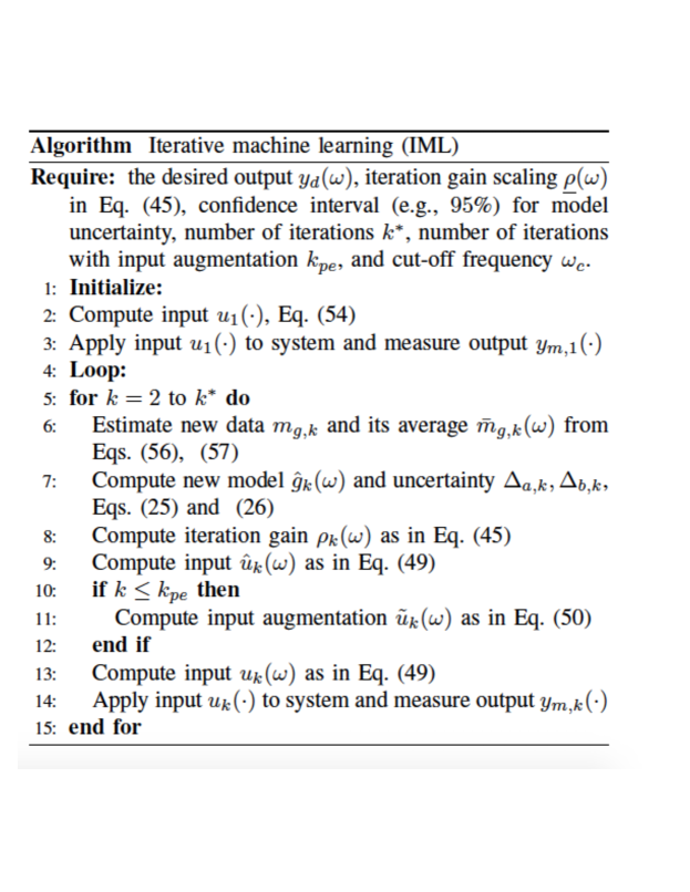
The proposed iterative machine learning (IML) algorithm using GPR is described below in Fig. 1

Figure 1: Iterative machine learning (IML)

5 Simulation results and discussion

Simulation results are presented on convergence of the trajectory tracking input with the proposed IML approach. The impact of using the additional input for persistency of excitation on the learning of the model is illustrated. Additionally, the advantage of using the model learning to improve tracking of a new trajectory is illustrated.

5.1 Example system

Consider a non-minimum phase example system $g(s)$ in Eq. (1) of the form

$$g(s)=\frac{-\frac{\omega_{p1}^{2}\omega_{p2}^{2}}{\omega_{z}^{2}}\left[(s-\omega_{z})(s+\omega_{z})\right]}{\left[s^{2}+2{\zeta_{p1}}{\omega}_{p1}s+\omega_{p1}^{2}\right]\left[s^{2}+2{\zeta_{p2}}{\omega_{p2}}s+\omega_{p2}^{2}\right]}.$$ (58)

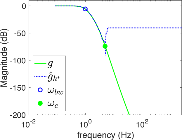
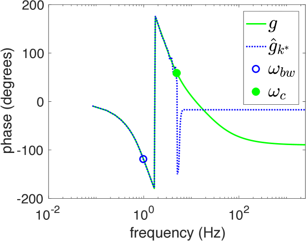
Let the larger pole frequency $\omega_{p2}=6\pi$ rads/s be three times the smaller pole frequency $\omega_{p1}=2\pi$ rads/s, with the zero $\omega_{z}=4\pi$ rads/s interlaced between the poles and the damping ratios as $\zeta_{p1}=\zeta_{p2}=1\sqrt{2}$. Note that the system has relative degree two (since the number of poles is two more than the number of zeros) and hence the desired output $y_{d}$ needs to be twice differentiable to enable exact tracking. The frequency response of the example system (with the above parameter values) is shown in Fig. 2. The system bandwidth is about one Hz, $\omega_{bw}\approx 1$ Hz. Since output tracking is not usually anticipated much beyond the system bandwidth (see Remark 10), the cutoff frequency $\omega_{c}$ for computing the model $\hat{g}$ and the iteration input $u_{k}$ is selected as $\omega_{c}=5$ Hz — about five times the system bandwidth $\omega_{bw}$.

Figure 2: Frequency response of the example system $g$ in Eq. (58): (top) magnitude; and (bottom) phase in degrees. The learned model $\hat{g}$ is also shown.

5.2 Desired trajectory

Consider a twice-differentiable, desired trajectory $y_{d}$, with zero initial position $y_{d}(0)=0$ and velocity $\dot{y}_{d}(0)=0$, and specified by its second time derivative $\ddot{y}_{d}$ as

$$\ddot{y}_{d}(t)=\left\{\begin{aligned} &\sum_{n=1}^{n=N}\sin[n\omega_{*}(t-t_{0})]&\quad&{\mbox{if}}~{}t_{0}<~{}t<t_{1}\\ &-\sum_{n=1}^{n=N}\sin[n\omega_{*}(t-t_{1})]&\quad&{\mbox{if}}~{}t_{1}<~{}t<t_{2}\\ &0&\quad&{\mbox{otherwise}},\end{aligned}\right.$$ (59)

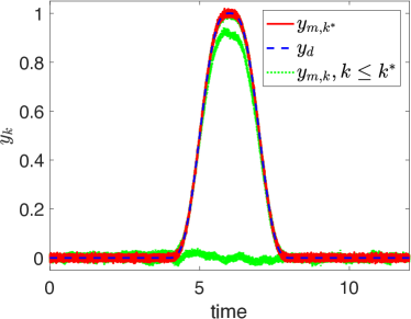
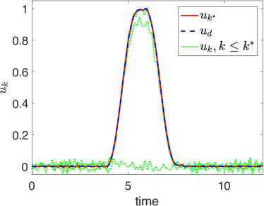
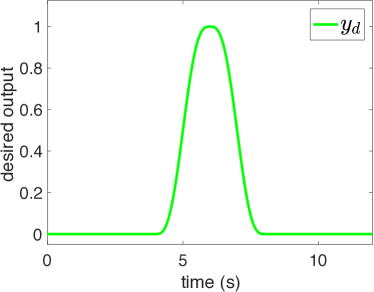
where main frequency component $\omega_{*}=0.5$ Hz that is about half the system bandwidth $\omega_{bw}$, the number of harmonics $N$ in the desired output $y_{d}$ was one, i.e., $N=1$ and $t_{0}=4$s, $t_{1}=6$s, $t_{2}=8$s. A plot of the desired output is shown in Fig. 3. The padding around the middle section $t\in[4,8]$ is added to enable noncausal solutions. The computations are performed in the time domain with a sampling time of $0.2$ms and in the discrete-frequency domain with the fast Fourier transform (FFT) using MATLAB.

5.3 Impact of additional input for persistency of excitation

The error in the model data from Eq. (56) can be large in the presence of noisy output measurements $y_{m,k}(\omega)$. To illustrate, the error in the model data are compared below, with and without the persistency of excitation, when the input $u(\omega)$ is the exact tracking input $u_{d}(\omega)$ from Eq. (2), for frequency $\omega$ less than the cutoff frequency $\omega_{c}$.

The standard deviation $\sigma_{n_{y}}(\omega)$ of the output noise $n_{y,d}(\omega)$ in the simulations is, similar to  (52),

$$\sigma_{n_{y}}~{}~{}=\sigma_{y,a}(\omega)~{}=\sigma_{y,b}(\omega)=\frac{1}{10^{4}}\max_{\omega\leq\omega_{c}}\left[{y}_{d}(\omega)\right]$$ (60)

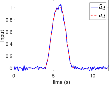
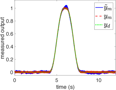
and the resulting input and output are shown in Fig. 3.

Figure 3: Comparison of input and output with and without persistency of excitation. Desired output (top left). Input $u$ (top right) : (case i) the inverse input $u_{d}$ for the desired output $y_{d}$ from Eq. (2); and (case ii) the augmented input $\tilde{u}_{d}$ from Eq. (64) with persistency of excitation. Resulting measured output $y_{m}$ from Eq. (61) and $\tilde{y}_{m}$ from Eq. (67) are shown in time domain (bottom left) and frequency domain (bottom right). The plot of the measured outputs $y_{m},\tilde{y}_{m}$ (bottom left) overlaps the plot of the desired output $y_{d}$.

5.3.1 Effect of measurement noise

The noisy measured output $y_{m}$, as in Eq. (52),

$$y_{m,d}(\omega)~{}=y_{d}(\omega)+n_{y,d}(\omega)~{}=g(\omega){u}_{d}(\omega)+n_{y,d}(\omega)$$ (61)

shown in Fig. 3 is close to the desired output $y_{d}$ with the inverse feedforward input $u=u_{d}$. With this measured output $y_{m,d}$, the model data can be computed from Eq. (56) as

$$m_{g}(\omega)~{}~{}={m}_{a}(\omega)+j{m}_{b}(\omega)~{}=\frac{y_{m,d}(\omega)}{u_{d}(\omega)}.$$ (62)

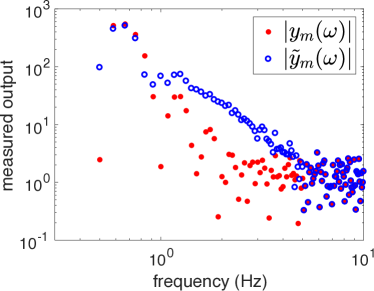
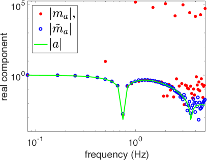
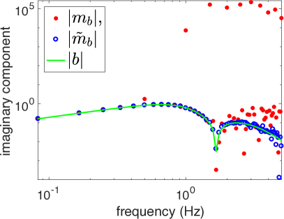
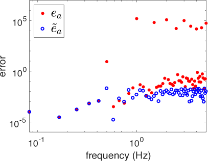
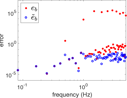
The error $e_{a},e_{b}$ in the model data components $m_{a},m_{b}$ increases with frequency since the output $y_{d}$ tends to become small compared to the output noise $\sigma_{n_{y}}$, e.g., at frequencies, $\omega>1$ Hz, as seen in Fig. 4 (bottom two plots). The maximum model-data error $e_{a,max},e_{b,max}$ in the real and imaginary components of the model data are

$$e_{a,max}{} =\max_{\omega\leq\omega_{c}}\left[e_{a}(\omega)={|m_{a}(\omega)-a(\omega)|}\right]~{}=1.58\times 10^{5}$$ (63)

$$e_{b,max}{} =\max_{\omega\leq\omega_{c}}\left[e_{b}(\omega)={|m_{b}(\omega)-b(\omega)|}\right]~{}=2.24\times 10^{5}.$$

Figure 4: Impact of persistency of excitation on acquired model data. Top two plots compare the absolute values of the real and imaginary components $a,b$ for the example system $g$ in Eq. (58) with the components of the data $m_{a},m_{b}$ from Eq. (62) and $\tilde{m}_{a},\tilde{m}_{b}$ from Eq. (68). The bottom two plots compare the model-data error for the two cases, $e_{a},e_{b}$ in Eq. (63) and $\tilde{e}_{a},\tilde{e}_{b}$ in Eq. (69).

5.3.2 Reduction of noise effect with persistency of excitation

To evaluate the advantage of persistency of excitation, consider the augmentation of the inverse input ${u}_{d}(\omega)$ to $\tilde{u}_{d}(\omega)$, as in Eq (50), at frequency $\omega$ less than the cutoff frequency $\omega_{c}$,

$$\tilde{u}_{d}(\omega)~{}=u_{d}(\omega)+\tilde{u}(\omega)e^{j[\phi_{d}(\omega)]}\\$$ (64)

whenever the input $u_{d}(\omega)$ was small,

$$|{u}_{d}(\omega)|<u_{pe}(\omega)=10\sigma_{n_{y}}$$ (65)

with the additional input magnitude and phase given by

$$\tilde{u}(\omega)~{}~{}=100\sigma_{n_{y}},\quad\phi_{d}(\omega)~{}\sim{\mathcal{N}}\left(0,\pi^{2}\right),\quad\omega\leq\omega_{c}.$$ (66)

The resulting augmented input $\tilde{u}_{d}$ and the associated measured output $\tilde{y}_{m,d}$ with the same noise $n_{y,d}(\omega)$ as the unaugmented case in Eq. (61)

$$\tilde{y}_{m,d}(\omega)~{}=g(\omega)\tilde{u}_{d}(\omega)+n_{y,d}(\omega)$$ (67)

are shown in Fig. 3. The effect of measurement noise in the model estimates from Eq. (56)

$$\tilde{m}_{g}(\omega)~{}~{}=\tilde{m}_{a}(\omega)+j\tilde{m}_{b}(\omega)~{}=\frac{\tilde{y}_{m,d}(\omega)}{\tilde{u}_{d}(\omega)}.$$ (68)

are shown in Fig. 4 (top two plots), which compares the real and imaginary components $a(\omega),b(\omega)$ of the example system $g(\omega)$ in Eq. (58) with the real and imaginary components of the model data estimated for the two cases: (case i) the inverse input $u_{d}(\omega)$ from Eq. (2) and (case ii) the input $\tilde{u}_{d}(\omega)$ with persistency of excitation from Eq. (64). Note that the model data with the persistency of excitation input $\tilde{u}_{d}(\omega)$ tend to be closer to the actual system $g(\omega)$ when compared to the case without the persistency of excitation as seen in Fig. 4. The maximum model-data error $\tilde{e}_{a,max},\tilde{e}_{b,max}$ in the real and imaginary components, with the persistency of excitation input, over all frequencies $\omega\leq\omega_{c}$, are

$$\tilde{e}_{a,max}{} =\max_{\omega\leq\omega_{c}}~{}\left[\tilde{e}_{a}(\omega)={|\tilde{m}_{a}(\omega)-a(\omega)|}\right]~{}=0.020,$$ (69)

$$\tilde{e}_{b,max}{} =\max_{\omega\leq\omega_{c}}~{}\left[\tilde{e}_{b}(\omega)={|\tilde{m}_{b}(\omega)-b(\omega)|}\right]~{}=0.027.$$

Thus, the addition the persistency of excitation input (with relatively-small change on the output, typically at high-frequency, as seen in Fig. 3) can lead to substantially smaller model error $\tilde{e}_{a,max},\tilde{e}_{b,max}$ in Eq. (69) than the model error $e_{a,max},e_{b,max}$ in Eq. (63) without the persistency of excitation — several orders of magnitude less error, as seen in Fig. 4, (bottom two plots).

5.4 Convergence with iterations

Convergence with the proposed IML approach is discussed below with the initial input $u_{1}$ chosen with the augmented input in Eq. (54) and without prior knowledge of the model, i.e., $\hat{u}_{1}(\omega)=0$ in Eq. (54).

5.4.1 GPR results

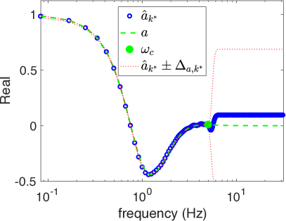
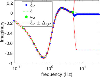
All available data ${m}_{g,i}(\omega)$ with $i=1,2,\ldots k$ is used to predict the model $\hat{g}_{k}$ using GPR with fitrgp and predict functions in MATLAB, where the covariance function is the squared exponential kernel, and the hyperparameters are optimized using the data. With the total number of iterations selected as $k^{*}=5$ and model augmentation during the first three iterations $k_{pe}=3$ in Eq. (50), the estimated the model data $\hat{g}_{k^{*}}(\omega)$ is close to the system $g(\omega)$ as seen in Fig. 5. The $95\%$ confidence intervals $\Delta_{a,k},\Delta_{b,k}$ (e.g., shown in Fig. 5 for the final iteration $k=k^{*}$) are used as the expected bounds on the model uncertainty as in Eq. (27).

Figure 5: Results of the Gaussian process regression. The fit from the GPR $\hat{a}_{k^{*}}(\omega),\hat{b}_{k^{*}}(\omega)$ is close to the system ${a}(\omega),{b}(\omega)$ — the fit overlaps the model upto the cutoff frequency $\omega_{c}$ due to the augmented input and deviations become noticeable beyond $\omega_{c}$. The 95% confidence interval (dotted lines) is small till the cutoff frequency $\omega_{c}$.

5.4.2 Selection of iteration gain

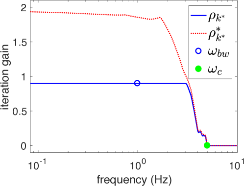
The iteration gain $\rho_{k}(\omega)$ was chosen as in Eq. (45) with $\underline{\rho}(\omega)=0.9$. The iteration gain $\rho_{k^{*}}(\omega)$ and its upper bound $\rho_{k^{*}}^{*}(\omega)$ from Eq. (41) at the final iteration step $k^{*}$ are shown in Fig. 6, which tends to zero at high frequency when the model size becomes small compared to the measurement noise, as in Remark 10.

Figure 6: The maximum possible iteration gain $\rho_{k^{*}}^{*}(\omega)$ from Eq. (41) and the selected iteration gain $\rho_{k^{*}}$ used to compute the final input $u_{k^{*}}(\omega)$.

Remark 14 (Cutoff frequency)

While the iteration gain $\rho(\omega)$ acts as a low-pass filter and tends to zero at high frequency $\omega$ when the system $g(\omega)$ tends to zero, e.g., see Fig. 6, the cutoff frequency $\omega_{c}$ (beyond which the iteration gain $\rho(\omega)$ is set to zero) is used to avoid potential divergence at high-frequencies where the model size and the allowable uncertainty are expected to be small.

5.4.3 Input and model convergence

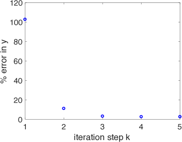
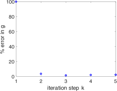
Convergence is achieved as the iteration steps $k$ increase, i.e., the model converges to the system response $\hat{g}_{k}(\omega)\rightarrow g(\omega)$ and the output converges to the desired output $y_{k}(\cdot)\rightarrow y_{d}(\cdot)$, as seen in Fig. 7. The modeling error $e_{g,k}$ given by

$$e_{g,k}{} =\frac{\max_{\omega\leq\omega_{c}}|\hat{g}_{k}(\omega)-g(\omega)|}{\max_{\omega\leq\omega_{c}}|g(\omega)|}\times 100,$$ (70)

reduced to $e_{g,k^{*}}=2.0$% at the final iteration $k=k^{*}$. The output tracking error $e_{y,k}$ given by

$$e_{y,k}{} =\frac{\max_{t}|y_{k}(t)-y_{d}(t)|}{\max_{t}|y_{d}(t)|}\times 100,$$ (71)

reduced to $e_{y,k^{*}}=2.48$% at the final iteration $k=k^{*}$, which is the same as the noise level, i.e.,

$$\frac{\max_{t}|n_{y,k^{*}}(t)|}{\max_{t}|y_{d}(t)|}\times 100=2.48.$$ (72)

Figure 7: (Top left) Convergence of the measured output $y_{m,k}$ to the desired output $y_{d}$. (Top right) Convergence of the input $u_{k}$ to the inverse feedforward input $u_{d}$ in Eq. (2). (Bottom left) Output tracking error $e_{y,k}$ from Eq. (71). (Bottom right) Modeling error $e_{g,k}$ from Eq. (70).

5.5 Impact of model learning for new output

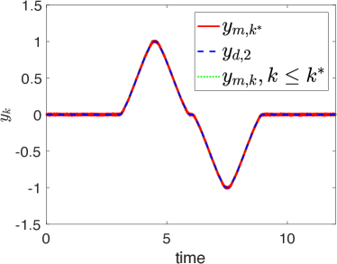
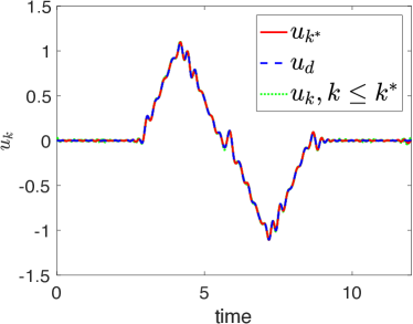
The impact of model learning for tracking was evaluated for a new desired output $y_{d,2}$ with a higher main frequency $\omega_{*}=2/3$ Hz compared to the previous desired output, and five harmonics $N=5$ in Eq. (59). A plot of the desired output is shown in Fig. 8. Even with this increase in the amplitude of the desired output at higher frequencies, the initial input $u_{1}$

$$u_{1}(\omega){} =\hat{g}_{1}^{-1}(\omega)\left[y_{d}(\omega)\right]~{}~{}\forall~{}\omega\leq\omega_{c},$$ (73)

found with the initial model $\hat{g}_{1}$ defined as the final model $\hat{g}_{k^{*}}$ from the previous iterations, led to good initial tracking as seen in Fig. 8. (The input augmentation was not added to this initial input to clarify the impact of using the model from the previous iterations.) The input augmentation was used for iteration steps $k=2,k=3$ and the total number of iterations was $k^{*}=5$. The output tracking error (with five iterations) is small — the measured outputs $y_{m,k}$ for all five iterations tend to overlap the desired output $y_{d,2}$ in Fig. 8. The initial tracking error $e_{y,1}$ for the new output trajectory $y_{d,2}$ at the first iteration step was $2.97$%, which is close to the noise level of $2.12$% — the tracking error $e_{y,5}$ at the end of five iterations for the second output $y_{d,2}$ is $2.15$%. Thus, as expected, the learning of the model during the iteration process with the previous desired output trajectory $y_{d}$ leads to small initial error in the iterations when learning the new desired output $y_{d,2}$. In this sense, the propose IML improves the performance and portability of the frequency-domain iterative control.

Figure 8: Iteration results for new desired output $y_{d,2}$ for five iterations, $k^{*}=5$. (Left) All five measured outputs $y_{m,k}$ ($k=1,\ldots 5$) overlap the desired output $y_{d,2}$. (Right) All five computed inputs $u_{k}$ are close to the inverse feedforward input $u_{d}$ in Eq. (2) and have substantial higher frequency content when compared to the input for the initial output trajectory $y_{d}$ in Fig. 7.

6 Conclusions

This article proposed a frequency-domain iterative machine learning (IML) approach to simultaneously update the system model while learning the inverse input. Additionally, inputs with persistency of excitation were proposed to promote learning of the model by generating data at frequencies outside the main frequency content of the specified desired output. The method was applied to a simulation example, and results show the model learning can substantially reduce the initial error for other desired output trajectories.

7 Acknowledgment

This work was partially supported by NSF grant CMII 1536306 and the Helen R. Whiteley Center at Friday Harbor.

References

- [1] S. Arimoto, S. Kawamura, and F. Miyazaki. Bettering operation of robots by learning. J. of Robotic Systems, 1(2):123–140, March 1984.
- [2] J. J. Craig. Adaptive control of manipulators through repeated trials. Proceedings of the American Control Conference, page 1566 1573, 1984.
- [3] C. G. Atkeson and J. McIntyre. Robot trajectory learning through practice. In IEEE Int. Conf. on Robotics and Automation, pages 1737–1742, 1986.
- [4] Yang Li and John Bechhoefer. Feedforward control of a piezoelectric flexure stage for AFM. Proceedings of American Control Conference, Seattle, WA, pages 2703–2709, June 11-13, 2008.
- [5] G. M. Clayton and S. Devasia. Iterative image-based modeling and control for higher scanning probe microscope performance. Review of Scientific Instruments, 78(8):Article No. 083704 (pp. 1–12), August 29, 2007.
- [6] G. Schitter, R. W. Stark, and A. Stemmer. Fast contact-mode atomic force microscopy on biological specimen by model-based control. Ultramicroscopy, 100(3-4):253–257, Aug, 2004.
- [7] K.-S. Kim and Q. Zou. Model-less inversion-based iterative control for output tracking: Piezo actuator example. Proceedings of American Control Conference, Seattle, WA, pages 2170–2715, June 11-13, 2008.
- [8] K. K. Leang and S. Devasia. Design of hysteresis-compensating iterative learning control: Application to atomic force microscopes. Mechatronics, 16(3-4):141–158, April-May, 2006.
- [9] Ying Wu and Qingze Zou. Iterative control approach to compensate for both the hysteresis and the dynamics effects of piezo actuators. IEEE Transactions on Control Systems Technology, 15(5):936–944, September, 2007.
- [10] M. P. Chaffe and L. Y. Pao. Iterative learning control for near-field scanning optical microscope applications. In 2011 IEEE International Conference on Control Applications (CCA), pages 1075–1080, Sept 2011.
- [11] Stan H. van der Meulen, Rob L. Tousain, and Okko H. Bosgra. Fixed Structure Feedforward Controller Design Exploiting Iterative Trials: Application to a Wafer Stage and a Desktop Printer. ASME. J. Dyn. Sys., Meas., Control, 130(7):051006–051006 1–16, Sept 2008.
- [12] Joost Bolder and Tom Oomen. Rational Basis Functions in Iterative Learning Control-With Experimental Verification on a Motion System. IEEE Transactions on Controls Systems Technology, 23(2):722–729, MAR 2015.
- [13] S. Mishra and M.Tomizuka. Segmented iterative learning control for precision positioning of waferstages. In 2007 IEEE/ASME international conference on advanced intelligent mechatronics AIM, pages 1–6, Sept 2007.
- [14] D. Gorinevsky, D. E. Torfs, and A. A. Goldenberg. Learning approximation of feedforward control dependence on the task parameters with application to direct-drive manipulator tracking. IEEE Transactions on Robotics and Automation, 13(4):567–581, Aug 1997.
- [15] K. L. Moore. Iterative Learning Control for Deterministic Systems. Springer-Verlag, London, U.K., 1993.
- [16] S. Tien, Qingze Zou, and S. Devasia. Control of dynamics-coupling effects in piezo-actuator for high-speed afm operation. In Proceedings of the 2004 American Control Conference, volume 4, pages 3116–3121 vol.4, June 2004.
- [17] J. Hatonen, T.J. Harte, D.H. Owens, J. Ratcliffe, P. Lewin, and E. Rogers. Iterative learning control - what is it all about? {IFAC} Proceedings Volumes, 37(12):547 – 553, 2004. {IFAC} Workshop on Adaptation and Learning in Control and Signal Processing (ALCOSP 04) and {IFAC} Workshop on Periodic Control Systems (PSYCO 04), Yokohama, Japan, 30 August - 1 September, 2004.
- [18] S. Tien, Q. Zou, and S. Devasia. Iterative control of dynamics-coupling-caused errors in piezoscanners during high-speed AFM operation. IEEE Transactions on Control Systems Technology, 13(6):921–931, Nov 2005.
- [19] H.-S. Ahn, Y. Q. Chen, and K. L. Moore. Iterative learning control: Brief survey and categorization. IEEE Transactions on Systems, Man, and Cybernetics, Part C: Applications and Reviews, 37(6):1099–1121, 2007.
- [20] J. Ghosh and B. Paden. Iterative learning control for nonlinear nonminimum phase plants. ASME Journal of Dynamic Systems, Measurement, and Control, 123:21–20, March,2001.
- [21] D.A. Bristow and A.G. Alleyne. Monotonic convergence of iterative learning control for uncertain systems using a time-varying filter. IEEE Transactions on Automatic Control, 53(2):582 – 585, March, 2008.
- [22] J. Ghosh and B. Paden. A pseudo-inverse based iterative learning control. IEEE Trans. on Automatic Control, 47(5):831–837, May,2002.
- [23] C. Peng, L. Sun, W. Zhang, and M. Tomizuka. Optimization-based constrained iterative learning control with application to building temperature control systems. In 2016 IEEE International Conference on Advanced Intelligent Mechatronics (AIM), pages 709–715, July 2016.
- [24] Bing Chu, David H. Owens, and Christopher T. Freeman. Iterative Learning Control With Predictive Trial Information: Convergence, Robustness, and Experimental Verification. IEEE Transactions on Controls Systems Technology, 24(3):1101–1108, MAY 2016.
- [25] M. Norrlof. An adaptive iterative learning control algorithm with experiments on an industrial robot. IEEE Transactions on Robotics and Automation, 18(2):245–251, Apr 2002.
- [26] Mark Butcher, Alireza Karimi, and Roland Longchamp. Iterative learning control based on stochastic approximation. In 17th IFAC World Congress, Seoul, Korea, July 6-11 2008.
- [27] X. Gao and S. Mishra. An iterative learning control algorithm for portability between trajectories. In 2014 American Control Conference, Portland, OR, pages 3808–3813, June 4-6 June, 2014.
- [28] Joost Bolder, Tom Oomen, Sjirk Koekebakker, and Maarten Steinbuch. Using iterative learning control with basis functions to compensate medium deformation in a wide-format inkjet printer. MECHATRONICS, 24(8):944–953, DEC 2014.
- [29] J. van Zundert, J. Bolder, and T. Oomen. Iterative learning control for varying tasks: Achieving optimality for rational basis functions. In 2015 American Control Conference (ACC), pages 3570–3575, July 2015.
- [30] C. T. Freeman, P. L. Lewin, E. Rogers, D. H. Owens, and J. J. Hatonen. Discrete fourier transform based iterative learning control design for linear plants with experimental verification. ASME Journal of Dynamic Systems, Measurement, and Control, 131(3):031006–1 – 031006–10, May,2009.
- [31] K.-S. Kim and Q. Zou. A modeling-free inversion-based iterative feedforward control for precision output tracking of linear time-invariant systems. IEEE/ASME Transactions on Mechatronics, 18(6):1767–1777, Dec. 2013.
- [32] W. Wang and Q. Zou. A modeling-free differential-inversion-based iterative control approach to simultaneous hysteresis-dynamics compensation: high-speed large-range motion tracking example. American Control Conference, Palmer House Hilton, Chicago, IL, USA, July 1-3 2015.
- [33] C. E. Rasmussen and C. K. I. Williams. Gaussian Processes for Machine Learning. The MIT Press, Cambridge, MA, 2006.
- [34] K. J. Astrom and B. Wittenman. Adaptive Control. Addison Wesley, New York, 1989.
- [35] Gianluigi Pillonetto, Francesco Dinuzzo, Tianshi Chen, Giuseppe De Nicolao, and Lennart Ljung. Kernel methods in system identification, machine learning and function estimation: A survey. Automatica, 50(3):657 – 682, 2014.
- [36] R. Boloix-Tortosa, F. J. Pay n-Somet, E. Arias de Reyna, and J. J. Murillo-Fuentes. Complex kernels for proper complex-valued signals: A review. In 2015 23rd European Signal Processing Conference (EUSIPCO), pages 2371–2375, Aug 2015.
- [37] P. M. Sammons, D. A. Bristow, and R. G. Landers. Iterative learning control of bead morphology in laser metal deposition processes. In 2013 American Control Conference, pages 5942–5947, June 2013.
- [38] David J. Hoelzle and Kira L. Barton. On Spatial Iterative Learning Control via 2-D Convolution: Stability Analysis and Computational Efficiency. IEEE Transactions on Controls Systems Technology, 24(4):1504–1512, JUL 2016.
- [39] Nanjun Liu and Andrew Alleyne. Iterative Learning Identification for Linear Time-Varying Systems. IEEE Transactions on Controls Systems Technology, 24(1):310–317, JAN 2016.
- [40] S. Devasia. Should model-based inverse inputs be used as feedforward under plant uncertainty? IEEE Transactions on Automatic Control, 47(11):1865–1871, Nov, 2002.
- [41] F. Perez-Cruz, J. J. Murillo-Fuentes, and S. Caro. Nonlinear channel equalization with gaussian processes for regression. IEEE Transactions on Signal Processing, 56(10):5283–5286, Oct 2008.
- [42] John Bechhoefer. Kramers- Kronig, Bode, and the meaning of zero. American Journal of Physics, 79(10):1053–1059, 2011.