Comparing the Finite-Time Performance of Simulation-Optimization Algorithms

ABSTRACT

We empirically evaluate the finite-time performance of several simulation-optimization algorithms on a testbed of problems with the goal of motivating further development of algorithms with strong finite-time performance. We investigate if the observed performance of the algorithms can be explained by properties of the problems, e.g., the number of decision variables, the topology of the objective function, or the magnitude of the simulation error.

1 INTRODUCTION

The practice of simulation optimization (SO) deals with optimizing a real-valued objective function that cannot be evaluated exactly, but instead must be estimated via simulation. In addition to the challenge of estimating the objective function, structural properties of the objective function, e.g., continuity, differentiability, or convexity, may be unknown. On account of this, SO algorithms are often designed to solve a broad class of problems without exploiting any structure of the objective function.

In the SO literature, one commonly sees theoretical results on the asymptotic performance of an algorithm. It is often shown that an algorithm will converge to a local or global optimizer as the simulation effort approaches infinity. Some results further specify a rate at which an algorithm converges once within a neighborhood of an optimizer. Unfortunately, the asymptotic regimes in which these results hold likely require an amount of computational effort that exceeds practical budgets, making the asymptotic results less useful to practitioners. For a practitioner deciding which algorithm to use for a particular problem, understanding the finite-time performance of an algorithm is more meaningful.

The SO community lags behind other research communities when it comes to having an established testbed of problems and developing metrics for comparing the finite-time performance of algorithms [8]. Moreover, a comprehensive comparison of SO algorithms has not been done on a large testbed [1]. As a first step toward such a comparison, we implement several popular SO algorithms and test them on a subset of problems from SimOpt (SimOpt Library [10]), a growing library of SO problems developed by Pasupathy and Henderson [9]. We evaluate the finite-time performance of the algorithms and discuss insights into the types of problems on which the algorithms might be expected to perform well. An objective of our study is to spur the development of SO algorithms that have strong finite-time performance for various classes of problems. We also hope to encourage further contributions to the SimOpt library so that a more comprehensive testbed of SO problems is available to researchers for evaluating new algorithms.

2 EVALUATING FINITE-TIME PERFORMANCE

In deterministic optimization, an algorithm’s performance on a given problem is usually measured by either the number of function evaluations or the wall-clock time needed to find the optimal solution or to get within a specified tolerance. In this way, one can easily compare algorithms. Applying this approach to SO algorithms runs into several challenges. Firstly, the optimal solutions to SO problems are often unknown or have no certificate of optimality. Secondly, sampling error makes it harder to determine whether the objective function value of a solution is within a given tolerance of the optimal objective function value. Instead, SO algorithms can be more fairly compared by fixing a given simulation budget—either the wall-clock time or the number of objective function evaluations—and evaluating the objective function at the estimated best solution visited within the budget.

Although measuring a computational budget in terms of wall-clock time may make sense from a practical standpoint, the resulting performances are platform dependent. On the other hand, using the number of objective function evaluations as a measure of time has its own issues; see also Pasupathy and Henderson [8]. Firstly, a potentially significant portion of computation effort may go unmeasured if, for example, the constraints are stochastic or gradient information is calculated without taking additional objective function valuations. Secondly, for steady-state simulations that involve simulating a single, long sample path, counting one replication as one objective function evaluation may be misleading.

In our experiments, we specify the simulation budget in terms of the number of objective function evaluations. All of the problems we study have deterministic constraints and the simulations all have finite horizons. Moreover, we count all objective function evaluations towards the budget, including function evaluations used to obtain gradient estimates, e.g., via finite differences; see also Sect. 3.1.

For one macroreplication of an algorithm, let $Z(n)$ denote the true objective function value of the estimated best solution visited in the first $n$ objective function evaluations. Because the estimated best solution $X(n)$ is random, $Z(n)$ is a random variable. Conditional on the solution $X(n)$, the objective value $Z(n)$ is not random, but we probably cannot compute it exactly because we use simulation to evaluate the objective function. In our experiments, we get fairly precise estimates of $Z(n)$—conditional on $X(n)$—by running additional simulations in a post-processing step. These replications are not counted towards the algorithm’s budget. Plotting $Z(n)$ as a function of $n$ shows how the objective value of the estimated best solution changes as the algorithm progresses [8]. The $Z(n)$ curve has upward or downward jumps whenever a new solution is discovered that is believed to be the best.

Plotting the $Z(n)$ curve for a single macroreplication has limited value since the location of the curve is itself random. Instead, it is more informative to run several macroreplications of an algorithm and aggregate the results. In our experiments, we plot the mean performance curve $\bar{Z}(n):=m^{-1}\sum_{i=1}^{m}Z_{i}(n)$ for all $n$ where $Z_{i}(n)$ is the performance associated with the $i$th of $m$ macroreplications. An argument can also be made for considering the median performance of an algorithm as it is less sensitive to outliers in performance. The empirical cumulative distribution function (cdf) of $Z(n)$ also contains a great deal of information about how an algorithm performs, including its variability. Although plotting the empirical cdf of $Z(n)$ for a single algorithm on a single problem is straightforward, comparing empirical cdfs for multiple algorithms is challenging.

By testing algorithms on only a modest number of SO problems, we were able to present in this paper many of the plots of $\bar{Z}(n)$. Ideally, we would like to graphically compare the performances of algorithms across a large number of problems as is done in the deterministic optimization community using performance profiles [5]. Adapting performance profiles to simulation optimization remains an active area of research with a notable challenge being how exactly to define the performance ratio. We believe that performance profiles have great potential for future comparisons of SO algorithms, especially when a large testbed of problems is available.

3 ALGORITHMS AND PROBLEMS

3.1 Algorithms

We suppose that when evaluating a solution $x$, an algorithm observes $y(x)=f(x)+\varepsilon(x)$ where $f(x)$ is the value of the objective function $f$ at $x$ and $\varepsilon(x)$ is the observational noise associated with simulating $x$. We further assume that $\varepsilon(x)$ has a mean of zero and finite variance. In our implementations, each of the algorithms take 30 samples of a given solution to estimate its objective value.

All problems specify a deterministic domain $\mathcal{D}\subseteq\mathbb{R}^{d}$ where $d$ is the number of decision variables. Unless otherwise stated, the starting solution $x_{1}$ is drawn from within ${\cal D}$ according to some probability distribution. When the domain was bounded, we used a uniform distribution over ${\cal D}$ and when the domain was unbounded, we used either independent exponential or Laplace distributions for generating the components of $x_{1}$. In the case that an algorithm decides to simulate a solution $x_{k+1}\notin{\cal D}$, we move it to the boundary of ${\cal D}$ on the line connecting $x_{k+1}$ and the previous solution $x_{k}$.

For our experiments, we selected a variety of well-known SO algorithms and compared them with two baseline methods: random search and gradient-based search. We provide a high-level description of the algorithms here and refer the interested reader to our public repository (Bitbucket [3]) for the codes.

Random Search

Random search (RandomSearch) iteratively evaluates solutions that are drawn from $\cal D$ according to some fixed probability distribution until the simulation budget is exhausted.

Gradient Search with Random Restarts

The gradient-based search algorithm (GradSearch) approximates the gradient of the objective function at a given solution $x_{k}$ via $d$ finite differences. That is, the $j$th component of the approximation $\hat{g}(x_{k})$ is

$$\hat{g}_{j}(x_{k})=\frac{y(x_{k}+h_{j}e_{j})-y(x_{k}-h_{j}e_{j})}{2h_{j}},$$

where for iterations $k\geq 2$, $h_{j}:=\sqrt{\mathrm{Var}(y(x_{1}))}/(\sqrt{2r}\cdot\hat{g}_{j}(x_{1}))$, $\mathrm{Var}(y(x_{1}))$ is the estimated variance of the noise $\varepsilon(x_{1})$, $r$ is the number of replications taken at $x_{1}$, and $e_{j}$ is the $d$-dimensional unit vector whose $j$th entry is one. In the first iteration, we randomly draw two solutions $x_{1}$ and $x^{\prime}$ from $\mathcal{D}$ and set $h_{j}=\min_{i}\|x_{1}[i]-x^{\prime}[i]\|/3$ for all $j\in\{1,\ldots,d\}$, in order to compute $\hat{g}_{j}(x_{1})$. In a given iteration $k$, we first test a step size of $c_{k}=2$ by evaluating $y(x_{k}+\hat{g}_{k}\cdot c_{k})$ (for maximization problems). If this yields a better solution than $x_{k}$, we set $x_{k+1}=x_{k}+\hat{g}_{k}\cdot c_{k}$. Otherwise we iteratively divide $c_{k}$ by $2$ and test again, until either a better solution is found or $c_{k}$ is too small, in which case we choose $x_{k+1}$ to be a random point.

In order to prevent GradSearch from becoming trapped at a local optimum, the algorithm restarts from a randomly chosen solution if all of the following conditions are met:

• $y(x_{k})-y(x_{k+1})<\tau\cdot(1+\|y(x_{k+1})\|)$,    ii) $\quad\|x_{k}-x_{k+1}\|<\sqrt{\tau}\cdot(1+\|x_{k+1}\|)$,

• $\|\hat{g}_{k}\|<\sqrt[3]{\tau}\cdot(1+\|y(x_{k+1})\|)$, and    iv) $\quad\|\hat{g}_{k}\|<\mathrm{Var}(y(x_{k}))$,

where $\tau$ is a constant chosen by the user. In our experiments, we set $\tau=10^{-4}$.

The Simultaneous Perturbation Method

The Simultaneous Perturbation Method (SPSA) [11, 12] also performs an iterative search that starts from a randomly selected solution $x_{1}$ and approximates the gradient in each step. However, instead of using the method of finite differences, SPSA relies on a simultaneous perturbation approximation of the gradient: the $j$th component of $g(x_{k})$ is approximated as

$$\hat{g}_{j}(x_{k})=\frac{y(x_{k}+c_{k}\Delta_{k})-y(x_{k}-c_{k}\Delta_{k})}{2c_{k}\Delta_{k}(j)},$$

where $\Delta_{k}$ is a carefully chosen $d$-dimensional random vector; see Spall [12] for details. SPSA requires only two function evaluations per iteration to approximate the gradient, whereas GradSearch requires $2d$. For the step-length sequence, we used the “automatic gain selection” implementation of Spall [13].

The Stochastic Trust-Region Response-Surface Method

The Stochastic Trust-Region Response-Surface Method (STRONG) of Chang et al. [4] approximates the unknown objective function by a series of local models, where each model is sufficiently accurate within its corresponding trust region. In iteration $k$, STRONG constructs a local model $r_{k}$ that is believed to resemble the objective function within a trust region ${\cal B}(x_{k},\Delta_{k})$ of radius $\Delta_{k}$ centered at $x_{k}$. It then computes a point $x^{\ast}_{k}\in{\cal B}(x_{k},\Delta_{k})$ that is “close” to the optimum of $r_{k}$ over ${\cal B}(x_{k},\Delta_{k})$. The point $x^{\ast}_{k}$ is accepted and becomes the center point $x_{k+1}$ for the next iteration if the following two tests are both passed:

1. The improvement in objective value $y(x_{k})-y(x^{\ast}_{k})$ (for minimization problems and estimated by sampling) is sufficiently large compared to the predicted improvement $r_{k}(x_{k})-r_{k}(x^{\ast}_{k})$.

2. The improvement in objective value is statistically significant, accounting for observational noise.

If the local model fits the observed data at $x_{k}$ and $x^{\ast}_{k}$ well—indicated by satisfactory results to the above tests—then the radius of the trust region for the next iteration is increased. Otherwise it stays the same or, in the case of a poor prediction, is decreased.

Our implementation of STRONG follows Chang et al. [4], with the exception that we do not apply design of experiments to select the evaluation points for fitting. Instead, we use central finite differences to estimate the gradient and a BFGS update to estimate the Hessian. We also tested a version (STRONGstg1) that does not fit second-order models, i.e., it only applies the first stage of STRONG.

The Nelder-Mead Algorithm

The algorithm of Nelder and Mead [7] (Nelder-Mead) iteratively maintains a simplex of $d+1$ vertices whose centroid is denoted by $x_{k}$. In iteration $k$, the vertex with the worst observed objective value, say $z_{k}$, is reflected through the centroid of the remaining $d$ vertices to obtain a new point $z_{k}^{\prime}$ that is then sampled. If the observed value $y(z_{k}^{\prime})$ is worse than the values previously observed at the remaining $d$ vertices of the simplex, the simplex is contracted and $z_{k}^{\prime}$ is chosen closer to the centroid. Otherwise $z_{k}$ is removed from the simplex and $z_{k}^{\prime}$ is added as $(d+1)$st vertex. We implemented the improvements suggested by Barton and Ivey Jr. [2] for accelerating the convergence of the algorithm when function evaluations are noisy.

3.2 Benchmark Problems

We have compiled a testbed of 15 problems: 12 were taken from SimOpt and the other three (POMDPController, RoutePrices, and TollNetwork) were developed during the course of this project and will be made available on SimOpt upon publication. The characteristics of the problems are summarized in Table 1.

Table 1: The benchmark problems and their characteristics: The first column gives the abbreviations used in this paper and hyperlinks to their respective entries on SimOpt.

Problems	Name on SimOpt	Dimension	Optimal Solution
Ambulance	Ambulances in a Square	6	Unknown
CtsNews	Continuous Newsvendor	1	Known
DualSourcing	Dual Sourcing	2	Unknown
EOQ	Economic-Order-Quantity	1	Known
FacilityLocation	Facility Location	4	Unknown
MM1	M/M/1 Metamodel	3	Known
MultiModal	A Multimodal Function	2	Known
ParameterEstimation	Parameter Estimation: 2D Gamma	2	Known
POMDPController	Optimal Controller for a POMDP	10	Unknown
ProductionLine	Optimization of a Production Line	3	Unknown
QueueGG1	GI/G/1 Queue	1	Unknown
Rosenbrock	Rosenbrock’s Function	40	Known
RoutePrices	Route Prices for Mobility-on-Demand	12	Unknown
SAN	SAN Duration	13	Unknown
TollNetwork	Toll Road Improvements	12	Unknown

4 RESULTS AND DISCUSSION

For every problem, we ran 30 macroreplications of each algorithm. Each macroreplication produced a sequence of estimated best solutions $X(n)$, where $n$ ranges over the replication budget as specified by the problem’s description on SimOpt. As a post-processing step, we averaged 30 replications at each solution $X(n)$ to obtain estimates of the objective function $Z(n)$. These post-processing replications were independent of those used to identify the sequence of solutions $X(\cdot)$, and they use common random numbers across all algorithms. We then averaged the 30 estimates of $Z(n)$ to produce the $\bar{Z}(n)$ curve. Since SPSA uses the replication budget $N$ as an input, we reran the algorithm with different values of $N$ to produce each point of the $\bar{Z}(n)$ curve. We also calculated 95% normal confidence intervals around $\bar{Z}(n)$. In some instances, we show plots of the median performance and the first and third quartiles of the 30 (macroreplication) samples of $Z(n)$. We organize our discussion into groupings of problems with similar patterns in their $\bar{Z}(n)$ plots.

CtsNews, MM1, ParameterEstimation, and QueueGG1

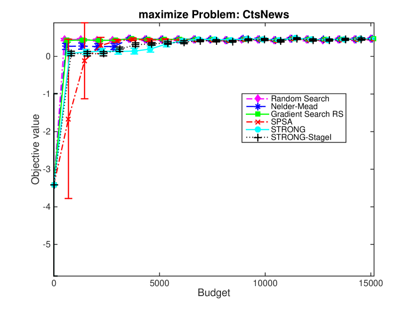
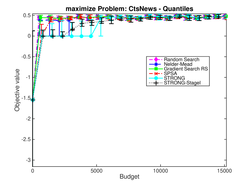
All algorithms work well on these low-dimensional problems, quickly converging to good solutions as illustrated in Figure 1 for the problem CtsNews. The plotted quantiles show that the performances of Nelder-Mead and STRONGstg1 are initially more variable than is suggested by the confidence intervals. We also see that SPSA’s performance has a large variance for small budgets, as reflected in the width of the confidence intervals. The high variance is not seen in the corresponding quantile plot, suggesting that SPSA has occasional very poor performance that shows up only in the below-0.25 quantiles (the worst quarter of the macroreplications).

Figure 1: CtsNews: (l) Average Performance, (r) Performance Quantiles

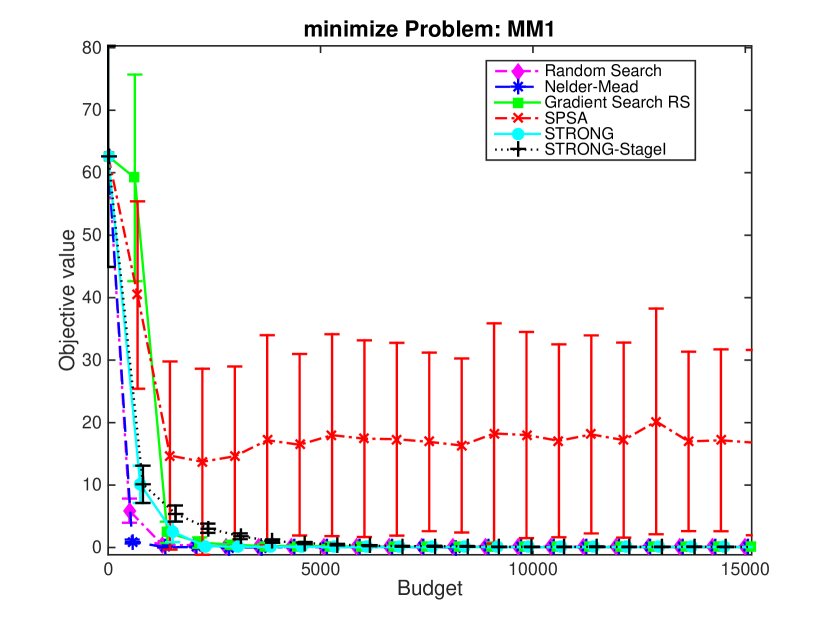
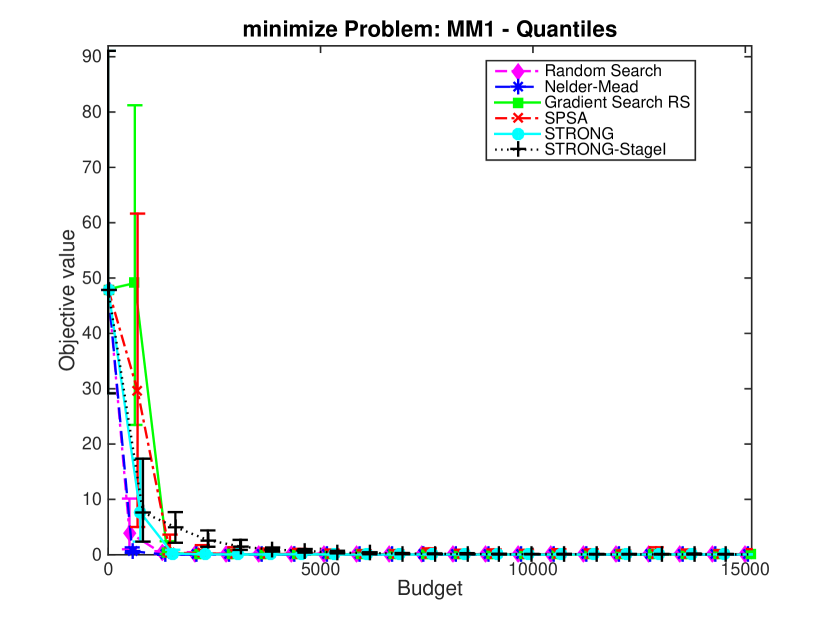
For the problem MM1, we noticed that the performance of SPSA was highly variable and worse than those of the other algorithms, as shown in Figure 2. However, the median performance of SPSA is competitive with those of the other algorithms. SPSA may be sensitive to the initial solution and occasionally can fail to make progress. This aspect of SPSA’s performance appeared in other problems; see the discussion of POMDPController.

Figure 2: MM1: (l) Average Performance, (r) Performance Quantiles

EOQ, DualSourcing

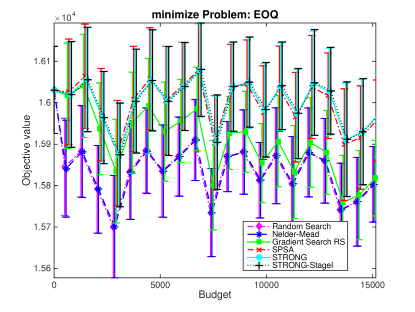
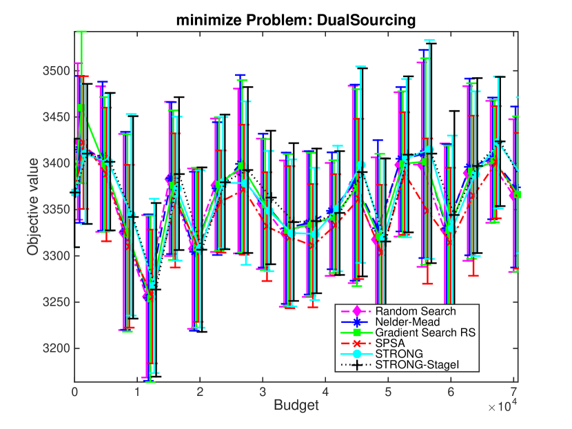
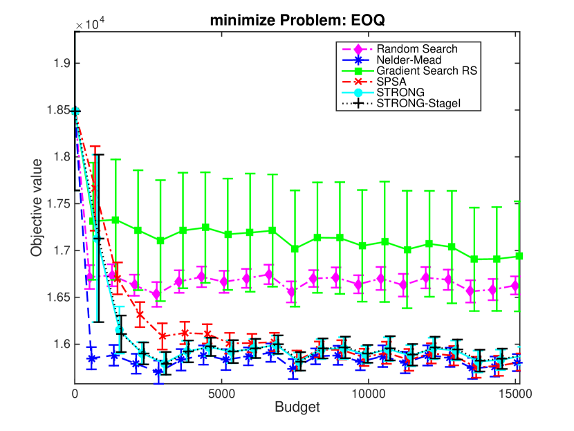
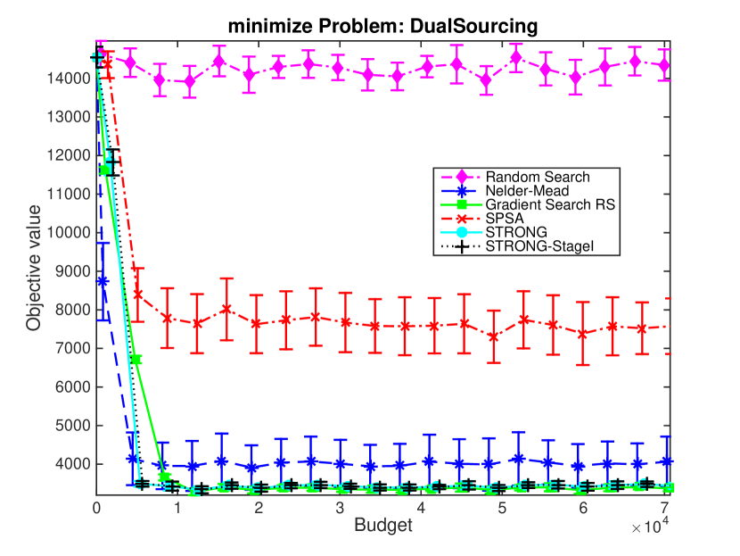
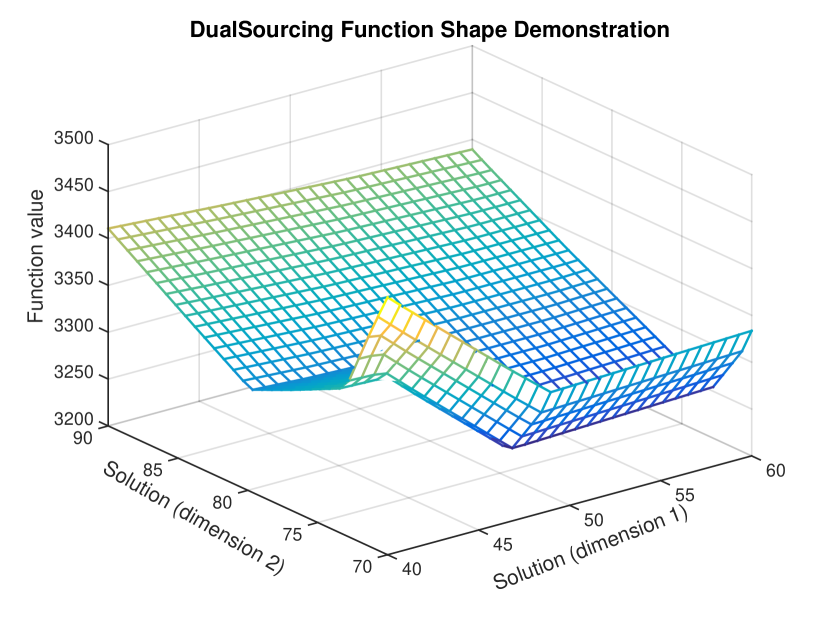
Our preliminary results for the problems EOQ and Dual Sourcing indicated that all of the algorithms had similar performance, quickly finding good solutions and then not improving further, as shown in Figure 3. We determined that the generated initial solutions were already near optimal for these two problems, as seen in the vertical scales on those plots. To induce differences in the performances across algorithms, we reran the algorithms, intentionally generating poor initial solutions; see Figures 4 and 5.

Figure 3: (l) EOQ: Average Performance, (r) DualSourcing: Average Performance

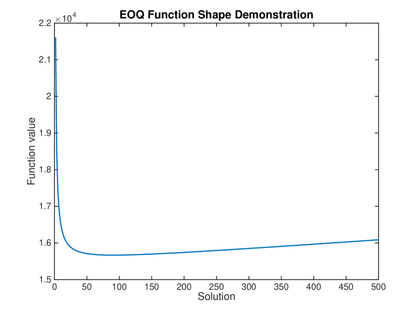
In Figure 4, all algorithms except GradSearch perform better than RandomSearch. GradSearch appears to fail due to the shape of the objective function—the function slope is steep to the left of the minimum but very flat to the right. Thus, when starting from a relatively small initial solution, the algorithm can first take a large step to a solution in the flat-slope area. Afterwards, GradSearch takes very small steps back towards the optimal solution. The performance of RandomSearch is highly dependent on the sampling distribution, which in these examples is not well calibrated, leading to poor performance.

Figure 4: EOQ: (l) Average Performance w/ Bad Initial Solutions, (r) The Objective function

For the problem DualSourcing (Figure 5), the extremely bad performance of RandomSearch can again be explained by the poorly-claibrated distribution for generating solutions. SPSA performs particularly poorly. The relatively weak performance of Nelder-Mead on this problem is the result of a few macroreplications on which the algorithm failed to find the optimal solution.

Figure 5: DualSourcing: (l) Average Performance w/ Bad Init., (r) Meshplot of the Objective Function

MultiModal, POMDPController, Rosenbrock, Toll Network

For these problems, most algorithms make rapid early progress and then stagnate.

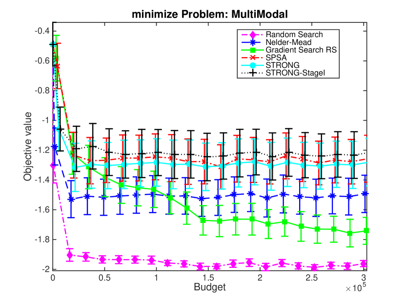
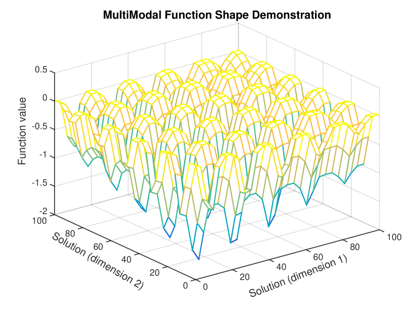
MultiModal is a 2-dimensional problem with 25 widely spaced local optima (Figure 6). Therefore, the local-search algorithms quickly improve on the initial solution, but then fail to make further progress. Meanwhile, the algorithms with restart, namely RandomSearch and GradSearch, manage to identify better solutions. Compared to RandomSearch, GradSearch is less efficient because it only employs random restarts once it fails to make progress, so it has fewer opportunities to restart. It only finds the global optimum around half of the time, which helps to explain the high variance of its performance in the results.

Figure 6: Multimodal: (l) Average Performance, (r) Meshplot of the Objective Function

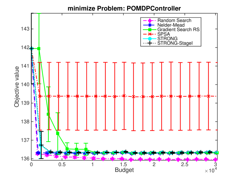
We observed that the problem POMDPController was hard for most algorithms to solve (see Figure 7). A plot of the objective function for the case $d=2$ shows that the objective function is made up of two plateaus with a narrow valley running through one of the plateaus. The optimal solution is at the bottom of the valley. The valley is hard to find because it is such a small region in the domain. In higher dimensions, such as the case $d=10$ that we tested, it is likely that good solutions are located in an even smaller region of the domain. In addition, gradient-based methods struggle because estimates of the gradient on the plateaus are close to zero and therefore dominated by noise. This helps explain why RandomSearch outperforms the other methods. The mean performance of SPSA is dominated by a few macroreplications on which it performed very poorly, perhaps because it produces very noisy gradient estimates that are based on only two objective function evaluations.

Figure 7: (l) POMDPController: Average Performance, (r) Rosenbrock: Average Performance

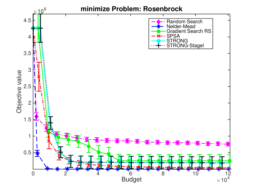
The Rosenbrock problem has the highest dimension of all our problems. As expected, RandomSearch performs poorly in searching a high-dimensional space (Figure 7). Nelder-Mead performs exceptionally well. Occasionally, GradSearch reaches the boundary of the feasible region and the estimated gradient indicates a search direction outside the boundary. We do not use a projected-gradient algorithm, instead simply pinning solutions back to the boundary, so GradSearch can stall on this problem. The two trust-region algorithms appear to struggle, perhaps for the same reason that GradSearch struggles. As expected, SPSA performs very well in this high-dimensional problem, owing to its cheap gradient estimates.

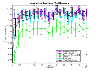
For the TollNetwork problem, GradSearch struggled relative to the other algorithms (Figure 8). We do not have an explanation for why GradSearch performs so poorly on this problem.

Figure 8: TollNetwork: Average Performance

Ambulance, FacilityLocation, ProductionLine, RoutePrices, SAN

The algorithms have highly varied performance on these five problems.

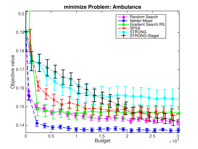
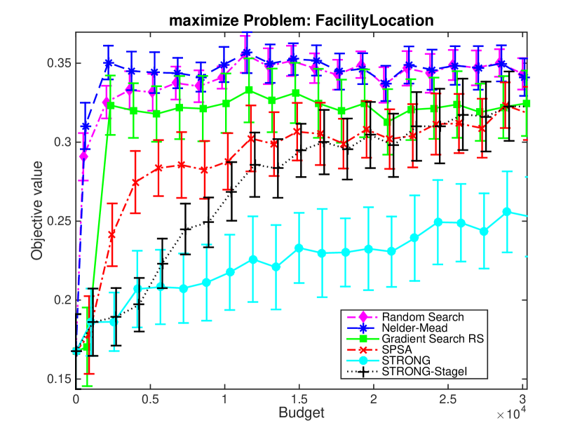
The problems Ambulance and FacilityLocation have similar problem structure, and the plots exhibit similar trends (Figure 9). Nelder-Mead is the stand-out performer, and interestingly RandomSearch performs almost as well. STRONG probably struggles due to the computational expense of iterations in Stage II.

Figure 9: (l) Ambulance: Average Performance, (r) FacilityLocation: Average Performance

Figure 10: (l) ProductionLine: Average Performance, (r) RoutePrices: Average Performance

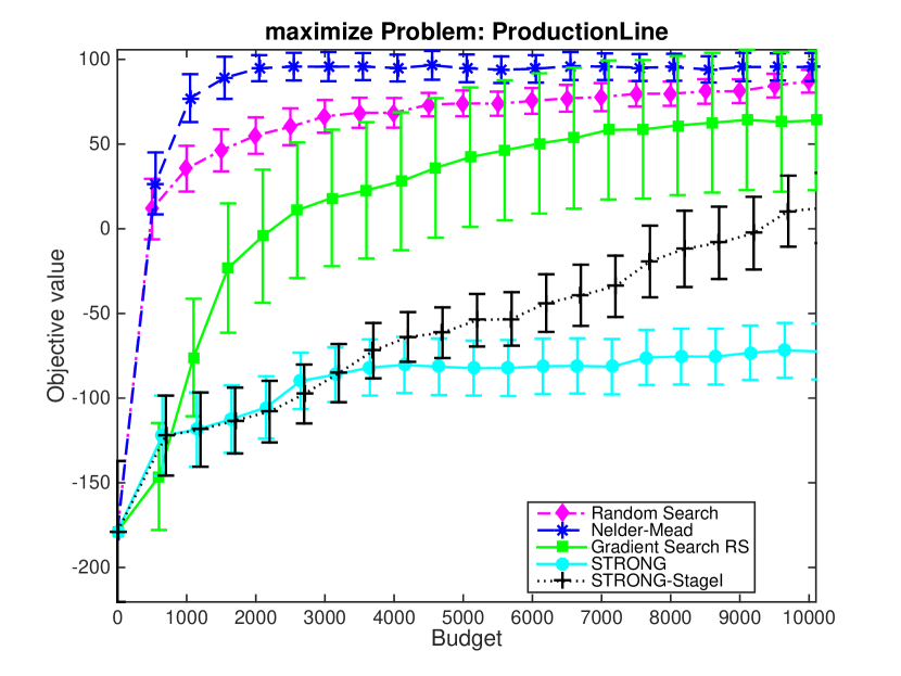
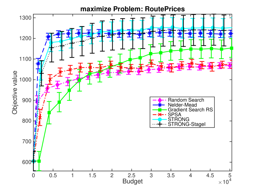
For the problem ProductionLine, all algorithms perform much as they did on the Ambulance problem, with the exception of SPSA which is excluded from Figure 10 due to numerical problems in some macro replications. The RoutePrices problem has dimension $d=12$, and accordingly RandomSearch performs poorly. Nelder-Mead, STRONG and STRONGstg1 all perform well on this problem. Of these three algorithms, Nelder-Mead is the most consistent performer across macroreplications as suggested by the narrow confidence intervals, but both trust region methods appear to identify a slightly better objective function for the maximal budget. We do not have an explanation for the poor performance of GradSearch and SPSA on this problem.

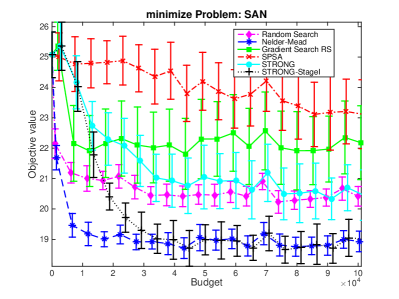
For the problem SAN (Figure 11), the strongest performers are Nelder-Mead and STRONGstg1. This problem is convex, so we would expect all algorithms to do reasonably well. Nevertheless, STRONG struggles, perhaps due to the computational effort in Stage II. GradSearch also struggles, perhaps because its test for when to perform a restart is too lenient, leading to many unproductive restarts. SPSA performs particularly poorly on this problem.

Figure 11: SAN: Average Performance

5 CONCLUSIONS

Perhaps the most important observation in our results is the robust performance of Nelder-Mead across almost all problems. It is highly deserving of further study. Interestingly, STRONGstg1 either compares similarly to, or outperforms, STRONG, calling into question the computationally expensive Stage II of STRONG. RandomSearch performed better than expected, though its performance suffers on higher-dimensional problems or on problems where the sampling distribution is poorly calibrated. SPSA performed very well on our highest-dimensional problem (in 40 dimensions), but for most problems it struggled relative to the other algorithms, including problems in dimensions 10–13. Our implementation of GradSearch performed moderately well, especially with its use of random restarts and may be worth further development.

More generally, our sense is that low-dimensional problems are over-represented in the SimOpt library. It is certainly conceivable that our observations above could change for higher-dimensional problems. The number of problems was small enough that we could present detailed results for a single problem at a time, leading to several insights. If we were to study many more problems, then this presentation would be too cumbersome and a more succinct approach would be necessary. To that end, further research on how to adapt performance profiles to simulation optimization is needed.

In this study we only tackled continuous-variable problems that are either unconstrained or box constrained (with upper and lower bounds on the variables). In future research, we would like to compare algorithms designed for discrete or integer-ordered variables, like COMPASS [6] and R-SPLINE [14].

ACKNOWLEDGMENTS

This material is based upon work supported by the National Science Foundation under grant no. CMMI-1537394, CMMI-1254298, CMMI-1536895, and IIS-1247696, by the Air Force Office of Scientific Research under grant no. FA9550-12-1-0200, FA9550-15-1-0038, and FA9550-16-1-0046, and by the Army Research Office under grant no. W911NF-17-1-0094.

References

- Amaran et al. [2016] S. Amaran, N. V. Sahinidis, B. Sharda, and S. J. Bury. Simulation optimization: a review of algorithms and applications. Annals of Operations Research, 240(1):351–380, 2016.
- Barton and Ivey Jr. [1996] R. R. Barton and J. S. Ivey Jr. Nelder-mead simplex modifications for simulation optimization. Management Science, 42(7):954–973, 1996.
- Bitbucket [2017] Bitbucket. Finitetimesimopt. https://bitbucket.org/poloczek/finitetimesimopt, 2017.
- Chang et al. [2013] K.-H. Chang, L. J. Hong, and H. Wan. Stochastic trust-region response-surface method (strong)—a new response-surface framework for simulation optimization. INFORMS Journal on Computing, 25(2):230–243, 2013.
- Dolan and Moré [2002] E. D. Dolan and J. J. Moré. Benchmarking optimization software with performance profiles. Mathematical Programming Series A, 91(2):201–213, 2002.
- Hong and Nelson [2006] J. L. Hong and B. L. Nelson. Discrete optimization via simulation using compass. Operations Research, 54(1):115–129, 2006.
- Nelder and Mead [1965] J. A. Nelder and R. Mead. A simplex method for function minimization. The computer journal, 7(4):308–313, 1965.
- Pasupathy and Henderson [2006] R. Pasupathy and S. G. Henderson. A testbed of simulation-optimization problems. In L. F. Perrone, F. P. Wieland, J. Liu, B. G. Lawson, D. M. Nicol, and R. M. Fujimoto, editors, Proceedings of the 2006 Winter Simulation Conference, pages 255–263, Piscataway, New Jersey, 2006. Institute of Electrical and Electronics Engineers, Inc.
- Pasupathy and Henderson [2011] R. Pasupathy and S. G. Henderson. Simopt: A library of simulation optimization problems. In S. Jain, R. R. Creasey, J. Himmelspach, K. P. White, and M. Fu, editors, Proceedings of the 2011 Winter Simulation Conference, pages 4075–4085, Piscataway, New Jersey, 2011. Institute of Electrical and Electronics Engineers, Inc.
- SimOpt Library [2011] SimOpt Library. Simulation optimization (simopt) library. http://www.simopt.org, 2011.
- Spall [1992] J. C. Spall. Multivariate stochastic approximation using a simultaneous perturbation gradient approximation. IEEE Transactions on Automatic Control, 37(3):332–341, 1992.
- Spall [1998] J. C. Spall. Implementation of simultaneous perturbation algorithm for stochastic optimization. IEEE Transactions on Aerospace and Electronic Systems, 34(3):817–823, 1998.
- Spall [2001] J. C. Spall. Simultaneous perturbation stochastic approximation (spsa). http://www.jhuapl.edu/SPSA/, 2001.
- Wang et al. [2013] H. Wang, R. Pasupathy, and B. W. Schmeiser. Integer-ordered simulation optimization using r-spline: Retrospective search with piecewise-linear interpolation and neighborhood enumeration. ACM Transactions on Modeling and Computer Simulation (TOMACS), 23(3):17:1–24, 2013.