Union of Intersections (UoI) for Interpretable Data Driven Discovery and Prediction

Abstract

The increasing size and complexity of scientific data could dramatically enhance discovery and prediction for basic scientific applications. Realizing this potential, however, requires novel statistical analysis methods that are both interpretable and predictive. We introduce Union of Intersections (UoI), a flexible, modular, and scalable framework for enhanced model selection and estimation. Methods based on UoI perform model selection and model estimation through intersection and union operations, respectively. We show that UoI-based methods achieve low-variance and nearly unbiased estimation of a small number of interpretable features, while maintaining high-quality prediction accuracy. We perform extensive numerical investigation to evaluate a UoI algorithm ($UoI_{Lasso}$) on synthetic and real data. In doing so, we demonstrate the extraction of interpretable functional networks from human electrophysiology recordings as well as accurate prediction of phenotypes from genotype-phenotype data with reduced features. We also show (with the $UoI_{L1Logistic}$ and $UoI_{CUR}$ variants of the basic framework) improved prediction parsimony for classification and matrix factorization on several benchmark biomedical data sets. These results suggest that methods based on the UoI framework could improve interpretation and prediction in data-driven discovery across scientific fields.

1 Introduction

A central goal of data-driven science is to identify a small number of features (i.e., predictor variables; $X$ in Fig. 1(a)) that generate a response variable of interest ($y$ in Fig. 1(a)) and then to estimate the relative contributions of these features as the parameters in the generative process relating the predictor variables to the response variable (Fig. 1(a)). A common characteristic of many modern massive data sets is that they have a large number of features (i.e., high-dimensional data), while also exhibiting a high degree of sparsity and/or redundancy [3, 41, 21]. That is, while formally high-dimensional, most of the useful information in the data features for tasks such as reconstruction, regression, and classification can be restricted or compressed into a much smaller number of important features. In regression and classification, it is common to employ sparsity-inducing regularization to attempt to achieve simultaneously two related but quite different goals: to identify the features important for prediction (i.e., model selection) and to estimate the associated model parameters (i.e., model estimation) [3, 41]. For example, the Lasso algorithm in linear regression uses $L_{1}$-regularization to penalize the total magnitude of model parameters, and this often results in feature compression by setting some parameters exactly to zero [40] (See Fig. 1(a), pure white elements in right-hand vectors, emphasized by $\times$). It is well known that this type of regularization implies a prior assumption about the distribution of the parameter (e.g., $L_{1}$-regularization implicitly assumes a Laplacian prior distribution) [25]. However, strong sparsity-inducing regularization, which is common when there are many more potential features than data samples (i.e., the so-called small $n/p$ regime) can severely hinder the interpretation of model parameters (Fig. 1(a), indicated by less saturated colors between top and bottom vectors on right hand side). For example, while sparsity may be achieved, incorrect features may be chosen and parameters estimates may be biased. In addition, it can impede model selection and estimation when the true model distribution deviates from the assumed distribution [3, 18]. This may not matter for prediction quality, but it clearly has negative consequences for interpretability, an admittedly not completely-well-defined property of algorithms that is crucial in many scientific applications [14]. In this context, interpretability reflects the degree to which an algorithm returns a small number of physically meaningful features with unbiased and low variance estimates of their contributions.

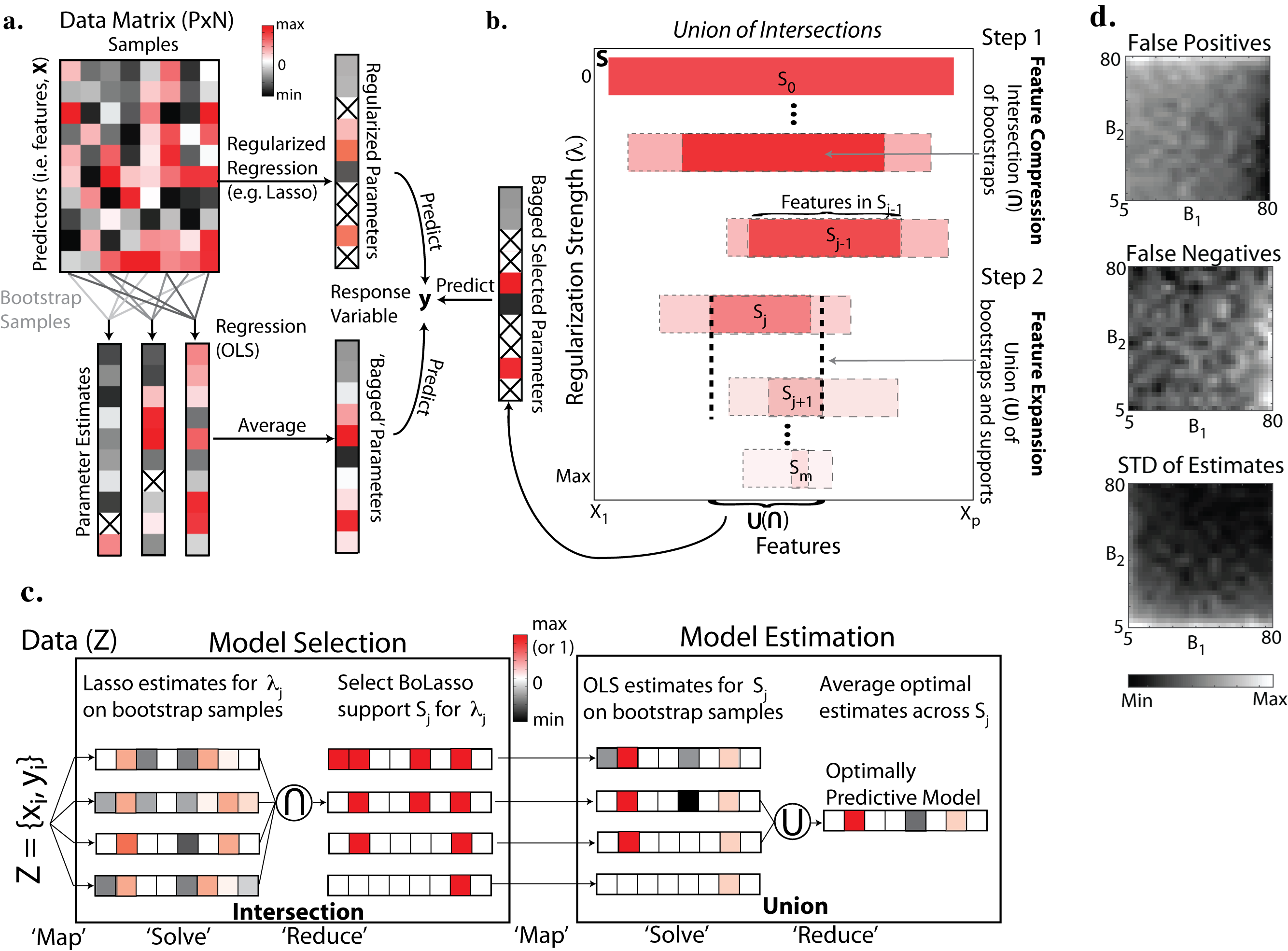
Figure 1: The basic UoI framework. (a) Schematic of regularization and ensemble methods for regression. (b) Schematic of the Union of Intersections (UoI) framework. (c) A data-distributed version of the $UoI_{Lasso}$ algorithm. (d) Dependence of false positive, false negatives, and estimation variability on number of bootstraps in selection ($B_{1}$) and estimation ($B_{2}$) modules.

On the other hand, another common characteristic of many state of the art methods is to combine several related models for a given task. In statistical data analysis, this is often formalized by so-called ensemble methods, which improve prediction accuracy by combining parameter estimates [25]. In particular, by combining several different models, ensemble methods often include more features to predict the response variables, and thus the number of data features is expanded relative to the individuals in the ensemble. For example, estimating an ensemble of model parameters by randomly resampling the data many times (e.g., bootstrapping) and then averaging the parameter estimates (e.g., bagging) can yield improved prediction accuracy by reducing estimation variability [10, 25] (See Fig. 1(a), bottom). However, by averaging estimates from a large ensemble, this process often results in many non-zero parameters, which can hinder interpretability and the identification of the true model support (compare top and bottom vectors on right hand side of Fig. 1(a)). Taken together, these observations suggest that explicit and more precise control of feature compression and expansion may result in an algorithm with improved interpretative and predictive properties.

In this paper, we introduce Union of Intersections (UoI), a flexible, modular, and scalable framework to enhance both the identification of features (model selection) as well as the estimation of the contributions of these features (model estimation). We have found that the UoI framework permits us to explore the interpretability-predictivity trade-off space, without imposing an explicit prior on the model distribution, and without formulating a non-convex problem, thereby often leading to improved interpretability and prediction. Ideally, data analysis methods in many scientific applications should be selective (only features that influence the response variable are selected), accurate (estimated parameters in the model are as close to the true value as possible), predictive (allowing prediction of the response variable), stable (e.g., the variability of the estimated parameters is small), and scalable (able to return an answer in a reasonable amount of time on very large data sets) [38, 3, 32, 18]. We show empirically that UoI-based methods can simultaneously achieve these goals, results supported by preliminary theory. We primarily demonstrate the power of UoI-based methods in the context of sparse linear regression ($UoI_{Lasso}$), as it is the canonical statistical/machine learning problem, it is theoretically tractable, and it is widely used in virtually every field of scientific inquiry. However, our framework is very general, and we demonstrate this by extending UoI to classification ($UoI_{L1Logistic}$) and matrix factorization ($UoI_{CUR}$) problems. While our main focus is on neuroscience (broadly speaking) applications, our results also highlight the power of UoI across a broad range of synthetic and real scientific data sets.

The conference version of this technical report has appeared in the Proceedings of the 2017 NIPS Conference [5].

2 Union of Intersections (UoI)

For concreteness, we consider an application of UoI in the context of the linear regression. Specifically, we consider the problem of estimating the parameters $\beta\in\mathbb{R}^{p}$ that map a $p$-dimensional vector of predictor variables $x\in\mathbb{R}^{p}$ to the observation variable $y\in\mathbb{R}$, when there are $n$ paired samples of $x$ and $y$ corrupted by i.i.d Gausian noise:

$$y=\beta^{T}x+\varepsilon,$$ (1)

where $\varepsilon\stackrel{{\scriptstyle iid}}{{\sim}}N(0,\sigma^{2})$ for each sample. When the true $\beta$ is thought to be sparse (i.e., in the $L_{0}$-norm sense), then an estimate of $\beta$ (call it $\hat{\beta}$) can be found by solving a constrained optimization problem of the form:

$$\hat{\beta}\in\mbox{argmin}_{\beta\in\mathbb{R}^{p}}\sum_{i=1}^{n}(y_{i}-\beta x_{i})^{2}+\lambda R(\beta).$$ (2)

Here, $R(\beta)$ is a regularization term that typically penalizes the overall magnitude of the parameter vector $\beta$ (e.g., $R(\beta)=\|{\beta}\|_{1}$ is the target of the Lasso algorithm).

The Basic UoI Framework. The key mathematical idea underlying UoI is to perform model selection through intersection (compressive) operations and model estimation through union (expansive) operations, in that order. This is schematized in Fig. 1(b), which plots a hypothetical range of selected features ($x_{1}:x_{p}$, abscissa) for different values of the regularization parameter ($\lambda$, ordinate), and a more detailed description of this is provided in the Appendix. In particular, UoI first performs feature compression (Fig. 1(b), Step 1) through intersection operations (intersection of supports across bootstrap samples) to construct a family ($S$) of candidate model supports (Fig. 1(b), e.g., $S_{j-1}$, opaque red region is intersection of abutting pink regions). UoI then performs feature expansion (Fig. 1(b), Step 2) through a union of (potentially) different model supports: for each bootstrap sample, the best model estimates (across different supports) is chosen, and then a new model is generated by averaging the estimates (i.e., taking the union) across bootstrap samples (Fig. 1(b), dashed vertical black line indicates the union of features from $S_{j}$ and $S_{j+1}$). Both feature compression and expansion are performed across all regularization strengths. In UoI, feature compression via intersections and feature expansion via unions are balanced to maximize prediction accuracy of the sparsely estimated model parameters for the response variable $y$.

Innovations in Union of Intersections. UoI has three central innovations: (1) calculate model supports ($S_{j}$) using an intersection operation for a range of regularization parameters (increases in $\lambda$ shrink all values $\hat{\beta}$ towards 0), efficiently constructing a family of potential model supports $\{S:S_{j}\in S_{j-k}\mbox{, for $k$ sufficiently large}\}$; (2) use a novel form of model averaging in the union step to directly optimize prediction accuracy (this can be thought of as a hybrid of bagging [10] and boosting [37]); and (3) combine pure model selection using an intersection operation with model selection/estimation using a union operation in that order (which controls both false negatives and false positives in model selection). Together, these innovations often lead to better selection, estimation and prediction accuracy. Importantly, this is done without explicitly imposing a prior on the distribution of parameter values, and without formulating a non-convex optimization problem.

The $UoI_{Lasso}$ Algorithm. Since the basic UoI framework, as described in Fig. 1(c), has two main computational modules—one for model selection, and one for model estimation—UoI is a framework into which many existing algorithms can be inserted. Here, for simplicity, we primarily demonstrate UoI in the context of linear regression in the $UoI_{Lasso}$ algorithm, although we also apply it to classification with the $UoI_{L1Logistic}$ algorithm as well as matrix factorization with the $UoI_{CUR}$ algorithm. (See the Appendix for pseudo-code for the $UoI_{Lasso}$ algorithm.) $UoI_{Lasso}$ expands on the BoLasso method for the model selection module [1], and it performs a novel model averaging in the estimation module based on averaging ordinary least squares (OLS) estimates with potentially different model supports. $UoI_{Lasso}$ (and UoI in general) has a high degree of natural algorithmic parallelism that we have exploited in a distributed Python-MPI implementation. (Fig. 1(c) schematizes a simplified distributed implementation of the algorithm, and see the Appendix for more details.) This parallelized $UoI_{Lasso}$ algorithm uses distribution of bootstrap data samples and regularization parameters (in Map) for independent computations involving convex optimizations (Lasso and OLS, in Solve), and it then combines results (in Reduce) with intersection operations (model selection module) and union operations (model estimation module). By solving independent convex optimization problems (e.g., Lasso, OLS) with distributed data resampling, our $UoI_{Lasso}$ algorithm efficiently constructs a family of model supports, and it then averages nearly unbiased model estimates, potentially with different supports, to maximize prediction accuracy while minimizing the number of features to aid interpretability.

3 Results

We start with a discussion of the basic methodological setup. The main statistical properties are discussed numerically in Section 3.2, the results of which are supported by preliminary theoretical results in the Appendix. The rest of this section describes our extensive empirical evaluation on real and synthetic data of several variants of the basic UoI framework.

3.1 Methods

All numerical results used 100 random sub-samplings with replacement of 80-10-10 cross-validation to estimate model parameters (80%), choose optimal meta-parameters (e.g., $\lambda$, 10%), and determine prediction quality (10%). Below, $\beta$ denotes the values of the true model parameters, $\hat{\beta}$ denotes the estimated values of the model parameters from some algorithm (e.g., $UoI_{Lasso}$), $S_{\beta}$ is the support of the true model (i.e., the set of non-zero parameter indices), and $S_{\hat{\beta}}$ is the support of the estimated model. We calculated several metrics of model selection, model estimation, and prediction accuracy. (1) Selection accuracy (set overlap): $1-\frac{|S_{\hat{\beta}}\Delta S_{\beta}|}{|S_{\hat{\beta}}|_{0}+|S_{\beta}|_{0}}$, where, $\Delta$ is the symmetric set difference operator. This metric ranges in $[0,1]$, taking a value of $0$ if $S_{\beta}$ and $S_{\hat{\beta}}$ have no elements in common, and taking a value of $1$ if and only if they are identical. (2) Estimation error (r.m.s): $\sqrt{\frac{1}{p}\sum{(\beta_{i}-\hat{\beta_{i}})}^{2}}$. (3) Estimation variability (parameter variance): $E[\hat{\beta}^{2}]-(E[\hat{\beta}])^{2}$. (4) Prediction accuracy ($R^{2}$): $\frac{\sum{(y_{i}-\hat{y_{i}})}^{2}}{\sum{(y_{i}-E[y])}^{2}}$. (5) Prediction parsimony (BIC): $n\log(\frac{1}{n-1}\sum_{i=1}^{n}(y_{i}-\hat{y_{i}})^{2})+\|\hat{\beta}\|_{0}\log(n)$. For the experimental data, as the true model size is unknown, the selection ratio ($\frac{\|\hat{\beta}\|_{0}}{p}$) is a measure of the overall size of the estimated model relative to the total number of parameters. For the classification task using $UoI_{L1Logistic}$, BIC was calculated as: $-2\log\ell+S_{\hat{\beta}}\log N$, where $\ell$ is the log-likelihood on the validation set. For the matrix factorization task using $UoI_{CUR}$, reconstruction accuracy was the Frobenius norm of the difference between the data matrix $A$ and the low-rank approximation matrix $A^{\prime}$ constructed from $A(:,c)$, the reduced column matrix of A: $\|A-A^{\prime}\|_{F}$, where $c$ is the set of $k$ selected columns.

3.2 Model Selection and Stability: Explicit Control of False Positives, False Negatives, and Estimate Stability

Due to the form of the basic UoI framework, we can control both false negative and false positive discoveries, as well as the stability of the estimates. For any regularized regression method like in (2), a decrease in the penalization parameter ($\lambda$) tends to increase the number of false positives, and an increase in $\lambda$ tends to increase false negatives. Preliminary analysis of the UoI framework shows that, for false positives, a large number of bootstrap resamples in the intersection step ($B_{1}$) produces an increase in the probability of getting no false positive discoveries, while an increase in the number of bootstraps in the union step ($B_{2}$) leads to a decrease in the probability of getting no false positives. Conversely, for false negatives, a large number of bootstrap resamples in the union step ($B_{2}$) produces an increase in the probability of no false negative discoveries, while an increase in the number of bootstraps in the intersection step ($B_{1}$) leads to a decrease in the probability of no false negatives. Also, a large number of bootstrap samples in union step ($B_{2}$) gives a more stable estimate. These properties were confirmed numerically for $UoI_{Lasso}$ and are displayed in Fig. 1(d), which plots the average normalized false negatives, false positives, and standard deviation of model estimates from running $UoI_{Lasso}$, with ranges of $B_{1}$ and $B_{2}$ on four different models. These results are supported by preliminary theoretical analysis of a variant of $UoI_{Lasso}$ (see Appendix). Thus, the relative values of $B_{1}$ and $B_{2}$ express the fundamental balance between the two basic operations of intersection (which compresses the feature space) and union (which expands the feature space). Model selection through intersection often excludes true parameters (i.e., false negatives), and, conversely, model estimation using unions often includes erroneous parameters (i.e., false positives). By using stochastic resampling, combined with model selection through intersections, followed by model estimation through unions, UoI permits us to mitigate the feature inclusion/exclusion inherent in either operation. Essentially, the limitations of selection by intersection are counteracted by the union of estimates, and vice versa.

3.3 $UoI_{Lasso}$ has Superior Performance on Simulated Data Sets

To explore the performance of the $UoI_{Lasso}$ algorithm, we have performed extensive numerical investigations on simulated data sets, where we can control key properties of the data. There are a large number of algorithms available for linear regression, and we picked some of the most popular algorithms (e.g., Lasso), as well as more uncommon, but more powerful algorithms (e.g., SCAD, a non-convex method). Specifically, we compared $UoI_{Lasso}$ to five other model selection/estimation methods: Ridge, Lasso, SCAD, BoATS, and debiased Lasso [25, 40, 18, 6, 4, 27]. Note that BoATS and debiased Lasso are both two-stage methods. We examined performance of these algorithms across a variety of underlying distributions of model parameters, degrees of sparsity, and noise levels. Across all algorithms examined, we found that $UoI_{Lasso}$ (Fig. 2, black) generally resulted in very high selection accuracy (Fig. 2(c), right) with parameter estimates with low error (Fig. 2(c), center-right), leading to the best prediction accuracy (Fig. 2(c), center-left) and prediction parsimony (Fig. 2(c), left). In addition, it was very robust to differences in underlying parameter distribution, degree of sparsity, and magnitude of noise. (See the Appendix for more details.)

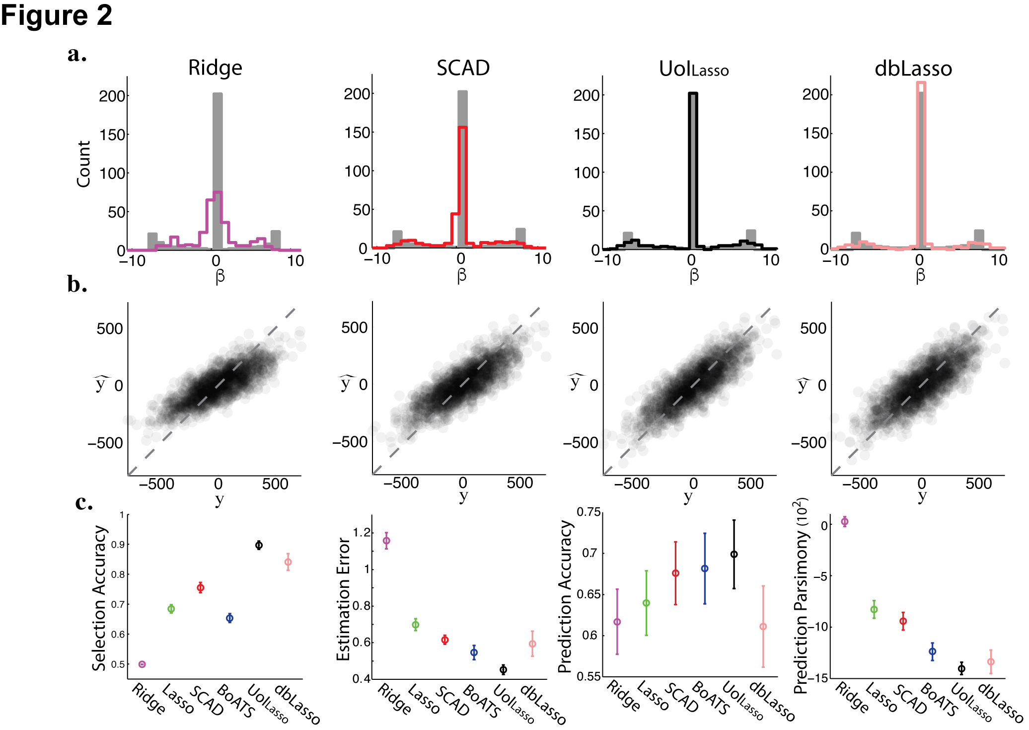
Figure 2: Range of observed results, in comparison with existing algorithms. (a) True $\beta$ distribution (grey histograms) and estimated values (colored lines). (b) Scatter plot of true and estimated values of observation variable on held-out samples. (c) Metrics of algorithm performance.

3.4 $UoI_{Lasso}$ in Neuroscience: Sparse Functional Networks from Human Neural Recordings and Parsimonious Prediction from Genetic and Phenotypic Data

We sought to determine if the enhanced selection and estimation properties of $UoI_{Lasso}$ also improved its utility as a tool for data-driven discovery in complex, diverse neuroscience data sets. Neurobiology seeks to understand the brain across multiple spatio-temporal scales, from molecules-to-minds. We first tackled the problem of graph formation from multi-electrode ($p=86$ electrodes) neural recordings taken directly from the surface of the human brain during speech production ($n=45$ trials each). See [8] for details. That is, the goal was to construct sparse neuroscientifically-meaningful graphs for further downstream analysis. To estimate functional connectivity, we calculated partial correlation graphs. The model was estimated independently for each electrode, and we compared the results of graphs estimated by $UoI_{Lasso}$ to the graphs estimated by SCAD. In Fig. 3(a)-(b), we display the networks derived from recordings during the production of /b/ while speaking /ba/. We found that the $UoI_{Lasso}$ network (Fig. 3(a)) was much sparser than the SCAD network (Fig. 3(b)). Furthermore, the network extracted by $UoI_{Lasso}$ contained electrodes in the lip (dorsal vSMC), jaw (central vSMC), and larynx (ventral vSMC) regions, accurately reflecting the articulators engaged in the production of /b/ (Fig. 3(c))  [8]. The SCAD network (Fig. 3(d)) did not have any of these properties. This highlights the improved power of $UoI_{Lasso}$ to extract sparse graphs with functionally meaningful features relative to even some non-convex methods.

We calculated connectivity graphs during the production of 9 consonant-vowel syllables. Fig. 3(e) displays a summary of prediction accuracy for $UoI_{Lasso}$ networks (red) and SCAD networks (black) as a function of time. The average relative prediction accuracy (compared to baseline times) for the $UoI_{Lasso}$ network was generally greater during the time of peak phoneme encoding [T $=$ -100:200] compared to the SCAD network. Fig. 3(f) plots the time course of the parameter selection ratio for the $UoI_{Lasso}$ network (red) and SCAD network (black). The $UoI_{Lasso}$ network was consistently $\sim 5\times$ sparser than the SCAD network. These results demonstrate that $UoI_{Lasso}$ extracts sparser graphs from noisy neural signals with a modest increase in prediction accuracy compared to SCAD.

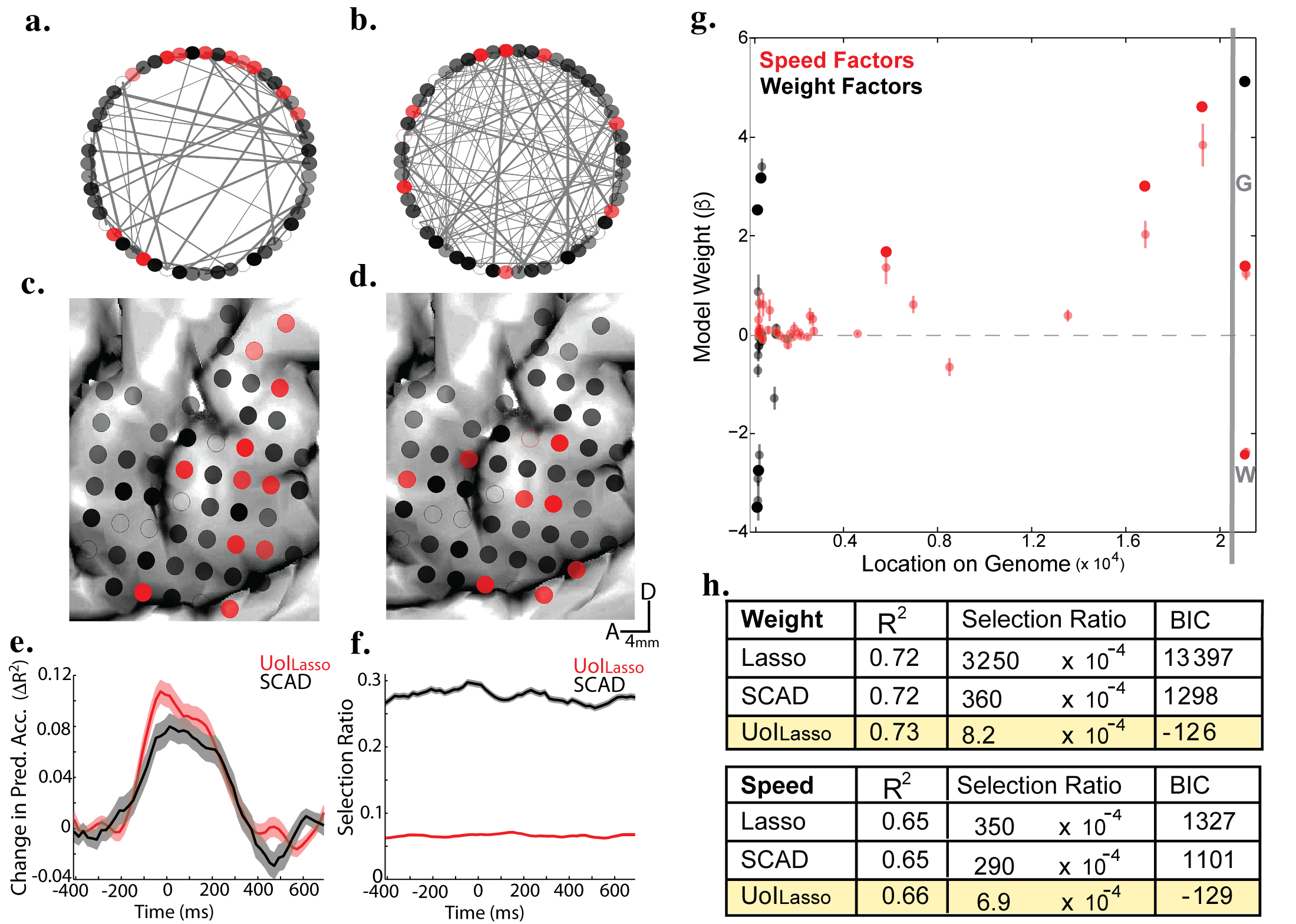
Figure 3: Application of UoI to neuroscience and genetics data. (a)-(f): Functional connectivity networks from ECoG recordings during speech production. (g)-(h): Parsimonious prediction of complex phenotypes form genotype and phenotype data.

We next investigated whether $UoI_{Lasso}$ would improve the identification of a small number of highly predictive features from genotype-phenotype data. To do so, we analyzed data from $n=365$ mice ($173$ female, $192$ male) that are part of the genetically diverse Collaborative Cross cohort. We analyzed single-nucleotide polymorphisms (SNPs) from across the entire genome of each mouse ($p=11,563$ SNPs). For each animal, we measured two continuous, quantitative phenotypes: weight and behavioral performance on the rotorod task (see [31] for details). We focused on predicting these phenotypes from a small number of geneotype-phenotype features. We found that $UoI_{Lasso}$ identified and estimated a small number of features that were sufficient to explain large amounts of variability in these complex behavioral and physiological phenotypes. Fig. 3(g) displays the non-zero values estimated for the different features (e.g., location of loci on the genome) contributing to the weight (black) and speed (red) phenotype. Here, non-opaque points correspond to the mean $\pm$ s.d. across cross-validation samples, while the opaque points are the medians. Importantly, for both speed and weight phenotypes, we confirmed that several identified predictor features had been reported in the literature, though by different studies, e.g., genes coding for Kif1b, Rrm2b/Ubr5, and Dloc2. (See the Appendix for more details.) Accurate prediction of phenotypic variability with a small number of factors was a unique property of models found by $UoI_{Lasso}$. For both weight and rotorod performance, models fit by $UoI_{Lasso}$ had marginally increased prediction accuracy compared to other methods ($+1\%$), but they did so with far fewer parameters (lower selection ratios). This results in prediction parsimony (BIC) that was several orders of magnitude better (Fig. 3(h)). Together, these results demonstrate that $UoI_{Lasso}$ can identify a small number of genetic/physiological factors that are highly predictive of complex physiological and behavioral phenotypes.

3.5 $UoI_{L1Logistic}$ and $UoI_{CUR}$: Application of UoI to Classification and Matrix Decomposition

As noted, UoI is is a framework into which other methods can be inserted. While we have primarily demonstrated UoI in the context of linear regression, it is much more general than that. To illustrate this, we implemented a classification algorithm ($UoI_{L1Logistic}$) and matrix decomposition algorithm ($UoI_{CUR}$), and we compared them to the base methods on several data sets (see Appendix for details). In classification, UoI resulted in either equal or improved prediction accuracy with 2x-10x fewer parameters for a variety of biomedical classification tasks (Fig. 4(a)). For matrix decomposition (in this case, column subset selection), for a given dimensionality, UoI resulted in reconstruction errors that were consistently lower than the base method (BasicCUR), and quickly approached an unscalable greedy algorithm (GreedyCUR) for two genetics data sets (Fig. 4(b)). In both cases, UoI improved the prediction parsimony relative to the base (classification or decomposition) method.

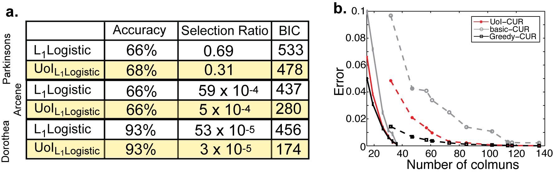
Figure 4: Extension of UoI to classification and matrix decomposition. (a) UoI for classification ($UoI_{L1Logistic}$). (b) UoI for matrix decomposition ($UoI_{CUR}$); solid and dashed lines are for PAH and dashed SORCH data sets, respectively.

4 Discussion

UoI-based methods leverage stochastic data resampling and a range of sparsity-inducing regularization parameters/dimensions to build families of potential features, and they then average nearly unbiased parameter estimates of selected features to maximize predictive accuracy. Thus, UoI separates model selection with intersection operations from model estimation with union operations: the limitations of selection by intersection are counteracted by the union of estimates, and vice versa. Stochastic data resampling can be a viewed as a perturbation of the data, and UoI efficiently identifies and robustly estimates features that are stable to these perturbations. A unique property of UoI-based methods is the ability to control both false positives and false negatives. Initial theoretical work (see Appendix) shows that increasing the number of bootstraps in the selection module ($B_{1}$) increases the amount of feature compression (primary controller of false positives), while increasing the number of bootstraps in the estimation module ($B_{2}$) increases feature expansion (primary controller of false negatives), and we observe this empirically. Thus, neither should be too large, and their relative values express the balance between feature compression and expansion. This tension is seen in many places in machine learning and data analysis: local nearest neighbor methods vs. global latent factor models; local spectral methods that tend to expand due to their diffusion-based properties vs. flow-based methods that tend to contract; and sparse $L_{1}$ vs. dense $L_{2}$ penalties/priors more generally. Interestingly, an analogous balance of compressive and expansive forces contributes to neural leaning algorithms based on Hebbian synaptic plasticity [7]. Our results highlight how revisiting popular methods in light of new data science demands can lead to still further-improved methods, and they suggest several directions for theoretical and empirical work.

Appendix A Additional Material

In this appendix section, we will provide additional information about the UoI method. We will start in Section A.1 with an extended introduction for scientific data. Then, in Section A.2, we provide pseudo-code for $UoI_{Lasso}$; in Section A.3, we discuss scaling issues; in Section A.4, we describe preliminary theoretical analysis of Union of Intersections; in Section LABEL:sxn:app-more_simulated, we discuss expanded results for the simulated data example; in Section LABEL:sxn:app-dstbns_sparsity, we discuss simulated data across different parameter distributions and levels of sparsity; in Section LABEL:sxn:app-noise, we discuss simulated data across different noise magnitudes; in Section LABEL:sxn:app-logistic, we discuss $UoI_{L1Logistic}$ for classification problems; and in Section LABEL:sxn:app-uoi_cur, we discuss $UoI_{CUR}$ for applying matrix decompositions to genetics data. We conclude in Section LABEL:sxn:app-discussion with a brief additional discussion and conclusion.

A.1 Extended Introduction for Scientific Examples

An important aspect of the use of machine learning and data analysis techniques in scientific applications—as opposed to internet, social media, and related applications—is that scientific researchers often implicitly or explicitly interpret the output of their data analysis tools as reflecting the true state of nature. For example, in neuroscience, one often wants to understand how neural activity (e.g., action potentials, calcium transients, cortical field potentials, etc.) is mapped to features of the external world (e.g., sounds or movement), or to features of the brain itself (e.g., the activity of other brain areas) [15]. A common approach to this is to formulate the mapping as a parametric model and then estimate the model parameters from noisy data. In addition to providing predictive capabilities, such model parameters can also provide insight into neural representations, functional connectivity, and population dynamics [36, 39, 6]. Indeed, this insight into the underlying neuroscience is typically at least as important as the predictive quality of the model. Likewise, in molecular biology and medicine, recent advances have allowed for the proliferation of low-cost whole-genome mapping, paving the way for large-scale genome wide association studies (GWAS) [42]. The relationship between genetic variations and observed phenotypes can be estimated from a parametric model [19, 12, 43]. Here, researchers may be interested in methods that allow for the identification of low-penetrance genes that are present at high frequency in a population, as these are likely the major genetic components associated with predisposition to disease risk and other physiological and behavioral phenotypes [28, 24]. Because the molecules encoded by the genes are often used to guide future experiments or drug development, identifying a small number of genetic factors that are highly predictive is critical to accelerate basic discovery and targets for next generation therapeutics. These and other examples [14] illustrate that the prediction-versus-interpretation data analysis needs of the scientific community are not well aligned with the needs of the Internet and social media industries that are forcing functions for the development of many machine learning and data analysis methods.

A.2 Pseudo-code for the $UoI_{Lasso}$ Algorithm

Here, we provide pseudo-code for a $UoI_{Lasso}$ algorithm.

Algorithm: $UoI_{Lasso}$

Input: data (X,Y) $\in\mathbb{R}^{n\times(p+1)}$;
vector of regularization parameters $\lambda\in\mathbb{R}^{q}$;
number of bootstraps $B_{1}$ and $B_{2}$;

% Model Selection
for k=1 to $B_{1}$ do
Generate bootstrap sample $T^{k}=(X^{k}_{T},Y^{k}_{T})$
for $\lambda_{j}\in\lambda$ do
Compute Lasso estimate ${}^{j}\hat{\beta}^{k}$ from $T^{k}$
Compute support $S^{k}_{j}=\{i\}$ s.t. ${}^{j}\hat{\beta}^{k}_{i}\neq 0$
end for
end for
for j=1 to q do
Compute BoLasso support for $\lambda_{j}:S_{j}=\smashoperator[]{\bigcap_{}^{}}^{B_{1}}_{k=1}S^{k}_{j}$
end for

% Model Estimation
for k=1 to $B_{2}$ do
Generate bootstrap samples for cross-validation:
training $T^{k}=(X^{k}_{T},Y^{k}_{T})$
evaluation $E^{k}=(X^{k}_{E},Y^{k}_{E})$
for j=1 to q do
Compute OLS estimate $\hat{\beta}^{k}_{S_{j}}$ from $T^{k}$
Compute loss on $E^{k}:L(\hat{\beta}^{k}_{S_{j}},E^{k})$
end for
Compute best model for each bootstrap sample:
$\hat{\beta}^{k}_{S}=\operatornamewithlimits{argmin}\limits_{\hat{\beta}^{k}_{S_{j}}}L(\hat{\beta}^{k}_{S_{j}},E^{k})$
end for
Compute bagged model estimate $\hat{\beta}^{*}=\frac{1}{B_{2}}\smashoperator[r]{\sum_{k=1}^{B_{2}}}\hat{\beta}^{k}_{S}$
Return: $\hat{\beta}^{*}$

As described in the main text, UoI is a framework that includes performing complementary unions and intersections of a basic underlying method. When applied to $L_{1}$-regularized $L_{2}$ regression, we obtain the $UoI_{Lasso}$ algorithm. This pseudo-code implements a serial version of the $UoI_{Lasso}$ algorithm. The algorithm uses the BoLasso method for the model selection through the intersection module, and bagged ordinary least squares regression for the the estimation through the union module. This algorithm is described serially, but, as schematized in Fig. 1(c), this algorithm has a great deal of natural parallelism, involving independent calculations across different bootstrap samples ($B_{1}$ and $B_{2}$) and values of the regularization parameter ($\lambda$), which occur for both the selection and estimation modules. Of course, further algorithmic parallelization can be achieved by distributing the computations required for solving the Lasso and OLS convex-optimization steps, using, e.g., the Alternating Directions Method of Multiplies (ADMM). Even for linear regression, other methods could be used for the selection module (e.g., SCAD, stability selection, etc.), though keeping the estimation module as an un-regularized method should be maintained. When other base algorithms are used, e.g., a logistic classifier or a CUR matrix decomposition, then other variants of the basic UoI framework, such as $UoI_{L1Logistic}$ and $UoI_{CUR}$ (that are described below and in the main text), are obtained.

A.3 Scaling of the $UoI_{Lasso}$ Algorithm

$UoI_{Lasso}$ (and UoI in general) has a high degree of natural algorithmic parallelism that we have exploited in a distributed Python-MPI implementation. (See Section 3.1 also.) To assess the scalability of the algorithm, we carried out a series of scaling computations with data sets of different sizes; and, in Fig. 5, we present a summary of the performance between a serial and a distributed implementation of $UoI_{Lasso}$. We used the computational runtime and the input-output (IO) time as performance indicators. We used artificially generated data sets with sizes that ranged from 400 bytes to 40 gigabytes, therefore spanning 5 orders of magnitude in size, and we performed computations on a supercomputer (NERSC at LBNL), as described in Section 3.1. Fig. 5(a) shows the computational runtime for the distributed and the serial program compared across data set sizes, as indicated by the gray scale color and the legend. All data points in Fig 5(a) lie well above the identity line shown as a diagonal gray dashed line, which indicates that runtime was in all cases notably lower for the distributed version of $UoI_{Lasso}$. This improvement in runtime increased with the data set size: the best-fit line to the (log-log) data had a slope of 1.19 and y-intercept of 2.13. This indicates a general improvement of approximately two-orders of magnitude (y-intercept), and that improvements get better for larger data sets (slope greater than 1). The computational runtime is also shown in Fig. 5(b) with pink and gray bars, and in addition this plot includes the IO time shown with red and black bars for the parallel and serial versions of $UoI_{Lasso}$, respectively. We found that even though IO time was slightly larger in the parallel version for small data sets, IO operations benefited from the distributed implementation when large datasets were analyzed. Overall, these results show a good scalability, in parallel settings, of the basic UoI framework, illustrating its potential applicability to very large-scale data sets.

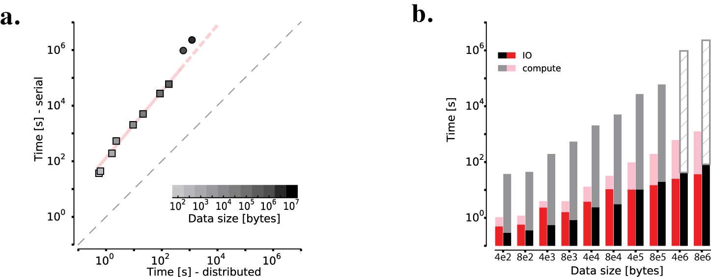
Figure 5: Efficient and scalable implementation of $UoI_{Lasso}$ on distributed computing systems. (a) Comparison of computational runtime between serial and distributed $UoI_{Lasso}$, as a function of the data set size. Gray-scale: size of the design matrix in bytes (legend). Circular markers: computational runtime of serial $UoI_{Lasso}$ was estimated using a single iteration. Square markers: actual data points. Red line: linear fit to the actual (log-log) data (squares). Grey dashed line is unity. (b) Computational runtime and data IO time for serial (grey/black) and distributed (pink/red) $UoI_{Lasso}$ as a function of data set size (x-axis). Hatched bars: estimated runtime time using a single iteration.

A.4 Theory

In section  3.2, we make certain statements regarding the control of false negative and false positive discoveries in $UoI_{Lasso}$ method and the relationship of the control of false positive and false negative discoveries in $UoI_{Lasso}$ method with the bootstrap parameters $B_{1}$ and $B_{2}$. The bootstrap parameter $B_{1}$ is used in the model selection or intersection step of the $UoI_{Lasso}$ algorithm. The model selection step derives from the BoLasso algorithm [1]. As shown in Lemma LABEL:lemma:bach in section LABEL:sxn:bolasso, for correct model selection with high probability, we should have $B_{1}\rightarrow\infty$ but at a rate slower than $\log n$ for BoLasso. But for theoretical analysis of the model estimation step of $UoI_{Lasso}$ algorithm, we need separate control on the false positives (regression coefficients falsely estimated as non-zero) and false negatives (regression coefficients falsely estimated as zero) of the recovered support. In Lemma LABEL:lemma:bach, the result gives a bound on total error in support recovery, but not separate control on false positives and false negatives. For this reason, in the theoretical analysis of UoI methods, in stead of using BoLasso in the model selection step, we use stability selection [33], as there are some better theoretical properties available for the stability selection method. We give the pesudo-code of the modified algorithm, $\text{UoI}^{\text{stable}}_{\text{Lasso}}$, in section A.4.1. Since, the bootstrap parameter for model selection step of $UoI_{Lasso}$, $B_{1}$, is not a parameter of the algorithm $\text{UoI}^{\text{stable}}_{\text{Lasso}}$, the main theoretical results proved for $\text{UoI}^{\text{stable}}_{\text{Lasso}}$ establish relationships between the false positive and false negative control and $B_{2}$, the bootstrap parameter for the model estimation step.

Let us consider that we have data $(Y_{1},\boldsymbol{X}_{1}),\ldots,(Y_{n},\boldsymbol{X}_{n})$ with univariate response variable $Y_{i}$ and $p$-dimensional predictor variable $\boldsymbol{X}_{i}$ for each sample, $i\in\{1,\ldots,n\}$. The vectors $(Y_{i},\boldsymbol{X}_{i})$ are assumed independent with common distribution in $\mathbb{R}^{p+1}$ for each $i\in\{1,\ldots,n\}$. Consider the linear regression model for the data

$$\boldsymbol{Y}=\boldsymbol{X}\boldsymbol{\beta}+\boldsymbol{\varepsilon}$$ (3)

where, $\boldsymbol{Y}=(Y_{1},\ldots,Y_{n})$, $\boldsymbol{X}$ is the $n\times p$ random design matrix of explanatory variables and $\boldsymbol{\varepsilon}=(\varepsilon_{1},\ldots,\varepsilon_{n})$ are random noise terms with $\boldsymbol{\varepsilon}\stackrel{{\scriptstyle iid}}{{\sim}}N(0,\sigma^{2}\mathbf{I}_{n})$ and $\boldsymbol{X}_{i}$ are orthogonal to $\varepsilon_{i}$ for each $i\in\{1,\ldots,n\}$, that is, $\mathbb{E}(X_{ij}\varepsilon_{i})=0$ for $j=1,\ldots,p$. Also, the design matrix has the property $\sum_{i=1}^{n}\boldsymbol{X}_{ij}^{2}=1$ for all $j=1,\ldots,p$. Let $S$ be the set of non-zero coefficients of $\boldsymbol{\beta}$ with $|S|=s$; $N$ be the set of zero coefficients of $\boldsymbol{\beta}$ with $|N|=p-s$. We consider that $s$ is constant and $p$ can be function of $n$, the sample size.

Consider the lasso regression problem with regularization parameter $\lambda>0$, as minimizing the following optimization function with respect to $\boldsymbol{\beta}$,

$$L(\boldsymbol{\beta},\lambda)=\left|\left|\boldsymbol{Y}-\boldsymbol{X}\boldsymbol{\beta}\right|\right|_{2}^{2}+\lambda||\boldsymbol{\beta}||_{1}$$ (4)

A.4.1 $UoI_{Lasso}$ Algorithm with Stability Selection

Here we present a preliminary theoretical analysis of Union of Intersections for Lasso based regression. The $UoI_{Lasso}$ algorithm is presented in section A.2. The algorithm analyzed in this section differs slightly from the $UoI_{Lasso}$ algorithm in that it uses the stability selection method of Meinshausen and Buhlmann (2010) [33] instead of BoLasso in the model selection step. This was for tractability, as the current analytical results for stability selection are more amenable to theoretical analysis in the UoI framework. A brief review of the results on BoLasso is given in section LABEL:sxn:bolasso. As noted in [33], there is a great deal of similarity between stability selection and BoLasso. The stability selection method proposed in [33] has two hyperparameters, $\alpha\in\mathbb{R}_{+}$ (where, $\mathbb{R}_{+}=\{x\in\mathbb{R}|x>0\}$) and $\pi_{thr}\in[0,1]$ (for details, see [33]). As mentioned in [33], the stability selection algorithm is similar to the BoLasso algorithm for $\pi_{thr}=1$.

Here, we provide pseudo-code for $\text{UoI}^{\text{stable}}_{\text{Lasso}}$ algorithm.

Algorithm: $\text{UoI}^{\text{stable}}_{\text{Lasso}}$

Input: data (X,Y) $\in\mathbb{R}^{n\times(p+1)}$;
vector of regularization parameters $\boldsymbol{\lambda}\in\mathbb{R}_{+}^{q}$;
Stability selection hyperparameters $\alpha\in\mathbb{R}_{+}$ and $\pi_{thr}\in(0,1)$;
number of bootstraps $B_{2}$;

% Model Selection
for j=1 to q do
Compute stability selection support for $\lambda_{j}:S_{j}$, by running the stability selection algorithm from [33] with hyperparameters $(\alpha,\pi_{thr},\lambda_{j})$ on data $(\boldsymbol{Y},\boldsymbol{X})$.
end for

% Model Estimation
for k=1 to $B_{2}$ do
Generate bootstrap samples for cross-validation:
training $T^{k}=((X^{k}_{T})_{n_{1}\times p},(Y^{k}_{T})_{n_{1}\times 1})$
evaluation $E^{k}=((X^{k}_{E})_{n_{2}\times p},(Y^{k}_{E})_{n_{2}\times 1})$
for j=1 to q do
Compute OLS estimate $\hat{\beta}^{k}_{S_{j}}$ from $T^{k}$
Compute loss on $E^{k}:L(\hat{\beta}^{k}_{S_{j}},\lambda_{j})$
end for
Compute best model for each bootstrap sample:
$\hat{\beta}^{k}_{S}=\operatornamewithlimits{argmin}\limits_{\hat{\beta}^{k}_{S_{j}}:j=1,\ldots p}L(\hat{\beta}^{k}_{S_{j}},\lambda_{j})$
end for
Compute bagged model estimate $\hat{\beta}^{stable}_{UoI}=\frac{1}{B_{2}}\smashoperator[r]{\sum_{k=1}^{B_{2}}}\hat{\beta}^{k}_{S}$
Return: $\hat{\beta}^{stable}_{UoI}$

Based on the estimate $\hat{\beta}^{stable}_{UoI}$, we define the support of the coefficient estimate as the set of non-zero coefficients of $\hat{\beta}^{stable}_{UoI}$. We call the support set to be $\hat{S}^{UoI}_{B_{2}}\equiv\{j\in\{1,\ldots,p\}|(\beta^{stable}_{UoI})_{j}\neq 0\}$. The $\text{UoI}^{\text{stable}}_{\text{Lasso}}$ algorithm works in two parts. In the first part, that is the model selection step, a support set for the coefficients is obtained for each $\lambda\in\boldsymbol{\lambda}$ (where, $\boldsymbol{\lambda}$ is the set of regularization parameters) based on stability selection algorithm. In the second part, that is the model estimation step, a least squares estimate is obtained using the support set obtained from model selection step for $B_{2}$ bootstrap samples of the data and for each $\lambda\in\boldsymbol{\lambda}$. For each bootstrap sample, the best coefficient estimate corresponding to the regularization parameter $\lambda$ with minimum prediction error is recorded. A new estimate of the regression coefficients is obtained by taking the average of the best estimates obtained for each bootstrap sample. Thus the support of the regression coefficient estimate ultimately obtained is found after the union of the support of several stability selection based estimates.

Another set of notations is needed for theoretical analysis of the $\text{UoI}^{\text{stable}}_{\text{Lasso}}$ algorithm. For any $A\subseteq\{1,\ldots,p\}$, define the sub-design and sub-Gram matrices as

$$X_{A}\equiv(X^{j},j\in A)_{n\times|A|},\ \ \ \Sigma_{A}=X_{A}^{T}X_{A}$$ (5)

where, $X^{j}$ is the $j$-th column of design matrix or the observations corresponding to $j$-th predictor variable.

We consider several assumptions on the set-up to prove the theoretical results for the $\text{UoI}^{\text{stable}}_{\text{Lasso}}$ algorithm. The assumptions (A1)-(A2) are required for properly defining the linear model. The assumption (A1) states the condition on the random design matrix set up. It states the assumption of independence of data and independence between explanatory variables and error variables. It also gives condition on the distribution of the response and explanatory variables. The assumption (A2) specifies the linear model and homoscedasticity assumptions. Assumption (A3) gives condition on the covariance matrix of the design or explanatory variables. The bound on the ratio of largest and smallest eigenvalues of sub-matrices of covariance matrix of explanatory variables given in (A3) is required in proving the results on model selection as well as model estimation step. Lastly, the assumption (A4) states the restriction on the size of the bootstrap training and validation samples in the model estimation step. The condition (A4) is needed so that both estimation of parameters using training sample and estimation of regularization parameters using validation sample have nice large sample properties.

Assumption:

• The vectors $(\boldsymbol{Y}_{i},\boldsymbol{X}_{i})$ are assumed independent with common (unknown) distribution in $\mathbb{R}^{p+1}$. The cumulant generating functions $\mathbb{E}(\exp(z||X||_{2}^{2}))$ and $\mathbb{E}(\exp(zY^{2}))$ are finite for some $z>0$. Also, $Y_{i}-X_{i}\boldsymbol{\beta}$ is orthogonal to $X_{i}$, that is, $\mathbb{E}(X_{ij}\boldsymbol{\varepsilon}_{i})=0$ for $i=1,\ldots,n$ and $j=1,\ldots,p$, where, $\boldsymbol{\varepsilon}_{i}=Y_{i}-X_{i}\boldsymbol{\beta}$.

• $\mathbb{E}(\boldsymbol{Y}|\boldsymbol{X})=\boldsymbol{X}^{T}\boldsymbol{w}$ and $\mbox{Var}(\boldsymbol{Y}|\boldsymbol{X})=\sigma^{2}$ a.s. for some $\boldsymbol{w}\in\mathbb{R}^{p}$ and $\sigma\in\mathbb{R}_{+}$.

• We consider the sparse Reisz condition (SRC) as given in [33]. Let us consider that there exists functions $c_{min}:\{1,\ldots,p\}\rightarrow\mathbb{R}_{+}$ and $c_{max}:\{1,\ldots,p\}\rightarrow\mathbb{R}_{+}$, such that for $d\in\mathbb{Z}$, $d>0$, we have,

  $$c_{min}(d)\leq\min_{|A|\leq d}\phi_{min}(\Sigma_{A})\leq\max_{|A|\leq d}\phi_{max}(\Sigma_{A})\leq c_{max}(d)$$ (6)

  where, $\phi_{min}(M)$ and $\phi_{max}(M)$ are the minimum and maximum eigenvalues of a matrix $M$. In that case, we assume that there exists some constant $C>1$ and some constant $\kappa\geq 9$, such that,

  $$\frac{c_{max}(Cs^{2})}{c_{\min}^{3/2}(Cs^{2})} < \sqrt{C}\kappa$$

  with probability, $p_{s}$, where, $p_{s}\rightarrow 1$, as $n,p\rightarrow\infty$.

• The number of training and validation samples in the model selection step, $n_{1}$ and $n_{2}$ should follow the relation that $n_{1}=c_{1}n$ and $n_{2}=c_{2}n$, where, $0<c_{1},c_{2}<1$ are constants (not dependent on $p$).

Under the assumptions (A1)-(A4) on the linear model setup, we prove the following result on model selection and model estimation accuracy of the UoI procedure. Note that, we denote, $(a\wedge b):=\min\{a,b\}$.

Theorem 1.

Consider the model in (3) and the assumptions (A1)-(A4) is satisfied.

• Model selection step: Consider $\alpha$ given by $\alpha^{2}=\nu c_{min}(m)/m$, for any $\nu\in((7/\kappa)^{2},1/\sqrt{2})$, and $m=Cs^{2}$, for some constant $C>1$. Let $a_{n}$ be a sequence with $a_{n}\rightarrow\infty$ for $n\rightarrow\infty$. Let $\lambda_{min}=2\sigma(\sqrt{2C}s+1)\sqrt{\log(p\wedge a_{n})/n}$ and assume that $p>10$ and $s\geq 7$. Then, there exists some $\delta=\delta_{s}\in(0,1)$ such that for all $\pi_{thr}\geq 1-\delta$, there exists a set $\Omega_{1}$ with $\mathrm{P}(\Omega_{1})\geq p_{s}(1-5/(p\wedge a_{n}))$, such that for data set $(Y_{i},\boldsymbol{X}_{i})_{i=1}^{n}$ arising from such a set,

  $$N\cap\hat{S}_{\lambda}^{stable}=\emptyset,$$ (7)

  where $\hat{S}^{stable}_{\lambda}=$ support selected by stability selection with $\lambda\geq\lambda_{min}$. On the same set $\Omega_{1}$,

  $$(S\backslash S_{small;\lambda})\subseteq\hat{S}^{stable}_{\lambda}$$ (8)

  where $S_{small;\lambda}=\{k:|\beta_{k}|\leq 0.3(Cs)^{3/2}\lambda\}$.

• Model estimation step: For a set $\Omega$ such that $\mathrm{P}(\Omega)\geq\min\left\{1-(1-p_{W})^{B_{2}},(p_{W})^{B_{2}}\right\}$, where, $p_{W}=p^{2}_{s}(1-5/(p\wedge a_{n}))$ and for data $(\boldsymbol{Y}_{i},\boldsymbol{X}_{i})_{i=1}^{n}$ as element of the set $\Omega$, we have,

  $$N\cap\hat{S}^{UoI}_{B_{2}}=\emptyset$$ (9)

  where $\hat{S}^{UoI}_{B_{2}}=$ support selected after model estimation step. On the same set $\Omega$,

  $$(S\backslash S_{small;\lambda_{min}})\subseteq\hat{S}^{UoI}_{B_{2}}$$ (10)

  where, $S_{small;\lambda_{min}}=\{k:|\beta_{k}|\leq 0.3(Cs)^{3/2}\lambda_{min}\}$.

• Estimation Accuracy: On the same set $\Omega$ as in (b), for data $(\boldsymbol{Y}_{i},\boldsymbol{X}_{i})_{i=1}^{n}$ as element of the set $\Omega$, we have,

  $$\left|\left|X(\hat{\beta}^{stable}_{UoI}-\beta)\right|\right|^{2}\leq C_{1}\sigma^{2}\frac{\log p}{n}$$ (11)

  for some constant $C_{1}>0$.

Comments: The following observations can be made from the above Theorem 1.

• Explanation. In part (a) and (b) of the Theorem, equations (7) and (9), the results imply that no noise variables are selected. In equation (8) and (10), the results imply that all variables with sufficiently large regression coefficient are selected.

• Control of false positive discoveries. The control of false positive discoveries is achieved both in the model selection and model estimation steps. The probability of having no false positives in the model selection step, $p_{s}\left(1-\frac{5}{p\wedge a_{n}}\right)$, which tends to one as $p,n\rightarrow\infty$. Although it is not explicitly stated in the Theorem, it becomes apparent from the proof that the union step that the probability of having no false positives to $p_{W}^{B_{2}}$, where, $p_{W}=p^{2}_{s}\left(1-5/(p\wedge a_{n})\right)$, which tend to one as $n,p\rightarrow\infty$. Note that, the probability of having no false positives decreases in the model estimation step to $p_{W}^{B_{2}}$ from $p_{s}\left(1-\frac{5}{p\wedge a_{n}}\right)$ in model selection step for $B_{2}\geq 1$. Also, $p_{W}^{B_{2}}\rightarrow 1$ if $B_{2}\rightarrow\infty$ slow enough.

• Control of false negative discoveries. The control of false negative discoveries is also achieved both in the model selection and model estimation steps. The maximum size of false negatives in the model selection step is $S_{small;\lambda}=\{k:|\beta_{k}|\leq 0.3(Cs)^{3/2}\lambda\}$ for each $\lambda\in\boldsymbol{\lambda}$ and such false negatives occur with probability $p_{s}\left(1-\frac{5}{p\wedge a_{n}}\right)$, which tends to one as $p,n\rightarrow\infty$. Although it is not explicitly stated in the Theorem, the model estimation step both decreases the probability of having false negatives as well as reduces the size of the false negatives. The maximum size of false negatives in the model estimation step is $S_{small;\lambda_{min}}=\{k:|\beta_{k}|\leq 0.3(Cs)^{3/2}\lambda_{min}\}$ and such false negatives occur with probability $(1-(1-p_{W})^{B_{2}})$. So, the maximum size of false negatives after the model estimation step, $S_{small;\lambda_{min}}$, becomes smaller than the size $S_{small;\lambda}$ obtained after model selection step for $\lambda\geq\lambda_{min}$. The number of non-zero parameter values estimated as zero becomes small with probability $(1-(1-p_{W})^{B_{2}})$, where, $p_{W}=p^{2}_{s}(1-5/(p\wedge a_{n}))$, which tends to one as $n,p\rightarrow\infty$. Thus, a large number of bootstrap resamples in the model estimation step ($B_{2}$) produce an increase in the probability of having small false negative discoveries. Also, the probability increases in the model estimation step to $(1-(1-p_{W})^{B_{2}})$ from $p_{s}\left(1-\frac{5}{p\wedge a_{n}}\right)$ in model selection step for large enough $B_{2}$. Thus the $\text{UoI}^{\text{stable}}_{\text{Lasso}}$ algorithm improves upon the stability selection results.

• Model selection in the whole UoI operation. After the model estimation step, we have correct model selection with high probability for the entire UoI procedure if both the probabilities $(1-(1-p_{W})^{B_{2}})$ and $p_{W}^{B_{2}}$ are large.

• Estimation Accuracy. The estimation accuracy of the $\text{UoI}^{\text{stable}}_{\text{Lasso}}$ estimators occurs at the same rate as Lasso but with probability as $\min\left\{1-(1-p_{W})^{B_{2}},(p_{W})^{B_{2}}\right\}$.

A.4.2 Proof of Theorem 1

For the sake of clarity, we redefine several notations. Let us consider the estimated coefficient parameter and the set of selected variables from stability selection (or model selection step) for any regularization parameter $\lambda\in\mathbb{R}_{+}$ to be $\hat{\boldsymbol{\beta}}_{\lambda}$ and $\hat{S}_{\lambda}$ respectively. So, we can see that by the notation in the algorithm $\text{UoI}^{\text{stable}}_{\text{Lasso}}$, $S_{j}\equiv\hat{S}_{\lambda_{j}}$, where, $\lambda_{j}$ was one of the penalization parameters used as input in algorithm $\text{UoI}^{\text{stable}}_{\text{Lasso}}$. Let us also consider that for any penalization parameter $\lambda\in\mathbb{R}_{+}$, $s_{\lambda}:=|\hat{S}_{\lambda}\cap S|$ and $n_{\lambda}:=|\hat{S}_{\lambda}\cap S^{C}|$. In the rest of the section, we also change some of the notations from $\text{UoI}^{\text{stable}}_{\text{Lasso}}$ algorithm. In the $k^{th}$ ($k=1,\ldots,B_{2}$) iteration of model estimation step in $\text{UoI}^{\text{stable}}_{\text{Lasso}}$, we redefine the training data based on bootstrap to be $(\boldsymbol{Z}_{n_{1}\times 1},\boldsymbol{W}_{n_{1}\times p})$ (which was denoted as $(\boldsymbol{Y}^{k}_{T},\boldsymbol{X}^{k}_{T})$ in the $\text{UoI}^{\text{stable}}_{\text{Lasso}}$ algorithm) and we redefine the validation data based on bootstrap to be $((\boldsymbol{Z}_{0})_{n_{2}\times 1},(\boldsymbol{W}_{0})_{n_{2}\times p})$ (which was denoted as $(\boldsymbol{Y}^{k}_{E},\boldsymbol{X}^{k}_{E})$ in the $\text{UoI}^{\text{stable}}_{\text{Lasso}}$ algorithm). Note that, the training and the validation data set does not have any common data points. We find the OLS estimator $\hat{\boldsymbol{\beta}}^{k}_{\lambda}$ based on the training data $(\boldsymbol{Z},\boldsymbol{W})$ and support $\hat{S}_{\lambda}$ (which was denoted by $\hat{\beta}^{k}_{S_{j}}$ for $\lambda=\lambda_{j}$ in the $\text{UoI}^{\text{stable}}_{\text{Lasso}}$ algorithm). For the $k^{th}$ iteration, the best $\lambda\in\boldsymbol{\lambda}$ is chosen by minimizing the prediction error for new validation data set $(\boldsymbol{Z}_{0},\boldsymbol{W}_{0})$,

$$\hat{\lambda}^{best}_{k}=\mbox{argmin}_{\lambda\in\boldsymbol{\lambda}}||\boldsymbol{Z}_{0}-\boldsymbol{W}_{0}\hat{\boldsymbol{\beta}}^{k}_{\lambda}||_{2}^{2}$$

So, the estimator for the $k^{th}$ iteration, $\hat{\beta}_{S}^{k}$ is redefined as $\hat{\beta}^{k}_{\hat{\lambda}^{best}_{k}}$. After $B_{2}$ number of bootstraps, the UoI selected variables set can be represented as

$$\hat{S}^{UoI}_{B_{2}}=\cup_{k=1}^{B_{2}}\hat{S}_{\hat{\lambda}^{best}_{k}}$$ (12)

where, $\hat{S}_{\hat{\lambda}^{best}_{k}}$ is the set of predictors selected at the Intersection step for the best penalization parameter $\hat{\lambda}^{best}_{k}$ for bootstrap iteration $k$ for Bagging.

For each resample, we have $\boldsymbol{W}$ as the the new design matrix. We normalize the columns so that, $\sum_{i=1}^{m}W_{ij}^{2}=1$ for $j=1,\ldots,p$. In order to simplify the proof, we consider that the random variables $\boldsymbol{X}$ and $\boldsymbol{\varepsilon}$ have compact supports. Since, both $||\boldsymbol{X}||_{2}^{2}$ and $\boldsymbol{\varepsilon}^{2}$ are defined on separable Euclidean spaces, any probability measure on such space is tight. So, for any $\epsilon$, there exists a compact set $K_{\epsilon}$ such that $||\boldsymbol{X}||_{2}^{2}$ and $\boldsymbol{\varepsilon}^{2}$ has at least $1-\epsilon$ probability on the compact support. So, without loss of generality, we can assume $||\boldsymbol{X}||_{2}^{2}$ and $\boldsymbol{\varepsilon}^{2}$ have compact supports and $||\boldsymbol{X}||_{2}^{2}$ and $\boldsymbol{\varepsilon}^{2}$ have finite moment generating functions (i.e., assumption (A1)).

The proof of the Theorem can be divided into three main lemma: Lemma 1, Lemma LABEL:lemma:est and Lemma LABEL:lemma:pred_error. The Lemma 1 deals with the model selection step. This Lemma is actually on the stability selection step. Lemma 1 follows directly from Theorem 2 presented in [33] on stability selection.

Lemma 1.

(Meinshausen and Bühlmann (2010) [33]) Consider the model in (3). Consider $\alpha$ given by $\alpha^{2}=\nu c_{min}(m)/m$, for any $\nu\in((7/\kappa)^{2},1/\sqrt{2})$, and $m=Cs^{2}$. Let $a_{n}$ be a sequence with $a_{n}\rightarrow\infty$ for $n\rightarrow\infty$. Let $\lambda_{min}=2\sigma(\sqrt{2C}s+1)\sqrt{\log(p\wedge a_{n})/n}$. Assume that $p>10$ and $s\geq 7$ and that the assumptions (A1)-(A3) is satisfied. Then there exists some $\delta=\delta_{s}\in(0,1)$ such that for all $\pi_{thr}\geq 1-\delta$ and data $(\boldsymbol{Y}_{i},\boldsymbol{X}_{i})_{i=1}^{n}$ belonging to the set $\Omega_{A}$ with $\mathrm{P}(\Omega_{A})\geq p_{s}\left(1-5/(p\wedge a_{n})\right)$, no noise variables are selected,

$$N\cap\hat{S}_{\lambda}^{stable}=\emptyset,$$

where $\hat{S}^{stable}_{\lambda}=$ support selected by stability selection with $\lambda\geq\lambda_{min}$. For data $(\boldsymbol{Y}_{i},\boldsymbol{X}_{i})_{i=1}^{n}$ belonging to the same set $\Omega_{A}$,

$$(S\backslash S_{small;\lambda})\subseteq\hat{S}^{stable}_{\lambda}$$

where $S_{small;\lambda}=\{k:|\beta_{k}|\leq 0.3(Cs)^{3/2}\lambda\}$. This implies that all variables with sufficiently large regression coefficient are selected. The proof of Lemma 1 is in Meinshausen and Bühlmann (2010) [33]. The proof of part (a) of Theorem 1 follows directly from Lemma 1.

The Lemma LABEL:lemma:est deals with the model estimation step. This lemma uses the results from Lemma 1 to give a bound on the false positives and false negatives after the model estimation step.

References

- [1] F. R. Bach. Bolasso: model consistent Lasso estimation through the bootstrap. In Proceedings of the 25th international conference on Machine learning, pages 33–40, 2008.
- [2] R. M. Bell and Y. Koren. Lessons from the Netflix prize challenge. SIGKDD Explorations, 9(2):75–79, December 2007.
- [3] P. Bickel and B. Li. Regularization in statistics. TEST, 15(2):271–344, 2006.
- [4] K. E. Bouchard. Bootstrapped adaptive threshold selection for statistical model selection and estimation. Technical report, 2015. Preprint: arXiv:1505.03511.
- [5] K. E. Bouchard, A. F. Bujan, F. Roosta-Khorasani, S. Ubaru, Prabhat, A. M. Snijders, J.-H. Mao, E. F. Chang, M. W. Mahoney, and S. Bhattacharyya. Union of Intersections (UoI) for interpretable data driven discovery and prediction. In Annual Advances in Neural Information Processing Systems 30: Proceedings of the 2017 Conference, 2017.
- [6] K. E. Bouchard and E. F. Chang. Control of spoken vowel acoustics and the influence of phonetic context in human speech sensorimotor cortex. Journal of Neuroscience, 34(38):12662–12677, 2014.
- [7] K. E. Bouchard, S. Ganguli, and M. S. Brainard. Role of the site of synaptic competition and the balance of learning forces for Hebbian encoding of probabilistic Markov sequences. Frontiers in Computational Neuroscience, 9(92), 2015.
- [8] K. E. Bouchard, N. Mesgarani, K. Johnson, and E. F. Chang. Functional organization of human sensorimotor cortex for speech articulation. Nature, 495(7441):327–332, 2013.
- [9] C. Boutsidis, M. W. Mahoney, and P. Drineas. An improved approximation algorithm for the column subset selection problem. In Proceedings of the 20th Annual ACM-SIAM Symposium on Discrete Algorithms, pages 968–977, 2009.
- [10] L. Breiman. Bagging predictors. Machine Learning, 24(2):123–140, 1996.
- [11] L. Breiman. Random forests. Machine Learning, 45(1):5–32, 2001.
- [12] C. S. Carlson, M. A. Eberle, L. Kruglyak, and D. A. Nickerson. Mapping complex disease loci in whole-genome association studies. Nature, 429(6990):446–452, 2004.
- [13] C. Cortes and V. Vapnik. Support-vector networks. Machine Learning, 20(3):273–297, 1995.
- [14] National Research Council. Frontiers in Massive Data Analysis. The National Academies Press, Washington, D. C., 2013.
- [15] P. Dayan and L. F. Abbott. Theoretical neuroscience: computational and mathematical modeling of neural systems. MIT Press, Cambridge, 2001.
- [16] P. Drineas, M. Magdon-Ismail, M. W. Mahoney, and D. P. Woodruff. Fast approximation of matrix coherence and statistical leverage. Journal of Machine Learning Research, 13:3475–3506, 2012.
- [17] P. Drineas, M. W. Mahoney, and S. Muthukrishnan. Relative-error CUR matrix decompositions. SIAM Journal on Matrix Analysis and Applications, 30:844–881, 2008.
- [18] J. Fan and R. Li. Variable selection via nonconcave penalized likelihood and its oracle properties. Journal of the American Statistical Association, 96(456):1348–1360, 2001.
- [19] R. A. Fisher. The correlation between relatives on the supposition of Mendelian inheritance. Philosophical Transactions of the Royal Society of Edindburgh, 52:399–433, 1918.
- [20] J. Freeman, N. Vladimirov, T. Kawashima, Y. Mu, N. J. Sofroniew, D. V. Bennett, J. Rosen, C.-T. Yang, L. L. Looger, and M. B. Ahrens. Mapping brain activity at scale with cluster computing. Nature Methods, 11:941–950, 2014.
- [21] S. Ganguli and H. Sompolinsky. 2012. Annual Review of Neuroscience, 35(1):485–508, Compressed Sensing, Sparsity, and Dimensionality in Neuronal Information Processing and Data Analysis.
- [22] R. A. Gibbs et al. The international HapMap project. Nature, 426(6968):789–796, 2003.
- [23] A. Gittens, A. Devarakonda, E. Racah, M. Ringenburg, L. Gerhardt, J. Kottaalam, J. Liu, K. Maschhoff, S. Canon, J. Chhugani, P. Sharma, J. Yang, J. Demmel, J. Harrell, V. Krishnamurthy, M. W. Mahoney, and Prabhat. Matrix factorization at scale: a comparison of scientific data analytics in Spark and C+MPI using three case studies. Technical report, 2016. Preprint: arXiv:1607.01335.
- [24] D. B. Goldstein. Common genetic variation and human traits. New England Journal of Medicine, 360(17):696–1698, 2009.
- [25] T. Hastie, R. Tibshirani, and J. Friedman. The Elements of Statistical Learning. Springer-Verlag, New York, 2003.
- [26] H. Hotelling. Relations between two sets of variates. Biometrika, 28:321–377, 1936.
- [27] A. Javanmard and A. Montanari. Confidence intervals and hypothesis testing for high-dimensional regression. Journal of Machine Learning Research, 15:2869–2909, 2014.
- [28] E. S. Lander and L. Kruglyak. Genetic dissection of complex traits - guidelines for interpreting and reporting linkage results. Nature Genetics, 11(3):241–247, 1995.
- [29] M. W. Mahoney. Randomized algorithms for matrices and data. Foundations and Trends in Machine Learning. NOW Publishers, Boston, 2011.
- [30] M. W. Mahoney and P. Drineas. CUR matrix decompositions for improved data analysis. Proc. Natl. Acad. Sci. USA, 106:697–702, 2009.
- [31] J.-H. Mao, S. A. Langley, Y. Huang, M. Hang, K. E. Bouchard, S. E. Celniker, J. B. Brown, J. K. Jansson, G. H. Karpen, and A. M. Snijders. Identification of genetic factors that modify motor performance and body weight using collaborative cross mice. Scientific Reports, 5:16247, 2015.
- [32] V. Marx. Biology: The big challenges of big data. Nature, 498(7453):255–260, 2013.
- [33] N. Meinshausen and P. Bühlmann. Stability selection. Journal of the Royal Statistical Society, 72(4):417–473, 2010.
- [34] M. V. Osier, K.-H. Cheung, J. R. Kidd, A. J. Pakstis, P. L. Miller, and K. K. Kidd. ALFRED: an allele frequency database for diverse populations and DNA polymorphisms–an update. Nucleic acids research, 29(1):317–319, 2001.
- [35] P. Paschou, M. W. Mahoney, A. Javed, J. R. Kidd, A. J. Pakstis, S. Gu, K. K. Kidd, and P. Drineas. Intra- and interpopulation genotype reconstruction from tagging SNPs. Genome Research, 17(1):96–107, 2007.
- [36] J. W. Pillow, J. Shlens, L. Paninski, A. Shera, A. M. Litke, E. J. Chichilnisky, and E. P. Simoncelli. Spatio-temporal correlations and visual signalling in a complete neuronal population. Nature, 454(7207):995–999, 2008.
- [37] R. E. Schapire and Y. Freund. Boosting: Foundations and Algorithms. MIT Press, Cambridge, MA, 2012.
- [38] T. J. Sejnowski, P. S. Churchland, and J. A. Movshon. Putting big data to good use in neuroscience. Nature Neuroscience, 17(11):1440–1441, 2014.
- [39] I. H. Stevenson et al. Functional connectivity and tuning curves in populations of simultaneously recorded neurons. PLoS Computational Biology, 8(11):e1002775, 2012.
- [40] R. Tibshirani. Regression shrinkage and selection via the lasso. Journal of the Royal Statistical Society: Series B, 58(1):267–288, 1996.
- [41] M. J. Wainwright. Structured regularizers for high-dimensional problems: Statistical and computational issues. Annual Review of Statistics and Its Application, 1:233–253, 2014.
- [42] D. Welter, J. MacArthur, J. Morales, T. Burdett, P. Hall, H. Junkins, A. Klemm, P. Flicek, T. Manolio, L. Hindorff, and H. Parkinson. The NHGRI GWAS Catalog, a curated resource of SNP-trait associations. Nucleic acids research, 42(Database issue):D1001—6, 2014.
- [43] A. R. Wood et al. Defining the role of common variation in the genomic and biological architecture of adult human height. Nature Genetics, 46(11):1173–1186, 2014.