Doubly Robust Data-Driven Distributionally Robust Optimization

Abstract.

Data-driven Distributionally Robust Optimization (DD-DRO) via optimal transport has been shown to encompass a wide range of popular machine learning algorithms. The distributional uncertainty size is often shown to correspond to the regularization parameter. The type of regularization (e.g. the norm used to regularize) corresponds to the shape of the distributional uncertainty. We propose a data-driven robust optimization methodology to inform the transportation cost underlying the definition of the distributional uncertainty. We show empirically that this additional layer of robustification, which produces a method we called doubly robust data-driven distributionally robust optimization (DD-R-DRO), allows to enhance the generalization properties of regularized estimators while reducing testing error relative to state-of-the-art classifiers in a wide range of data sets.

1. Introduction

A wide class of popular machine learning estimators have been recently shown to be particular cases of data-driven Distributionally Robust Optimization (DD-DRO) formulations with a distributional uncertainty set centered around the empirical distribution.
For example, regularized logistic regression, support vector machines and sqrt-Lasso, among many other machine learning formulations can be exactly represented as DD-DRO problems involving an uncertainty set comprised of probability distributions which are within a distance $\delta$ from the empirical distribution. The distance is measured in terms of a class of suitably defined Wasserstein distances or, more generally, optimal transport distances between distributions.
Our contribution in this paper is to build an additional robustification layer on top of the DD-DRO formulation which encompasses the machine learning algorithms mentioned earlier. Because of the second layer of robustification, we call our approach DD-R-DRO.
More specifically, we consider a parametric family of optimal transport distances and formulate a data-driven Robust Optimization (RO) problem for the selection of such a distance, which in turn is used to inform the distributional uncertainty region in the type of DD-DRO mentioned in the previous paragraph. In addition, we provide an iterative algorithm for solving such RO problem.
In order to explain DD-R-DRO more precisely, let us discuss different layers of robustness that are added in our various optimization formulations and how these layers translate in terms of machine learning properties.
A DD-DRO problem takes the general form

(1) $$\min_{\beta}\max_{P\in\mathcal{U}_{\delta}\left(P_{n}\right)}\mathbb{E}_{P}\left[l\left(X,Y,\beta\right)\right],$$

where $\beta$ is a decision variable, $(X,Y)$ is a random element, and $l\left(X,Y,\beta\right)$ is a loss incurred if the decision $\beta$ is taken and $(X,Y)$ is realized. The expectation $\mathbb{E}_{P}[\cdot]$ is taken under the probability model $P$. The set $\mathcal{U}_{\delta}\left(P_{n}\right)$ is called the distributional uncertainty set; it is centered around the empirical distribution $P_{n}$ of the data, and it is indexed by the parameter $\delta>0$, which measures the size of the distributional uncertainty.
The min-max problem in (1) can be interpreted as a game. We (the outer player) wish to learn a task using a class of machines indexed by $\beta$. An adversary (the inner player) is introduced to enhance out-of-sample performance. The adversary has a budget $\delta$ and can perturb the data, represented by $P_{n}$, in a certain way – this is important and we will return to this point. By introducing the artificial adversary and the distributional uncertainty, the DD-DRO formulation provides a direct mechanism to control the generalization properties of the learning procedure.
To further connect the DD-DRO representation (1) with more mainstream machine learning mechanisms for the control of out-of-sample performance (such as regularization), we recall one of the explicit representations given in Blanchet et al., (2016).
In the context of generalized logistic regression (i.e. if the $l\left(x,y,\beta\right)=\log\left(1+\exp\left(-y\beta^{T}x\right)\right)$), given an empirical sample $\mathcal{D}_{n}=\left\{\left(X_{i},Y_{i}\right)\right\}_{i=1}^{n}$ with $Y_{i}\in\{-1,1\}$ and a judicious choice of the distributional uncertainty $\mathcal{U}_{\delta}\left(P_{n}\right)$, Blanchet et al., (2016) shows that

(2) $$\min_{\beta}\max_{P\in\mathcal{U}_{\delta}\left(P_{n}\right)}\mathbb{E}_{P}[l\left(X,Y,\beta\right)]=\min_{\beta}\left(\mathbb{E}_{P_{n}}[l\left(X,Y,\beta\right)]+\delta\left\|\beta\right\|_{p}\right),$$

where $\left\|\cdot\right\|_{p}$ is the $l_{p}$ norm in $\mathbb{R}^{d}$ for $p\in[1,\infty)$ and $\mathbb{E}_{P_{n}}[l\left(X,Y,\beta\right)]=n^{-1}\sum_{i=1}^{n}l\left(X_{i},Y_{i},\beta\right)$.
The definition of $\mathcal{U}_{\delta}\left(P_{n}\right)$ turns out to be informed by the dual norm $\left\|\cdot\right\|_{q}$ with $1/p+1/q=1$. In simple words, the shape of the distributional uncertainty $\mathcal{U}_{\delta}\left(P_{n}\right)$ directly implies the type of regularization; and the size of the distributional uncertainty, $\delta$, dictates the regularization parameter.
The story behind the connection to sqrt-Lasso, support vector machines and other estimators is completely analogous to that given for (2). A key point in most of the known representations, such as (2), is that they are only partially informed by data. Only the center, $P_{n}$, and the size, $\delta$ (via cross validation) are informed by data, but not the shape.
In recent work, Blanchet et al., (2017) proposes using metric learning procedures to inform the shape of the distributional uncertainty. But the procedure proposed in Blanchet et al., (2017), though data-driven, is not robustified.
One of the driving points of using robust optimization techniques in machine learning is that the introduction of an adversary can be seen as a tool to control the testing error. While the data-driven procedure in Blanchet et al., (2017) is rich in the use of information, and hence it is able to improve the generalization performance, the lack of robustifiation exposes the testing error to potentially high variability. So, our contribution in this paper is to design an RO procedure for choosing the shape of $\mathcal{U}_{\delta}\left(P_{n}\right)$ using a suitable parametric family. In the context of logistic regression, for example, the parametric family that we consider includes the type of choice leading to (2) as a particular case. In turn, the choice of $\mathcal{U}_{\delta}\left(P_{n}\right)$ is applied to formulation (1) in order to obtain a doubly-robustified estimator.

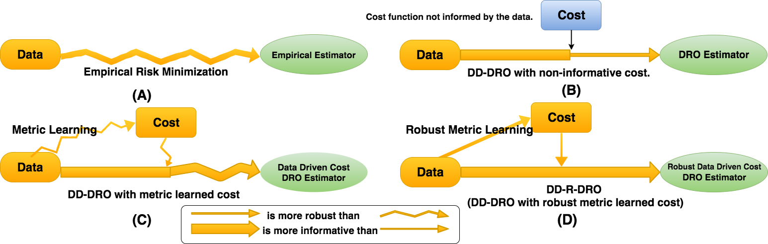
Figure 1. Four diagrams illustrating information on robustness.

Figure 1 shows the various combinations of information and robustness which have been studied in the literature so far. The figure shows four diagrams. Diagram (A) represents standard empirical risk minimization (ERM); which fully uses the information but often leads to high variability in testing error and, therefore, poor out-of-sample performance. Diagram (B) represents DD-DRO where only the center, $P_{n}$, and the size of the uncertainty, $\delta$, are data driven; this choice controls out-of-sample performance but does not use data to shape the type of perturbation, thus potentially resulting in testing error bounds which might be pessimistic. Diagram (C) represents DD-DRO with data-driven shape information for perturbation type using metric learning techniques; this construction can reduce the testing error bounds at the expense of increase in the variability of the testing error estimates. Diagram (D) represents DD-R-DRO, the shape of the perturbation allowed for the adversary player is estimated using an RO procedure; this double robustification, as we shall show in the numerical experiments is able to control the variability present in the third diagram.
In the diagrams, the straight arrows represent the use of a robustification procedure. A wide arrow represents the use of high degree of information. A wiggly arrow indicates potentially noisy testing error estimates.
The contributions of this paper can be stated, in order of importance, as follows:
1) The fourth diagram, DD-R-DRO, illustrates the main contribution of this paper, namely, a double robustification approach which reduces the generalization error, utilizes information efficiently, and controls variability.
2) An explicit RO formulation for metric learning tasks.
3) Iterative procedures for the solution of these RO problems.

2. DD-DRO, Optimal Transport, and Machine Learning

Let us consider a supervised machine learning classification problem, where we have a response $Y\in\{-1,1\}$ and predictors $X\in\mathbb{R}^{d}$. Underlying there is a general loss function $l(x,y,\beta)$ and a class of classifiers indexed by the parameter $\beta$. The distributional uncertainty region in (1) takes the form

(3) $$\mathcal{U}_{\delta}\left(P_{n}\right)=\left\{P:D_{c}\left(P,P_{n}\right)\leq\delta\right\},$$

where $D_{c}\left(P,P_{n}\right)$ is a suitably defined notion of discrepancy between $P$ and $P_{n}$ so that $D_{c}\left(P,P_{n}\right)=0$ implies that $P=P_{n}$.
Other notions of discrepancy have been considered in the DRO literaturem for example the Kullback-Leibler divergence (or another divergence notion which depends on the likelihood ratio) is utilized Hu and Hong, (2013). Unfortunately, divergence criteria which relies on the existence of the likelihood ratio between $P$ and $P_{n}$ ultimately forces $P$ to share the same support as $P_{n}$, therefore potentially inducing undesirable out-of-sample performance.
Instead, we follow the approach in Esfahani and Kuhn, (2015), Shafieezadeh-Abadeh et al., (2015), and Blanchet et al., (2016), and define $D_{c}\left(P,P_{n}\right)$ as the optimal transport discrepancy between $P$ and $P_{n}$.

2.1. Optimal Transport Distances and Discrepancies

Assume that the cost function $c:\mathbb{R}^{d+1}\times\mathbb{R}^{d+1}\rightarrow[0,\infty]$ is lower semicontinuous. We also assume that $c(u,v)=0$ if and only if $u=v$.
Given two distributions $P$ and $Q$, with supports $\mathcal{S}_{P}$ and $\mathcal{S}_{Q}$, respectively, we define the optimal transport discrepancy, $D_{c}$, via

(4) $$D_{c}\left(P,Q\right)=\inf\{E_{\pi}\left[c\left(U,V\right)\right]:\pi\in\mathcal{P}\left(\mathcal{S}_{P}\times\mathcal{S}_{Q}\right),\text{ }\pi_{U}=P,\text{ }\pi_{V}=Q\},$$

where $\mathcal{P}\left(\mathcal{S}_{P}\times\mathcal{S}_{Q}\right)$ is the set of probability distributions $\pi$ supported on $\mathcal{S}_{P}\times\mathcal{S}_{Q}$, and $\pi_{U}$ and $\pi_{V}$ denote the marginals of $U$ and $V$ under $\pi$, respectively. Because $c\left(\cdot\right)$ is non-negative we have that $D_{c}\left(P,Q\right)\geq 0$. Moreover, requiring that $c\left(u,v\right)=0$ if and only if $u=v$ guarantees that $D_{c}\left(P,Q\right)=0$ if and only $P=Q$.
If, in addition, $c\left(\cdot\right)$ is symmetric (i.e. $c\left(u,v\right)=c\left(v,u\right)$), and there exists $\varrho\geq 1$ such that $c^{1/\varrho}\left(u,w\right)\leq c^{1/\varrho}\left(u,v\right)+c^{1/\varrho}\left(v,w\right)$ (i.e. $c^{1/\varrho}\left(\cdot\right)$ satisfies the triangle inequality) then it can be easily verified (see Villani, (2008)) that $D_{c}^{1/\varrho}\left(P,Q\right)$ is a metric. For example, if $c\left(u,v\right)=\left\|u-v\right\|_{q}^{\varrho}$ for $q\geq 1$ (where $\left\|u-v\right\|_{q}$ denotes the $l_{q}$ norm in $\mathbb{R}^{d+1}$) then $D_{c}\left(\cdot\right)$ is known at the Wasserstein distance of order $\varrho$.
Observe that (4) is obtained by solving a linear programming problem. For example, suppose that $Q=P_{n}$, so $Q\in\mathcal{P}\left(\mathcal{D}_{n}\right)$ and assume that the support $\mathcal{S}_{P}$ of $P$ is finite. Then, using $U=\left(X,Y\right)$, we have that $D_{c}\left(P,P_{n}\right)$ is obtained by computing

(5) $$\min_{\pi}\sum_{u\in\mathcal{S}_{P}}\sum_{v\in\mathcal{D}_{n}}c\left(u,v\right)\pi\left(u,v\right):$$

s.t. $$\sum_{u\in\mathcal{S}_{P}}\pi\left(u,v\right)=\frac{1}{n}\text{ }\forall\text{ }v\in\mathcal{D}_{n}$$

$$\sum_{v\in\mathcal{D}_{N}}\pi\left(u,v\right)=P\left(\left\{u\right\}\right)\text{ }\forall\text{ }u\in\mathcal{X}_{N},$$

$$\pi\left(u,v\right)\geq 0\text{ }\forall\text{ }\left(u,v\right)\in\mathcal{S}_{P}\times\mathcal{D}_{n}$$

A completely analogous linear program (LP), albeit an infinite dimensional one, can be defined if $\mathcal{S}_{P}$ has infinitely many elements. This LP has been extensively studied in great generality in the context of Optimal Transport under the name of Kantorovich’s problem (see Villani, (2008))). Requiring $c\left(\cdot\right)$ to be lower semicontinuous guarantees the existence of an optimal solution to Kantorovich’s problem.
Note that $D_{c}\left(P,P_{n}\right)$ can be interpreted as the minimal cost of rearranging (i.e. transporting the mass of) the distribution $P_{n}$ into the distribution $P$. The rearrangement mechanism has a transportation cost $c\left(u,w\right)\geq 0$ for moving a unit of mass from location $u$ in the support of $P_{n}$ to location $w$ in the support of $P$. For instance, in the setting of (2) we have that

(6) $$c\left(\left(x,y\right),\left(x^{\prime},y^{\prime}\right)\right)=\left\|x-x^{\prime}\right\|_{q}^{2}I\left(y=y^{\prime}\right)+\infty\cdot I\left(y\neq y^{\prime}\right).$$

The infinite contribution in the definition of $c$ (i.e. $\infty\cdot I\left(y\neq y^{\prime}\right)$) indicates that the adversary player in the DRO formulation is not allowed to perturb the response variable.

3. Data-Driven Selection of Optimal Transport Cost Function

By suitably choosing $c\left(\cdot\right)$ we might further improve the generalization properties of the DD-DRO estimator based on (1). To fix ideas, consider a suitably parameterized family of transportation costs as follows. Let $\Lambda$ be a positive semidefinite matrix (denoted as $\Lambda\succeq 0$) and define $\left\|x\right\|_{\Lambda}^{2}=x^{T}\Lambda x$. Inspired by (6), consider the cost function

(7) $$c_{\Lambda}\left(\left(x,y\right),\left(x^{\prime},y^{\prime}\right)\right)=d_{\Lambda}^{2}\left(x,x^{\prime}\right)I\left(y=y^{\prime}\right)+\infty I\left(y\neq y^{\prime}\right),$$

where $d_{\Lambda}^{2}\left(x,x^{\prime}\right)=\left\|x-x^{\prime}\right\|_{\Lambda}^{2}$. Then, Blanchet et al., (2017) shows that in the generalized logistic regression setting (i.e. $l\left(x,y,\beta\right)=\log(1+\exp\left(-y\beta^{T}x\right))$), if $\Lambda$ is positive definite, we obtain

(8) $$\min_{\beta}\max_{P:D_{c_{\Lambda}}\left(P,P_{n}\right)\leq\delta}\mathbb{E}\left[l\left(X,Y,\beta\right)\right]=\min_{\beta}\mathbb{E}_{P_{n}}\left[l\left(X,Y,\beta\right)\right]+\delta\left\|\beta\right\|_{\Lambda^{-1}}.$$

If the choice of $\Lambda$ is data driven in order to impose a penalty on transportation costs whose outcomes that are highly impactful in terms of risk, then we would be able to control the risk bound induced by the DD-DRO formulation. This is the strategy studied in Blanchet et al., (2017) in which metric learning procedures have been implemented precisely to achieve such control. Our contribution, as we shall explain in the next section is the use of a robust optimization formulation to calibrate $c_{\Lambda}\left(\cdot\right)$. We emphasize that once $c_{\Lambda}\left(\cdot\right)$ is calibrated, it can be used to multiple learning tasks and arbitrary loss functions (not only logistic regression).

3.1. Data-Driven Cost Functions via Metric Learning Procedures

We quickly review the elements of standard metric learning procedures. Our data is of the form $\mathcal{D}_{n}=\left\{(X_{i},Y_{i})\right\}_{i=1}^{n}$ and $Y_{i}\in\{-1,+1\}$. The prediction variables are assumed to be standardized.
Motivated by applications such as social networks, in which there is a natural graph which can be used to connect instances in the data, we assume that one is given sets $\mathcal{M}$ and $\mathcal{N}$, where $\mathcal{M}$ is the set of the pairs that should be close (so that we can connect them) to each other, and $\mathcal{N}$, on contrary, is characterizing the relations that the pairs should be far away (not connected), we define them as

$$\mathcal{M} =\left\{\left(X_{i},X_{j}\right)|X_{i}\text{ and }X_{j}\text{ must connect}\right\},$$

$$\text{ and }\mathcal{N} =\left\{\left(X_{i},X_{j}\right)|X_{i}\text{ and }X_{j}\text{ should not connect}\right\}.$$

While it is typically assumed that $\mathcal{M}$ and $\mathcal{N}$ are given, one may always resort to $k$-Nearest-Neighbor ($k$-NN) method for the generation of these sets. This is the approach that we follow in our numerical experiments. But we emphasize that choosing any criterion for the definition of $\mathcal{M}$ and $\mathcal{N}$ should be influenced by the learning task in order to retain both interpretability and performance. In our experiments we let $\left(X_{i},X_{j}\right)$ belong to $\mathcal{M}$ if, in addition to being sufficiently close (i.e. in the $k$-NN criterion), $Y_{i}=Y_{j}$. If $Y_{i}\neq Y_{j}$, then we have that $\left(X_{i},X_{j}\right)\in\mathcal{N}$.
In addition, we consider the relative constraint set $\mathcal{R}$ containing data triplets with relative relation defined as

$$\mathcal{R}=\left\{\left(i,j,k\right)|d_{\Lambda}(X_{i},X_{j})\text{ should be smaller than }d_{\Lambda}(X_{i},X_{k})\right\}.$$

Let us consider the following two formulations of metric learning, the so-called Absolute Metric Learning formulation

(9) $$\min_{\Lambda\succeq 0}\sum_{\left(i,j\right)\in\mathcal{M}}d_{\Lambda}^{2}(X_{i},X_{j})\quad\text{s.t.}\quad\sum_{\left(i,j\right)\in\mathcal{N}}d_{A}^{2}(X_{i},X_{j})\geq 1,$$

and the Relative Metric Learning formulation,

(10) $$\min_{\Lambda\succeq 0}\sum_{\left(i,j,k\right)\in\mathcal{R}}\left(d_{\Lambda}^{2}\left(X_{i},X_{j}\right)-d_{\Lambda}^{2}\left(X_{i},X_{k}\right)+1\right)_{+}.$$

Both formulations have their merits, (9) exploits both the constraint sets $\mathcal{M}$ and $\mathcal{N}$, while (10) is only based on information in $\mathcal{R}$. Further intuition or motivation of those two formulations can be found in Xing et al., (2002) and Weinberger and Saul, (2009), respectively. We will show how to formulate and solve the robust counterpart of those two representative examples by robustifying a single constraint set or two sets simultaneously For simplicity we only discuss these two formulations, but many metric learning algorithms are based on natural generalizations of those two forms, as mentioned in the survey Bellet et al., (2013).
Once formulation (9) or (10) are considered and the matrix $\Lambda$ has been calibrated, one may then consider the cost function $c_{\Lambda}\left(\cdot\right)$ in (7) and solve the problem (8). This is the benchmark that we will consider in our numerical experiments. And we will contrast this approach versus a method which chooses $\Lambda$ using a robust optimization version of (9) or (10) as we shall explain next.

4. Robust Optimization for Metric Learning

In this section, we review a robust optimization method to metric learning optimization problem to learn a robust data-driven cost function. RO is a family of optimization techniques that deals with uncertainty or misspecification in the objective function and constraints. RO was first proposed in Ben-Tal et al., (2009) and has attracted increasing attentions in the recent decades El Ghaoui and Lebret, (1997) and Bertsimas et al., (2011). RO has been applied in machine learning to regularize statistical learning procedures, for example, in Xu et al., 2009a () and Xu et al., 2009b () robust optimization was employed for SR-Lasso and support vector machines. We apply RO, as we shall demonstrate, to reduce the variability in testing error when implementing DD-DRO.

4.1. Robust Optimization for Relative Metric Learning

The RO formulation that we shall use for (10) is based on the work of Huang et al., (2012). In order to motivate this formulation, suppose that we know that only $\alpha$ level, e.g. $\alpha=90\%$, of the constraints are satisfied, but we do not have information on exactly which of them are ultimately satisfied. The value of $\alpha$ may be inferred using cross validation.
Instead of optimizing over all subsets of constraints, we try to minimize the worst case loss function over all possible $\alpha\left|\mathcal{R}\right|$ constraints (where $\left|\cdot\right|$ is cardinality of a set) and obtain the following min-max formulation

(11) $$\min_{\Lambda\succeq 0}\max_{\tilde{q}\in\mathcal{T}(\alpha)}\sum_{(i,j,k)\in\mathcal{R}}q_{i,j,k}\left(d_{\Lambda}^{2}\left(X_{i},X_{j}\right)-d_{\Lambda}^{2}\left(X_{i},X_{k}\right)+1\right)_{+},$$

where $\mathcal{T}(\alpha)$ is a robust uncertainty set of the form

$$\mathcal{T}\left(\alpha\right)=\big{\{}\tilde{q}=\left\{q_{i,j,k}|(i,j,k)\in\mathcal{R}\right\}|0\leq q_{i,j,k}\leq 1,\sum_{(i,j,k)\in\mathcal{R}}q_{i,j,k}\leq\alpha\times\left|\mathcal{R}\right|\big{\}},$$

which is a convex and compact set.
In addition, the objective function in (10) is convex in $\Lambda$ and concave (linear) in $\tilde{q}$, so we can switch the order of min-max by resorting to Sion’s min-max theorem (Terkelsen, (1973)). This important observation suggests an iterative algorithm. For a fixed $\Lambda\succeq 0$, the inner maximization is linear in $\tilde{q}$, and the optimal $\tilde{q}$ satisfy $\tilde{q}_{i,j,k}=1$ whenever $\left(d_{\Lambda}\left(X_{i},X_{j}\right)-d_{\Lambda}\left(X_{i},X_{k}\right)+1\right)_{+}$ ranks in the top $\alpha\left|\mathcal{R}\right|$ largest values and equals $\tilde{q}_{i,j,k}$ otherwise.
Let us use $\mathcal{R}_{\alpha}\left(\Lambda\right)$ to denote the subset of constraints satisfying that the corresponding loss function $\left(d_{\Lambda}\left(X_{i},X_{j}\right)-d_{\Lambda}\left(X_{i},X_{k}\right)+1\right)_{+}$ ranks at the top $\alpha|\mathcal{R}|$ largest values among the corresponding loss function values of the triplets in $\mathcal{R}$.
For fixed $\tilde{q}$, the optimization problem is convex in $\Lambda$, we can solve this problem using sub-gradient or smoothing approximation algorithms (Nesterov, (2005)). Particularly, as we discussed above, if $\tilde{q}$ is the solution for fixed $\Lambda$, we know, solving $\Lambda$ is equivalent to solving its non-robust counterpart (10), replacing $\mathcal{R}$ by $\mathcal{R}_{\alpha}(\Lambda)$, where $\mathcal{R}_{\alpha}(\Lambda)$ is a subset of $\mathcal{R}$ that contains the constraints have top $\alpha|\mathcal{R}|$ violation, i.e.

$$\mathcal{R}_{\alpha}\left(\Lambda\right)=\left\{(i,j,k)\in\mathcal{R}|\left(d_{\Lambda}^{2}\left(X_{i},X_{j}\right)-d_{\Lambda}^{2}\left(X_{i},X_{k}\right)+1\right)_{+}\text{ ranks top }\alpha\text{ within }\mathcal{R}\right\}.$$

We summarize the sub-gradient based sequentially update algorithm as in Algorithm 1.

Algorithm 1 Sequential Coordinate-wise Metric Learning Using Relative Relations

1:Initialize $\Lambda=I_{d}$, learning rate $\alpha=0.01$ tracking error $Error=1000$ as a large number. Then randomly sample $\alpha$ proportion of elements from $\mathcal{R}$ to construct $\mathcal{R}_{\alpha}(\Lambda)$.

2:while $Error>10^{-3}$ do

3:     Update $\Lambda$ using projected (projected to positive semidefinite matrix cone) subgradient descent technique.

$$\Lambda=\pi_{\mathbb{S_{+}}}\big{(}\Lambda-\alpha\sum_{\left(i,j,k\right)\in\mathcal{R}_{\alpha}\left(\Lambda\right)}\nabla_{\Lambda}\left(d_{\Lambda}^{2}\left(X_{i},X_{j}\right)-d_{\Lambda}^{2}\left(X_{i},X_{k}\right)+1\right)_{+}\big{)}$$

4:     Update tracking error $Error$ as the norm of difference between latest matrix $\Lambda$ and average of last $50$ iterations.

5:     Every few steps (5 or 10 iterations), compute $\left(d_{\Lambda}^{2}\left(X_{i},X_{j}\right)-d_{\Lambda}^{2}\left(X_{i},X_{k}\right)+1\right)_{+}$ for all $\left(i,j,k\right)\in\mathcal{R}$, then update $\mathcal{R}_{\alpha}(\Lambda)$.

6:Output $\Lambda$.

As a remark, we would like to highlight the following observations. While we focus on metric learning simply as a loss minimization procedure as in (10) and (11) for simplicity, in practice people usually add a regularization term (such as $\left\|\Lambda\right\|_{F}$) to the loss minimization, as is common in metric learning literature (see Bellet et al., (2013)). It is easy to observe our discussion above regarding the min-max exchange uses Sion’s min-max theorem and everything else remains largely intact if we consider regularization. Likewise, one can use a more general loss functions than the hinge loss used in (10) and (11).

4.2. Robust Optimization for Absolute Metric Learning

The RO formulation that we present here for (9) appears to be novel in the literature. Note that (9) can be written into the Lagrangian form,

$$\min_{\Lambda\succeq 0}\quad\max_{\lambda\geq 0}\quad\sum_{\left(i,j\right)\in\mathcal{M}}d_{\Lambda}^{2}\left(X_{i},X_{j}\right)+\lambda\big{(}1-\sum_{\left(i,j\right)\in\mathcal{N}}d_{\Lambda}^{2}\left(X_{i},X_{j}\right)\big{)}.$$

Following similar discussion for $\mathcal{R}$, let us assume that the sets $\mathcal{M}$ and $\mathcal{N}$ are noisy or inaccurate at level $\alpha$ (i.e. $\alpha\cdot 100\%$ of their elements are incorrectly assigned). We can construct robust uncertainty sets $\mathcal{W}(\alpha)$ and $\mathcal{V}(\alpha)$ from the constraints in $\mathcal{M}$ and $\mathcal{N}$ as follows,

$$\mathcal{W}(\alpha) =\big{\{}\tilde{\eta}=\left\{\eta_{ij}:(i,j)\in\mathcal{M}\right\}|0\leq\eta_{ij}\leq 1,\sum_{(i,j)\in\mathcal{M}}\eta_{ij}\leq\alpha\times|\mathcal{M}|\big{\}},$$

$$\mathcal{V}(\alpha) =\big{\{}\tilde{\xi}=\left\{\xi_{ij}:(i,j)\in\mathcal{N}\right\}|0\leq\xi_{ij}\leq 1,\sum_{(i,j)\in\mathcal{N}}\xi_{ij}\geq\alpha\times|\mathcal{N}|\big{\}}.$$

Then we can write the RO counterpart for the loss minimization problem of metric learning as

(12) $$\min_{\Lambda\succeq 0}\quad\max_{\lambda\geq 0}\quad\max_{\tilde{\eta}\in\mathcal{W}(\alpha),\tilde{\xi}\in\mathcal{V}(\alpha)}\sum_{(i,j)\in\mathcal{M}}\eta_{i,j}d_{\Lambda}^{2}\left(X_{i},X_{j}\right)+\lambda\big{(}1-\sum_{(i,j)\in\mathcal{N}}\xi_{i,j}d_{\Lambda}^{2}\left(X_{i},X_{j}\right)\big{)}$$

Note that the Cartesian product $\mathcal{W}\left(\alpha\right)\times\mathcal{V}\left(\alpha\right)$ is a compact set, and the objective function is convex in $\Lambda$ and concave (linear) in pair $(\tilde{\eta},\tilde{\xi})$, so we can apply Sion’s min-max Theorem again (see in Terkelsen, (1973)) to switch the order of min_Λ-max${}_{(\tilde{\eta},\tilde{\xi})}$ (after switching max_λ and max${}_{(\tilde{\eta},\tilde{\xi})}$, which can be done in general). Then we can develop a sequential iterative algorithm to solve this problem as we describe next.
At the $k$-th step, given fixed $\Lambda_{k-1}\succeq 0$ and $\lambda_{k-1}>0$ (it is easy to observe that optimal solution $\lambda$ is positive, i.e. the constraint is active so we may safely assume $\lambda_{k-1}>0$), the inner maximization problem, becomes,

$$\max_{\tilde{\eta}\in\mathcal{W}\left(\alpha\right)}\sum_{(i,j)\in\mathcal{M}}\eta_{i,j}d_{\Lambda_{k-1}}^{2}\left(X_{i},X_{j}\right)+\lambda\big{(}1-\min_{\tilde{\xi}\in\mathcal{V}\left(\alpha\right)}\sum_{(i,j)\in\mathcal{N}}\xi_{i,j}d_{\Lambda_{k-1}}^{2}\left(X_{i},X_{j}\right)\big{)}.$$

As we discussed for relative constraints case, the optimal solution for $\tilde{\eta}$ and $\tilde{\xi}$ is, $\tilde{\eta}_{i,j}$ is 1, if $d_{\Lambda_{k-1}}^{2}\left(X_{i},X_{j}\right)$ ranks top $\alpha$ within $\mathcal{M}$ and equals 0 otherwise; while, on the contrary, $\tilde{\xi}_{i,j}=1$ if $d_{\Lambda_{k-1}}^{2}\left(X_{i},X_{j}\right)$ ranks bottom $\alpha$ within $\mathcal{N}$ and equals 0 otherwise.

Similar as $\mathcal{R}_{\alpha}(\Lambda)$, we can define $\mathcal{M}_{\alpha}(\Lambda_{k-1})$ ( $\mathcal{N}_{\alpha}(\Lambda_{k-1})$) as subset of $\mathcal{M}$ ($\mathcal{N}$), which contains the constraints with largest $\alpha$ percent of $d_{\Lambda_{k-1}}\left(\cdot\right)$ within in $\mathcal{M}$; and $\mathcal{N}_{\alpha}(\Lambda_{k-1})$ as subset of $\mathcal{N}$, which contains the constraints with smallest $\alpha$ percent of $d_{\Lambda_{k-1}}\left(\cdot\right)$ within in $\mathcal{N}$. As we observe that the optimal $\tilde{\eta}_{i,j}=1$ if $(i,j)\in\mathcal{M}_{\alpha}(\Lambda_{k-1})$ and $\tilde{\xi}_{i,j}=1$ if $(i,j)\in\mathcal{N}_{\alpha}(\Lambda_{k-1})$, thus for fixed $\tilde{\eta}$ and $\tilde{\xi}$, we can write the optimization problem over $\Lambda$ in the constrained case as

$$\min_{\Lambda\succeq 0}\quad\sum_{\left(i,j\right)\in\mathcal{M}_{\alpha}(\Lambda_{k-1})}d_{\Lambda}^{2}\left(X_{i},X_{j}\right)\quad\text{ s.t. }\quad\sum_{\left(i,j\right)\in\mathcal{N}_{\alpha}(\Lambda_{k-1})}d_{\Lambda}^{2}\left(X_{i},X_{j}\right)\geq 1.$$

This formulation falls within the setting of the problem stated in (9) and thus it can be solved by using techniques discussed in Xing et al., (2002). We summarize the details in Algorithm 2.

Algorithm 2 Sequential Coordinate-wise Metric Learning Using Absolute Constraints

1:Initialize $A=I_{d}$, tracking error $\text{Error}=1000$ as a large number. Then randomly sample $\alpha$ proportion of elements from $\mathcal{M}$ (resp. $\mathcal{N}$) to construct $\mathcal{M}_{\alpha}(A)$ (resp. $\mathcal{N}_{\alpha}(A)$).

2:while $Error>10^{-3}$ do

3:     Update $A$ using procedure provided in Xing et al., (2002).

4:     Update tracking error $Error$ as the norm of difference between latest matrix $A$ and average of last $50$ iterations.

5:     Every few steps (5 or 10 iterations), compute $d_{A}\left(W_{i},W_{j}\right)$ for all $\left(i,j\right)\in\mathcal{M}\cup\mathcal{N}$, then update $\mathcal{M}_{\alpha}(A)$ and $\mathcal{N}_{\alpha}(A)$.

6:Output $A$.

Other robust methods have also been considered in the metric learning literature, see Zha et al., (2009) and Lim et al., (2013) although the connections to RO are not fully exposed.

5. Numerical Experiments

We proceed to numerical experiments to verify the performance of our DD-R-DRO method empirically using six binary classification real data sets from UCI machine learning data base Lichman, (2013).
We consider logistic regression (LR), regularized logistic regression (LRL1), DD-DRO with cost function learned using absolute constraints (DD-DRO (absolute)) and its $\alpha=50\%,90\%$ level of doubly robust DRO (DD-R-DRO (absolute)); DD-DRO with cost function learned using relative constraints (DD-DRO (relative)) and its $\alpha=50\%,90\%$ level of doubly robust DRO (DD-R-DRO (relative)). For each data and each experiment, we randomly split the data into training and testing and fit models on training set and evaluate on testing set.
We report the mean and standard deviation of training error, testing error, and testing accuracy via $200$ independent experiments for each data sets, and summarize the detailed results and data set information (including split setting) in Table 1.
For solving the DD-DRO and DD-R-DRO problem, we apply the smoothing approximation algorithm introduced in Blanchet et al., (2017) to solve the DRO problem directly, where the size of uncertainty $\delta$ is chosen via $5-$fold cross-validation.

Table 1. Numerical results for real data sets.

		BC	BN	QSAR	Magic	MB	SB
LR	Train	$0\pm 0$	$.008\pm.003$	$.026\pm.008$	$.213\pm.153$	$0\pm 0$	$0\pm 0$
	Test	$8.75\pm 4.75$	$2.80\pm 1.44$	$35.5\pm 12.8$	$17.8\pm 6.77$	$18.2\pm 10.0$	$14.5\pm 9.04$
	Accur	$.762\pm.061$	$.926\pm.048$	$.701\pm.040$	$.668\pm.042$	$.678\pm.059$	$.789\pm.035$
LRL1	Train	$.185\pm.123$	$.080\pm.030$	$.614\pm.038$	$.548\pm.087$	$.401\pm.167$	$.470\pm.040$
	Test	$.428\pm.338$	$.340\pm.228$	$.755\pm.019$	$.610\pm.050$	$.910\pm.131$	$.588\pm.140$
	Accur	$.929\pm.023$	$.930\pm.042$	$.646\pm.036$	$.665\pm.045$	$.717\pm.041$	$.811\pm.034$
DD-DRO (absolute)	Train	$.022\pm.019$	$.197\pm.112$	$.402\pm.039$	$.469\pm.064$	$.294\pm.046$	$.166\pm.031$
	Test	$.126\pm.034$	$.275\pm.093$	$.557\pm.023$	$.571\pm.043$	$.613\pm.053$	$.333\pm.023$
	Accur	$.954\pm.015$	$.919\pm.050$	$.733\pm.0.026$	$.727\pm.039$	$.714\pm.032$	$.887\pm.011$
DD-R-DRO (absolute) $\alpha=90\%$	Train	$.029\pm.013$	$.078\pm.031$	$.397\pm.036$	$.420\pm.063$	$.249\pm.055$	$.194\pm.031$
	Test	$.126\pm.023$	$.259\pm.086$	$.554\pm.019$	$.561\pm.035$	$.609\pm.044$	$.331\pm.018$
	Accur	$.954\pm.012$	$.910\pm.042$	$.736\pm.025$	$.729\pm.032$	$.709\pm.025$	$.890\pm.008$
DD-R-DRO (absolute) $\alpha=50\%$	Train	$.040\pm.055$	$.137\pm.030$	$.448\pm.032$	$.504\pm.041$	$.351\pm.048$	$.166\pm.030$
	Test	$.132\pm.015$	$.288\pm.059$	$.579\pm.017$	$.590\pm.029$	$.623\pm.029$	$.337\pm.013$
	Accur	$.952\pm.012$	$.918\pm.037$	$.733\pm.025$	$.710\pm.033$	$.715\pm.021$	$.888\pm.008$
DD-DRO (relative)	Train	$.086\pm.038$	$.436\pm.138$	$.392\pm.040$	$.457\pm.071$	$.322\pm.061$	$.181\pm,036$
	Test	$.153\pm.060$	$.329\pm.124$	$.559\pm.025$	$582\pm.033$	$.613\pm.031$	$.332\pm.016$
	Accur	$.946\pm.018$	$.916\pm.075$	$.714\pm.029$	$.710\pm,027$	$.704\pm.021$	$.890\pm.008$
DD-R-DRO (relative) $\alpha=90\%$	Train	$.030\pm.014$	$.244\pm.121$	$.375\pm.038$	$.452\pm.067$	$.402\pm.058$	$.234\pm.032$
	Test	$.141\pm.054$	$.300\pm$.108	$.556\pm.022$	$.577\pm.032$	$.610\pm.024$	$.332\pm.011$
	Accur	$.949\pm.019$	$.921\pm.070$	$.729\pm.023$	$.717\pm.025$	$.710\pm.020$	$.892\pm.007$
DD-R-DRO (relative) $\alpha=50\%$	Train	$.031\pm.016$	$.232\pm.094$	$.445\pm.032$	$.544\pm.057$	$.365\pm.054$	$.288\pm.029$
	Test	$.154\pm.049$	$.319\pm.078$	$.570\pm.019$	$.594\pm.018$	$.624\pm.018$	$.357\pm.008$
	Accur	$.948\pm.019$	$.918\pm.081$	$.705\pm.023$	$.699\pm.028$	$.698\pm.018$	$.881\pm.005$
Num Predictors		$30$	$4$	$30$	$10$	$20$	$56$
Train Size		$40$	$20$	$80$	$30$	$30$	$150$
Test Size		$329$	$752$	$475$	$9990$	$125034$	$2951$

We observe that the doubly robust DRO framework, in general, get robust improvement comparing to its non-robust counterpart with $\alpha=90\%$. More importantly, the robust methods tend to enjoy the variance reduction property due to RO. Also, as the robust level increases, i.e. $\alpha=50\%$, where we believe in higher noise in cost function learning, we can observe, the doubly robust based approach seems to shrink towards to LRL1, and benefits less from the data-driven cost structure.

6. Discussion and Conclusion

We have proposed a novel methodology, DD-R-DRO, which calibrates a transportation cost function by using a data-driven approach based on RO. In turn, DD-R-DRO uses this cost function in the description of a DRO formulation based on optimal transport uncertainty region. The overall methodology is doubly robust. On one hand, DD-DRO, which fully uses the training data to estimate the underlying transportation cost enhances out-of-sample performance by allowing an adversary to perturb the data (represented by the empirical distribution) in order to obtain bounds on the testing risk which are tight. On the other hand, the tightness of bounds might come at the cost of potentially introducing noise in the testing error performance. The second layer of robustification, as shown in the numerical examples, mitigates precisely the presence of this noise.

References

- Bellet et al., [2013] Bellet, A., Habrard, A., and Sebban, M. (2013). A survey on metric learning for feature vectors and structured data. arXiv preprint arXiv:1306.6709.
- Ben-Tal et al., [2009] Ben-Tal, A., El Ghaoui, L., and Nemirovski, A. (2009). Robust optimization. Princeton University Press.
- Bertsimas et al., [2011] Bertsimas, D., Brown, D. B., and Caramanis, C. (2011). Theory and applications of robust optimization. SIAM review, 53(3):464–501.
- Blanchet et al., [2016] Blanchet, J., Kang, Y., and Murthy, K. (2016). Robust wasserstein profile inference and applications to machine learning. arXiv preprint arXiv:1610.05627.
- Blanchet et al., [2017] Blanchet, J., Kang, Y., Zhang, F., and Murthy, K. (2017). Data-driven optimal transport cost selection for distributionally robust optimization. arXiv preprint arXiv:.
- El Ghaoui and Lebret, [1997] El Ghaoui, L. and Lebret, H. (1997). Robust solutions to least-squares problems with uncertain data. SIAM Journal on Matrix Analysis and Applications, 18(4):1035–1064.
- Esfahani and Kuhn, [2015] Esfahani, P. M. and Kuhn, D. (2015). Data-driven distributionally robust optimization using the wasserstein metric: Performance guarantees and tractable reformulations. arXiv preprint arXiv:1505.05116.
- Hu and Hong, [2013] Hu, Z. and Hong, L. J. (2013). Kullback-leibler divergence constrained distributionally robust optimization. Available at Optimization Online.
- Huang et al., [2012] Huang, K., Jin, R., Xu, Z., and Liu, C.-L. (2012). Robust metric learning by smooth optimization. arXiv preprint arXiv:1203.3461.
- Lichman, [2013] Lichman, M. (2013). UCI machine learning repository.
- Lim et al., [2013] Lim, D., McFee, B., and Lanckriet, G. R. (2013). Robust structural metric learning. In ICML-13, pages 615–623.
- Nesterov, [2005] Nesterov, Y. (2005). Smooth minimization of non-smooth functions. Mathematical programming, 103(1):127–152.
- Shafieezadeh-Abadeh et al., [2015] Shafieezadeh-Abadeh, S., Esfahani, P. M., and Kuhn, D. (2015). Distributionally robust logistic regression. In Advances in Neural Information Processing Systems, pages 1576–1584.
- Terkelsen, [1973] Terkelsen, F. (1973). Some minimax theorems. Mathematica Scandinavica, 31(2):405–413.
- Villani, [2008] Villani, C. (2008). Optimal transport: old and new, volume 338. Springer Science & Business Media.
- Weinberger and Saul, [2009] Weinberger, K. Q. and Saul, L. K. (2009). Distance metric learning for large margin nearest neighbor classification. JMLR, 10(Feb):207–244.
- Xing et al., [2002] Xing, E. P., Ng, A. Y., Jordan, M. I., and Russell, S. (2002). Distance metric learning with application to clustering with side-information. In NIPS-2002, volume 15, page 12.
- [18] Xu, H., Caramanis, C., and Mannor, S. (2009a). Robust regression and lasso. In NIPS-2009, pages 1801–1808.
- [19] Xu, H., Caramanis, C., and Mannor, S. (2009b). Robustness and regularization of support vector machines. JMLR, 10(Jul):1485–1510.
- Zha et al., [2009] Zha, Z.-J., Mei, T., Wang, M., Wang, Z., and Hua, X.-S. (2009). Robust distance metric learning with auxiliary knowledge. In IJCAI, pages 1327–1332.