Connecting Different TMD Factorization Formalisms in QCD

Abstract

In the original Collins-Soper-Sterman (CSS) presentation of the results of transverse-momentum-dependent (TMD) factorization for the Drell-Yan process, results for perturbative coefficients can be obtained from calculations for collinear factorization. Here we show how to use these results, plus known results for the quark form factor, to obtain coefficients for TMD factorization in more recent formulations, e.g., that due to Collins, and apply them to known results at order $\alpha_{s}^{2}$ and $\alpha_{s}^{3}$. We also show that the “non-perturbative” functions as obtained from fits to data are equal in the two schemes. We compile the higher-order perturbative inputs needed for the updated CSS scheme by appealing to results obtained in a variety of different formalisms. In addition, we derive the connection between both versions of the CSS formalism and several formalisms based in soft-collinear effective theory (SCET). Our work uses some important new results for factorization for the quark form factor, which we derive.

I Introduction

In the application of transverse-momentum-dependent (TMD) factorization to the Drell-Yan and other processes, many standard fits to data, like those of Refs. Landry et al. (2003); Konychev and Nadolsky (2006), use a presentation of a TMD factorization formula due to Collins, Soper, and Sterman (CSS1) Collins et al. (1985). In this method, the cross section is written as a Fourier transform over a transverse-position variable $\boldsymbol{b}_{\text{T}}$. The $\boldsymbol{b}_{\text{T}}$ dependence is separated into a part estimated by perturbative methods, and a correction factor involving certain functions $g_{K}(b_{\text{T}})$, $g_{j/H}(x,b_{\text{T}})$ that allow for a parametrization of the important non-perturbative dependence at large $b_{\text{T}}$. The perturbative part is restricted to use $b_{\text{T}}$ less than a cut-off $b_{\rm max}$. Results of fits are presented as parametrizations for the “non-perturbative” functions $g_{K}(b_{\text{T}})$, $g_{j/H}(x,b_{\text{T}}{})$ etc. (Let us call these collectively the “$g$-functions.”)

Two issues now arise. The first is that an improved version of TMD factorization has been derived in Ref. Collins (2011), and that some closely related formalisms have been developed within the framework of soft-collinear effective theory (SCET). Let us refer to the version in Ref. Collins (2011) as CSS2.

The second issue is that the fitted functions, the $g$-functions, are not intrinsically interpretable in terms of TMD parton densities, but only in conjunction with the cut-off-dependent perturbative part of the factorization formula. This raises questions about the validity of using $g$-functions extracted using one perturbative formalism for calculations and phenomenology in another formalism. Aybat and Rogers (2011) already organized the TMD functions in accordance with the new definitions, and used existing previously existing phenomenology to construct TMD parametrizations of parton densities in terms of $g$-functions. However, until now it has not been firmly established that the $g$-functions extracted using the older CSS1 formalism actually apply directly to the TMD functions defined in CSS2.

In this article we therefore do the following: We show how to relate the two versions of the CSS-style formalism, so that results of fits obtained using the original CSS factorization formula can be applied in the new formalism. We also derive explicit transformations to implement the scheme change between the two formalisms. Key quantities in both formalisms are TMD parton densities and the CSS evolution kernel $\tilde{K}(b_{\text{T}})$, which are defined in terms of certain QCD matrix elements. The present article’s advances include obtaining the full relations between the old and new schemes, showing completely how fits made using the old scheme can be applied to give TMD parton densities in the new scheme. We show that the $g$-functions in the two schemes are equal. We give formulae for the TMD functions with the new definitions in terms of the fitted functions obtained using the original CSS formalism. The resulting TMD functions have an invariant significance, independently of the details of the specific implementation and of values of arbitrary perturbative cutoffs like the renormalization scale and the $b_{\rm max}$ cut off.

We compute various functions needed in the formalism, on the basis of existing calculations of the quark form factor by Moch et al. (2005), and of hard scattering in collinear factorization by Catani et al. (2001). These results are: (a) The coefficients relating TMD and collinear parton densities to order $a_{s}^{2}$; (b) The TMD hard scattering coefficient for Drell-Yan to order $a_{s}^{2}$; (c) The anomalous dimensions to order $a_{s}^{3}$; (d) The CSS2 evolution kernel $\tilde{K}$ to order $a_{s}^{2}$. We give full details of the non-trivial methods by which the coefficients are obtained from the previous results. In particular we find that we need some apparently new technical results concerning the collinear factors used for factorization for the quark form factor. We verify that our results agree with calculations of corresponding quantities by very different methods by Gehrmann et al. (2012, 2014) and by Echevarria et al. (2016). Those calculations start from the operator definitions of the TMD functions, and so the agreement with our calculations provides a non-trivial test of the correctness of the TMD factorization methods. We point out that the order $a_{s}^{3}$ value for the hard scattering is available from results by Gehrmann et al. (2010), and that a calculation by Li and Zhu (2017) gives the value of $\tilde{K}$ to order $a_{s}^{3}$. That the result of Ref. Li and Zhu (2017) in fact gives exactly the perturbative expansion of $\tilde{K}$ is not immediately apparent from their paper, so we give a derivation of the correspondence in App. B, where we also show how to map their factorization and TMD parton densities onto those given by CSS2 and by Echevarría et al. (2012).

II The formalisms

II.1 Notation and conventions

To match the conventions of Moch et al. (2005), we use

$$a_{s}=\frac{\alpha_{s}}{4\pi}=\frac{g_{s}^{2}}{16\pi^{2}}$$ (1)

as the expansion parameter.

II.2 Original CSS formalism

The original CSS formula (Collins et al., 1985, (3.17) and (5.8)), as used in the fits in Landry et al. (2003); Konychev and Nadolsky (2006), was obtained starting from a TMD factorization formula, using the specific definitions of TMD parton densities that had been given by Collins and Soper (CS) Collins and Soper (1982a). Earlier, CS Collins and Soper (1981, 1982b) had obtained TMD factorization for dihadron production in $e^{+}e^{-}$ annihilation. The natural extension to the Drell-Yan process was stated by CSS in Collins et al. (1985); CSS argued that the then-recent work on the cancellation of the Glauber region was sufficient to allow the extension of the proof of TMD factorization to Drell-Yan.

Associated with factorization are evolution equations for the TMD functions and a kind of operator-product expansion (OPE) for the TMD parton densities at small $b_{\text{T}}$. CSS solved these equations with neglect of power-suppressed terms, segregated non-perturbative contributions at large $b_{\text{T}}$, and then redefined various functions. The result was of the form

$$\frac{\mathop{\mathrm{d}\mskip-0.59999mu\sigma}\nolimits}{\mathop{\mathrm{d}\mskip-0.59999muQ^{2}}\nolimits\mathop{\mathrm{d}\mskip-0.59999muy}\nolimits\mathop{\mathrm{d}\mskip-0.59999muq_{\text{T}}^{2}}\nolimits}={} \frac{4\pi^{2}\alpha^{2}}{9Q^{2}s}\sum_{j,j_{A},j_{B}}e_{j}^{2}\int\frac{\mathop{\mathrm{d}^{2}\mskip-0.59999mu\boldsymbol{b}_{\text{T}}}\nolimits}{(2\pi)^{2}}e^{i\boldsymbol{q}_{\text{T}}\cdot\boldsymbol{b}_{\text{T}}}$$

$$\times\int_{x_{A}}^{1}\frac{\mathop{\mathrm{d}\mskip-0.59999mu\xi_{A}}\nolimits}{\xi_{A}}f_{j_{A}/A}(\xi_{A};\mu_{b_{*}})~{}\tilde{C}^{\text{CSS1, DY}}_{j/j_{A}}\mathopen{}\left(\frac{x_{A}}{\xi_{A}},b_{*};\mu_{b_{*}}^{2},\mu_{b_{*}},C_{2},a_{s}(\mu_{b_{*}})\right)$$

$$\times\int_{x_{B}}^{1}\frac{\mathop{\mathrm{d}\mskip-0.59999mu\xi_{B}}\nolimits}{\xi_{B}}f_{j_{B}/B}(\xi_{B};\mu_{b_{*}})~{}\tilde{C}^{\text{CSS1, DY}}_{\bar{\jmath}/j_{B}}\mathopen{}\left(\frac{x_{B}}{\xi_{B}},b_{*};\mu_{b_{*}}^{2},\mu_{b_{*}},C_{2},a_{s}(\mu_{b_{*}})\right)$$

$$\times\exp\left\{-\int_{\mu_{b_{*}}^{2}}^{\mu_{Q}^{2}}\frac{\mathop{\mathrm{d}\mskip-0.59999mu{\mu^{\prime}}^{2}}\nolimits}{{\mu^{\prime}}^{2}}\left[A_{\rm CSS1}(a_{s}(\mu^{\prime});C_{1})\ln\left(\frac{\mu_{Q}^{2}}{{\mu^{\prime}}^{2}}\right)+B_{\text{CSS1, DY}}(a_{s}(\mu^{\prime});C_{1},C_{2})\right]\right\}$$

$$\times\exp\mathopen{}\left[-g^{\rm CSS1}_{j/A}(x_{A},b_{\text{T}};b_{\rm max})-g^{\rm CSS1}_{\bar{\jmath}/B}(x_{B},b_{\text{T}};b_{\rm max})-g^{\rm CSS1}_{K}(b_{\text{T}};b_{\rm max})\ln(Q^{2}/Q_{0}^{2})\right]$$

$$+\mbox{suppressed corrections}.$$ (2)

Here we work with the inclusive Drell-Yan process $A+B\to l^{+}l^{-}+X$, with restriction to production of the lepton pair through a virtual photon. The 4-momentum of the lepton pair is $q^{\mu}$, and its invariant mass, rapidity and transverse momentum are $Q$, $y$ and $\boldsymbol{q}_{\text{T}}$. The total center of mass energy is $\sqrt{s}$, we define $x_{A}=Qe^{y}/\sqrt{s}$ and $x_{B}=Qe^{-y}/\sqrt{s}$, we define $e_{j}$ to be the charge of quark $j$ (in units of the elementary charge unit $e$), and $\alpha$ is the usual fine-structure constant. Auxiliary quantities are defined by

$$\boldsymbol{b}_{*} =\frac{\boldsymbol{b}_{\text{T}}}{\sqrt{1+b_{\text{T}}^{2}/b_{\rm max}^{2}}},$$ (3)

$$\mu_{b_{*}} =C_{1}/b_{*},$$ (4)

$$\mu_{Q} =C_{2}Q,$$ (5)

with $C_{1}$ and $C_{2}$ being constants that can be adjusted to try to optimize the accuracy of perturbative calculations; if all quantities were computed exactly, the results of predictions would be independent of $C_{1}$ and $C_{2}$. The quantities $f_{j/H}$ are ordinary collinear parton densities (in the $\overline{\rm MS}$ scheme, normally). Those quantities that are specific to the particular definitions given by CSS are indicated with the label “CSS1”. The functions $A_{\rm CSS1}$, $B_{\text{CSS1, DY}}$, and $\tilde{C}^{\text{CSS1, DY}}$ are perturbatively calculable. Corrections to the formula, as noted on the last line, are power suppressed when $Q$ is large and $q_{\text{T}}\ll Q$. We will ignore various polarization-related effects that have considerable current interest (e.g., Ref. Adolph et al. (2015); Aubert et al. (2015); Ablikim et al. (2016)) but that do not directly intersect with the issues that are the main concern of this article; our results can be straightforwardly extended to the case of polarization dependent observables.

The derivation of (II.2) from the underlying TMD factorization formula used a certain set of redefinitions Collins and Soper (1982b); Collins et al. (1985) of various parts of the factorization formula. An important motivation was to express the cross section in terms of quantities that can be related to experimental data. For example, in the initial CSS1 factorization formula there is a soft factor. This has non-perturbative contributions but always appears multiplying a pair of TMD parton densities or fragmentation functions. Thus, the non-perturbative part of the soft factor cannot be separately and unambiguously deduced from data, even in principle. A properly defined soft factor is universal between reactions (Collins, 2011, Ch. 13). So absorbing a square root of the soft factor into each parton density and fragmentation function is sensible.

Having separate and explicitly defined TMD pdf definitions also opens the possibility to study such objects non-perturbatively, e.g., with lattice QCD Engelhardt et al. (2016).

But CSS1 also absorbed a square root of a hard factor into the parton densities and fragmentation functions. This is much less desirable, since these functions then become process dependent—see Catani et al. (2001) and (Collins and Soper, 1982b, p. 455). The hard scattering is always perturbatively calculable (and hence predictable), so the CSS1 procedure obscures the predictable differences between processes.

The new method of CSS2, reviewed in the next section, is better from this point of view.

II.3 New TMD formalism

Collins (2011, Chs. 10 & 13) provided an updated TMD factorization. Much more complete derivations were provided. Relative to CSS1, the most notable change is a modified definition of the TMD parton densities and fragmentation functions, in terms of explicit gauge-invariant operator matrix elements. The new definitions have as a consequence that the TMD factorization formula no longer contains an explicit soft factor. Furthermore, the definitions were arranged so that the evolution equations are exact in their form, instead of having power-suppressed corrections; this makes the relation between the results of fits and the actual TMD parton densities much more transparent.

The TMD functions, with their new definitions, are demonstrably process independent, up to possible sign changes associated with T-odd functions. In the factorization formula, only the perturbatively calculable hard scattering contains process dependence. The method also avoids the divergences that were found by Bacchetta et al. (2008, App. A) when the original CS definition of TMD densities is taken literally.

Despite these changes, the new method should be considered a scheme change relative the original CS/CSS definitions, as we will see in later sections.

A summary of the new method can be found in Collins and Rogers (2015), together with a set of different forms of solution. Here, we will present only those results needed for our purposes, but adapted to the cross section given in Eq. (II.2).

Within the framework of SCET, closely related TMD factorization results have been given by Becher and Neubert (2011) and by Echevarría et al. (2012). The results of Echevarría et al. are equivalent Collins and Rogers (2013) to those presented here, with the TMD functions being the same (up to possible elementary changes in the scheme used for UV renormalization); their formula defining the TMD densities is simpler than that of Ref. Collins (2011). Becher and Neubert did not define separately finite TMD functions. But they did define the product of two such functions, as used in factorization formulae, and the product agrees with the product of the TMD functions used here and by Echevarría et al. (Details of this can be extracted from a comparison of the relevant formulae in Becher and Neubert (2011); Echevarría et al. (2012); Collins and Rogers (2013).) There is also the formulation of TMD factorization given by Li et al. (2016), which looks rather different. We will show in App. B how it can be mapped, non-trivially, onto the CSS2 formalism; the result will enable use in CSS2 of the order $a_{s}^{3}$ calculations of the evolution of the soft factor that were given by Li and Zhu (2017).

The TMD factorization formula is

$$\frac{\mathop{\mathrm{d}\mskip-0.59999mu\sigma}\nolimits}{\mathop{\mathrm{d}\mskip-0.59999muQ^{2}}\nolimits\mathop{\mathrm{d}\mskip-0.59999muy}\nolimits\mathop{\mathrm{d}\mskip-0.59999muq_{\text{T}}^{2}}\nolimits}={} \frac{4\pi^{2}\alpha^{2}}{9Q^{2}s}\sum_{j}H^{\rm DY}_{j\bar{\jmath}}(Q,\mu_{Q},a_{s}(\mu_{Q}))\int\frac{\mathop{\mathrm{d}^{2}\mskip-0.59999mu\boldsymbol{b}_{\text{T}}}\nolimits}{(2\pi)^{2}}~{}e^{i\boldsymbol{q}_{\text{T}}\cdot\boldsymbol{b}_{\text{T}}}~{}\tilde{f}_{j/A}(x_{A},b_{\text{T}};Q^{2},\mu_{Q})~{}\tilde{f}_{\bar{\jmath}/B}(x_{B},b_{\text{T}};Q^{2},\mu_{Q})$$

$$+\mbox{suppressed corrections},$$ (6)

where the hard scattering factor $H^{\rm DY}_{j\bar{\jmath}}$ is normalized so that its lowest order term is $e_{j}^{2}$. The scale argument of $H$ is set to $\mu_{Q}$ to avoid large logarithms. The last two arguments of the parton densities, $f_{j/H}(x,b_{\text{T}};Q^{2},\mu_{Q})$, are normally written as $\zeta$ and $\mu$, and these arguments refer to effective cutoffs on rapidity and transverse momentum as implemented by the definitions in Collins (2011).

Predictions are obtained with the aid of evolution equations and the small-$b_{\text{T}}$ OPE of the TMD parton densities:

$$\frac{\partial\ln\tilde{f}_{f/H}(x,b_{\text{T}};\zeta;\mu)}{\partial\ln\sqrt{\zeta}}={} \tilde{K}(b_{\text{T}};\mu).$$ (7)

$$\frac{\mathop{\mathrm{d}\mskip-0.59999mu\tilde{K}(b_{\text{T}};\mu)}\nolimits}{\mathop{\mathrm{d}\mskip-0.59999mu\ln\mu}\nolimits}={} -\gamma_{K}\mathopen{}\left(a_{s}(\mu)\right),$$ (8)

$$\frac{\mathop{\mathrm{d}\mskip-0.59999mu\ln\tilde{f}_{j/H}(x,b_{\text{T}};\zeta;\mu)}\nolimits}{\mathop{\mathrm{d}\mskip-0.59999mu\ln\mu}\nolimits}={} \gamma_{j}(a_{s}(\mu))-\frac{1}{2}\gamma_{K}(a_{s}(\mu))\ln\frac{\zeta}{\mu^{2}},$$ (9)

$$\tilde{f}_{j/H}(x,b_{\text{T}};\zeta;\mu)={} \sum_{k}\int_{x-}^{1+}\frac{\mathop{\mathrm{d}\mskip-0.59999mu\xi}\nolimits}{\xi}\,\tilde{C}^{\rm PDF}_{j/k}\mathopen{}\left(x/\xi,b_{\text{T}};\zeta,\mu,a_{s}(\mu)\right)f_{k/H}(\xi;\mu)~{}+~{}O\mathopen{}\left[(mb_{\text{T}})^{p}\right].$$ (10)

(For an explanation of the notations $x-$ and $1+$ for the integration limits, see (Collins, 2011, pp. 248 & 249).) A solution that corresponds to Eq. (II.2) is

$$\frac{\mathop{\mathrm{d}\mskip-0.59999mu\sigma}\nolimits}{\mathop{\mathrm{d}\mskip-0.59999muQ^{2}}\nolimits\mathop{\mathrm{d}\mskip-0.59999muy}\nolimits\mathop{\mathrm{d}\mskip-0.59999muq_{\text{T}}^{2}}\nolimits}={} \frac{4\pi^{2}\alpha^{2}}{9Q^{2}s}\sum_{j,j_{A},j_{B}}H^{\rm DY}_{j\bar{\jmath}}(Q,\mu_{Q},a_{s}(\mu_{Q}))\int\frac{\mathop{\mathrm{d}^{2}\mskip-0.59999mu\boldsymbol{b}_{\text{T}}}\nolimits}{(2\pi)^{2}}e^{i\boldsymbol{q}_{\text{T}}\cdot\boldsymbol{b}_{\text{T}}}$$

$$~{}~{}\times e^{-g_{j/A}(x_{A},b_{\text{T}};b_{\rm max})}\int_{x_{A}}^{1}\frac{\mathop{\mathrm{d}\mskip-0.59999mu\xi_{A}}\nolimits}{\xi_{A}}f_{j_{A}/A}(\xi_{A};\mu_{b_{*}})~{}\tilde{C}^{\rm PDF}_{j/j_{A}}\mathopen{}\left(\frac{x_{A}}{\xi_{A}},b_{*};\mu_{b_{*}}^{2},\mu_{b_{*}},a_{s}(\mu_{b_{*}})\right)$$

$$~{}~{}\times e^{-g_{\bar{\jmath}/B}(x_{B},b_{\text{T}};b_{\rm max})}\int_{x_{B}}^{1}\frac{\mathop{\mathrm{d}\mskip-0.59999mu\xi_{B}}\nolimits}{\xi_{B}}f_{j_{B}/B}(\xi_{B};\mu_{b_{*}})~{}\tilde{C}^{\rm PDF}_{\bar{\jmath}/j_{B}}\mathopen{}\left(\frac{x_{B}}{\xi_{B}},b_{*};\mu_{b_{*}}^{2},\mu_{b_{*}},a_{s}(\mu_{b_{*}})\right)$$

$$~{}~{}\times\exp\mathopen{}\left\{-g_{K}(b_{\text{T}};b_{\rm max})\ln\frac{Q^{2}}{Q_{0}^{2}}+\tilde{K}(b_{*};\mu_{b_{*}})\ln\frac{Q^{2}}{\mu_{b_{*}}^{2}}+\int_{\mu_{b_{*}}}^{\mu_{Q}}\frac{\mathop{\mathrm{d}\mskip-0.59999mu\mu^{\prime}}\nolimits}{\mu^{\prime}}\left[2\gamma_{j}(a_{s}(\mu^{\prime}))-\ln\frac{Q^{2}}{(\mu^{\prime})^{2}}\gamma_{K}(a_{s}(\mu^{\prime}))\right]\right\}$$

$$+\mbox{suppressed corrections}.$$ (11)

Analogous equations apply to fragmentation functions in processes like semi-inclusive deeply inelastic scattering (SIDIS) and $e^{+}e^{-}$ annihilation, with the same $\tilde{K}$, $\gamma_{j}$, and $\gamma_{K}$ functions. (Equality of $\tilde{K}$ and $\gamma_{K}$ between the processes was proved in Ref. Collins (2011); equality of $\gamma_{j}$ will be proved in our Sec. VII.) Note the ${\rm DY}$ label on the hard part, $H_{j\bar{\jmath}}^{\rm DY}(Q,\mu_{Q},a_{s}(\mu_{Q}))$, to indicate that this hard part is specific to the Drell-Yan scattering process. We have used the notation $\tilde{C}^{\rm PDF}$ to indicate that the corresponding coefficients will be different for fragmentation functions.

II.4 The mismatches between CSS1 and the new methods

In all the methods, the primary idea is to extract the leading power behavior in an expansion where masses and $q_{\text{T}}{}$ are small relative to $Q$. By far the simplest form of the results for factorization is when the leading-power expansion is used strictly; terms of non-leading power tend to be more complicated. A problem is that when a strict leading power expansion is done, one obtains individual terms that have UV and rapidity divergences not present in the original amplitudes. So at intermediate stages of derivations and calculations, cutoffs (or regulators) are applied to the divergences. All the methods are in agreement to deal with UV divergences by renormalization, after which the UV cutoff can be removed. The differences between the methods concern the treatment of rapidity divergences.

The rapidity divergences are associated with the light-like Wilson lines that arise when the operators in the factors are defined in the natural gauge-invariant way that arises from the leading-power expansion, or some equivalent property.

In CSS1, collinear factors are defined with the use of a non-light-like axial gauge, or equivalently with non-lightlike Wilson lines. For example, in the case of the quark form factor, the collinear factor would be defined by the matrix element in Eq. (100) below, but without the limit $y_{2}\to-\infty$ (and the $S$ factors are moved elsewhere). Effectively some non-leading powers are retained. Correspondingly, the evolution equations have power corrections; these were not analyzed by CSS, and instead the corrections are dropped in a solution such as Eq. (II.2). Thus there is a mismatch between the actual TMD pdfs defined in Ref. Collins and Soper (1982a) and those that correspond to Eq. (II.2), although the differences are power suppressed.

Furthermore, in CSS1 the TMD factors were then redefined to remove the hard factor and soft factor that would otherwise be present; this produces the process dependence of the TMD parton densities and fragmentation functions that was mentioned earlier.

In CSS2 and the SCET methods we have quoted, a strict leading power expansion is used. Although cutoffs on rapidity divergences are used at intermediate stages, these are removed at the end. Thus the basic collinear and soft factors have the lightlike Wilson lines that naturally arise from a gauge-invariant implementation of the leading power expansion. There are then applied certain kinds of reorganization of the factors and/or a generalized renormalization of the rapidity divergences. These both avoid double counting of the contributions of different regions and ensure that individual TMD functions used in factorization are finite.

In CSS2 itself, there remain non-lightlike Wilson lines, as in Eq. (100) below. But these are always in matrix elements of a basic soft factor where the other Wilson line is lightlike. The dependence of a collinear factor on the direction of this Wilson line gives the $\zeta$ dependence of the TMD functions. In contrast in the SCET methods, especially that of Echevarría et al. (2012), the Wilson lines are always lightlike, and another regulator is used. The role of the direction of CSS2’s non-lightlike Wilson line is now played by a choice of coordination between the regulator of oppositely directed Wilson lines; it gives rise to the same $\zeta$ dependence Collins and Rogers (2013). The final factorization formula and the TMD functions are defined in the limit that the regulators are removed. The factorization formula then has exactly the leading power, and the evolution equations are homogeneous without any power-suppressed corrections.

III New v. old CSS

In this section, we show how to relate the TMD factorization formula of CSS2 to that of CSS1. The results are closely related to formulae given by CSS Collins et al. (1985) used in transforming their initial TMD factorization to the form of Eq. (II.2). Here we will derive the relationship using a comparison of Eqs. (II.2) and (II.3) as the starting point.

III.1 Drell-Yan

Both of Eqs. (II.2) and (II.3) give the same cross section. However, they also agree for each separate term for a given flavor $j\bar{\jmath}$ for the annihilating quark-antiquark pair. This is because the manipulations to get the different factorized forms start from exactly the same graphs, and these may therefore be restricted to those with any given quark flavor. Once this is done, the Fourier transform can be removed, and separate equality for each value of $b_{\text{T}}$ is obtained. Furthermore, at least as regards what can be seen in Feynman graphs, the two forms include exactly the leading power. The derivations of CSS1 and CSS2 drop the same subleading powers to get factorization, so this equality is exact, rather than being merely modulo power-suppressed corrections. Hence we have

$$e_{j}^{2}\sum_{j_{A}}\int_{x_{A}}^{1}\frac{\mathop{\mathrm{d}\mskip-0.59999mu\xi_{A}}\nolimits}{\xi_{A}}f_{j_{A}/A}(\xi_{A};\mu_{b_{*}})~{}\tilde{C}^{\text{CSS1, DY}}_{j/j_{A}}\mathopen{}\left(\frac{x_{A}}{\xi_{A}},b_{*};\mu_{b_{*}}^{2},\mu_{b_{*}},C_{2},a_{s}(\mu_{b_{*}})\right)$$

$$\times\sum_{j_{B}}\int_{x_{B}}^{1}\frac{\mathop{\mathrm{d}\mskip-0.59999mu\xi_{B}}\nolimits}{\xi_{B}}f_{j_{B}/B}(\xi_{B};\mu_{b_{*}})~{}\tilde{C}^{\text{CSS1, DY}}_{\bar{\jmath}/j_{B}}\mathopen{}\left(\frac{x_{B}}{\xi_{B}},b_{*};\mu_{b_{*}}^{2},\mu_{b_{*}},C_{2},a_{s}(\mu_{b_{*}})\right)$$

$$\times\exp\left\{-\int_{\mu_{b_{*}}^{2}}^{\mu_{Q}^{2}}\frac{\mathop{\mathrm{d}\mskip-0.59999mu{\mu^{\prime}}^{2}}\nolimits}{{\mu^{\prime}}^{2}}\left[A_{\rm CSS1}(a_{s}(\mu^{\prime});C_{1})\ln\left(\frac{\mu_{Q}^{2}}{{\mu^{\prime}}^{2}}\right)+B_{\text{CSS1, DY}}(a_{s}(\mu^{\prime});C_{1},C_{2})\right]\right\}$$

$$\times\exp\mathopen{}\left[-g^{\rm CSS1}_{j/A}(x_{A},b_{\text{T}};b_{\rm max})-g^{\rm CSS1}_{\bar{\jmath}/B}(x_{B},b_{\text{T}};b_{\rm max})-g^{\rm CSS1}_{K}(b_{\text{T}};b_{\rm max})\ln(Q^{2}/Q_{0}^{2})\right]$$

$$={} H^{\rm DY}_{j\bar{\jmath}}(Q,\mu_{Q},a_{s}(\mu_{Q}))$$

$$\times\sum_{j_{A}}\int_{x_{A}}^{1}\frac{\mathop{\mathrm{d}\mskip-0.59999mu\xi_{A}}\nolimits}{\xi_{A}}f_{j_{A}/A}(\xi_{A};\mu_{b_{*}})~{}\tilde{C}^{\rm PDF}_{j/j_{A}}\mathopen{}\left(\frac{x_{A}}{\xi_{A}},b_{*};\mu_{b_{*}}^{2},\mu_{b_{*}},a_{s}(\mu_{b_{*}})\right)$$

$$\times\sum_{j_{B}}\int_{x_{B}}^{1}\frac{\mathop{\mathrm{d}\mskip-0.59999mu\xi_{B}}\nolimits}{\xi_{B}}f_{j_{B}/B}(\xi_{B};\mu_{b_{*}})~{}\tilde{C}^{\rm PDF}_{\bar{\jmath}/j_{B}}\mathopen{}\left(\frac{x_{B}}{\xi_{B}},b_{*};\mu_{b_{*}}^{2},\mu_{b_{*}},a_{s}(\mu_{b_{*}})\right)$$

$$\times\exp\mathopen{}\left\{\tilde{K}(b_{*};\mu_{b_{*}})\ln\frac{Q^{2}}{\mu_{b_{*}}^{2}}+\int_{\mu_{b_{*}}}^{\mu_{Q}}\frac{\mathop{\mathrm{d}\mskip-0.59999mu\mu^{\prime}}\nolimits}{\mu^{\prime}}\left[2\gamma_{j}(a_{s}(\mu^{\prime}))-\ln\frac{Q^{2}}{(\mu^{\prime})^{2}}\gamma_{K}(a_{s}(\mu^{\prime}))\right]\right\}$$

$$\times\exp\mathopen{}\left[-g_{j/A}(x_{A},b_{\text{T}};b_{\rm max})-g_{\bar{\jmath}/B}(x_{B},b_{\text{T}};b_{\rm max})-g_{K}(b_{\text{T}};b_{\rm max})\ln(Q^{2}/Q_{0}^{2})\right].$$ (12)

Although there are clear structural similarities, the structures do not exactly correspond on the two sides of this equation. Note that the CSS1 coefficients used here are specific to parton densities and the Drell-Yan process.

First, we differentiate both sides with respect to all the dependence on $\ln Q^{2}$. This gives

$$-g^{\rm CSS1}_{K}(b_{\text{T}};b_{\rm max})-B_{\text{CSS1, DY}}(a_{s}(\mu_{Q});C_{1},C_{2})-\int_{\mu_{b_{*}}^{2}}^{\mu_{Q}^{2}}\frac{\mathop{\mathrm{d}\mskip-0.59999mu{\mu^{\prime}}^{2}}\nolimits}{{\mu^{\prime}}^{2}}A_{\rm CSS1}(a_{s}(\mu^{\prime});C_{1})\\ ={}-g_{K}(b_{\text{T}};b_{\rm max})+\tilde{K}(b_{*};\mu_{b_{*}})+\frac{\mathop{\mathrm{d}\mskip-0.59999mu\ln H^{\rm DY}_{j\bar{\jmath}}(Q,\mu_{Q},a_{s}(\mu_{Q}))}\nolimits}{\mathop{\mathrm{d}\mskip-0.59999mu\ln Q^{2}}\nolimits}+\gamma_{j}(a_{s}(\mu_{Q}))-\ln\frac{Q}{\mu_{Q}}\gamma_{K}(a_{s}(\mu_{Q}))-\int_{\mu_{b_{*}}}^{\mu_{Q}}\frac{\mathop{\mathrm{d}\mskip-0.59999mu\mu^{\prime}}\nolimits}{\mu^{\prime}}\gamma_{K}(a_{s}(\mu^{\prime}))\,.$$ (13)

Then differentiating with respect to $\ln b_{\text{T}}^{2}$ gives

$$\frac{\mathop{\mathrm{d}\mskip-0.59999mug^{\rm CSS1}_{K}(b_{\text{T}};b_{\rm max})}\nolimits}{\mathop{\mathrm{d}\mskip-0.59999mu\ln b_{\text{T}}^{2}}\nolimits}+\frac{b_{*}^{2}}{b_{\text{T}}^{2}}A_{\rm CSS1}(a_{s}(\mu_{b_{*}});C_{1})={} \frac{\mathop{\mathrm{d}\mskip-0.59999mug_{K}(b_{\text{T}};b_{\rm max})}\nolimits}{\mathop{\mathrm{d}\mskip-0.59999mu\ln b_{\text{T}}^{2}}\nolimits}-\frac{b_{*}^{2}}{b_{\text{T}}^{2}}\left[\frac{\mathop{\mathrm{d}\mskip-0.59999mu\tilde{K}(b_{*};\mu_{b_{*}})}\nolimits}{\mathop{\mathrm{d}\mskip-0.59999mu\ln b_{*}^{2}}\nolimits}-\frac{1}{2}\gamma_{K}(a_{s}(\mu_{b_{*}}))\right]$$

$$={} \frac{\mathop{\mathrm{d}\mskip-0.59999mug_{K}(b_{\text{T}};b_{\rm max})}\nolimits}{\mathop{\mathrm{d}\mskip-0.59999mu\ln b_{\text{T}}^{2}}\nolimits}-\frac{b_{*}^{2}}{b_{\text{T}}^{2}}\left.\frac{\partial{\tilde{K}(b_{*};\mu)}}{\partial{\ln b_{*}^{2}}}\right|_{\mu\mapsto\mu_{b_{*}}},$$ (14)

where we used Eq. (8) and

$$\frac{\mathop{\mathrm{d}\mskip-0.59999mu\ln b_{*}^{2}}\nolimits}{\mathop{\mathrm{d}\mskip-0.59999mu\ln b_{\text{T}}^{2}}\nolimits}=\frac{b_{*}^{2}}{b_{\text{T}}^{2}}.$$ (15)

Now each of $g_{K}$ and $g_{K}^{\rm CSS1}$ is the difference between an exact quantity that is a function of $b_{\text{T}}$ and the same quantity with $b_{\text{T}}$ replaced by $b_{*}$. We use this to get equality of the separate terms on the two sides of Eq. (III.1), which has the structure

$$X(b_{\text{T}})+\frac{b_{*}^{2}}{b_{\text{T}}^{2}}Y(b_{*})=X^{\prime}(b_{\text{T}})+\frac{b_{*}^{2}}{b_{\text{T}}^{2}}Y^{\prime}(b_{*}),$$ (16)

where we have segregated functions with the arguments $b_{\text{T}}$ and $b_{*}$. Each pair $(X,X^{\prime})$ and $(Y,Y^{\prime})$ represents corresponding functions in the two schemes. Furthermore $X(b_{\text{T}})$ is defined to be $Y(b_{\text{T}})-\frac{b_{*}^{2}}{b_{\text{T}}^{2}}Y(b_{*})$, and similarly for $X^{\prime}$, i.e., each is the difference between an exact quantity at argument $b_{\text{T}}$ and the same quantity at argument $b_{*}$. Setting $b_{\rm max}=\infty$ gives $Y(b_{\text{T}})=Y^{\prime}(b_{\text{T}})$. It follows that $Y(b_{*})=Y^{\prime}(b_{*})$, and $X(b_{\text{T}})=X^{\prime}(b_{\text{T}})$.

Applying this to Eq. (III.1) gives

$$A_{\rm CSS1}(a_{s}(\mu_{b_{*}});C_{1})={} -\frac{\mathop{\mathrm{d}\mskip-0.59999mu\tilde{K}(b_{*};\mu_{b_{*}})}\nolimits}{\mathop{\mathrm{d}\mskip-0.59999mu\ln b_{*}^{2}}\nolimits}+\frac{1}{2}\gamma_{K}(a_{s}(\mu_{b_{*}}))=\left.-\frac{\partial{\tilde{K}(b_{*};\mu)}}{\partial{\ln b_{*}^{2}}}\right|_{\mu\mapsto\mu_{b_{*}}},$$ (17)

$$\frac{\mathop{\mathrm{d}\mskip-0.59999mug^{\rm CSS1}_{K}(b_{\text{T}};b_{\rm max})}\nolimits}{\mathop{\mathrm{d}\mskip-0.59999mu\ln b_{\text{T}}^{2}}\nolimits}={} \frac{\mathop{\mathrm{d}\mskip-0.59999mug_{K}(b_{\text{T}};b_{\rm max})}\nolimits}{\mathop{\mathrm{d}\mskip-0.59999mu\ln b_{\text{T}}^{2}}\nolimits}.$$ (18)

Next we substitute these results into Eq. (13). Again we equate the parts with the $g_{K}$ terms and the others to get

$$B_{\text{CSS1, DY}}(a_{s}(\mu_{Q});C_{1},C_{2})={} -\tilde{K}(C_{1}/\mu_{Q};\mu_{Q})-\gamma_{j}(a_{s}(\mu_{Q}))+\ln\frac{Q}{\mu_{Q}}\gamma_{K}(a_{s}(\mu_{Q}))-\frac{\mathop{\mathrm{d}\mskip-0.59999mu\ln H^{\rm DY}_{j\bar{\jmath}}(Q,\mu_{Q},a_{s}(\mu_{Q}))}\nolimits}{\mathop{\mathrm{d}\mskip-0.59999mu\ln Q^{2}}\nolimits}$$

$$={} -\tilde{K}(C_{1}/\mu_{Q};\mu_{Q})-\frac{\partial{\ln H^{\rm DY}_{j\bar{\jmath}}(Q,\mu_{Q},a_{s}(\mu_{Q}))}}{\partial{\ln Q^{2}}},$$ (19)

$$g^{\rm CSS1}_{K}(b_{\text{T}};b_{\rm max})={} g_{K}(b_{\text{T}};b_{\rm max}).$$ (20)

Hence the “non-perturbative” $g_{K}$ function is the same in the two formalisms, and the $A$ and $B$ functions are related to perturbative quantities in the new formalism. Calculations of $A_{\rm CSS1}$ and $B_{\text{CSS1, DY}}$ were done to order $a_{s}^{2}$ by Davies and Stirling (1984), starting from calculations of the $q_{\text{T}}$-dependent Drell-Yan cross section in collinear factorization. In the new formalism, instead of 2 quantities, there are 4 quantities to be determined: $H^{\rm DY}$, $\tilde{K}$, $\gamma_{j}$, and $\gamma_{K}$. To obtain them, we will supplement the existing results for $A_{\rm CSS1}$ and $B_{\text{CSS1, DY}}$ by the results of other calculations. These we will obtain in Sec. VI from existing calculations of the quark form factor. A consistency condition will also be checked there.

Finally, we return to Eq. (III.1). We substitute into it the values for $A_{\rm CSS1}$, $B_{\text{CSS1, DY}}$, and $g^{\rm CSS1}_{K}$, etc.

$$e_{j}^{2}\sum_{j_{A}}\int_{x_{A}}^{1}\frac{\mathop{\mathrm{d}\mskip-0.59999mu\xi_{A}}\nolimits}{\xi_{A}}f_{j_{A}/A}(\xi_{A};\mu_{b_{*}})~{}\tilde{C}^{\text{CSS1, DY}}_{j/j_{A}}\mathopen{}\left(\frac{x_{A}}{\xi_{A}},b_{*};\mu_{b_{*}}^{2},\mu_{b_{*}},C_{2},a_{s}(\mu_{b_{*}})\right)\times\mbox{Similar for hadron $B$}$$

$$={} \sum_{j_{A}}\int_{x_{A}}^{1}\frac{\mathop{\mathrm{d}\mskip-0.59999mu\xi_{A}}\nolimits}{\xi_{A}}f_{j_{A}/A}(\xi_{A};\mu_{b_{*}})~{}\tilde{C}^{\rm PDF}_{j/j_{A}}\mathopen{}\left(\frac{x_{A}}{\xi_{A}},b_{*};\mu_{b_{*}}^{2},\mu_{b_{*}},a_{s}(\mu_{b_{*}})\right)\times\mbox{Similar for hadron $B$}$$

$$\times H^{\rm DY}_{j\bar{\jmath}}(\mu_{b_{*}}/C_{2},\mu_{b_{*}},a_{s}(\mu_{b_{*}}))\exp\mathopen{}\left[-2\tilde{K}(b_{*};\mu_{b_{*}})\ln C_{2}\right]$$

$$\times\exp\mathopen{}\left[-g_{j/A}(x_{A},b_{\text{T}};b_{\rm max})-g_{\bar{\jmath}/B}(x_{B},b_{\text{T}};b_{\rm max})+g^{\rm CSS1}_{j/A}(x_{A},b_{\text{T}};b_{\rm max})+g^{\rm CSS1}_{\bar{\jmath}/B}(x_{B},b_{\text{T}};b_{\rm max})\right].$$ (21)

The same argument as was used for Eq. (III.1) applies here and shows that we have equality separately for the factors depending on $b_{*}$ and the factors that involve the $g$ functions. Hence

$$\ g_{j/A}(x_{A},b_{\text{T}};b_{\rm max})+g_{\bar{\jmath}/B}(x_{B},b_{\text{T}};b_{\rm max})=g^{\rm CSS1}_{j/A}(x_{A},b_{\text{T}};b_{\rm max})+g^{\rm CSS1}_{\bar{\jmath}/B}(x_{B},b_{\text{T}};b_{\rm max}).$$ (22)

To derive the corresponding relation for the individual functions, we observe that each function is obtained from the corresponding TMD parton density. Now, the charge conjugation invariance of QCD shows that an antiquark distribution in an antiparticle equals the corresponding quark distribution in a particle, i.e., $f_{\bar{\jmath}/\bar{A}}=f_{j/A}$, and it follows that the same relation applies to the $g$ functions. So by setting $B=\bar{A}$ and $x_{A}=x_{B}$ in Eq. (22), we obtain equality of the individual $g$ functions, Eq. (25) below.

For the rest, we can factor out the collinear parton densities, to obtain

$$e_{j}^{2}\tilde{C}^{\text{CSS1, DY}}_{j/j_{A}}\mathopen{}\left(\frac{x_{A}}{\xi_{A}},b_{*};\mu_{b_{*}}^{2},\mu_{b_{*}},C_{2},a_{s}(\mu_{b_{*}})\right)\times \tilde{C}^{\text{CSS1, DY}}_{\bar{\jmath}/j_{B}}\mathopen{}\left(\frac{x_{B}}{\xi_{B}},b_{*};\mu_{b_{*}}^{2},\mu_{b_{*}},C_{2},a_{s}(\mu_{b_{*}})\right)$$

$$={} \tilde{C}^{\rm PDF}_{j/j_{A}}\mathopen{}\left(\frac{x_{A}}{\xi_{A}},b_{*};\mu_{b_{*}}^{2},\mu_{b_{*}},a_{s}(\mu_{b_{*}})\right)\times\tilde{C}^{\rm PDF}_{\bar{\jmath}/j_{B}}\mathopen{}\left(\frac{x_{B}}{\xi_{B}},b_{*};\mu_{b_{*}}^{2},\mu_{b_{*}},a_{s}(\mu_{b_{*}})\right)$$

$$\times H^{\rm DY}_{j\bar{\jmath}}(\mu_{b_{*}}/C_{2},\mu_{b_{*}},a_{s}(\mu_{b_{*}}))\exp\mathopen{}\left[-2\tilde{K}(b_{*};\mu_{b_{*}})\ln C_{2}\right].$$ (23)

This equation by itself does not determine how much of the $H^{\rm DY}$ and the exponential factors is to be put with the factor involving the quark $j$ and how much with the factor involving the antiquark $\bar{\jmath}$. Again we appeal to charge conjugation invariance in QCD, now to obtain charge-conjugation relationships for the $\tilde{C}$ functions. It follows that the $H^{\rm DY}$ and the exponential factors must be assigned in equal amounts to each $\tilde{C}$ coefficient. Hence

$$|e_{j}|\tilde{C}^{\text{CSS1, DY}}_{j/k}\mathopen{}\left(\frac{x}{\xi},b_{*};\mu_{b_{*}}^{2},\mu_{b_{*}},C_{2},a_{s}(\mu_{b_{*}})\right)$$

$$={} \tilde{C}^{\rm PDF}_{j/k}\mathopen{}\left(\frac{x}{\xi},b_{*};\mu_{b_{*}}^{2},\mu_{b_{*}},a_{s}(\mu_{b_{*}})\right)\sqrt{H^{\rm DY}_{j\bar{\jmath}}(\mu_{b_{*}}/C_{2},\mu_{b_{*}},a_{s}(\mu_{b_{*}}))}\exp\mathopen{}\left[-\tilde{K}(b_{*};\mu_{b_{*}})\ln C_{2}\right],$$ (24)

$$g^{\rm CSS1}_{j/H}(x,b_{\text{T}};b_{\rm max})={} g_{j/H}(x,b_{\text{T}};b_{\rm max}).$$ (25)

Equations (17), (III.1), (20) (III.1), and (25) give functions in the CSS1 formalism in terms of functions in the new formalism. We will see in Sec. V, how to go in the reverse direction, to obtain $\tilde{K}$ and $\tilde{C}$ in the new formalism from functions in the CSS1 formalism.

III.2 Process dependence

The above formulas give the relations between quantities in the original CSS formula (II.2) for Drell-Yan and those in the new TMD factorization. Most of the quantities in the new formalism are process independent, because they concern properties of the TMD functions. These universal quantities are $\tilde{K}$, $\tilde{C}$, $\gamma_{j}$, and $\gamma_{K}$, as well as $g_{K}$ and $g_{j/A}$. Process dependence is confined to the hard scattering factor $\tilde{H}$, which would be $\tilde{H}^{\rm SIDIS}$ for SIDIS, and to the sign reversals between DY and SIDIS of the polarization-dependent TMD parton densities that are time-reversal odd Collins (2002).

In addition, for SIDIS we need the generally different $\tilde{C}$ functions for TMD fragmentation, the separately fitted functions $g_{A/j}$ functions for the large $\boldsymbol{b}_{\text{T}}$ behavior of fragmentation functions, together with the $\boldsymbol{b}_{\text{T}}$ dependence of other TMD functions used in polarization-dependent processes.

IV TMD functions from fits with CSS1

Fits such as those of Refs. Landry et al. (2003); Konychev and Nadolsky (2006) were given as results for the functions $g_{K}$ and $g_{j/H}$, but were not presented in terms of actual TMD parton densities. See also Refs. Qiu and Zhang (2001, 2002) which used a slightly different method for dealing with non-perturbative behavior at large transverse sizes. In this section we show how to calculate the evolved TMD parton densities in terms of the results of the fits. We use the CSS2 definitions of the TMD densities.

One advantage of expressing the results in terms of actual TMD densities is that it facilitates comparison between different work. For example, much recent phenomenological work particularly for SIDIS, e.g., Signori et al. (2013), works directly with TMD densities. By contrast, the Drell-Yan fits in Refs. Landry et al. (2003); Konychev and Nadolsky (2006) give results in terms of the TMD factorization formula in the particular CSS1 form given in Eq. (II.2). Other work might use different forms and approximations for TMD factorization. The genuine differences can be most directly assessed by comparison of fitted results at level of the TMD parton densities. It also provides an invariant method of comparing the results of fits with different values of $b_{\rm max}$.

Results of fits can then be presented in terms of evolved TMD densities. Then another advantage appears, that predictions for cross sections can be made using the simple formula (II.3). This differs from the elementary parton-model formula only by using evolved TMD densities and by having higher-order corrections in the hard scattering. The higher-order corrections to the hard scattering are suppressed by powers of $a_{s}(Q)$.

From results summarized in Collins and Rogers (2015), we find Aybat and Rogers (2011) that the TMD parton densities are

$$\tilde{f}_{j/H}(x,\boldsymbol{b}_{\text{T}};Q^{2},\mu_{Q})={} \exp\mathopen{}\left[-g_{j/A}(x_{A},b_{\text{T}};b_{\rm max})-g_{K}(b_{\text{T}};b_{\rm max})\ln\frac{Q}{Q_{0}}\right]$$

$$\times\exp\mathopen{}\left\{\tilde{K}(b_{*};\mu_{b_{*}})\ln\frac{Q}{\mu_{b_{*}}}+\int_{\mu_{b_{*}}}^{\mu_{Q}}\frac{\mathop{\mathrm{d}\mskip-0.59999mu\mu^{\prime}}\nolimits}{\mu^{\prime}}\left[\gamma_{j}(a_{s}(\mu^{\prime}))-\ln\frac{Q}{\mu^{\prime}}\gamma_{K}(a_{s}(\mu^{\prime}))\right]\right\}$$

$$\times\sum_{j_{A}}\int_{x_{A}}^{1}\frac{\mathop{\mathrm{d}\mskip-0.59999mu\xi}\nolimits}{\xi}f_{j_{A}/H}(\xi;\mu_{b_{*}})~{}\tilde{C}^{\rm PDF}_{j/j_{A}}\mathopen{}\left(\frac{x}{\xi},b_{*};\mu_{b_{*}}^{2},\mu_{b_{*}},a_{s}(\mu_{b_{*}})\right).$$ (26)

Note that when applying this formula to fits, one should be aware of the issues raised in Ref. Collins and Rogers (2015). Among these are that fits like those in Refs. Landry et al. (2003); Konychev and Nadolsky (2006) used a quadratic form for the $b_{\text{T}}$ dependence of the $g$ functions. However, the fits only determine the values of these functions in a certain moderate range of $b_{\text{T}}$. When one wants to use the results at lower $Q$ than the data in the fits, there is sensitivity to larger values of $b_{\text{T}}$. Thus a simple extrapolation of a fitted quadratic form may be quite inaccurate.

In addition, when the functions $g_{K}$ and $g_{j/A}$ are obtained by fitting data to factorization formulas like (II.2), the perturbative quantities, including those in the exponential, are calculated with truncated perturbation theory. The truncation errors then propagate to errors on the fitted functions compared with their true values, as strictly defined, for example, by Eqs. (13.60) and (13.68) of Collins (2011). Since the organization of the perturbative parts of TMD factorization differs between CSS1 and CSS2, the equalities of the “non-perturbative” functions in the two schemes is up to the effects of perturbative truncation errors.

V Obtaining the coefficients for CSS2

The transformation to the $A,B,C$ form in Eq. (II.2) eliminated both the hard and soft factors present in the underlying TMD factorization formula. This enables the perturbative values of the coefficients to be obtained from perturbative calculations of large $q_{\text{T}}{}$ behavior in collinear factorization instead of from separate calculations in the TMD framework. Taken to leading power in $q_{\text{T}}/Q$, the collinear hard scattering coefficients are matched to corresponding quantities obtained from the perturbative expansion of Eq. (II.2).

The reason that this works is that there is a common domain of validity of TMD factorization and collinear factorization at intermediate transverse momentum, when $M\ll q_{\text{T}}\ll Q$, where $M$ is a typical hadronic scale.

Alternatively, direct calculations can be made in TMD factorization with the use of the definitions of the quantities involved—see (Collins, 2011, Ch. 13), Gehrmann et al. (2012, 2014); Korchemsky and Radyushkin (1987); Grozin et al. (2015, 2016); Li and Zhu (2017) for some examples at one, two, and three loops.

However, when using the first method, it is not sufficient simply to match TMD and collinear factorization. It can be seen from formulae in Sec. III, that separate knowledge of $H^{\rm DY}$, $\gamma_{j}$ and $\gamma_{K}$ is needed as well. After those values are obtained, which we will do, the quantities $\tilde{K}$ and $\tilde{C}$ can be derived from the values of $A$, $B$, and $C$ in the CSS1 scheme and hence from calculations of large-$q_{\text{T}}{}$ behavior in collinear factorization. Observe that Eqs. (III.1) and (III.1) determine $\tilde{K}$ and $\tilde{C}$ for particular values of their $\mu$ and $\zeta$ arguments. Then evolution equations determine these functions for general values of their arguments. Since the values of 5 quantities are obtained from calculations of 6 quantities, one consistency condition also applies, which we can choose to be Eq. (17).

The quantities, $H^{\rm DY}$, $\gamma_{j}$ and $\gamma_{K}$, can be obtained from existing calculations of the quark electromagnetic form factor, which have been done up to 3-loop order by Moch et al. (2005); Baikov et al. (2009); Gehrmann et al. (2010); Lee et al. (2010). We will give a detailed derivation of how to use these calculations in Sec. VI. Then we present the anomalous dimensions at order $a_{s}^{3}$ and the hard coefficient and matching coefficients at order $a_{s}^{2}$ in Sec. VIII, confirming results in Refs. Becher et al. (2007).

The reasons (already alluded to in Moch et al. (2005)) for the success of this procedure are that

1. The quark form factor obeys factorization and evolution properties of a similar structure to that of TMD factorization Magnea and Sterman (1990); Magnea (2001).

2. The hard factor for DY (and SIDIS) is obtained from the same graphs as for the quark form factor, with subtractions of soft and collinear contributions. So the DY hard factor is just the absolute value squared of the hard factor for the corresponding time-like quark form factor: $H^{\text{DY}}_{j\bar{\jmath}}=\left|H^{\text{Sud, TL}}_{j\bar{\jmath}}\right|^{2}$. Unlike the hard scattering factor in collinear factorization, there is no contribution to $H^{\rm DY}$ from graphs with emission of real partons. At leading power, the effects of real-emission graphs are only in the $\tilde{C}$-coefficients and in the $Y$-term.

3. The bare collinear factors in a massless theory are scale-free and hence zero.

4. The anomalous dimensions $\gamma_{j}$ and $\gamma_{K}$ are related between the Drell-Yan process and the form factor. They are also the same for parton densities in SIDIS and for fragmentation functions. We will give the derivations later.

5. The extraction of the hard factor from the full form factor in massless QCD is made quite elementary because the massless integrals for its bare soft and collinear factors are scale free and hence zero.

In providing a complete treatment, we find some complications in the case of the form factor concerning the phases of the collinear factors in relation to the directions of the Wilson lines used in the definitions. Some of our results appear to be new, although they are closely related to results by Magnea and Sterman Magnea and Sterman (1990); Magnea (2001). To avoid interrupting the main flow of the argument, some of the derivations are postponed to App. A.

VI Analysis of the quark form factor

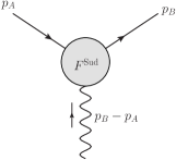
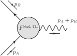
(a)	(b)

Figure 1: Graphs for the space-like (a) and time-like (b) quark form factor.

Let $F^{\text{Sud}}_{j}(Q_{E}^{2})$ be the quark form factor, defined in App. A, for the space-like electromagnetic process $\gamma^{*}(q)+q_{j}(p_{A})\to q_{j}(p_{B})$ on a quark of flavor $j$. It is illustrated in Fig. 1(a). The momentum transfer is $Q_{E}^{2}=-q^{2}=-(p_{B}-p_{A})^{2}$, normalized to be positive for a space-like virtual photon. The form-factor for the space-like process is purely real. It is normalized so that its lowest-order term is $1$. That is, a factor $e_{j}$ has been divided out, where $e_{j}$ is the charge of the quark.

Results for the Drell-Yan process are obtained from the form factor for the time-like process, $q_{j}(p_{A})+\bar{q}_{\bar{\jmath}}(p_{B})\to\gamma^{*}(q)$ [Fig. 1(b)]. The time-like form factor is obtained by analytic continuation of the space-like form factor to $Q_{E}^{2}=-Q^{2}-i\epsilon=-(p_{A}+p_{B})^{2}-i\epsilon$, to give $F^{\text{Sud, TL}}_{j\bar{\jmath}}(Q^{2})=F^{\text{Sud}}_{j}(-Q^{2}-i\epsilon)$.

VI.1 Factorization for form factor

Factorization for the form factor was treated in massless QCD in Magnea and Sterman (1990); Magnea (2001); Moch et al. (2005). We will use the specific formulation given by Collins in Ref. Collins (2011), with its definition of collinear factors in terms of an unsubtracted “collinear” matrix element and a combination of soft factors, with the relevant operators containing Wilson lines in particular directions. Collins (2011) gave results for the form factor in the case of a massive Abelian theory, but using methods later in Collins (2011), the results can be seen to generalize to massless QCD, with results generally compatible with those of Magnea and Sterman (1990); Magnea (2001); Moch et al. (2005). In this section, we will mostly use only the massless case, since that will be what is relevant for our calculations.

First we specify our conventions for how results are presented in terms of coupling dependence, and for our use of the $\overline{\rm MS}$ scheme. Renormalized quantities are written in terms of the coupling parameter $a_{s}$ defined in Eq. (1). The bare coupling, such as is used in the Lagrangian, has the form

$$a_{s,0}=\frac{\mu^{2\epsilon}}{S_{\epsilon}}a_{s}\left(1+\sum_{n=1}^{\infty}\sum_{m=1}^{n}A_{nm}\frac{a_{s}^{n}}{\epsilon^{m}}\right),$$ (27)

where the space-time dimension is $n=4-2\epsilon$, and

$$S_{\epsilon}=(4\pi e^{-\gamma_{\rm E}})^{\epsilon}.$$ (28)

The $\overline{\rm MS}$ scheme for coupling renormalization is defined by the requirement that the renormalization counterterms have the form shown in (27), where there is an overall factor $\mu^{2\epsilon}/S_{\epsilon}$, and there is otherwise a series of only negative powers of $\epsilon$ to make the counterterms. The conventions specified above for the $\overline{\rm MS}$ scheme correspond to those used by Moch et al. (2005).

The implementation of $\overline{\rm MS}$ in Ref. Collins (2011) differed in two ways. First there was a change of variable to replace $a_{s}$ by $a_{s}S_{\epsilon}$; this does not change the renormalized coupling at $\epsilon=0$ and so does not affect finite renormalized quantities at the physical space-time dimension. Second, the value of $S_{\epsilon}$ was changed to Collins (2011):

$$S^{\rm JCC}_{\epsilon}=\frac{(4\pi)^{\epsilon}}{\Gamma(1-\epsilon)}.$$ (29)

This has an advantage for the presentation of quantities whose counterterms have 2 poles per loop. The use of the form (29) for $S_{\epsilon}$ amounts to a change of scheme for such quantities. But it is currently less standard, so our main results will use the standard form.

For the calculations to be presented here, we will work within pure perturbation theory in strictly massless QCD. Then the power-suppressed corrections, such as we notated in earlier statements of TMD factorization, are zero. Factorization for the time-like form factor in massless QCD has the form

$$F^{\text{Sud}}_{j}\mathopen{}\left(\frac{-Q^{2}-i\epsilon}{\mu^{2}};a_{s}(\mu),\epsilon\right)\\ =H^{\text{Sud}}_{j}\mathopen{}\left(\frac{-Q^{2}-i\epsilon}{\mu^{2}};a_{s}(\mu),\epsilon\right)\left[C_{j}^{\rm Sud}(Q^{2},\mu,a_{s}(\mu),\epsilon)\right]^{2},$$ (30)

in the notation of App. A. Here $H^{\text{Sud}}_{j}$ is the hard factor, finite as $\epsilon\to 0$, with subtractions for all collinear and soft contributions. One of the collinear factors $C_{j}$ is for the quark of flavor $j$. Its first argument is the CSS $\zeta$ argument set to the value $Q^{2}$. The second collinear factor is for the antiquark, and by charge-conjugation invariance it equals the quark’s collinear factor. By use of the operator definitions given in (Collins, 2011, Ch. 10), the collinear factors include to leading power not only all contributions from collinear momenta but all soft contributions as well. To achieve this correctly, the Wilson lines used in the operator matrix elements used to define $C_{j}$ must be past pointing when the quark and antiquark are incoming Collins (2011).

We will also use factorization for the space-like case. By results in App. A, one of the collinear factors must be complex conjugated, so that we have:

$$F^{\text{Sud}}_{j}(Q_{E}^{2}/\mu^{2};a_{s}(\mu),\epsilon)\\ =H^{\text{Sud}}_{j}(Q_{E}^{2}/\mu^{2};a_{s}(\mu),\epsilon)\left|C^{\rm Sud}_{j}(Q_{E}^{2},\mu,a_{s}(\mu),\epsilon)\right|^{2},$$ (31)

with $Q_{E}^{2}$ being positive for the space-like case. Both of $F$ and $H$ are now real.

In each of Eqs. (30) and (31), the different factors on the right-hand side depend on the same variables, so at first sight there might appear to be no content. The significance of factorization is from the segregation of contributions from different regions of momenta. The lack of collinear and soft contributions to $H^{\rm Sud}$ imply that it has no divergences and also has no large logarithms when $\mu$ is of order $Q$; then it can be predicted perturbatively when $Q$ is large enough. The collinear factors have collinear and soft contributions, and they diverge in the massless limit. Furthermore, their definition allows useful equations to be derived for both their $\mu$ and $Q$ dependence. If masses were restored, then Eqs. (30) and (31) would be true to leading power in masses divided by $Q$ for large $Q$, and the collinear factors would be mass-dependent, but the hard factor would remain mass-independent with an unchanged value.

We will use evolution equations in the form found in Ref. Collins (2011). In addition, we will need extra results derived in App. A concerning the real and imaginary parts of the anomalous dimensions; these will be important in relating anomalous dimensions for the form factor to anomalous dimensions for the Drell-Yan process.

The renormalization-group (RG) equation for the collinear factor is

$$\frac{\mathop{\mathrm{d}\mskip-0.59999mu\ln C^{\rm Sud}_{j}}\nolimits}{\mathop{\mathrm{d}\mskip-0.59999mu\ln\mu}\nolimits}$$

$$={} \frac{1}{2}\gamma_{j}(a_{s}(\mu))+i\frac{\pi}{4}\gamma_{K}(a_{s}(\mu))-\frac{1}{4}\gamma_{K}(a_{s}(\mu))\ln\frac{Q^{2}}{\mu^{2}}$$

$$={} \frac{1}{2}\gamma_{j}(a_{s}(\mu))-\frac{1}{4}\gamma_{K}(a_{s}(\mu))\ln\frac{-Q^{2}-i\epsilon}{\mu^{2}}.$$ (32)

It is proved in App. A that the anomalous dimension functions $\gamma_{j}$ and $\gamma_{K}$ are both real, and that the imaginary part on the right-hand side is as shown. The normalizations of these functions are arranged so that they are exactly the same as the corresponding quantities in TMD factorization for the Drell-Yan process, with conventions as in Ref. Collins and Rogers (2015). The equality of these quantities between the Drell-Yan cross section and the Sudakov form factor is because the anomalous dimensions are determined by the renormalization of the same virtual loops containing the same operators. Their contribution to the Drell-Yan cross section is obtained by the absolute value squared of the sum of graphs for the form factor. Thus $H^{\text{DY}}_{j\bar{\jmath}}=|H^{\text{Sud}}_{j}((-Q^{2}-i\epsilon)/\mu^{2})|^{2}$, while the anomalous dimensions are $\gamma_{j}$ and $\gamma_{K}$, with cancellation of the imaginary part that appears in Eq. (VI.1).

Note that sometimes Collins (2011) $\gamma_{j}(a_{s}(\mu))$ is given a second argument, as in $\gamma_{j}(a_{s}(\mu);\zeta/\mu^{2})$. The $\zeta$ dependence corresponds to the $Q^{2}$ dependence in Eq. (VI.1), and $\gamma_{j}(a_{s}(\mu))$ in Eqs. (VI.1) and (35) corresponds to $\gamma_{j}(a_{s}(\mu);1)$ in the other notation.

The rapidity evolution equation for the collinear factor is

$$\frac{\partial C_{j}^{\rm Sud}}{\partial\ln Q}=\frac{1}{2}K^{\rm Sud}(a_{s},\epsilon),$$ (33)

with $K^{\rm Sud}$ obeying the RG equation

$$\frac{\mathop{\mathrm{d}\mskip-0.59999muK^{\rm Sud}}\nolimits}{\mathop{\mathrm{d}\mskip-0.59999mu\ln\mu}\nolimits}=-\gamma_{K}(a_{s})\,.$$ (34)

Note that $K^{\rm Sud}$ has no explicit dependence on $Q$ and $\mu$; it has soft divergences as $\epsilon\to 0$, and would be finite (but mass dependent) in a massive theory or in a theory with confinement.

In the remainder of this section, we will work with the time-like form factor and hard part, using the notations $F^{\text{Sud,~{}TL}}=F^{\text{Sud}}_{j}((-Q^{2}-i\epsilon)/\mu^{2})$ and $H^{\text{Sud,~{}TL}}=H^{\text{Sud}}_{j}((-Q^{2}-i\epsilon)/\mu^{2})$.

Since the form factor is RG-invariant, it follows from Eqs. (30) and (VI.1) that the RG equation for $H$ is

$$\frac{\mathop{\mathrm{d}\mskip-0.59999mu\ln H^{\text{Sud,~{}TL}}}\nolimits}{\mathop{\mathrm{d}\mskip-0.59999mu\ln\mu}\nolimits}\\ =-\gamma_{j}(a_{s}(\mu))-i\frac{\pi}{2}\gamma_{K}(a_{s}(\mu))+\frac{1}{2}\gamma_{K}(a_{s}(\mu))\ln\frac{Q^{2}}{\mu^{2}}.$$ (35)

Each of the collinear factors in factorization (30) is a bare collinear factor times an ultra-violet renormalization factor. It will be convenient to work with logarithms of the factors, for which renormalization is additive. We have

$$\ln F^{\rm Sud,~{}TL}(Q^{2})=\ln H^{\rm Sud,~{}TL}+2\ln C_{j}^{\rm bare}\\ +D(a_{s},\epsilon)-i\pi E(a_{s},\epsilon)+\ln\frac{Q^{2}}{\mu^{2}}E(a_{s},\epsilon)\,,$$ (36)

where the terms involving $E$ and $D$ implement counterterms for $\ln C_{j}$; the linearity in $\ln(Q^{2}/\mu^{2})$ follows from Eq. (33), and the lack of $Q$ dependence of $K^{\rm Sud}$. It is shown in App. A that each of $D$ and $E$ is real, and that there is an imaginary term $-i\pi E$, as in Eq. (36). Each of $D$ and $E$ has the usual $\overline{\rm MS}$ form:

$$D={} \sum_{n=1}^{\infty}\sum_{m=1}^{n+1}D_{nm}\frac{a_{s}^{n}}{\epsilon^{m}}$$ (37)

$$E={} \sum_{n=1}^{\infty}\sum_{m=1}^{n}E_{nm}\frac{a_{s}^{n}}{\epsilon^{m}}\,.$$ (38)

That the highest powers of $1/\epsilon$ in each order are as shown can be deduced from the evolution equations.

In the massless case, all loop integrals for the unsubtracted bare collinear factor are scale-free and hence zero Magnea and Sterman (1990); Magnea (2001). There remains only the lowest order term, which is unity. Hence, to all orders of perturbation theory $\ln C^{\rm bare}_{j}=0$. Therefore

$$\ln H^{\rm Sud,~{}TL}(Q^{2})=\\ \ln F^{\rm Sud,~{}TL}(Q^{2})-D+i\pi E-\ln\frac{Q^{2}}{\mu^{2}}E\quad\text{(massless),}$$ (39)

so that the finite quantity $\ln H^{\rm Sud}$ can be obtained from the massless $\ln F^{\rm Sud}$ simply by subtracting $\overline{\rm MS}$ poles. The poles initially arise as ultra-violet counterterms. But because of the zero value of the scale-free integrals for the collinear factor, these counterterms now subtract numerically opposite collinear and soft divergences in the logarithm of the form factor, $\ln F$.

We show in App. A that almost the same formula applies to the space-like case, with $F$ replaced by its space-like version, with omission of the imaginary term $i\pi E$ and with otherwise the same values of $D$ and $E$. It follows that the space-like hard part is obtained from the time-like hard part by the same analytic continuation that applies to the form factor itself. We have already used this result in discussing Eq. (31).

Now in RG equations for the massless theory, the derivative of any quantity $X$ with respect to $\mu$ is

$$\frac{\mathop{\mathrm{d}\mskip-0.59999muX}\nolimits}{\mathop{\mathrm{d}\mskip-0.59999mu\ln\mu}\nolimits}=\frac{\partial X}{\partial\ln\mu}-2\left(\epsilon a_{s}+\sum_{n=0}^{\infty}\beta_{n}a_{s}^{n+2}\right)\frac{\partial X}{\partial a_{s}},$$ (40)

where the $\beta_{n}$ are the usual coefficients that control the running of the coupling; they can obtained from the expansion of the bare coupling in powers of the renormalized coupling. In the calculations in this paper we will only need the following terms:

$$a_{s,0}=\frac{\mu^{2\epsilon}}{S_{\epsilon}}a_{s}\left[1-\beta_{0}\frac{a_{s}}{\epsilon}+a_{s}^{2}\left(\frac{\beta_{0}^{2}}{\epsilon^{2}}-\frac{\beta_{1}}{2\epsilon}\right)+\dots\right],$$ (41)

with the well-known values

$$\beta_{0}={} \frac{11}{3}C_{A}-\frac{2}{3}n_{f},$$ (42a)

$$\beta_{1}={} \frac{34}{3}C_{A}^{2}-\frac{10}{3}C_{A}n_{f}-2C_{F}n_{f}.$$ (42b)

The pole terms in the massless $\ln F^{\rm Sud,~{}TL}$ enable us to deduce $D$ and $E$ (from Eq. (39) given that $H^{\rm Sud}$ is finite), and hence the anomalous dimensions. The calculation of the anomalous dimensions arise because the renormalized collinear factor obeys

$$2\ln C^{\rm Sud}={} 2\ln C^{\rm bare}+D-i\pi E+\ln\frac{Q^{2}}{\mu^{2}}E,$$

$$={} D-i\pi E+\ln\frac{Q^{2}}{\mu^{2}}E\qquad\mbox{(massless)},$$ (43)

and the bare quantity is RG invariant. From (VI.1) we find

$$\gamma_{j}-\frac{1}{2}\ln\frac{Q^{2}}{\mu^{2}}\gamma_{K}=\frac{\mathop{\mathrm{d}\mskip-0.59999mu(D+\ln\frac{Q^{2}}{\mu^{2}}E)}\nolimits}{\mathop{\mathrm{d}\mskip-0.59999mu\ln\mu}\nolimits}=-2E-2\left(\epsilon a_{s}+\sum_{n=0}^{\infty}\beta_{n}a_{s}^{n+2}\right)\frac{\partial(D+\ln\frac{Q_{E}^{2}}{\mu^{2}}E)}{\partial a_{s}}\,,$$ (44)

Hence

$$\gamma_{K}=4\left(\epsilon a_{s}+\sum_{n=0}^{\infty}\beta_{n}a_{s}^{n+2}\right)\frac{\partial E}{\partial a_{s}}$$ (45)

and

$$\gamma_{j}=-2E-2\left(\epsilon a_{s}+\sum_{n=0}^{\infty}\beta_{n}a_{s}^{n+2}\right)\frac{\partial D}{\partial a_{s}}.$$ (46)

Let us define the expansions

$$\gamma_{K}={} \sum_{n=1}^{\infty}\gamma_{K,n}a_{s}^{n}\,,$$ (47)

$$\gamma_{j}={} \sum_{n=1}^{\infty}\gamma_{j,n}a_{s}^{n}\,.$$ (48)

Matching terms on each side of Eqs. (45) and (46), we deduce that the first two coefficients in $\gamma_{K}$ are obtained from the single-pole counterterms in $E$:

$$\gamma_{K,1}={} 4E_{1,1},$$ (49a)

$$\gamma_{K,2}={} 8E_{2,1}.$$ (49b)

The higher-pole counterterms are then determined since $\gamma_{K}$ has no $1/\epsilon$ poles. So all such poles must cancel on the right side of Eqs. (45) and (46). This gives

$$E_{2,2}=-\frac{\beta_{0}\gamma_{K,1}}{8}.$$ (50)

Similar equations apply at higher orders, but we do not derive them here.

Similarly, for $\gamma_{j}$ and $D$, we have

$$\gamma_{j,1}={} -2D_{1,1},$$ (51a)

$$\gamma_{j,2}={} -4D_{2,1},$$ (51b)

and

$$D_{1,2}={} -\frac{\gamma_{K,1}}{4},$$ (52a)

$$D_{2,3}={} \frac{3\beta_{0}\gamma_{K,1}}{16},$$ (52b)

$$D_{2,2}={} \frac{\beta_{0}\gamma_{j,1}}{4}-\frac{\gamma_{K,2}}{16}.$$ (52c)

VI.2 Coefficients for quark form factor

To obtain the actual values for the coefficients for the anomalous dimensions and the hard factor, we start from results for the massless form factor that were presented in Ref. Moch et al. (2005) as an expansion in powers of the bare coupling:

$$F^{\rm Sud}=1+\sum_{n=1}^{\infty}\left(a_{s,0}S_{\epsilon}Q_{E}^{-2\epsilon}\right)^{n}\mathcal{F}_{n}(\epsilon),$$ (53)

with $Q_{E}^{2}=-Q^{2}-i\epsilon$ for the time-like case that we need to obtain results for the Drell-Yan process. We then express the form factor in terms of the renormalized coupling by Eq. (27), of which we will only need the two-loop expansion (41).

We use Laurent expansions about $\epsilon=0$ of the coefficients $\mathcal{F}_{n}(\epsilon)$ in Eq. (53), with the notation

$$\mathcal{F}_{n}(\epsilon)=\sum_{m=-\infty}^{2n}\frac{F_{n,m}}{\epsilon^{m}}.$$ (54)

That the highest power of $1/\epsilon$ is twice the number of loops can be obtained from the evolution equations. For our calculations, values for the relevant coefficients $F_{n,m}$ can be read off Eqs. (3.5) and (3.6) in Moch et al. (2005).

The logarithm of the form factor has the following expansion in powers of the renormalized coupling

$$\ln F^{\rm Sud}=a_{s}\left(\frac{Q_{E}^{2}}{\mu^{2}}\right)^{-\epsilon}\mathcal{F}_{1}(\epsilon)+a_{s}^{2}\left(\frac{Q_{E}^{2}}{\mu^{2}}\right)^{-2\epsilon}\left[\mathcal{F}_{2}(\epsilon)-\frac{\mathcal{F}_{1}(\epsilon)^{2}}{2}\right]-a_{s}^{2}\left(\frac{Q_{E}^{2}}{\mu^{2}}\right)^{-\epsilon}\frac{\beta_{0}\mathcal{F}_{1}(\epsilon)}{\epsilon}+O(a_{s}^{3}).$$ (55)

Now Eq. (39) shows that we can determine $D$ and $E$ from the poles at $\epsilon=0$ in the coefficients in (55), and $\ln H$ from the finite remainder. For $D$ and $E$ we used a Mathematica program to obtain the following values up to 3-loop order from coefficients in Ref. Moch et al. (2005):

$$D={} -a_{s}C_{F}\left(\frac{2}{\epsilon^{2}}+\frac{3}{\epsilon}\right)$$

$$+a_{s}^{2}\Biggl{\{}C_{F}^{2}\left[\frac{-\frac{3}{4}+\pi^{2}-12\zeta_{3}}{\epsilon}\right]+C_{A}C_{F}\left[\frac{\frac{11}{2}}{\epsilon^{3}}+\frac{\frac{16}{9}+\frac{\pi^{2}}{6}}{\epsilon^{2}}+\frac{-\frac{961}{108}-\frac{11\pi^{2}}{12}+13\zeta_{3}}{\epsilon}\right]+n_{f}C_{F}\left[-\frac{1}{\epsilon^{3}}-\frac{\frac{4}{9}}{\epsilon^{2}}+\frac{\frac{65}{54}+\frac{\pi^{2}}{6}}{\epsilon}\right]\Biggr{\}}$$

$$+a_{s}^{3}\Biggl{\{}C_{F}n_{f}^{2}\left[-\frac{44}{81\epsilon^{4}}-\frac{8}{243\epsilon^{3}}+\frac{1}{\epsilon^{2}}\left(\frac{46}{81}+\frac{2\pi^{2}}{27}\right)+\frac{1}{\epsilon}\left(\frac{2417}{2187}-\frac{10\pi^{2}}{81}-\frac{8\zeta_{3}}{81}\right)\right]$$

$$\hskip 28.45274pt+C_{F}^{2}n_{f}\left[-\frac{16}{9\epsilon^{3}}+\frac{1}{\epsilon^{2}}\left(-\frac{8}{27}+\frac{4\pi^{2}}{9}-\frac{64\zeta_{3}}{9}\right)+\frac{1}{\epsilon}\left(\frac{2953}{162}-\frac{13\pi^{2}}{27}-\frac{14\pi^{4}}{81}+\frac{256\zeta_{3}}{27}\right)\right]$$

$$\hskip 28.45274pt+C_{A}^{2}C_{F}\left[-\frac{1331}{81\epsilon^{4}}+\frac{1}{\epsilon^{3}}\left(\frac{2866}{243}-\frac{55\pi^{2}}{81}\right)+\frac{1}{\epsilon^{2}}\left(\frac{11669}{486}+\frac{1625\pi^{2}}{486}-\frac{22\pi^{4}}{405}-\frac{902\zeta_{3}}{27}\right)\right.$$

$$\hskip 71.13188pt\left.+\frac{1}{\epsilon}\left(-\frac{139345}{8748}-\frac{7163\pi^{2}}{1458}-\frac{83\pi^{4}}{270}+\frac{3526\zeta_{3}}{27}-\frac{44\pi^{2}\zeta_{3}}{27}-\frac{136\zeta_{5}}{3}\right)\right]$$

$$\hskip 28.45274pt+\frac{C_{F}^{3}}{\epsilon}\left(-\frac{29}{6}-\pi^{2}-\frac{8\pi^{4}}{15}-\frac{68\zeta_{3}}{3}+\frac{16\pi^{2}\zeta_{3}}{9}+80\zeta_{5}\right)$$

$$\hskip 28.45274pt+C_{A}C_{F}n_{f}\left[\frac{484}{81\epsilon^{4}}+\frac{1}{\epsilon^{3}}\left(-\frac{752}{243}+\frac{10\pi^{2}}{81}\right)+\frac{1}{\epsilon^{2}}\left(-\frac{2068}{243}-\frac{238\pi^{2}}{243}+\frac{212\zeta_{3}}{27}\right)\right.$$

$$\hskip 85.35826pt\left.+\frac{1}{\epsilon}\left(-\frac{8659}{2187}+\frac{1297\pi^{2}}{729}+\frac{11\pi^{4}}{135}-\frac{964\zeta_{3}}{81}\right)\right]$$

$$\hskip 28.45274pt+C_{A}C_{F}^{2}\left[\frac{1}{\epsilon^{2}}\left(\frac{11}{6}-\frac{22\pi^{2}}{9}+\frac{88\zeta_{3}}{3\epsilon^{2}}\right)+\frac{1}{\epsilon}\left(-\frac{151}{12}+\frac{205\pi^{2}}{27}+\frac{247\pi^{4}}{405}-\frac{844\zeta_{3}}{9}-\frac{8\pi^{2}\zeta_{3}}{9}-40\zeta_{5}\right)\right]\Biggr{\}}$$

$$+O(a_{s}^{4}),$$ (56)

$$E={} a_{s}\frac{2C_{F}}{\epsilon}+a_{s}^{2}\Biggl{\{}C_{F}C_{A}\left[-\frac{11}{3\epsilon^{2}}+\frac{1}{\epsilon}\left(\frac{67}{9}-\frac{\pi^{2}}{3}\right)\right]+C_{F}n_{f}\left[\frac{2}{3\epsilon^{2}}-\frac{10}{9\epsilon}\right]\Biggr{\}}$$

$$+a_{s}^{3}\Biggl{\{}C_{F}n_{f}^{2}\left[\frac{8}{27\epsilon^{3}}-\frac{40}{81\epsilon^{2}}-\frac{8}{81\epsilon}\right]+C_{A}C_{F}n_{f}\left[-\frac{88}{27\epsilon^{3}}+\frac{1}{\epsilon^{2}}\left(\frac{668}{81}-\frac{4\pi^{2}}{27}\right)+\frac{1}{\epsilon}\left(-\frac{418}{81}+\frac{40\pi^{2}}{81}-\frac{56\zeta_{3}}{9}\right)\right]$$

$$\hskip 28.45274pt+C_{A}^{2}C_{F}\left[\frac{242}{27\epsilon^{3}}+\frac{1}{\epsilon^{2}}\left(-\frac{2086}{81}+\frac{22\pi^{2}}{27}\right)+\frac{1}{\epsilon}\left(\frac{245}{9}-\frac{268\pi^{2}}{81}+\frac{22\pi^{4}}{135}+\frac{44\zeta_{3}}{9}\right)\right]$$

$$\hskip 28.45274pt+C_{F}^{2}n_{f}\left[\frac{4}{3\epsilon^{2}}+\frac{1}{\epsilon}\left(-\frac{55}{9}+\frac{16\zeta_{3}}{3}\right)\right]\Biggr{\}}$$

$$+O(a_{s}^{4}).$$ (57)

The values for $\gamma_{j}$ and $\gamma_{K}$ are deduced from Eqs. (45) and (46):

$$\gamma_{j}={} 6C_{F}a_{s}+a_{s}^{2}\left[C_{F}^{2}\left(3-4\pi^{2}+48\zeta_{3}\right)+C_{F}C_{A}\left(\frac{961}{27}+\frac{11\pi^{2}}{3}-52\zeta_{3}\right)+C_{F}n_{f}\left(-\frac{130}{27}-\frac{2\pi^{2}}{3}\right)\right]$$

$$+a_{s}^{3}\biggl{[}C_{F}^{2}n_{f}\left(-\frac{2953}{27}+\frac{26\pi^{2}}{9}+\frac{28\pi^{4}}{27}-\frac{512\zeta_{3}}{9}\right)+C_{F}n_{f}^{2}\left(-\frac{4834}{729}+\frac{20\pi^{2}}{27}+\frac{16\zeta_{3}}{27}\right)$$

$$\hskip 28.45274pt+C_{F}^{3}\left(29+6\pi^{2}+\frac{16\pi^{4}}{5}+136\zeta_{3}-\frac{32\pi^{2}\zeta_{3}}{3}-480\zeta_{5}\right)$$

$$\hskip 28.45274pt+C_{A}^{2}C_{F}\left(\frac{139345}{1458}+\frac{7163\pi^{2}}{243}+\frac{83\pi^{4}}{45}-\frac{7052\zeta_{3}}{9}+\frac{88\pi^{2}\zeta_{3}}{9}+272\zeta_{5}\right)$$

$$\hskip 28.45274pt+C_{A}C_{F}n_{f}\left(\frac{17318}{729}-\frac{2594\pi^{2}}{243}-\frac{22\pi^{4}}{45}+\frac{1928\zeta_{3}}{27}\right)$$

$$\hskip 28.45274pt+C_{A}C_{F}^{2}\left(\frac{151}{2}-\frac{410\pi^{2}}{9}-\frac{494\pi^{4}}{135}+\frac{1688\zeta_{3}}{3}+\frac{16\pi^{2}\zeta_{3}}{3}+240\zeta_{5}\right)\biggr{]}$$

$$+O(a_{s}^{4}),$$ (58)

$$\gamma_{K}={} 8C_{F}a_{s}+a_{s}^{2}\left[C_{A}C_{F}\left(\frac{536}{9}-\frac{8\pi^{2}}{3}\right)-\frac{80}{9}C_{F}n_{f}\right]$$

$$+a_{s}^{3}\left[-\frac{32}{27}C_{F}n_{f}^{2}+C_{A}C_{F}n_{f}\left(-\frac{1672}{27}+\frac{160\pi^{2}}{27}-\frac{224\zeta_{3}}{3}\right)+C_{A}^{2}C_{F}\left(\frac{980}{3}-\frac{1072\pi^{2}}{27}+\frac{88\pi^{4}}{45}+\frac{176\zeta_{3}}{3}\right)\right.$$

$$\hskip 28.45274pt\left.+C_{F}^{2}n_{f}\left(-\frac{220}{3}+64\zeta_{3}\right)\right]$$

$$+O(a_{s}^{4}).$$ (59)

We also verify that the consistency conditions (50) and (52) are obeyed. The above values are in agreement with the results of Gehrmann et al. (2010), after allowing for the different normalizations of their anomalous dimensions.

Finally, the Sudakov hard factor at $\epsilon=0$ is

$$H^{\text{Sud}}={} 1+C_{F}a_{s}\left(-8+\frac{\pi^{2}}{6}+3t-t^{2}\right)$$

$$+a_{s}^{2}\Biggl{\{}C_{F}^{2}\left[\frac{255}{8}+\frac{7\pi^{2}}{2}-\frac{83\pi^{4}}{360}-30\zeta_{3}+t\left(-\frac{45}{2}-\frac{3\pi^{2}}{2}+24\zeta_{3}\right)+t^{2}\left(\frac{25}{2}-\frac{\pi^{2}}{6}\right)-3t^{3}+\frac{1}{2}t^{4}\right]$$

$$+C_{F}C_{A}\Biggl{[}-\frac{51157}{648}-\frac{337\pi^{2}}{108}+\frac{11\pi^{4}}{45}+\frac{313}{9}\zeta_{3}+t\left(\frac{2545}{54}+\frac{11\pi^{2}}{9}-26\zeta_{3}\right)+t^{2}\left(-\frac{233}{18}+\frac{\pi^{2}}{3}\right)+\frac{11}{9}t^{3}\Biggr{]}$$

$$+C_{F}n_{f}\Biggl{[}\frac{4085}{324}+\frac{23\pi^{2}}{54}+\frac{2}{9}\zeta_{3}+t\left(-\frac{209}{27}-\frac{2\pi^{2}}{9}\right)+\frac{19}{9}t^{2}-\frac{2}{9}t^{3}\Biggr{]}\Biggr{\}}$$

$${}+a_{s}^{3}\Biggl{\{}C_{F}^{3}\Biggl{[}16\zeta_{3}^{2}+\frac{125\pi^{2}\zeta_{3}}{3}-470\zeta_{3}+664\zeta_{5}+\frac{37729\pi^{6}}{136080}-\frac{413\pi^{4}}{180}-\frac{6451\pi^{2}}{144}-\frac{2539}{12}$$

$$\hskip 19.91692pt+t\left(-\frac{4}{3}\pi^{2}\zeta_{3}-214\zeta_{3}-240\zeta_{5}+\frac{23\pi^{4}}{40}+\frac{119\pi^{2}}{4}+\frac{785}{8}\right)+t^{2}\left(102\zeta_{3}+\frac{83\pi^{4}}{360}-\frac{35\pi^{2}}{4}-\frac{507}{8}\right)$$

$$\hskip 19.91692pt+t^{3}\left(-24\zeta_{3}+\frac{3\pi^{2}}{2}+27\right)+t^{4}\left(\frac{\pi^{2}}{12}-\frac{17}{2}\right)+\frac{3t^{5}}{2}-\frac{t^{6}}{6}\Biggr{]}$$

$$+C_{F}^{2}n_{f}\Biggl{[}\frac{41077}{972}-\frac{416}{9}\zeta_{5}+\frac{13184}{81}\zeta_{3}-\frac{31729\pi^{2}}{1944}-\frac{19\pi^{2}}{27}\zeta_{3}-\frac{331\pi^{4}}{972}$$

$$\hskip 36.98857pt+t\bigg{(}\frac{3121}{108}-\frac{610}{9}\zeta_{3}+\frac{809\pi^{2}}{81}+\frac{7\pi^{4}}{45}\bigg{)}$$

$$\hskip 36.98857pt+t^{2}\bigg{(}-\frac{12815}{324}+\frac{70}{9}\zeta_{3}-\frac{56\pi^{2}}{27}\bigg{)}+t^{3}\bigg{(}\frac{410}{27}+\frac{5\pi^{2}}{27}\bigg{)}-\frac{25}{9}t^{4}+\frac{2}{9}t^{5}\Biggr{]}$$

$$+C_{A}C_{F}^{2}\Biggl{[}\frac{296\zeta_{3}^{2}}{3}-\frac{3751\pi^{2}\zeta_{3}}{54}-\frac{18770\zeta_{3}}{27}-\frac{2756\zeta_{5}}{9}-\frac{3169\pi^{6}}{17010}-\frac{4943\pi^{4}}{9720}+\frac{538835\pi^{2}}{3888}+\frac{415025}{648}$$

$$\hskip 42.67912pt+t\left(-\frac{5}{3}\pi^{2}\zeta_{3}+\frac{2441\zeta_{3}}{3}+120\zeta_{5}+\frac{9\pi^{4}}{10}-\frac{5630\pi^{2}}{81}-\frac{13805}{24}\right)$$

$$\hskip 42.67912pt+t^{2}\left(-\frac{1807\zeta_{3}}{9}-\frac{17\pi^{4}}{90}+\frac{251\pi^{2}}{27}+\frac{206317}{648}\right)+t^{3}\left(26\zeta_{3}-\frac{\pi^{2}}{54}-\frac{2585}{27}\right)+t^{4}\left(\frac{299}{18}-\frac{\pi^{2}}{3}\right)-\frac{11t^{5}}{9}\Biggr{]}$$

$$+C_{A}^{2}C_{F}\Biggl{[}-\frac{1136\zeta_{3}^{2}}{9}+\frac{208\pi^{2}\zeta_{3}}{9}+\frac{505087\zeta_{3}}{486}-\frac{434\zeta_{5}}{9}-\frac{769\pi^{6}}{5103}+\frac{22157\pi^{4}}{9720}-\frac{412315\pi^{2}}{4374}-\frac{51082685}{52488}$$

$$\hskip 42.67912pt+t\left(\frac{44\pi^{2}\zeta_{3}}{9}-\frac{17464\zeta_{3}}{27}+136\zeta_{5}-\frac{47\pi^{4}}{54}+\frac{8683\pi^{2}}{243}+\frac{1045955}{1458}\right)$$

$$\hskip 42.67912pt+t^{2}\left(88\zeta_{3}-\frac{11\pi^{4}}{45}+\frac{13\pi^{2}}{27}-\frac{18682}{81}\right)+t^{3}\left(\frac{2869}{81}-\frac{22\pi^{2}}{27}\right)-\frac{121t^{4}}{54}\Biggr{]}$$

$$+C_{A}C_{F}n_{f}\Biggl{[}\frac{2\pi^{2}\zeta_{3}}{9}-\frac{4288\zeta_{3}}{27}-\frac{4\zeta_{5}}{3}+\frac{\pi^{4}}{486}+\frac{115555\pi^{2}}{4374}+\frac{1700171}{6561}$$

$$\hskip 54.06023pt+\left(\frac{724\zeta_{3}}{9}+\frac{11\pi^{4}}{135}-\frac{2932\pi^{2}}{243}-\frac{154919}{729}\right)t$$

$$\hskip 54.06023pt+\left(-8\zeta_{3}+\frac{8\pi^{2}}{9}+\frac{5876}{81}\right)t^{2}+\left(\frac{4\pi^{2}}{27}-\frac{974}{81}\right)t^{3}+\frac{22t^{4}}{27}\Biggr{]}$$

$$+C_{F}n_{f}^{2}\Biggl{[}-\frac{416\zeta_{3}}{243}-\frac{47\pi^{4}}{1215}-\frac{412\pi^{2}}{243}-\frac{190931}{13122}+t\left(\frac{16\zeta_{3}}{27}+\frac{76\pi^{2}}{81}+\frac{9838}{729}\right)+t^{2}\left(-\frac{406}{81}-\frac{4\pi^{2}}{27}\right)$$

$$\hskip 56.9055pt+\frac{76t^{3}}{81}-\frac{2t^{4}}{27}\Biggr{]}$$

$$+\frac{C_{F}\left(N^{2}-4\right)N_{j,v}}{N}\Biggl{[}\frac{14\zeta_{3}}{3}-\frac{80\zeta_{5}}{3}-\frac{\pi^{4}}{90}+\frac{5\pi^{2}}{3}+4\Biggr{]}\Biggr{\}}\qquad+O(a_{s}^{4}),$$ (60)

where $t=\ln(Q_{E}^{2}/\mu^{2})=\ln((-Q^{2}-i\epsilon)/\mu^{2})=\ln(Q^{2}/\mu^{2})-i\pi$. The quantity $N_{j,v}$ is defined as

$$N_{j,v}\equiv\frac{\sum_{q}e_{q}}{e_{j}}\,.$$ (61)

and is needed for graphs first encountered at $a_{s}^{3}$ where the quark line at the electromagnetic current is in an internal loop instead of being connected to the external lines. Our own calculations are for the coefficient to order $a_{s}^{2}$, and are in agreement with the results first obtained from the same starting point by Idilbi et al. (2006). Unlike $\gamma_{K}$ and $\gamma_{j}$, we cannot extract the result for $H^{\text{Sud}}$ at order $a_{s}^{3}$ using the calculations in Ref. Moch et al. (2005) because the three-loop form factor given there includes the pole terms but not the constant term as a function of $\epsilon$. To get the order $a_{s}^{3}$ contribution, the above steps may be straightforwardly repeated using the full three-loop result in Eq. (5.4) of Ref. Gehrmann et al. (2010). Their results for $H^{\text{Sud}}$ are given in their Eqs. (7.4), (7.5), and (7.8). To make our Eq. (VI.2) a complete reference for the current state of knowledge, we have copied their order $a_{s}^{3}$ term.

In their paper reporting the form-factor calculations that we use, Moch et al. (2005) also obtain the anomalous dimension, for the quantity they call $A$, which equals $\gamma_{K}/2$. Although they use the same notation $A$ as in the CSS1 formulation, they have not performed the CSS1 redefinition of the factors, and so their $A$ matches our $\gamma_{K}$. There appears to be no quantity calculated in Moch et al. (2005) that corresponds directly to $\gamma_{j}$.

VII RG evolution of TMD parton densities and TMD fragmentation functions

The RG evolution of the TMD parton densities and TMD fragmentation functions is determined by their ultra-violet renormalization factors. In turn, the renormalization factors are determined completely from the virtual graphs at the vertices for the operators defining the TMD functions. These are exactly the same graphs as for the square of the absolute value of any collinear factor in the form factor case. Therefore, the renormalization factor for a TMD function is the same as the square of the absolute value of the renormalization factor of the corresponding collinear factor for the form factor. By the results of App. A.4, this square has the same value independently of whether the Wilson lines are future- or past-pointing and of whether the quark is initial-state or final- state. Thus the anomalous dimensions for the TMD functions are the same for TMD fragmentation functions and TMD parton densities, and they are also the same for the unpolarized TMD parton densities for SIDIS, with their past-pointing Wilson lines, and for the TMD parton densities for DY, with their future-pointing Wilson lines.

Hence in the RG equation (9) obeyed by the TMD parton densities, the anomalous dimensions $\gamma_{j}$ and $\gamma_{K}$ are the same as in the RG equation (VI.1) for the collinear factors for the quark form factor. Similarly the same anomalous dimensions are used in the RG equation for all the TMD fragmentation functions.

These relations have been known for some time from low-order calculations, but the present paper is the first place we know of where they are explicitly shown to be true generally. It is an especially important result because it means the complete evolution factor on the next-to-last line of Eq. (II.3) is strongly universal.

Note that these results do not imply equality for the coefficients $C^{\rm PDF}$ and $C^{\rm FF}$ that relate TMD functions and the corresponding collinear functions; superscripts “PDF” and “FF” should be kept there.

VIII Values of Drell-Yan and SIDIS quantities

In this section, we show in detail how to obtain values of the coefficients at order $a_{s}^{2}$ for the Drell-Yan process starting from results for collinear factorization and for the quark form factor.

VIII.1 Hard factor

Since the graphs and subtractions are the same, the hard factor for Drell-Yan scattering is obtained from the square of the hard factor for the time-like factor:

$$H_{j\bar{\jmath}}^{\rm DY}(Q,\mu;a_{s}(\mu))=e_{j}^{2}\left|H_{j}^{\text{Sud, TL}}(Q^{2})\right|^{2}=e_{j}^{2}\left|H_{j}^{\text{Sud}}(-Q^{2}-i\epsilon)\right|^{2}\,.$$ (62)

From Eq. (VI.2) we find

$$\frac{1}{e_{j}^{2}}H_{j\bar{\jmath}}^{\rm DY}(Q,\mu;a_{s}(\mu))={} 1+C_{F}a_{s}\left(-16+\frac{7\pi^{2}}{3}+6T-2T^{2}\right)$$

$$+a_{s}^{2}\Biggl{\{}C_{F}^{2}\left[\frac{511}{4}-\frac{83\pi^{2}}{3}+\frac{67\pi^{4}}{30}-60\zeta_{3}+T\left(-93+10\pi^{2}+48\zeta_{3}\right)+T^{2}\left(-\frac{14\pi^{2}}{3}+50\right)-12T^{3}+2T^{4}\right]$$

$$+C_{F}C_{A}\left[-\frac{51157}{324}+\frac{1061\pi^{2}}{54}-\frac{8\pi^{4}}{45}+\frac{626}{9}\zeta_{3}+T\left(\frac{2545}{27}-\frac{44\pi^{2}}{6}-52\zeta_{3}\right)+T^{2}\left(\frac{2\pi^{2}}{3}-\frac{233}{9}\right)+\frac{22}{9}T^{3}\right]$$

$$+n_{f}C_{F}\left[\frac{4085}{162}-\frac{91\pi^{2}}{27}+\frac{4}{9}\zeta_{3}+T\left(\frac{8\pi^{2}}{9}-\frac{418}{27}\right)+\frac{38}{9}T^{2}-\frac{4}{9}T^{3}\right]\Biggr{\}}$$

$$+a_{s}^{3}\Biggl{\{}C_{F}^{3}\Biggl{[}32\zeta_{3}^{2}-\frac{140\pi^{2}\zeta_{3}}{3}-460\zeta_{3}+1328\zeta_{5}+\frac{27403\pi^{6}}{17010}-\frac{346\pi^{4}}{15}+\frac{4339\pi^{2}}{36}-\frac{5599}{6}$$

$$+T\left(\frac{304\pi^{2}\zeta_{3}}{3}-992\zeta_{3}-480\zeta_{5}+\frac{109\pi^{4}}{15}-89\pi^{2}+\frac{1495}{2}\right)+T^{2}\left(408\zeta_{3}-\frac{67\pi^{4}}{15}+\frac{220\pi^{2}}{3}-\frac{1051}{2}\right)$$

$$+T^{3}\left(-96\zeta_{3}-20\pi^{2}+222\right)+T^{4}\left(\frac{14\pi^{2}}{3}-68\right)+12T^{5}-\frac{4T^{6}}{3}\Biggr{]}$$

$$+C_{A}C_{F}^{2}\Biggl{[}\frac{592\zeta_{3}^{2}}{3}+\frac{1690\pi^{2}\zeta_{3}}{9}-\frac{52564\zeta_{3}}{27}-\frac{5512\zeta_{5}}{9}-\frac{1478\pi^{6}}{1701}+\frac{92237\pi^{4}}{2430}-\frac{406507\pi^{2}}{972}+\frac{824281}{324}$$

$$+T\left(-116\pi^{2}\zeta_{3}+2252\zeta_{3}+240\zeta_{5}-\frac{1694\pi^{4}}{135}+\frac{24268\pi^{2}}{81}-\frac{14269}{6}\right)$$

$$+T^{2}\left(-\frac{5644\zeta_{3}}{9}+\frac{86\pi^{4}}{45}-\frac{3376\pi^{2}}{27}+\frac{208099}{162}\right)$$

$$+T^{3}\left(104\zeta_{3}+\frac{526\pi^{2}}{27}-\frac{10340}{27}\right)+T^{4}\left(\frac{598}{9}-\frac{4\pi^{2}}{3}\right)-\frac{44T^{5}}{9}\Biggr{]}$$

$$+C_{A}^{2}C_{F}\Biggl{[}-\frac{2272\zeta_{3}^{2}}{9}-\frac{1168\pi^{2}\zeta_{3}}{9}+\frac{505087\zeta_{3}}{243}-\frac{868\zeta_{5}}{9}+\frac{4784\pi^{6}}{25515}-\frac{4303\pi^{4}}{4860}+\frac{596513\pi^{2}}{2187}-\frac{51082685}{26244}$$

$$+T\left(\frac{88\pi^{2}\zeta_{3}}{9}-\frac{34928\zeta_{3}}{27}+272\zeta_{5}+\frac{85\pi^{4}}{27}-\frac{34276\pi^{2}}{243}+\frac{1045955}{729}\right)$$

$$+T^{2}\left(176\zeta_{3}-\frac{22\pi^{4}}{45}+\frac{752\pi^{2}}{27}-\frac{37364}{81}\right)+T^{3}\left(\frac{5738}{81}-\frac{44\pi^{2}}{27}\right)-\frac{121T^{4}}{27}\Biggr{]}$$

$$C_{A}C_{F}n_{f}\Biggl{[}\frac{148\pi^{2}\zeta_{3}}{9}-\frac{8576\zeta_{3}}{27}-\frac{8\zeta_{5}}{3}-\frac{35\pi^{4}}{243}-\frac{201749\pi^{2}}{2187}+\frac{3400342}{6561}$$

$$+T\left(\frac{1448\zeta_{3}}{9}-\frac{98\pi^{4}}{135}+\frac{11668\pi^{2}}{243}-\frac{309838}{729}\right)$$

$$+T^{2}\left(-16\zeta_{3}-8\pi^{2}+\frac{11752}{81}\right)+T^{3}\left(\frac{8\pi^{2}}{27}-\frac{1948}{81}\right)+\frac{44T^{4}}{27}\Biggr{]}$$

$$+C_{F}n_{f}^{2}\Biggl{[}-\frac{832\zeta_{3}}{243}+\frac{86\pi^{4}}{1215}+\frac{1612\pi^{2}}{243}-\frac{190931}{6561}+T\left(\frac{32\zeta_{3}}{27}-\frac{304\pi^{2}}{81}+\frac{19676}{729}\right)$$

$$+T^{2}\left(\frac{16\pi^{2}}{27}-\frac{812}{81}\right)+\frac{152T^{3}}{81}-\frac{4T^{4}}{27}\Biggr{]}$$

$$+C_{F}^{2}n_{f}\Biggl{[}-\frac{148}{9}\pi^{2}\zeta_{3}+\frac{26080\zeta_{3}}{81}-\frac{832\zeta_{5}}{9}-\frac{1463\pi^{4}}{243}+\frac{13705\pi^{2}}{243}-\frac{56963}{486}$$

$$+T\left(-\frac{1208\zeta_{3}}{9}+\frac{332\pi^{4}}{135}-\frac{4060\pi^{2}}{81}+\frac{6947}{27}\right)+T^{2}\left(\frac{136\zeta_{3}}{9}+\frac{520\pi^{2}}{27}-\frac{14948}{81}\right)$$

$$+T^{3}\left(\frac{1676}{27}-\frac{76\pi^{2}}{27}\right)-\frac{100T^{4}}{9}+\frac{8T^{5}}{9}\Biggr{]}$$

$$+C_{F}N_{j,v}\Biggl{[}\frac{28\zeta_{3}N}{3}-\frac{160\zeta_{5}N}{3}-\frac{112\zeta_{3}}{3N}+\frac{640\zeta_{5}}{3N}-\frac{\pi^{4}N}{45}+\frac{10\pi^{2}N}{3}+8N+\frac{4\pi^{4}}{45N}-\frac{40\pi^{2}}{3N}-\frac{32}{N}\Biggr{]}\Biggr{\}}~{}+O(a_{s}^{4})\,.$$ (63)

For SIDIS, we get

$$\frac{1}{e_{j}^{2}}H_{j\bar{\jmath}}^{\rm SIDIS}(Q,\mu;a_{s}(\mu))={} 1+C_{F}a_{s}\left(-16+\frac{\pi^{2}}{3}+6T-2T^{2}\right)$$

$$+a_{s}^{2}\Biggl{\{}C_{F}^{2}\left[\frac{511}{4}+\frac{13\pi^{2}}{3}-\frac{13\pi^{4}}{30}-60\zeta_{3}+T(-93-2\pi^{2}+48\zeta_{3})+T^{2}\Biggl{(}-\frac{2\pi^{2}}{3}+50\Biggr{)}-12T^{3}+2T^{4}\right]+$$

$$+C_{A}C_{F}\left[-\frac{51157}{324}-\frac{337\pi^{2}}{54}+\frac{22\pi^{4}}{45}+\frac{626\zeta_{3}}{9}+T\Biggl{(}\frac{2545}{27}+\frac{22\pi^{2}}{9}-52\zeta_{3}\Biggr{)}+T^{2}\left(\frac{2\pi^{2}}{3}-\frac{233}{9}\right)+\frac{22T^{3}}{9}\right]$$

$$+C_{F}n_{f}\left[\frac{4085}{162}+\frac{23\pi^{2}}{27}+\frac{4\zeta_{3}}{9}-T\left(\frac{418}{27}+\frac{4\pi^{2}}{9}\right)+\frac{38T^{2}}{9}-\frac{4T^{3}}{9}\right]\Biggr{\}}$$

$$+a_{s}^{3}\Biggl{\{}C_{F}^{3}\Biggl{[}32\zeta_{3}^{2}+\frac{220\pi^{2}\zeta_{3}}{3}-460\zeta_{3}+1328\zeta_{5}+\frac{1625\pi^{6}}{3402}+\frac{4\pi^{4}}{15}-\frac{4859\pi^{2}}{36}-\frac{5599}{6}$$

$$+T\left(\frac{16\pi^{2}\zeta_{3}}{3}-992\zeta_{3}-480\zeta_{5}-\frac{11\pi^{4}}{15}+97\pi^{2}+\frac{1495}{2}\right)+T^{2}\left(408\zeta_{3}+\frac{13\pi^{4}}{15}-\frac{80\pi^{2}}{3}-\frac{1051}{2}\right)$$

$$+T^{3}\left(-96\zeta_{3}+4\pi^{2}+222\right)+T^{4}\left(\frac{2\pi^{2}}{3}-68\right)+12T^{5}-\frac{4T^{6}}{3}\Biggr{]}$$

$$+C_{A}C_{F}^{2}\Biggl{[}\frac{592\zeta_{3}^{2}}{3}-\frac{382\pi^{2}\zeta_{3}}{3}-\frac{52564\zeta_{3}}{27}-\frac{5512\zeta_{5}}{9}-\frac{2476\pi^{6}}{8505}-\frac{14503\pi^{4}}{2430}+\frac{292367\pi^{2}}{972}+\frac{824281}{324}$$

$$+T\left(-12\pi^{2}\zeta_{3}+2252\zeta_{3}+240\zeta_{5}+\frac{496\pi^{4}}{135}-\frac{13088\pi^{2}}{81}-\frac{14269}{6}\right)$$

$$+T^{2}\left(-\frac{5644\zeta_{3}}{9}-\frac{34\pi^{4}}{45}+\frac{608\pi^{2}}{27}+\frac{208099}{162}\right)+T^{3}\left(104\zeta_{3}-\frac{2\pi^{2}}{27}-\frac{10340}{27}\right)$$

$$+T^{4}\left(\frac{598}{9}-\frac{4\pi^{2}}{3}\right)-\frac{44T^{5}}{9}\Biggr{]}$$

$$+C_{A}^{2}C_{F}\Biggl{[}-\frac{2272\zeta_{3}^{2}}{9}+\frac{416\pi^{2}\zeta_{3}}{9}+\frac{505087\zeta_{3}}{243}-\frac{868\zeta_{5}}{9}-\frac{1538\pi^{6}}{5103}+\frac{22157\pi^{4}}{4860}-\frac{412315\pi^{2}}{2187}-\frac{51082685}{26244}$$

$$+T\left(\frac{88\pi^{2}\zeta_{3}}{9}-\frac{34928\zeta_{3}}{27}+272\zeta_{5}-\frac{47\pi^{4}}{27}+\frac{17366\pi^{2}}{243}+\frac{1045955}{729}\right)$$

$$+T^{2}\left(176\zeta_{3}-\frac{22\pi^{4}}{45}+\frac{26\pi^{2}}{27}-\frac{37364}{81}\right)+T^{3}\left(\frac{5738}{81}-\frac{44\pi^{2}}{27}\right)-\frac{121T^{4}}{27}\Biggr{]}$$

$$C_{A}C_{F}n_{f}\Biggl{[}\frac{4\pi^{2}\zeta_{3}}{9}-\frac{8576\zeta_{3}}{27}-\frac{8\zeta_{5}}{3}+\frac{\pi^{4}}{243}+\frac{115555\pi^{2}}{2187}+\frac{3400342}{6561}$$

$$+T\left(\frac{1448\zeta_{3}}{9}+\frac{22\pi^{4}}{135}-\frac{5864\pi^{2}}{243}-\frac{309838}{729}\right)+T^{2}\left(-16\zeta_{3}+\frac{16\pi^{2}}{9}+\frac{11752}{81}\right)$$

$$+T^{3}\left(\frac{8\pi^{2}}{27}-\frac{1948}{81}\right)+\frac{44T^{4}}{27}\Biggr{]}$$

$$+C_{F}n_{f}^{2}\Biggl{[}-\frac{832\zeta_{3}}{243}-\frac{94\pi^{4}}{1215}-\frac{824\pi^{2}}{243}-\frac{190931}{6561}+T\left(\frac{32\zeta_{3}}{27}+\frac{152\pi^{2}}{81}+\frac{19676}{729}\right)$$

$$+T^{2}\left(-\frac{812}{81}-\frac{8\pi^{2}}{27}\right)+\frac{152T^{3}}{81}-\frac{4T^{4}}{27}\Biggr{]}$$

$$+C_{F}^{2}n_{f}\Biggl{[}-\frac{4}{3}\pi^{2}\zeta_{3}+\frac{26080\zeta_{3}}{81}-\frac{832\zeta_{5}}{9}-\frac{131\pi^{4}}{243}-\frac{8567\pi^{2}}{243}-\frac{56963}{486}$$

$$+T\left(-\frac{1208\zeta_{3}}{9}+\frac{32\pi^{4}}{135}+\frac{1904\pi^{2}}{81}+\frac{6947}{27}\right)$$

$$+T^{2}\left(\frac{136\zeta_{3}}{9}-\frac{152\pi^{2}}{27}-\frac{14948}{81}\right)+T^{3}\left(\frac{1676}{27}+\frac{20\pi^{2}}{27}\right)-\frac{100T^{4}}{9}+\frac{8T^{5}}{9}\Biggr{]}$$

$$+C_{F}N_{j,v}\Biggl{[}\frac{28\zeta_{3}N}{3}-\frac{160\zeta_{5}N}{3}-\frac{112\zeta_{3}}{3N}+\frac{640\zeta_{5}}{3N}-\frac{\pi^{4}N}{45}+\frac{10\pi^{2}N}{3}+8N+\frac{4\pi^{4}}{45N}-\frac{40\pi^{2}}{3N}-\frac{32}{N}\Biggr{]}\Biggr{\}}+O(a_{s}^{4})\,.$$ (64)

In both of these equations, $T=\ln(Q^{2}/\mu^{2})$, and $N_{j,v}$ is defined by Eq. (61). With $n_{f}=3$, the ratio of the Drell-Yan to SIDIS hard factors is

$$\frac{H_{j\bar{\jmath}}^{\rm DY}}{H_{j\bar{\jmath}}^{\rm SIDIS}}=1+2.0944\,\alpha_{s}(\mu)+5.96498\,\alpha_{s}(\mu)^{2}+18.6104\,\alpha_{s}(\mu)^{3}+O(\alpha_{s}^{4})\,,$$ (65)

and we have verified that we match Eq. (4.4) of Ref. Moch et al. (2005) for $n_{f}=4$.

In our later calculations, we will need the coefficients of the Drell-Yan hard factor at $T=0$, i.e., with $\mu=Q$ or $C_{2}=1$. So we write

$$\frac{1}{e_{j}^{2}}H_{j\bar{\jmath}}^{\rm DY}(Q,Q;a_{s}(Q))=1+\sum_{n=1}^{\infty}a_{s}^{n}\hat{H}_{j\bar{\jmath}}^{\text{DY }(n)},$$ (66)

and we have

$$\hat{H}_{j\bar{\jmath}}^{\text{DY }(1)}={} C_{F}\left(-16+\frac{7\pi^{2}}{3}\right),$$ (67a)

$$\hat{H}_{j\bar{\jmath}}^{\text{DY }(2)}={} C_{F}^{2}\left[\frac{511}{4}-\frac{83\pi^{2}}{3}+\frac{67\pi^{4}}{30}-60\zeta_{3}\right]+C_{F}C_{A}\left[-\frac{51157}{324}+\frac{1061\pi^{2}}{54}-\frac{8\pi^{4}}{45}+\frac{626}{9}\zeta_{3}\right]$$

$$+n_{f}C_{F}\left[\frac{4085}{162}-\frac{91\pi^{2}}{27}+\frac{4}{9}\zeta_{3}\right],$$ (67b)

$$\hat{H}_{j\bar{\jmath}}^{\text{DY }(3)}={} C_{F}^{3}\Biggl{[}32\zeta_{3}^{2}+\frac{220\pi^{2}\zeta_{3}}{3}-460\zeta_{3}+1328\zeta_{5}+\frac{1625\pi^{6}}{3402}+\frac{4\pi^{4}}{15}-\frac{4859\pi^{2}}{36}-\frac{5599}{6}\Biggr{]}$$

$$+C_{A}C_{F}^{2}\Biggl{[}\frac{592\zeta_{3}^{2}}{3}-\frac{382\pi^{2}\zeta_{3}}{3}-\frac{52564\zeta_{3}}{27}-\frac{5512\zeta_{5}}{9}-\frac{2476\pi^{6}}{8505}-\frac{14503\pi^{4}}{2430}$$

$$\hskip 42.67912pt+\frac{292367\pi^{2}}{972}+\frac{824281}{324}\Biggr{]}$$

$$+C_{A}^{2}C_{F}\Biggl{[}-\frac{2272\zeta_{3}^{2}}{9}+\frac{416\pi^{2}\zeta_{3}}{9}+\frac{505087\zeta_{3}}{243}-\frac{868\zeta_{5}}{9}-\frac{1538\pi^{6}}{5103}+\frac{22157\pi^{4}}{4860}$$

$$\hskip 42.67912pt-\frac{412315\pi^{2}}{2187}-\frac{51082685}{26244}\Biggr{]}$$

$$C_{A}C_{F}n_{f}\Biggl{[}\frac{4\pi^{2}\zeta_{3}}{9}-\frac{8576\zeta_{3}}{27}-\frac{8\zeta_{5}}{3}+\frac{\pi^{4}}{243}+\frac{115555\pi^{2}}{2187}+\frac{3400342}{6561}\Biggr{]}$$

$$+C_{F}n_{f}^{2}\Biggl{[}-\frac{832\zeta_{3}}{243}-\frac{94\pi^{4}}{1215}-\frac{824\pi^{2}}{243}-\frac{190931}{6561}\Biggr{]}$$

$$+C_{F}^{2}n_{f}\Biggl{[}-\frac{4}{3}\pi^{2}\zeta_{3}+\frac{26080\zeta_{3}}{81}-\frac{832\zeta_{5}}{9}-\frac{131\pi^{4}}{243}-\frac{8567\pi^{2}}{243}-\frac{56963}{486}\Biggr{]}$$

$$+C_{F}N_{j,v}\Biggl{[}\frac{28\zeta_{3}N}{3}-\frac{160\zeta_{5}N}{3}-\frac{112\zeta_{3}}{3N}+\frac{640\zeta_{5}}{3N}-\frac{\pi^{4}N}{45}$$

$$\hskip 42.67912pt+\frac{10\pi^{2}N}{3}+8N+\frac{4\pi^{4}}{45N}-\frac{40\pi^{2}}{3N}-\frac{32}{N}\Biggr{]}.$$ (67c)

VIII.2 RG coefficients

Values for $\gamma_{j}$ and _K equal those for the quark Sudakov form factor, given our choice of normalizations, and were already given in Eqs. (VI.2) and (VI.2).

VIII.3 CSS evolution coefficient

Values for $\tilde{K}\left(b_{\text{T}};\mu\right)$ are obtained from Eqs. (III.1), (VI.2), and (VIII.1), and the renormalization group relation

$$\tilde{K}(b_{*};\mu_{Q})=\tilde{K}(b_{*};\mu_{b_{*}})-\int_{\mu_{b_{*}}}^{\mu_{Q}}\frac{\mathop{\mathrm{d}\mskip-0.59999mu\mu^{\prime}}\nolimits}{\mu^{\prime}}\gamma_{K}(a_{s}(\mu^{\prime}))\,.$$ (68)

To use this equation to obtain terms in the perturbative expansion of $\tilde{K}$, the coupling $a_{s}(\mu^{\prime})$ must be expanded in powers of $a_{s}(\mu_{Q})$. We utilize the results up to order $a_{s}^{2}$ for $B_{\text{CSS1, DY}}(a_{s};2e^{-\gamma_{\rm E}},1)$ from Ref. Davies and Stirling (1984), and obtain

$$\tilde{K}(b_{\text{T}};\mu)={} -8C_{F}a_{s}(\mu)\ln\left(\frac{b_{T}\mu}{2e^{-\gamma_{\rm E}}}\right)$$

$$+8C_{F}a_{s}(\mu)^{2}\left[\left(\frac{2}{3}n_{f}-\frac{11}{3}C_{A}\right)\ln^{2}\left(\frac{b_{\text{T}}\mu}{2e^{-\gamma_{\rm E}}}\right)\right.$$

$$\qquad\qquad\qquad+\left.\left(-\frac{67}{9}C_{A}+\frac{\pi^{2}}{3}C_{A}+\frac{10}{9}n_{f}\right)\ln\left(\frac{b_{\text{T}}\mu}{2e^{-\gamma_{\rm E}}}\right)+\left(\frac{7}{2}\zeta_{3}-\frac{101}{27}\right)C_{A}+\frac{14}{27}n_{f}\right]\,$$

$$+O(a_{s}^{3})\,.$$ (69)

By differentiating with respect to $b_{\text{T}}$, one may easily verify that this is consistent with the so-far unused relation Eq. (17), and the value of $A_{\rm CSS1}(a_{s};2e^{-\gamma_{\rm E}})$ in Ref. Davies and Stirling (1984).

The value of $\tilde{K}$ up to order $a_{s}^{3}$ is given by calculations of the soft factor reported by Li and Zhu (2017). The correspondence with the CSS2 version of factorization is quite non-trivial. This is because of a different organization of factors and a different approach to rapidity divergences, in the form given by Li et al. (2016). We obtain the correspondence in App. B. As shown there, $\tilde{K}$ equals the right-hand side of Eq. (4) of Ref. Li and Zhu (2017), and equals the $\gamma_{R}$ of Li et al. (2016). Then the actual perturbative coefficients when $\mu=2e^{-\gamma_{\rm E}}/b_{T}$ are in Eq. (9) of Ref. Li and Zhu (2017), with the $\mu$ dependence given in terms of $\gamma_{K}$ by our Eq. (8). See also Ref. Lübbert et al. (2016); Echevarria et al. (2016) for other calculations of a differently normalized version of $\tilde{K}$ at order $a_{s}^{2}$, again starting from the operator definitions of the TMD parton densities and soft function, and in agreement with Eq. (VIII.3).

VIII.4 Wilson coefficients $\tilde{C}$ for TMD quark density

The coefficient functions $\tilde{C}$ in the new formalism can now be found from those of the old by using Eq. (III.1), which gives

$$\tilde{C}^{\rm PDF}_{j/k}\mathopen{}\left(\frac{x}{\xi},b_{*};\mu_{b_{*}}^{2},\mu_{b_{*}},a_{s}(\mu_{b_{*}})\right)=\frac{\tilde{C}^{\text{CSS1, DY}}_{j/k}\mathopen{}\left(\frac{x}{\xi},b_{*};\mu_{b_{*}}^{2},\mu_{b_{*}},C_{2},a_{s}(\mu_{b_{*}})\right)}{\sqrt{(1/e_{j}^{2})H^{\rm DY}_{j\bar{\jmath}}(\mu_{b_{*}}/C_{2},\mu_{b_{*}},a_{s}(\mu_{b_{*}}))}}\exp\mathopen{}\left[\tilde{K}(b_{*};\mu_{b_{*}})\ln C_{2}\right]\,.$$ (70)

To get results for $\tilde{C}$ up to order $a_{s}^{2}$ in the new formalism, we use the order $a_{s}^{2}$ results for $H^{\rm DY}$ and $\tilde{K}$ from Eqs. (VIII.1) and (VIII.3). (Note that if the standard choice of $C_{2}=1$ is used, the exponential factor becomes trivial.) The CSS1 coefficient functions have been obtained to order $a_{s}^{2}$ by Catani, Cieri, de Florian, Ferrera, and Grazzini (CCFFG) in Ref. Catani et al. (2012). The expansion coefficients for $\tilde{C}$ (and similarly for $\tilde{C}^{\rm CSS1}$) are given in our usual notation:

$$\tilde{C}^{\rm PDF}_{a/b}(x,b_{*};\zeta,\mu,a_{s}(\mu))=\delta_{ab}\delta(1-x)+\sum_{n=1}^{\infty}a_{s}(\mu)^{n}\tilde{C}^{{\rm PDF},(n)}_{ab}(x,b_{*};\zeta,\mu)\,,$$ (71)

where we have restored general values of the arguments.

CCFFG express their results in terms of a function $\mathcal{H}^{\rm DY}_{f_{1}f_{2}\leftarrow f_{3}f_{4}}$, where $f_{3}$ and $f_{4}$ are the flavors of partons in the collinear parton densities and $f_{1}$ and $f_{2}$ are the flavors of partons that enter the hard scattering. They make the specific choice that $\mu=\sqrt{\zeta}=b_{0}/b_{*}$, with $b_{0}=2e^{-\gamma_{\rm E}}$, i.e., $C_{1}=b_{0}$, $C_{2}=1$. The $C$ coefficient functions in Ref. Catani et al. (2012) are expressed in terms of $\mathcal{H}^{\rm DY}$ and a scheme-dependent function called $H$ (not to be confused with the $H$ used in the present paper).

The CCFFG $H$ is the vertex factor in Ref. (Catani et al., 2012, Eq. (7)). However, the $\tilde{C}$ functions in that formula are not necessarily connected to specific correlation functions for TMD functions, and so there remains a choice as to how perturbative parts are to be partitioned between different factors. One must choose a resummation scheme. By comparing with Eqs. (II.2), (II.3), and (21) of this paper, it is clear that the CCFFG $\tilde{C}$ functions correspond to CSS1 $\tilde{C}$ functions if all non-zeroth order contributions to the CCFFG $H$ function are set to zero, while they are the CSS2 $\tilde{C}$ functions if $H$ is set equal to the $H^{\text{DY}}$ functions of Eq. (II.3) and (VIII.1). (CCFFG define still another choice called the hard resummation scheme – see the discussion of Eqs.(22-27) of Ref. Catani et al. (2012).)

The reason CSS2 has a definite value for $H$ but CCFFG do not is that CSS2 uses a specific definition of the TMD functions; CCFFG only provide information that is determined from calculations relevant for collinear factorization without reference to the definition of TMD functions.

At order $a_{s}$, using Eqs. (14)–(16) of Ref. Catani et al. (2012) gives

$$\tilde{C}^{\text{CSS1, DY, (1)}}_{q/q}(x,b_{*};b_{0}^{2}/b_{*}^{2},b_{0}/b_{*},C_{2}\mapsto 1)={} C_{F}\left[\left(\pi^{2}-8\right)\delta(1-x)+2(1-x)\right],$$ (72a)

$$\tilde{C}^{\text{CSS1, DY, (1)}}_{q/g}(x;b_{0}^{2}/b_{*}^{2},b_{0}/b_{*},C_{2}\mapsto 1)={} 2x(1-x),$$ (72b)

$$\tilde{C}^{\text{CSS1, DY, (1)}}_{q/q^{\prime}}(x)={} \tilde{C}^{\text{CSS1, DY, (1)}}_{q/\bar{q}}(x)=\tilde{C}^{\text{CSS1, DY, (1)}}_{q/\bar{q}^{\prime}}(x)=0\,,$$ (72c)

in agreement with the original results, Eqs. (3.25) and (3.26) of Ref. Collins et al. (1985). Here, $q$ and $q^{\prime}$ are quarks of different flavors. Note that in Ref. Catani et al. (2012), the expansion parameter is $\alpha_{s}/\pi$ rather than our $\alpha_{s}/(4\pi)$, so that the above coefficients differ by a factor 4 from the corresponding coefficients in Ref. Catani et al. (2012).

For order-$a_{s}^{2}$, the same procedure gives, using Eqs. (32), (34) and (35) of Ref. Catani et al. (2012),

$$\tilde{C}^{\text{CSS1, DY, (2)}}_{q/q}(x;b_{0}^{2}/b_{*}^{2},b_{0}/b_{*},C_{2}\mapsto 1)={} 8{\cal H}^{\rm DY(2)}_{q\bar{q}\leftarrow q\bar{q}}(x)-2C_{F}^{2}\left[\delta(1-x)\frac{(\pi^{2}-8)^{2}}{4}+\left(\pi^{2}-10\right)(1-x)-(1+x)\ln x\right]\;,$$ (73a)

$$\tilde{C}^{\text{CSS1, DY, (2)}}_{q/g}(x;b_{0}^{2}/b_{*}^{2},b_{0}/b_{*},C_{2}\mapsto 1)={} 16{\cal H}^{\rm DY(2)}_{q\bar{q}\leftarrow qg}(x)-2C_{F}\left[2x\ln x+1-x^{2}+\left(\pi^{2}-8\right)x\,(1-x)\right]\;,$$ (73b)

$$\tilde{C}^{\text{CSS1, DY, (2)}}_{q/\bar{q}}(x;b_{0}^{2}/b_{*}^{2},b_{0}/b_{*},C_{2}\mapsto 1)={} 16{\cal H}^{\rm DY(2)}_{q\bar{q}\leftarrow qq}(x)\;,$$ (73c)

$$\tilde{C}^{\text{CSS1, DY, (2)}}_{q/q^{\prime}}(x;b_{0}^{2}/b_{*}^{2},b_{0}/b_{*},C_{2}\mapsto 1)={} 16{\cal H}^{\rm DY(2)}_{q\bar{q}\leftarrow q\bar{q}^{\prime}}(x)\;,$$ (73d)

$$\tilde{C}^{\text{CSS1, DY, (2)}}_{q/\bar{q}^{\prime}}(x;b_{0}^{2}/b_{*}^{2},b_{0}/b_{*},C_{2}\mapsto 1)={} 16{\cal H}^{\rm DY(2)}_{q\bar{q}\leftarrow qq^{\prime}}(x)\;.$$ (73e)

where the formulas for the CCFFG $\mathcal{H}^{\rm DY(2)}$-functions are given in Eqs. (23)–(29) of Ref. Catani et al. (2012).

These expressions are given for the standard choice that the $\zeta$ and $\mu$ arguments of $\tilde{C}$ are set to $b_{0}^{2}/b_{*}^{2}$, $b_{0}/b_{*}$. Then from Eqs. (67) and (70), we find the CSS2 coefficients:

$$\tilde{C}^{{\rm PDF},(1)}_{q/q}(x,b_{*};b_{0}^{2}/b_{*}^{2},b_{0}/b_{*})={} C_{F}\left[-\frac{\pi^{2}}{6}\delta(1-x)+2(1-x)\right],$$ (74a)

$$\tilde{C}^{{\rm PDF},(1)}_{q/g}(x;b_{0}^{2}/b_{*}^{2},b_{0}/b_{*})={} 2x(1-x),$$ (74b)

$$\tilde{C}^{{\rm PDF},(1)}_{q/q^{\prime}}(x)={} \tilde{C}^{{\rm PDF},(1)}_{q/\bar{q}}(x)=\tilde{C}^{{\rm PDF},(1)}_{q/\bar{q}^{\prime}}(x)=0\,.$$ (74c)

$$\tilde{C}^{{\rm PDF},(2)}_{q/q}(x;b_{0}^{2}/b_{*}^{2},b_{0}/b_{*})={} 8{\cal H}^{\rm DY(2)}_{q\bar{q}\leftarrow q\bar{q}}(x)-2C_{F}^{2}\left[\delta(1-x)\frac{(\pi^{2}-8)^{2}}{4}+\left(\pi^{2}-10\right)(1-x)-(1+x)\ln x\right]-$$

$$-C_{F}^{2}\left(\frac{7\pi^{2}}{6}-8\right)\left[(\pi^{2}-8)\delta(1-x)+2(1-x)\right]$$

$$+\delta(1-x)\left[-\frac{1}{2}\hat{H}_{j\bar{\jmath}}^{\text{DY }(2)}+\frac{3}{8}\left(\hat{H}_{j\bar{\jmath}}^{\text{DY }(1)}\right)^{2}\right],$$ (74d)

$$\tilde{C}^{{\rm PDF},(2)}_{q/g}(x;b_{0}^{2}/b_{*}^{2},b_{0}/b_{*})={} 16{\cal H}^{\rm DY(2)}_{q\bar{q}\leftarrow qg}(x)-2C_{F}\left[2x\ln x+1-x^{2}+\left(\frac{13\pi^{2}}{6}-16\right)x\,(1-x)\right]\;,$$ (74e)

$$\tilde{C}^{{\rm PDF},(2)}_{q/\bar{q}}(x;b_{0}^{2}/b_{*}^{2},b_{0}/b_{*})={} 16{\cal H}^{\rm DY(2)}_{q\bar{q}\leftarrow qq}(x)\;,$$ (74f)

$$\tilde{C}^{{\rm PDF},(2)}_{q/q^{\prime}}(x;b_{0}^{2}/b_{*}^{2},b_{0}/b_{*})={} 16{\cal H}^{\rm DY(2)}_{q\bar{q}\leftarrow q\bar{q}^{\prime}}(x)\;,$$ (74g)

$$\tilde{C}^{{\rm PDF},(2)}_{q/\bar{q}^{\prime}}(x;b_{0}^{2}/b_{*}^{2},b_{0}/b_{*})={} 16{\cal H}^{\rm DY(2)}_{q\bar{q}\leftarrow qq^{\prime}}(x)\;.$$ (74h)

To obtain results for the coefficients with general values of $\zeta$ and $\mu$, which we do not present explicitly here, one can use the evolution equations for $\tilde{C}$. These show that the dependence of $\tilde{C}$ in each order of $a_{s}$ is polynomial in $\ln\frac{b_{*}\mu}{b_{0}}$ and $\ln\frac{b_{*}^{2}\zeta}{b_{0}^{2}}$, and the coefficients of the logarithms can be deduced from the equations. These equations are

$$\frac{\mathop{\mathrm{d}\mskip-0.59999mu\tilde{C}^{\rm PDF}_{a/b}(z,b_{*};\zeta,\mu,a_{s}(\mu))}\nolimits}{\mathop{\mathrm{d}\mskip-0.59999mu\ln\sqrt{\zeta}}\nolimits}={} \tilde{K}(b_{*},\mu,a_{s}(\mu))~{}\tilde{C}^{\rm PDF}_{a/b}(z,b_{*};\zeta,\mu,a_{s}(\mu)),$$ (75)

$$\frac{\mathop{\mathrm{d}\mskip-0.59999mu\tilde{C}^{\rm PDF}_{a/b}(z,b_{*};\zeta,\mu,a_{s}(\mu))}\nolimits}{\mathop{\mathrm{d}\mskip-0.59999mu\ln\mu}\nolimits}={} \left[\gamma_{j}(a_{s}(\mu))-\frac{1}{2}\gamma_{K}(a_{s}(\mu))\ln\frac{\zeta}{\mu^{2}}\right]\tilde{C}^{\rm PDF}_{a/b}(z,b_{*};\zeta,\mu,a_{s}(\mu))$$

$$-2\sum_{k}\int_{z}^{1}\frac{\mathop{\mathrm{d}\mskip-0.59999muy}\nolimits}{y}\tilde{C}^{\rm PDF}_{a/k}(z/y,b_{*};\zeta,\mu,a_{s}(\mu))P_{kb}(y,a_{s}(\mu)).$$ (76)

These can in turn be derived from the evolution equations (7) and (9) for the TMD parton densities and the DGLAP equation for the collinear parton densities,

$$\frac{\mathop{\mathrm{d}\mskip-0.59999muf_{a/H}(z,\mu)}\nolimits}{\mathop{\mathrm{d}\mskip-0.59999mu\ln\mu}\nolimits}=2\sum_{k}\int_{x}^{1}\frac{\mathop{\mathrm{d}\mskip-0.59999mu\xi}\nolimits}{\xi}\,P_{ak}(x/\xi,a_{s}(\mu))f_{k/H}(\xi;\mu).$$ (77)

We have compared the values in Eqs. (74) with those found in Ref. Echevarria et al. (2016), and found agreement. In making the comparison, the following points are important. First the identities

$$\text{Li}_{2}(z)+\text{Li}_{2}(1-z)={} -\ln(z)\ln(1-z)+\frac{\pi^{2}}{6},$$ (78)

$$\text{Li}_{2}(z)+\text{Li}_{2}(-z)={} \frac{1}{2}\text{Li}_{2}(z^{2}),$$ (79)

$$\text{Li}_{2}(z)+\text{Li}_{2}(1/z)={} -\frac{1}{2}\ln^{2}(-z)-\frac{\pi^{2}}{6},$$ (80)

$$\text{Li}_{3}(z)+\text{Li}_{3}(-z)={} \frac{1}{4}\text{Li}_{3}(z^{2}),$$ (81)

$$\text{Li}_{3}(z)+\text{Li}_{3}(1-z)+\text{Li}_{3}(1-1/z)={} \zeta_{3}+\frac{1}{6}\ln^{3}z+\frac{\pi^{2}}{6}\ln z-\frac{1}{2}\ln^{2}z\ln(1-z),$$ (82)

are needed. Here the polylogarithm functions are

$$\text{Li}_{2}(z) = -\int_{0}^{z}\frac{\mathop{\mathrm{d}\mskip-0.59999mu}\nolimits t}{t}\ln(1-t)\,,$$ (83)

$$\text{Li}_{3}(z) = \int_{0}^{1}\frac{\mathop{\mathrm{d}\mskip-0.59999mu}\nolimits t}{t}\ln(t)\ln(1-zt)\,.$$ (84)

Second, our flavor-diagonal matching coefficient $C^{\text{PDF}(2)}_{q/q}$, is the full matching coefficient. The apparently corresponding coefficient in Ref. Echevarria et al. (2016) is $C^{(2,0)}_{q\leftarrow q}$. But in fact the full matching coefficient is obtained by adding to this the term for non-matching quark flavors $C^{(2,0)}_{q\leftarrow q^{\prime}}$. A corresponding remark applies to the $q\leftarrow\bar{q}$ coefficient.

IX Conclusions

We conclude by summarizing and highlighting our main results.

Firstly, we have established the mapping between quantities in the earlier CSS1 organization of factorization, for which there are many previous calculations and fits, and the newer CSS2 method. The results for CSS2 also apply to the SCET-based formalism of Echevarría et al. (2012), since their TMD functions and factorization formulae are equivalent to the CSS2 ones. They also apply to the method of Li and Zhu (2017); Li et al. (2016), provided that TMD functions are defined by absorbing a square root of their soft factor into each beam function, as we explain in App. B. Perturbative quantities in one formalism are directly related to those of the other with equations like (17), (III.1), and (70). Furthermore, as regards the non-perturbative transverse-momentum dependence, we have established that the $g$-functions like $g_{K}(b_{\text{T}})$ and $g_{j/H}(x,b_{\text{T}}{})$ are identical in CSS1 and in CSS2. Therefore fits of these functions obtained using CSS1 (e.g., Landry et al. (2003); Konychev and Nadolsky (2006)) may correctly be used in CSS2, and in the SCET formalisms of Refs. Echevarría et al. (2012); Li and Zhu (2017); Li et al. (2016).

Secondly, we have shown in detail how to obtain the perturbative quantities in the new formalisms from a combination of calculations for $q_{\text{T}}$ distributions in collinear factorization, as in Refs. Catani et al. (2001, 2012), with calculations of the dimensionally regulated massless quark form factor, as in Ref. Moch et al. (2005); Gehrmann et al. (2010). It is quite non-trivial that the anomalous dimensions $\gamma_{j}$ and $\gamma_{K}$ for TMD functions can be obtained from the form factor alone. We showed explicitly that the results agree with those obtained directly from calculations Echevarria et al. (2016); Gehrmann et al. (2012, 2014); Grozin et al. (2015); Li and Zhu (2017); Grozin et al. (2016); Lübbert et al. (2016) of the matrix elements of the operators, involving Wilson lines, that are used in the definitions of the unsubtracted TMD functions and the soft function. Although some of our results appear to be known in the literature, we have not found sufficient details to reproduce them without going through the details given in this paper. In particular, we found it necessary to derive some apparently new results for factorization for the form factor, which we give in App. A.

We collected together the results from different sources, and then have results for the hard coefficient $H$, for the anomalous dimensions $\gamma_{j}$ and $\gamma_{K}$, and for the CS-style evolution function $\tilde{K}(b_{\text{T}})$ at order $\alpha_{s}^{3}$. The remaining perturbative function is the small-$b_{\text{T}}$ matching coefficient, which in all cases is known to order $\alpha_{s}^{2}$.

There are several noteworthy observations to make here: On one hand, approaches starting from calculations in collinear factorization and the form factor, which do not use explicit definitions of TMD functions, gave results for all perturbative parts ($\gamma_{j}$, $\gamma_{K}$, $H$, and $C$-functions in TMD factorization) without the need to deal with TMD-specific issues such as how to regulate rapidity divergences in the operator matrix elements defining TMD functions. This is a major advantage of such methods. Another advantage is that the steps to obtain all perturbatively calculated quantities are the same that are needed to calculate $q_{\text{T}}{}\sim Q$ corrections (called the $Y$-terms; see also Ref. Stewart et al. (2014) and references therein for other approaches). Thus, all relevant perturbative calculations are included. On the other hand, methods that specify clear TMD pdf definitions also uniquely fix the definition of the hard part, $H$, up to renormalization schemes. Without such definitions, there is ambiguity in defining a hard part, as discussed in Ref. Catani et al. (2001). However, as we have shown, the ambiguity is completely resolved by appropriate manipulations applied to results for the massless quark form factor despite there being no explicit use of the definitions of the definitions of the TMD functions. Methods such as those of Collins (2011); Echevarría et al. (2012); Gehrmann et al. (2012, 2014); Grozin et al. (2016); Echevarria et al. (2016); Lübbert et al. (2016); Li and Zhu (2017), which begin with explicit TMD definitions, have the advantages of allowing direct calculations of the relevant quantities, and of allowing the efficient realization even higher order calculations, as in Li and Zhu (2017), for some quantities, and they also leave open the possibility of studying TMD correlation functions directly, even non-perturbatively. A loss of a clear separation between hard parts and correlation functions is a disadvantage of approaches rooted purely in collinear factorization and large $q_{\text{T}}{}$ methods. Our hope is that results from this article will allow the advantages of each approach to be optimally exploited. In future work, this would include in treatments of polarization-dependent effects, using spin dependent matching coefficients such as those calculated recently in Ref. Gutiérrez-Reyes et al. (2017).

Thirdly, we have extended the universality properties of the TMD functions by proving in App. A that the anomalous dimensions labeled $\gamma_{j}$ (these are labeled $\gamma_{F}$ and $\gamma_{D}$ in, e.g., Ref. Rogers (2016)) are equal between TMD pdfs and TMD fragmentation functions to all orders. In the past, fixed order calculations were suggestive of this result, but it can be now taken as a general theorem.

The compatibility that we have demonstrated between alternative formalisms, many of which appear very different on the surface, provides a highly non-trivial test of the general structure of TMD factorization. Also, at a practical level, this means that perturbative ingredients needed for implementing TMD factorization are available at several loop order. This will be important for future efforts to implement TMD factorization phenomenologically in multiple and diverse contexts (for recent work, see Bacchetta et al. (2017) and references therein).

Appendix A Results on quark form factor

In working with factorization for the quark form factor, some complications arise concerning the phases of the various factors. A particular issue concerns the phases of the collinear factors and their relation to the orientation (past- or future-pointing) of the Wilson lines used in defining them. The phases give a possibility that the anomalous dimensions have imaginary parts; their effects need to be understood to give a correct relation between anomalous dimensions and hard parts for the form factor and corresponding quantities for the Drell-Yan and SIDIS cross sections.

This appendix gives the necessary results. A primary tool is the application of $TP$ invariance to relate amplitudes with past- and future-pointing Wilson lines; this generalizes the method used in Ref. Collins (2002) and Sec. 13.17.1 of Collins (2011) to relate parton densities between SIDIS and Drell-Yan.

A.1 Definitions of on-shell wave functions

In defining the form factor and the collinear factors, as used in factorization properties like Eq. (30), it is necessary to extract the spin-dependence associated with the Dirac wave functions of the external particles. So here we define these wave functions in terms of operator matrix elements. The formulas are standard, and are important in systematizing the application of $TP$ symmetry.

Let $\ket{p,s}$ be the state of an incoming quark of momentum $p$ with the spin part of the state defined by a label $s$. We will leave unstated the flavor of the quark for the moment. Its Dirac wave function is defined to be

$$u\mathopen{}\left(\ket{p,s}\right)=\frac{1}{\sqrt{Z}}\braket{0}{\psi(0)}{p,s},$$ (85)

where $Z$ is the residue of the on-shell pole of the quark’s propagator, and $\psi$ is the quark’s field. For an outgoing quark, we use

$$\bar{u}\mathopen{}\left(\bra{p,s}\right)=\frac{1}{\sqrt{Z}}\braket{p,s}{\bar{\psi}(0)}{0},$$ (86)

which can, of course, be derived from the hermitian conjugate of Eq. (85).

For an antiquark, we indicate the state with an overbar, $\ket{\overline{p,s}}$, and define the wave function for an incoming antiquark by

$$\bar{v}\mathopen{}\left(\ket{\overline{p,s}}\right)=\frac{1}{\sqrt{Z}}\braket{0}{\bar{\psi}(0)}{\overline{p,s}},$$ (87)

and for an outgoing antiquark by

$$v\mathopen{}\left(\bra{\overline{p,s}}\right)=\frac{1}{\sqrt{Z}}\braket{\overline{p,s}}{\psi(0)}{0}.$$ (88)

(Throughout we use the standard convention where an S-matrix element is notated as $\braket{\mbox{out}}{\mbox{in}}$, with the out-state as a bra and the in-state as a ket.)

A.2 Definitions of scalar electromagnetic form factor

For the time-like form factor for quark-antiquark annihilation, $q_{j}(p_{A})+\bar{q}_{\bar{\jmath}}(p_{B})\to\gamma^{*}(q)$, the actual amplitude is defined by

$$\hat{F}^{\mu}_{\text{i.s.}}=\braket{0}{j^{\mu}(0)}{p_{A},s_{A},\overline{p_{B},s_{B}},\text{in}}.$$ (89)

Here “i.s.” denotes “initial-state”. We choose coordinates such that the 3-momenta of the particles, $\boldsymbol{p}_{A}$ and $\boldsymbol{p}_{B}$, are in the $+z$ and $-z$ directions. We use light-front coordinates, defined for a vector $v$ by $v=(v^{+},v^{-},\boldsymbol{v}_{\text{T}})=\left((v^{0}+v^{z})/\sqrt{2},(v^{0}-v^{z})/\sqrt{2},\boldsymbol{v}_{\text{T}}\right)$.

We define the scalar form factor $F_{\text{i.s.}}$ by

$$\hat{F}^{\mu}_{\text{i.s.}}=\bar{v}_{B}\gamma^{\mu}u_{A}~{}F_{\text{i.s.}}(Q^{2})+\mbox{power-suppressed},$$ (90)

where $\bar{v}_{B}$ and $u_{A}$ are the wave functions for the external particles, and $Q^{2}=(p_{A}+p_{B})^{2}$. In the massless limit this is equivalent to

$$F_{\text{i.s.}}(Q^{2})=-\frac{1}{4(1-\epsilon)Q^{2}}{\rm Tr}\left(\not{p}_{A}\Gamma^{\mu}\not{p}_{B}\gamma^{\nu}\right)\,,$$ (91)

where $\Gamma^{\mu}$ is the vertex function, i.e., the matrix element in Eq. (89) with the factors of $u_{A}$ and $\bar{v}_{B}$ omitted.

To relate the wave-function structure to the approximation that naturally appears in factorization, we define projection matrices

$$P_{A}=\frac{1}{2}\gamma^{-}\gamma^{+},\qquad P_{B}=\frac{1}{2}\gamma^{+}\gamma^{-}.$$ (92)

Then to leading power in $Q$, the amplitude is

$$\hat{F}^{\mu}_{\text{i.s.}}=\bar{v}_{B}P_{A}\gamma^{\mu}P_{A}u_{A}~{}F_{\text{i.s.}}(Q^{2})+\mbox{power-suppressed}.$$ (93)

When the quark and antiquark are in the final state, so that the process is $\gamma^{*}(q)\to q_{j}(p_{A})+\bar{q}_{\bar{\jmath}}(p_{B})$, we have instead

$$\hat{F}^{\mu}_{\text{f.s.}}=\braket{p_{A},s_{A},\overline{p_{B},s_{B}},\text{out}}{j^{\mu}(0)}{0},$$ (94)

and

$$\hat{F}^{\mu}_{\text{f.s.}}=\bar{u}_{A}P_{B}\gamma^{\mu}P_{B}v_{B}~{}F_{\text{f.s.}}(Q^{2})+\mbox{power-suppressed}.$$ (95)

For the space-like process, $\gamma^{*}(q)+q_{j}(p_{A})\to q_{j}(p_{B})$, with an incoming and an outgoing quark, we have

$$\hat{F}^{\mu}_{\text{SL}}={} \braket{p_{B},s_{B},\text{out}}{j^{\mu}(0)}{p_{A},s_{A},\mbox{in}}$$

$$={} \bar{u}_{B}P_{B}\gamma^{\mu}P_{A}v_{A}~{}F_{\text{SL}}(Q_{E}^{2})+\mbox{power-suppressed},$$ (96)

where $Q_{E}^{2}=-(p_{B}-p_{A})^{2}$.

As is well known, the time-like form factors for incoming particles and outgoing particles are equal, while the time-like form factor is obtained by analytically continuing the space-like form factor to $Q_{E}^{2}=-Q^{2}-i\epsilon$. So we can write $F_{\text{i.s.}}(Q^{2})=F_{\text{f.s.}}(Q^{2})=F_{\text{SL}}(-Q^{2}-i\epsilon)=F(-Q^{2}-i\epsilon)$, where we no longer need labels to distinguish the different versions.

A.3 Factorization and the definitions of collinear factors

Factorization for the time-like form factor has the form shown in (30), to which are to be added power-suppressed corrections if masses are non-zero. Associated with it are statements of the dominant regions that contribute to the factors together with the evolution equations (VI.1), (33), and (34).

To derive factorization in the case that the quark and antiquark are incoming (such as in Drell-Yan scattering), the Wilson lines in the definitions of the collinear factors must be past pointing (Collins, 2011, Ch. 10). This is to make it possible to deform the contour of integration over loop momenta out of the Glauber region. In this case the directions of the Wilson lines match those of the corresponding quark or antiquark.

When, instead, the quark and antiquark are in the final state, the Wilson lines are future pointing. The collinear factors are therefore potentially different than for the initial-state case. We will later use $TP$ invariance to show that they are in fact equal.

Finally, for the space-like case, it might appear natural to use a mixture of past-pointing and future-pointing Wilson lines, to correspond to the physical situation of having one incoming quark and one outgoing quark. But in fact they can be chosen to be all future-pointing. The reasoning is the same as for factorization in SIDIS (Collins (1998), (Collins, 2011, Sec. 12.14.3)). The Wilson lines could also be chosen to be all past-pointing. The choice for them to be future-pointing enables the results for the space-like form factor to match the results for corresponding graphs in SIDIS.

We define a Wilson line in direction $n$ as the operator

$$W_{n}=P\exp\mathopen{}\left[-ig_{0}\int_{0}^{\infty}n\cdot A^{(0)}(\lambda n)\mathop{\mathrm{d}\mskip-0.59999mu\lambda}\nolimits\right],$$ (97)

where $P$ denotes path-ordering, $g_{0}$ is the bare coupling and $A^{(0)}$ is the bare gluon field, a matrix on color space. We now define the collinear factor $C_{j,\text{ i.s., past}}$ for an initial-state quark of flavor $j$ with past-pointing Wilson lines. In the method explained in (Collins, 2011, Ch. 10), we need auxiliary soft factors

$$S_{\text{i.s.}}(y_{1},y_{2})=\braket{0}{W_{n_{2}}W_{n_{1}}^{\dagger}}{0},$$ (98)

which in fact only depend on the rapidity difference $y_{1}-y_{2}$. Here $n_{1}$ and $n_{2}$ denote the following directions, of rapidities $y_{1}$ and $y_{2}$, in light-front coordinates:

$$n_{1}=-(1,-e^{-2y_{1}},\boldsymbol{0}_{\text{T}}),\qquad n_{2}=-(-e^{2y_{2}},1,\boldsymbol{0}_{\text{T}}).$$ (99)

We will be working with limits $y_{1}\to+\infty$ and $y_{2}\to-\infty$, when $n_{1}$ and $n_{2}$ become past-pointing directions corresponding to the incoming quark and antiquark.

The collinear factors have an extra auxiliary direction in their definition; it is given a rapidity $y$. We define the collinear factor, $C_{j,\text{ i.s., past}}(\zeta_{A},\mu)$ as used in the factorization theorem, by

$$\lim_{y_{1}\to\infty,y_{2}\to-\infty}P_{A}\braket{0}{W_{n_{2}}\psi_{j,(0)}(0)}{p_{A},s_{A}}\sqrt{\frac{S_{\text{i.s.}}(y_{1},y)}{S_{\text{i.s.}}(y_{1},y_{2})~{}S_{\text{i.s.}}(y,y_{2})}}\times Z_{j}=C_{j,\text{ i.s., past}}(\zeta_{A},\mu)~{}P_{A}u(\ket{p_{A},s_{A}}).$$ (100)

Given that QCD is invariant under rotations and parity inversion, the spin dependence is only as given by the last factor on the right, leaving the scalar collinear factor $C_{j}$. The quantity $Z_{j}$ is a UV renormalization factor, which in fact equals the quantity $\exp\mathopen{}\left(\frac{1}{2}D-i\frac{\pi}{2}E+\frac{1}{2}\ln\frac{Q^{2}}{\mu^{2}}E\right)$, with $D$ and $E$ as used in Sec. VI. The collinear factor depends on the rapidity of the auxiliary direction $y$ via the parameter

$$\zeta_{A}=2(p_{A}^{+})^{2}e^{-2y}.$$ (101)

This, and the corresponding $\zeta_{B}$ for the antiquark’s collinear factor, may be set equal to $|Q^{2}|$.

Almost the same definition gives the collinear factor $C_{\bar{\jmath},\text{ i.s., past}}(\zeta_{B},\mu)$ for the antiquark. The directions must then be adjusted to be compatible with the chosen direction for the antiquark’s momentum, which also exchanges the roles of the directions $n_{1}$ and $n_{2}$. This gives

$$\lim_{y_{1}\to\infty,y_{2}\to-\infty}\braket{0}{\bar{\psi}_{j,(0)}(0)W_{n_{1}}^{\dagger}}{\overline{p_{B},s_{B}}}P_{A}\sqrt{\frac{S_{\text{i.s.}}(y,y_{2})}{S_{\text{i.s.}}(y_{1},y_{2})~{}S_{\text{i.s.}}(y_{1},y)}}\times Z_{j}=C_{\bar{\jmath},\text{ i.s., past}}(\zeta_{B},\mu)~{}\bar{v}(\ket{\overline{p_{B},s_{B}}})~{}P_{A}.$$ (102)

By charge-conjugation invariance the antiquark and quark collinear factors are equal:

$$C_{\bar{\jmath},\text{ i.s., past}}(\zeta,\mu)=C_{j,\text{ i.s., past}}(\zeta,\mu).$$ (103)

As already indicated, there are three other versions of the collinear factors that need to be considered in turn: We may replace the past-pointing Wilson lines by future-pointing Wilson lines, and, independently, we may change the initial-state quark to a final-state quark. For example, in the case of a final-state quark, the quark matrix element (times projector) is replaced by

$$\braket{p_{A},s_{A}}{\bar{\psi}_{j,(0)}(0)W_{n_{2}}^{\dagger}}{0}P_{B},$$ (104)

and the wave function factor by

$$\bar{u}(\bra{p_{A},s_{A}})P_{B}.$$ (105)

We will next find the relations between the four versions of the collinear factor. (Some relations are elementary consequences of applying hermitian conjugation, of course.)

A.4 Using $TP$ symmetry etc to relate collinear factors for different cases

Since a $TP$ transformation reverses both space and time coordinates, we will use $TP$ invariance to relate collinear factors with initial-state and final-state Wilson lines. Since both $T$ and $P$ separately reverse the 3-momentum of a state, the combined $TP$ operations preserves momentum.

We let $U_{TP}$ be the anti-unitary operator for $TP$ transformations on state space. To specify its action on the fields, we choose to use the Dirac representation of his matrices:

$$\gamma^{0}=\begin{pmatrix}1&0\\ 0&-1\end{pmatrix},\qquad\gamma^{i}=\begin{pmatrix}0&\sigma^{i}\\ -\sigma^{i}&0.\end{pmatrix}.$$ (106)

Then the $TP$ transformation of the quark and antiquark fields is given by

$$U_{TP}\psi(x)U_{TP}^{-1}={} \gamma_{TP}\psi(-x),$$ (107)

$$U_{TP}\bar{\psi}(x)U_{TP}^{-1}={} \bar{\psi}(-x)\gamma_{TP},$$ (108)

where

$$\gamma_{TP}=i\gamma^{1}\gamma^{3}\gamma^{0},$$ (109)

which is hermitian, imaginary and antisymmetric, and is its own inverse.

The inverse transformations acquire a minus sign, which will be important to our calculations:

$$U_{TP}^{-1}\psi(x)U_{TP}={} -\gamma_{TP}\psi(-x),$$ (110)

$$U_{TP}^{-1}\bar{\psi}(x)U_{TP}={} -\bar{\psi}(-x)\gamma_{TP},$$ (111)

It can be shown, from the effect of $TP$ on the gluon fields, that a $TP$ transformation simply reverses the direction of a Wilson line:

$$U_{TP}W_{n}U_{TP}^{-1}=W_{-n}.$$ (112)

Although a $TP$ transformation preserves the momentum of a quark (or other) state, it changes the spin in a way governed by the field transformations. For example,

$$u\mathopen{}\left(U_{TP}\ket{p,s}\right)=\gamma_{TP}u\mathopen{}\left(\ket{p,s}\right)^{*}.$$ (113)

This simply follows from Eqs. (85) and (107), as do similar equations for the other varieties of wave function.

We now use a $TP$ transformation to relate collinear factors with past-pointing and future-pointing Wilson lines. We start from the definition (100), but with the quark state $\ket{p,s}$ replaced by $U_{TP}\ket{p,s}$. The following chain of argument relates the quark matrix element to the complex conjugate of a matrix element with a reversed Wilson line. We drop some subscripts from the notation, since they do not matter here.

$$P_{A}\braket{0}{W_{n}\psi(0)U_{TP}}{p,s}$$

$$=P_{A}\braket{0}{U_{TP}U_{TP}^{-1}W_{n}U_{TP}U_{TP}^{-1}\psi(0)U_{TP}}{p,s}$$

$$=P_{A}\braket{0}{U_{TP}W_{-n}(-\gamma_{TP})\psi(0)}{p,s}$$

$$=\gamma_{TP}\biggl{[}P_{A}\braket{0}{W_{-n}\psi(0)}{p,s}\biggr{]}^{*}.$$ (114)

The antilinearity of $U_{TP}$ gives the complex conjugation in the last line. It also gives a sign reversal of the imaginary matrix $\gamma_{TP}$, when this numerical matrix is taken from a position on the right of $U_{TP}$ to the left. A similar argument shows that the soft factors in (100) with their past-pointing Wilson lines equal the complex conjugate of the soft factors with future-pointing Wilson lines. Hence as regards the left-hand-side of (100), we have

$$\mbox{L.h.s.\ of \eqref{eq:Cj.def} with past W.L.\ and state $U_{TP}\ket{p,s}$}=\gamma_{TP}\times\biggl{(}\mbox{L.h.s.\ with future W.L.\ and state $\ket{p,s}$}\biggr{)}^{*}$$ (115)

For the right-hand-side of (100), with the state $U_{TP}\ket{p,s}$ we have

$$C_{j,\text{ i.s., past}}(\zeta,\mu)~{}P_{A}~{}u(U_{TP}\ket{p,s})=C_{j,\text{ i.s., past}}(\zeta,\mu)~{}\gamma_{TP}~{}P_{A}\biggl{[}u(\ket{p,s})\biggr{]}^{*},$$ (116)

from (113). But the right-hand side of (115) equals

$$\gamma_{TP}\biggl{[}C_{j,\text{ i.s., future}}(\zeta,\mu)P_{A}u(\ket{p,s})\biggr{]}^{*}.$$ (117)

We deduce that

$$C_{j,\text{ i.s., future}}(\zeta,\mu)=\biggl{[}C_{j,\text{ i.s., past}}(\zeta,\mu)\biggr{]}^{*}.$$ (118)

That is, changing Wilson lines between future- and past-pointing causes a complex conjugation of the collinear factor.

We also need to relate this to the collinear factor for a final-state quark. Now the quark matrix element (104) used for a final-state quark is the hermitian conjugate of the one for an initial-state quark. But hermitian-conjugation leaves the location of the Wilson line unchanged. From this and a little further algebra we deduce that

$$C_{j,\text{ f.s., future}}(\zeta,\mu)=\biggl{[}C_{j,\text{ i.s., future}}(\zeta,\mu)\biggr{]}^{*},$$ (119)

and hence

$$C_{j,\text{ f.s., future}}(\zeta,\mu)=C_{j,\text{ i.s., past}}(\zeta,\mu).$$ (120)

Thus we have equal collinear factors if the directions of the Wilson lines match the quarks, and a complex conjugate when they are opposite.

For a reference collinear factor, notated simply $C_{j}$, we use

$$C_{j}=C_{j,\text{ i.s., past}}=C_{j,\text{ f.s., future}},$$ (121)

and then the other two cases are

$$C_{j,\text{ i.s., future}}=C_{j,\text{ f.s., past}}=C_{j}^{*}.$$ (122)

A.5 Phases for anomalous dimensions, etc

From the results so far (and the established factorization properties), we have evolution equations of the form (VI.1) and (33). We know, from explicit calculations, that a collinear factor can and does have a non-trivial phase. So the anomalous dimension functions $\gamma_{j}$ and $\gamma_{K}$ might also have phases.

To show that they are in fact real, we start from the observation that from the above results, the space-like form factor obeys

$$F^{\rm SL}=H^{\rm SL}|C_{j}|^{2},$$ (123)

with the absolute value squared of the collinear factor. The space-like form factor $F^{\rm SL}$ is real, and therefore so is the corresponding hard factor. Going to the massless case, we replace $|C_{j}|^{2}$ by its counterterm, and, just as we had in (39) for the time-like case, we have

$$\ln F^{\rm SL}=\ln H^{SL}+D^{\rm SL}+\ln\frac{Q_{E}^{2}}{\mu^{2}}E^{\rm SL}\quad\text{(massless),}$$ (124)

where we have used a superscript “SL” on $D$ and $E$ because we have not yet established their identity with those used with the time-like form factor. Since $F$ is real, we find its pole terms, captured in the $D$ and $E$ terms, are also real.

Now we analytically continue $F$ to the time like case. The pole part analytically continues to

$$D^{\rm SL}+\ln\frac{-Q^{2}-i\epsilon}{\mu^{2}}E^{\rm SL}=D^{\rm SL}-i\pi E^{\rm SL}+\ln\frac{Q^{2}}{\mu^{2}}E^{\rm SL},$$ (125)

and the finite part $H$ continues to its value for the time-like case:

$$H^{\text{Sud, TL}}(Q^{2})=H^{\text{Sud, SL}}(-Q^{2}-i\epsilon).$$ (126)

Comparison of the above equations with (39) for the time-like case, shows that $D^{\rm SL}$ and $E^{\rm SL}$ are equal to the original $D$ and $E$, and that these functions are real. It also follows that $\gamma_{j}$ and $\gamma_{K}$ are real, since they can be computed from simple derivatives of $D$ and $E$.

Appendix B Correspondence with methods of Li and Zhu (2017); Li et al. (2016)

Li and Zhu (2017) have made an important calculation at order $a_{s}^{3}$ of the kernel of the rapidity RG equation of their soft factor. As we will show in this section, their kernel in fact exactly equals the $\tilde{K}$ function of CSS2. Their definition appears to be quite different to that of $\tilde{K}$, so the equality is far from obvious, which leads to the proof given in this section.

Furthermore their TMD factorization formula includes an explicit soft factor, similarly to case for the TMD factorization formula in CSS1 prior to CSS1’s process-dependent redefinitions. In this section, we will also show, following Refs. Echevarría et al. (2012); Collins and Rogers (2013), how to convert the factorization formula and TMD parton densities used by Li and Zhu (2017) to the CSS2 form, which in turn are the same as those of Echevarría et al. (2012) (see Ref. Collins and Rogers (2013)), thereby giving a standardized set of parton densities common to most recent formalisms.

The version of TMD factorization that is used in Ref. Li and Zhu (2017) uses a regulator of rapidity divergences defined by Li et al. (2016). The hard factor agrees with Eqs. (VIII.1,VIII.1), since it corresponds to virtual graphs for the on-shell quark form factor with collinear and soft subtractions. After allowing for differences in conventions for an overall normalization factor, we find that their factorization formula differs from the CSS2 version (II.3) simply by the replacement of the factors $\tilde{f}_{j/A}\tilde{f}_{\bar{\jmath}/B}$ by

$$\lim_{\nu\to\infty}B(x_{A},b_{T};\mu,\nu/(x_{A}P_{A}^{+}),a_{s}(\mu))~{}B(x_{B},b_{T};\mu,\nu/(x_{B}P_{B}^{-}),a_{s}(\mu))~{}S(b_{T};\mu,\nu,a_{s}(\mu)).$$ (127)

Here $\nu$ is the rapidity regulator parameter, the $B$ factors are beam functions with zero bin subtractions applied, and $S$ is a soft factor. In the operator definitions, $\nu$ is implemented as follows: In $S$, the vertices on the left and the right of the final-state cut have their relative positions changed from the standard value $b=(0,0,\boldsymbol{b}_{\text{T}})$, as used in CSS2, to $b=(ib_{0}/\nu,ib_{0}/\nu,\boldsymbol{b}_{\text{T}})$, in $(+,-,T)$ coordinates. This is called an exponential rapidity regulator. In the beam functions, only the component of position separation that is zero in the unregulated quantity is replaced in this fashion — in Ref. Li et al. (2016) see Eq. (33), as compared with the unregulated form (13), although we did not find explicit definitions of the regulated beam factors. Because the shift is applied equally to $+$ and $-$ coordinates there is an implicit choice of Lorentz frame, similar to the choice of the rapidity for the non-lightlike vector in CSS2. The dependence of each beam function on $\nu$ and $x_{A}P_{A}^{+}$ or $x_{B}P_{B}^{-}$ is by $\nu/(x_{A}P_{A}^{+})$ or $\nu/(x_{B}P_{B}^{-})$ only, and this is determined by Lorentz covariance and the specific implementation of the regulator.

This exponential rapidity regulator Li and Zhu (2017); Li et al. (2016) does not have any effect on purely virtual graphs. In a full QCD treatment including infrared physics, the virtual graphs need separate regulators, but in the combination used in (127), this extra regulator may be removed, since the associated divergences cancel in the product. Using such a regulator would be important in determining the correspondence with matrix elements that can be calculated in non-perturbative models (including the use of lattice gauge theory). However the calculations we are interested in are all in a purely massless theory with on-shell external partonic targets. In that case, the would-be-divergent integrals for the virtual graphs for the product of collinear and soft factors are scale-free and hence are consistently zero. This is exactly the same as for the graphs for the bare collinear factors for the massless quark form factor that we examined in Sec. VI.1; the graphs are the same. There remain $\overline{\rm MS}$ renormalization factors that can be determined from the other graphs. Hence, as regards calculations, only graphs with real emission are considered, which is what is done in the calculations to order $a_{s}^{3}$ in Ref. Li and Zhu (2017).

A possible definition of TMD parton densities (e.g., Li et al. (2016)) would be as the beam functions in (127), with the regulator preserved, but apparently with the asymptotic behavior as $\nu\to\infty$ extracted — see Eq. (2) of Ref. Li and Zhu (2017). However, as already mentioned, the soft factor does not have a phenomenologically independent appearance. So following the method of Echevarría et al. (2012), we can redefine the TMD parton densities by absorbing a factor of $\sqrt{S}$ into each, and then removing the regulator:

$$\tilde{f}_{j/A}(x_{A},b_{\text{T}};\zeta_{A},\mu)=\lim_{\nu\to\infty}B(x_{A},b_{T};\mu,\nu/x_{A}P_{A}^{+},a_{s}(\mu))~{}\sqrt{S(b_{T};\mu,\nu,a_{s}(\mu))},$$ (128)

and similarly for $\tilde{f}_{\bar{\jmath}/B}$. Here $\zeta_{A}=2(x_{A}P_{A}^{+})^{2}$ with a corresponding definition $\zeta_{B}=2(x_{B}P_{B}^{-})^{2}$ for the other parton density (in, for example, Drell-Yan scattering). The choice of frame for defining the non-boost invariant quantities $P_{A}^{+}$ and $P_{B}^{-}$ is determined by the implementation of the regulator $\nu$. As in CSS2, we have $\zeta_{A}\zeta_{B}=Q^{4}$, and without loss of generality we can set $\zeta_{A}=\zeta_{B}=Q^{2}$ after applying evolution equations.

The above confirms that the only differences between the TMD pdfs of Li and Zhu (2017); Li et al. (2016) and Collins and Rogers (2013) are in the details for implementing rapidity cutoffs. Thus, the resulting TMD parton densities are the same as those of CSS2 Collins and Rogers (2013). These TMD parton densities are therefore universal between the different formalisms, and should be considered as standard. In particular, they are independent of the exact method by which rapidity divergences are regulated and canceled, at least as regards the different approaches in Refs. Li et al. (2016); Echevarría et al. (2012); Echevarria et al. (2016); Collins (2011); Chiu et al. (2012a, b); Lübbert et al. (2016). In all cases, in the limit that the regulator(s) are removed, there is a collinear factor that is a matrix element of the standard gauge-invariant operator for TMD parton densities, with exactly light-like Wilson lines. This is multiplied by a combination of a UV renormalization factor, soft factors, and possibly a factor implementing zero-bin subtractions.

Now, for determining the CSS2 $\tilde{K}$, the relevant evolution equation in Li and Zhu (2017) is the rapidity RG equation Chiu et al. (2012a, b), for dependence on $\nu$. We wish to relate this to $\tilde{K}$, which is defined as a derivative of a parton density with respect to a different variable $\zeta$. We first observe that the dependence of the beam function on $\nu$ is by the ratio $\nu/(x_{A}P_{A}^{+})$, and so the $\nu$-dependence is determined by the dependence on $P_{A}^{+}$ and hence on $\zeta_{A}$. Now to get a finite limit as $\nu\to\infty$ in (128) we must have

$$\frac{\partial}{\partial\nu}\ln B(x_{A},b_{T};\mu,\nu/x_{A}P_{A}^{+},a_{s}(\mu))\\ =-\frac{\partial}{\partial\nu}\frac{1}{2}\ln S(b_{T};\mu,\nu,a_{s}(\mu))].$$ (129)

Hence

$$\tilde{K}=\frac{\partial\ln\tilde{f}}{\partial\sqrt{\zeta}}=-\lim_{\nu\to\infty}\frac{\partial\ln B}{\partial\nu}=\frac{1}{2}\lim_{\nu\to 0}\frac{\partial\ln\tilde{S}}{\partial\nu}=\gamma_{R},$$ (130)

which quantity was given in (15) of Li et al. (2016), and was used in (4) of Li and Zhu (2017). Equation (23) of Ref. Li et al. (2016) is essentially a version of our (129), as is Eq. (2.16) of Ref. Chiu et al. (2012b).

When we set $\mu$ to its standard value $b_{0}/b_{\text{T}}{}$ we get equality of $\tilde{K}$ with the quantity $\gamma_{r}$ used in Ref. Li and Zhu (2017):

$$\left.\tilde{K}(b_{T},\mu,a_{s}(\mu))\right|_{\mu\mapsto b_{0}/b_{T}}=\gamma_{r}(a_{s}).$$ (131)

The value of $\gamma_{r}$ is given numerically to order $a_{s}^{3}$ in (9) of Li and Zhu (2017), and hence also gives CSS2’s $\tilde{K}$.

References

- Landry et al. (2003) F. Landry, R. Brock, P. M. Nadolsky, and C.-P. Yuan, “Tevatron Run-1 boson data and Collins-Soper-Sterman resummation formalism,” Phys. Rev. D67, 073016 (2003), arXiv:hep-ph/0212159 [hep-ph] .
- Konychev and Nadolsky (2006) A. V. Konychev and P. M. Nadolsky, “Universality of the Collins-Soper-Sterman nonperturbative function in gauge boson production,” Phys. Lett. B633, 710–714 (2006), arXiv:hep-ph/0506225 .
- Collins et al. (1985) J. C. Collins, D. E. Soper, and G. Sterman, “Transverse momentum distribution in Drell-Yan pair and and boson production,” Nucl. Phys. B250, 199–224 (1985).
- Collins (2011) J. C. Collins, Foundations of Perturbative QCD (Cambridge University Press, Cambridge, 2011).
- Echevarría et al. (2012) M. G. Echevarría, A. Idilbi, and I. Scimemi, “Factorization theorem for Drell-Yan at low and transverse momentum distributions on-the-light-cone,” JHEP 1207, 002 (2012), arXiv:1111.4996 [hep-ph] .
- Aybat and Rogers (2011) S. M. Aybat and T. C. Rogers, “TMD parton distribution and fragmentation functions with QCD evolution,” Phys. Rev. D83, 114042 (2011), arXiv:1101.5057 [hep-ph] .
- Moch et al. (2005) S. Moch, J. Vermaseren, and A. Vogt, “The quark form-factor at higher orders,” JHEP 0508, 049 (2005), arXiv:hep-ph/0507039 [hep-ph] .
- Catani et al. (2001) S. Catani, D. de Florian, and M. Grazzini, “Universality of nonleading logarithmic contributions in transverse momentum distributions,” Nucl. Phys. B596, 299–312 (2001), arXiv:hep-ph/0008184 [hep-ph] .
- Gehrmann et al. (2012) T. Gehrmann, T. Lubbert, and L. L. Yang, “Transverse parton distribution functions at next-to-next-to-leading order: the quark-to-quark case,” Phys. Rev. Lett. 109, 242003 (2012), arXiv:1209.0682 [hep-ph] .
- Gehrmann et al. (2014) T. Gehrmann, T. Luebbert, and L. L. Yang, “Calculation of the transverse parton distribution functions at next-to-next-to-leading order,” JHEP 1406, 155 (2014), arXiv:1403.6451 [hep-ph] .
- Echevarria et al. (2016) M. G. Echevarria, I. Scimemi, and A. Vladimirov, “Unpolarized transverse momentum dependent parton distribution and fragmentation functions at next-to-next-to-leading order,” JHEP 09, 004 (2016), arXiv:1604.07869 [hep-ph] .
- Gehrmann et al. (2010) T. Gehrmann, E. W. N. Glover, T. Huber, N. Ikizlerli, and C. Studerus, “Calculation of the quark and gluon form factors to three loops in QCD,” JHEP 06, 094 (2010), arXiv:1004.3653 [hep-ph] .
- Li and Zhu (2017) Y. Li and H. X. Zhu, “Bootstrapping rapidity anomalous dimension for transverse-momentum resummation,” Phys. Rev. Lett. 118, 022004 (2017), arXiv:1604.01404 [hep-ph] .
- Collins and Soper (1982a) J. C. Collins and D. E. Soper, “Parton distribution and decay functions,” Nucl. Phys. B194, 445–492 (1982a).
- Collins and Soper (1981) J. C. Collins and D. E. Soper, “Back-to-back jets in QCD,” Nucl. Phys. B193, 381–443 (1981), erratum: B213, 545 (1983).
- Collins and Soper (1982b) J. C. Collins and D. E. Soper, “Back-to-back jets: Fourier transform from to ,” Nucl. Phys. B197, 446–476 (1982b).
- Adolph et al. (2015) C. Adolph et al. (COMPASS), “Collins and Sivers asymmetries in muonproduction of pions and kaons off transversely polarised protons,” Phys. Lett. B744, 250–259 (2015), arXiv:1408.4405 [hep-ex] .
- Aubert et al. (2015) B. Aubert et al. (BaBar), “Collins asymmetries in inclusive charged and pairs produced in annihilation,” Phys. Rev. D92, 111101 (2015), arXiv:1506.05864 [hep-ex] .
- Ablikim et al. (2016) M. Ablikim et al. (BESIII), “Measurement of azimuthal asymmetries in inclusive charged dipion production in annihilations at = 3.65 GeV,” Phys. Rev. Lett. 116, 042001 (2016), arXiv:1507.06824 [hep-ex] .
- Engelhardt et al. (2016) M. Engelhardt et al., “Lattice QCD calculations of transverse momentum-dependent parton distributions (TMDs),” in Proceedings, 6th International Conference on Physics Opportunities at an ElecTron-Ion Collider (POETIC 2015): Palaiseau, France, September 7-11, 2015, Vol. 112 (2016) p. 01008.
- Bacchetta et al. (2008) A. Bacchetta, D. Boer, M. Diehl, and P. J. Mulders, “Matches and mismatches in the descriptions of semi-inclusive processes at low and high transverse momentum,” JHEP 08, 023 (2008), arXiv:0803.0227 [hep-ph] .
- Collins and Rogers (2015) J. Collins and T. Rogers, “Understanding the large-distance behavior of transverse-momentum-dependent parton densities and the Collins-Soper evolution kernel,” Phys. Rev. D91, 074020 (2015), arXiv:1412.3820 [hep-ph] .
- Becher and Neubert (2011) T. Becher and M. Neubert, “Drell-Yan production at small , transverse parton distributions and the collinear anomaly,” Eur. Phys. J. C71, 1665 (2011), arXiv:1007.4005 [hep-ph] .
- Collins and Rogers (2013) J. C. Collins and T. C. Rogers, “Equality of two definitions for transverse momentum dependent parton distribution functions,” Phys. Rev. D87, 034018 (2013), arXiv:1210.2100 [hep-ph] .
- Li et al. (2016) Y. Li, D. Neill, and H. X. Zhu, “An exponential regulator for rapidity divergences,” (2016), arXiv:1604.00392 [hep-ph] .
- Davies and Stirling (1984) C. Davies and W. J. Stirling, “Nonleading corrections to the Drell-Yan cross-section at small transverse momentum,” Nucl. Phys. B244, 337 (1984).
- Collins (2002) J. C. Collins, “Leading-twist single-transverse-spin asymmetries: Drell-Yan and deep-inelastic scattering,” Phys. Lett. B536, 43–48 (2002), arXiv:hep-ph/0204004 [hep-ph] .
- Qiu and Zhang (2001) J.-w. Qiu and X.-F. Zhang, “Role of the nonperturbative input in QCD resummed Drell-Yan distributions,” Phys. Rev. D63, 114011 (2001), arXiv:hep-ph/0012348 .
- Qiu and Zhang (2002) J.-w. Qiu and X.-f. Zhang, “Role of nonperturbative input in QCD resummed heavy boson distribution,” in Proceedings, 37th Rencontres de Moriond, 2002 QCD and high energy hadronic interactions: Les Arcs, Savoie, France, Mar 16-23, 2002 (2002) pp. 169–172, arXiv:hep-ph/0205115 [hep-ph] .
- Signori et al. (2013) A. Signori, A. Bacchetta, M. Radici, and G. Schnell, “Investigations into the flavor dependence of partonic transverse momentum,” JHEP 1311, 194 (2013), arXiv:1309.3507 [hep-ph] .
- Korchemsky and Radyushkin (1987) G. Korchemsky and A. Radyushkin, “Renormalization of the Wilson loops beyond the leading order,” Nucl. Phys. B283, 342–364 (1987).
- Grozin et al. (2015) A. Grozin, J. M. Henn, G. P. Korchemsky, and P. Marquard, “Three-loop cusp anomalous dimension in QCD,” Phys. Rev. Lett. 114, 062006 (2015), arXiv:1409.0023 [hep-ph] .
- Grozin et al. (2016) A. Grozin, J. M. Henn, G. P. Korchemsky, and P. Marquard, “The three-loop cusp anomalous dimension in QCD and its supersymmetric extensions,” JHEP 01, 140 (2016), arXiv:1510.07803 [hep-ph] .
- Baikov et al. (2009) P. A. Baikov, K. G. Chetyrkin, A. V. Smirnov, V. A. Smirnov, and M. Steinhauser, “Quark and gluon form factors to three loops,” Phys. Rev. Lett. 102, 212002 (2009), arXiv:0902.3519 [hep-ph] .
- Lee et al. (2010) R. N. Lee, A. V. Smirnov, and V. A. Smirnov, “Analytic results for massless three-loop form factors,” JHEP 04, 020 (2010), arXiv:1001.2887 [hep-ph] .
- Becher et al. (2007) T. Becher, M. Neubert, and B. D. Pecjak, “Factorization and momentum-space resummation in deep-inelastic scattering,” JHEP 01, 076 (2007), arXiv:hep-ph/0607228 [hep-ph] .
- Magnea and Sterman (1990) L. Magnea and G. F. Sterman, “Analytic continuation of the Sudakov form-factor in QCD,” Phys. Rev. D42, 4222–4227 (1990).
- Magnea (2001) L. Magnea, “Analytic resummation for the quark form-factor in QCD,” Nucl. Phys. B593, 269–288 (2001), arXiv:hep-ph/0006255 [hep-ph] .
- Idilbi et al. (2006) A. Idilbi, X.-d. Ji, and F. Yuan, “Resummation of threshold logarithms in effective field theory for DIS, Drell-Yan and Higgs production,” Nucl. Phys. B753, 42–68 (2006), arXiv:hep-ph/0605068 [hep-ph] .
- Vladimirov (2017) A. A. Vladimirov, “Correspondence between Soft and Rapidity Anomalous Dimensions,” Phys. Rev. Lett. 118, 062001 (2017), arXiv:1610.05791 [hep-ph] .
- Lübbert et al. (2016) T. Lübbert, J. Oredsson, and M. Stahlhofen, “Rapidity renormalized TMD soft and beam functions at two loops,” JHEP 03, 168 (2016), arXiv:1602.01829 [hep-ph] .
- Catani et al. (2012) S. Catani, L. Cieri, D. de Florian, G. Ferrera, and M. Grazzini, “Vector boson production at hadron colliders: hard-collinear coefficients at the NNLO,” Eur. Phys. J. C72, 2195 (2012), arXiv:1209.0158 [hep-ph] .
- Stewart et al. (2014) I. W. Stewart, F. J. Tackmann, J. R. Walsh, and S. Zuberi, “Jet resummation in Higgs production at NNLL′+NNLO,” Phys. Rev. D89, 054001 (2014), arXiv:1307.1808 [hep-ph] .
- Gutiérrez-Reyes et al. (2017) D. Gutiérrez-Reyes, I. Scimemi, and A. A. Vladimirov, “Twist-2 matching of transverse momentum dependent distributions,” Phys. Lett. B769, 84–89 (2017), arXiv:1702.06558 [hep-ph] .
- Rogers (2016) T. C. Rogers, “An Overview of Transverse Momentum Dependent Factorization and Evolution,” Eur. Phys. J. A52, 153 (2016), arXiv:1509.04766 [hep-ph] .
- Bacchetta et al. (2017) A. Bacchetta, F. Delcarro, C. Pisano, M. Radici, and A. Signori, “Extraction of partonic transverse momentum distributions from semi-inclusive deep-inelastic scattering, Drell-Yan and Z-boson production,” (2017), arXiv:1703.10157 [hep-ph] .
- Collins (1998) J. C. Collins, “Proof of factorization for diffractive hard scattering,” Phys. Rev. D57, 3051–3056 (1998), erratum: D61, 019902 (2000), hep-ph/9709499 .
- Chiu et al. (2012a) J.-y. Chiu, A. Jain, D. Neill, and I. Z. Rothstein, “The Rapidity Renormalization Group,” Phys. Rev. Lett. 108, 151601 (2012a), arXiv:1104.0881 [hep-ph] .
- Chiu et al. (2012b) J.-Y. Chiu, A. Jain, D. Neill, and I. Z. Rothstein, “A Formalism for the Systematic Treatment of Rapidity Logarithms in Quantum Field Theory,” JHEP 05, 084 (2012b), arXiv:1202.0814 [hep-ph] .