Model-Robust Counterfactual Prediction Method

Abstract

We develop a novel method for counterfactual analysis based on observational data using prediction intervals for units under different exposures. Unlike methods that target heterogeneous or conditional average treatment effects of an exposure, the proposed approach aims to take into account the irreducible dispersions of counterfactual outcomes so as to quantify the relative impact of different exposures. The prediction intervals are constructed in a distribution-free and model-robust manner based on the conformal prediction approach. The computational obstacles to this approach are circumvented by leveraging properties of a tuning-free method that learns sparse additive predictor models for counterfactual outcomes. The method is illustrated using both real and synthetic data.

I Introduction

In many casual inference problems, the unit of analysis is subject to an exposure, indexed by $z$, and is associated with a continuous outcome (or response) $y$. For instance, an exposure $z\in\{0,1\}$ may correspond to ‘not receiving’ or ‘receiving’ medication. The inferential question is then typically posed in counterfactual terms:

$(\ast)$ “What would the outcome have been, had the unit been assigned to a different exposure $\widetilde{z}\neq z$?”

The ability to address this question using observational data is relevant in a wide variety of fields, including clinical trials, epidemiology, econometrics, policy evaluation, etc. [1]

Each unit is typically associated with a range of covariates (or features), collected in a vector $\mathbf{x}$, which may affect its outcome and/or exposure assignment. When $\mathbf{x}$ contains all variables that simultaneously affect both $y$ and $z$, it is possible to provide causal interpretations from observed data. The onus is on the researcher to include such potentially confounding variables [2]. Under this standard condition, the dependencies between exposure, outcome and covariates can be encoded by a graph as in Figure 1 along with an associated joint distribution $p(\mathbf{x},y,z)$.

Figure 1: Dependency graphs, where $\bullet$ and $\blacksquare$ represent random and deterministic variables, respectively. Left: Observed outcome from data-generating process. Right: Counterfactual outcome when assigning exposure $\tilde{z}$.

The counterfactual question $(\ast)$ can now be directly translated into predicting the counterfactual (or potential) outcome, $y(\tilde{z})$, had the unit been set to $\tilde{z}$, thus overriding the covariate-dependency of the exposure assignment [3, 4, 5, 6, 7, 8, 9]. The resulting dependencies for $y(\tilde{z})$ can also be encoded in a graph shown in Figure 1 with an associated joint distribution $p(\mathbf{x},y(\tilde{z}),z)$ [10, 1].

The counterfactual outcome $y(\tilde{z})$ is a random variable and the targeted quantity in most prior works has been the difference between average outcomes for exposures $\tilde{z}=0$ and $1$, i.e.,

$$\tau=\operatorname{E}\big{[}\>y(1)\>\big{]}-\operatorname{E}\big{[}\>y(0)\>\big{]},$$

which averages out $\mathbf{x}$ [2, 11]. Using observational data from $n$ units,

$$\mathcal{D}=\bigl{\{}(\mathbf{x}_{1},y_{1},z_{1}),\;\dots,\;(\mathbf{x}_{n},y_{n},z_{n})\bigr{\}},$$

the target $\tau$ is identifiable assuming that the units are drawn independently from the data generating process $p(\mathbf{x},y,z)$ and that there is an overlap of covariates for all exposure types $p(z|\mathbf{x})>0$ [12, 13]. Many methods that estimate $\tau$, model either the outcome of each exposure type or the exposure selection mechanism as functions of $\mathbf{x}$. A central inferential task is to provide confidence intervals (CI) for the estimate $\widehat{\tau}$. Much effort has been made to formulate model-robust methods for this task as well as extending them to the case of high-dimensional $\mathbf{x}$ so as to include a large number of potential confounders, cf. [14, 15, 16, 17].

For the counterfactual question $(\ast)$, it is however more relevant to compare the covariate-specific outcomes directly, rather than averaging them over $\mathbf{x}$, cf. [18, 19, 20]. Consequently, the focus of recent methods has been the covariate-specific effect,

$$\begin{split}\tau(\mathbf{x})&=\operatorname{E}\big{[}\>y(1)\>|\>\mathbf{x}\>\big{]}-\operatorname{E}\big{[}\>y(0)\>|\>\mathbf{x}\>\big{]}\\ &=\mu_{1}(\mathbf{x})-\mu_{0}(\mathbf{x})\end{split}$$

also referred to as the ‘conditional average treatment effect’. Since $p(y(\tilde{z})|\mathbf{x})=p(y|\mathbf{x},z=\tilde{z})$ follows from the dependency structure, it is possible to learn flexible regression models of $\mu_{\tilde{z}}(\mathbf{x})$ using a subset of the observational data,

$$\mathcal{D}_{\tilde{z}}=\bigl{\{}(\mathbf{x}_{i},y_{i})\bigr{\}},\quad\text{where}\quad(\mathbf{x}_{i},y_{i})\sim p(\>\mathbf{x},y\>|\>z=\tilde{z}\>).$$

The average effect is then estimated as $\widehat{\tau}(\mathbf{x})=\widehat{\mu}_{1}(\mathbf{x})-\widehat{\mu}_{0}(\mathbf{x})$. Using tree-based models it is possible to derive CIs for $\widehat{\tau}(\mathbf{x})$ that are asymptotically valid, cf. [21, 22, 23, 24].

A fundamental limitation of targeting $\tau(\mathbf{x})$ is that the irreducible dispersions of the counterfactual outcomes $y(1)$ and $y(0)$ are omitted. While correctly inferring that, say, $\mu_{1}(\mathbf{x})>\mu_{0}(\mathbf{x})$, it may still be the case that $y(0)$ frequently exceeds the value of $y(1)$. Such considerations are important in applications where different expoures involve differential risks. Then merely reporting $\widehat{\tau}(\mathbf{x})$ and a CI omits valuable information about $y(1)$ and $y(0)$.

In this paper, we aim to address this limitation by considering $\widehat{\mu}_{\tilde{z}}(\mathbf{x})$ as a predictor of $y(\tilde{z})$ for a unit with covariates $\mathbf{x}$. Then using prediction intervals (PIs) for the predictors [25], the irreducible dispersions of the outcomes can be taken into account in the counterfactual analysis, cf. Fig. 2.

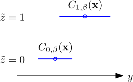
Figure 2: Counterfactual analysis of units with covariates $\mathbf{x}$ assigned to different exposures $\tilde{z}$. Outcome predictions $\widehat{\mu}_{0}(\mathbf{x})$ and $\widehat{\mu}_{1}(\mathbf{x})$ are denoted by circles. The prediction intervals (PIs) $C_{0,\beta}(\mathbf{x})$ and $C_{1,\beta}(\mathbf{x})$ (lines) incorporate the outcomes with a coverage of $100\%\beta$. Together the PIs enable an intuitive assessment of the counterfactual outcomes. Below we propose using the PIs to quantify how separable the outcomes are under different exposures.

A major challenge is obtaining PIs that are valid when the data-generating process is unknown. Here we consider the general conformal approach of [26, 27] to construct PIs with valid coverage properties in distribution-free manner. Each point in the interval is then constructed by re-fitting the predictor for the corresponding exposure group. This becomes computationally prohibitive using complex tree-based models or fitting methods that require parameter tuning, especially when $\mathbf{x}$ is high-dimensional. This obstacle is circumvented using the method proposed below.

Our contributions in this paper are the following. We propose the use of prediction intervals for covariate-specific counterfactual analysis of each exposure type and define a measure of their relative impact that provides additional information to merely comparing $\widehat{\mu}_{0}(\mathbf{x})$ and $\widehat{\mu}_{1}(\mathbf{x})$. We then learn sparse predictor models $\widehat{\mu}_{\tilde{z}}(\mathbf{x})$, with corresponding PIs $C_{\tilde{z}}(\mathbf{x})$, that automatically adapt to nonlinearities by leveraging the computational properties of the Spice predictor approach [28]. This obviates the need for cross-validation or other tuning techniques. Since the conformal PIs also exhibit marginal coverage properties, even when lacking a correctly specified model of the data-generating process, the resulting method provides a model-robust means of counterfactual analysis.

Notation: $\|\cdot\|_{1}$ and $\odot$ denote the $\ell_{1}$-norm and Hadamard product. The cardinality of a set $\mathcal{D}$ is $|\mathcal{D}|$. The operator $\operatorname{col}\{\mathbf{x}_{1},\dots,\mathbf{x}_{k}\}$ stacks all elements into a single column vector. $\widehat{\operatorname{E}}[f(\mathbf{x},y)|\tilde{z}]=|\mathcal{D}_{\tilde{z}}|^{-1}\sum_{i}f(\mathbf{x}_{i},y_{i})$ is the empirical mean of $f(\mathbf{x},y)$ over all pairs $(\mathbf{x},y)$ in $\mathcal{D}_{\tilde{z}}$.

Remark: Code for the proposed method is available at https://github.com/dzachariah/counterfactual.

II Counterfactual prediction method

A predictive approach to counterfactual analysis is readily generalized to multiple exposure types $z\in\{0,\dots,K-1\}$. We illustrate this as we proceed to define a measure of the separability of counterfactual outcomes under different exposures.

II-A Counterfactual confidence

Consider an observational study with $K=3$ exposure types and a scalar covariate $x$, as illustrated in Fig. 3. For a given $x$, let $\widehat{\mu}_{\tilde{z}}(x)$ and prediction intervals $C_{\tilde{z},\beta}(x)$ be the counterfactual prediction and PI for each exposure $\tilde{z}\in\{0,1,2\}$. We propose the following measure of the impact of exposures on the outcomes.

Definition 1.

A covariate-specific comparison between predicted outcomes for exposures $\tilde{z}$ and $z$ is said to have $100\beta$% counterfactual confidence, where $\beta$ is the largest value for which their PIs do not overlap. That is, the PIs are mutually exclusive

$$C_{\tilde{z},\beta}(\mathbf{x})\cap C_{z,\beta}(\mathbf{x})=\emptyset.$$ (1)

A high confidence asserts that the counterfactual outcomes are highly separable and thus the impact of the exposures are more distinctive. This provides additional information to the size of the exposure effect measured as $\widehat{\mu}_{\tilde{z}}(\mathbf{x})-\widehat{\mu}_{z}(\mathbf{x})$.

In Fig. 3 we see that for a unit with covariate $x=-1$, the counterfactual confidence when comparing exposures $1$ and $2$ is greater than $90\%$, indicating highly separable outcomes. The confidences for the pairwise are tabulated pairwise below for covariate $x=-1$ (left) and $x=2$ (right):

$\tilde{z}$	$0$	$1$
1	81%	–
2	64%	96%

$\tilde{z}$	$0$	$1$
1	24%	–
2	45%	58%

It is seen that for $x=-1$, the separability of counterfactual outcomes can be asserted with greater confidence than for $x=2$. This is corroborated by comparing the datasets shown in Fig. 3.

   

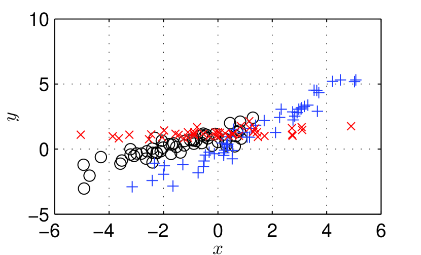
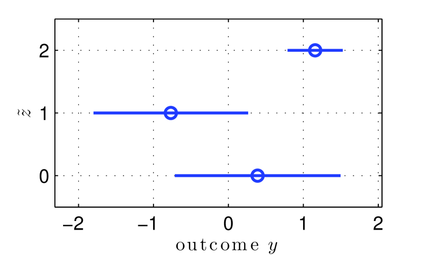
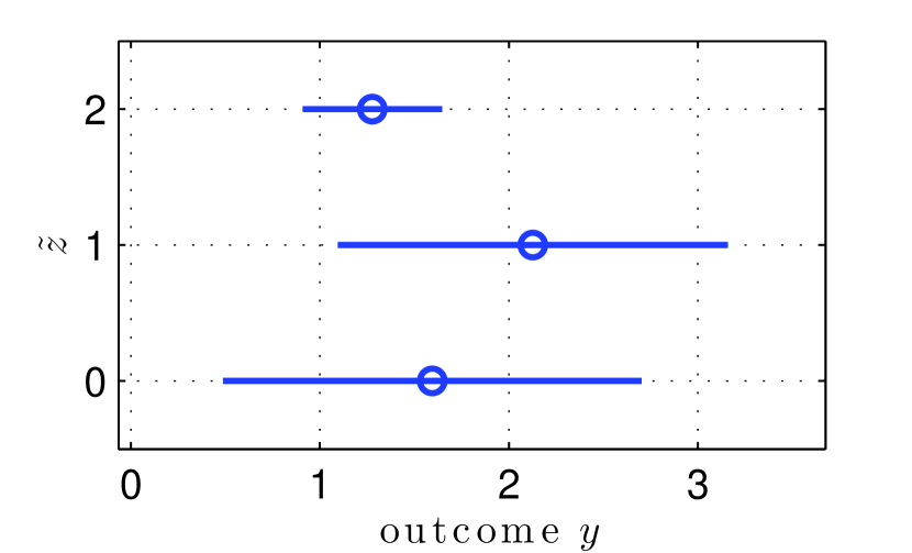
Figure 3: Counterfactual analysis with $K=3$ exposure types and scalar covariate $x$, using method proposed on subsequent sections. Left: Datasets $\mathcal{D}_{\tilde{z}}$ for exposures $\tilde{z}=0$ ($\circ$), $1$ ($+$) and $2$ ($\times$). The resulting predictions $\widehat{\mu}_{\tilde{z}}(x)$ along with $90\%$-intervals $C_{\tilde{z},0.90}(x)$. Center: $x=-1$. Right: $x=2$.

II-B Conformal prediction intervals

Consider a regression model class

$$\mathcal{M}_{\mu}=\Big{\{}\mu:\mu(\mathbf{x})=\boldsymbol{\phi}^{\top}(\mathbf{x})\mathbf{w},\;\mathbf{w}\in\mathbb{R}^{p+1}\Big{\}},$$

parameterized by $\mathbf{w}$. In subsection II-C, we specify a flexible regressor vector $\boldsymbol{\phi}(\mathbf{x})$ that adapts to nonlinearities in the data. When the model class is well-specified it includes the unknown mean function $\mu_{z}(\mathbf{x})\in\mathcal{M}_{\mu}$.

To learn a model in $\mathcal{M}_{\mu}$ from $\mathcal{D}_{z}$, we build upon the tuning-free Spice-method [28] where the learned weights are defined as

$$\widehat{\mathbf{w}}\>=\>\operatorname*{arg\,min}_{\mathbf{w}}\>\sqrt{\widehat{\operatorname{E}}\big{[}\>|y-\boldsymbol{\phi}^{\top}(\mathbf{x})\mathbf{w}|^{2}\>\big{|}\>\tilde{z}\>\big{]}}+\>\|\boldsymbol{\varphi}\odot\mathbf{w}\|_{1},$$ (2)

and the elements of $\boldsymbol{\varphi}$ are given by

$$\varphi_{j}=\begin{cases}\sqrt{\frac{\widehat{\operatorname{E}}\big{[}\>\phi^{2}_{j}(\mathbf{x})\>|\>\tilde{z}\>\big{]}}{|\mathcal{D}_{\tilde{z}}|}},&j=1,\dots,p\\ 0,&j=0.\end{cases}$$

The solution (2) can be computed sequentially for each sample in $\mathcal{D}_{\tilde{z}}$, using a coordinate descent algorithm with a runtime that scales as $\mathcal{O}(|\mathcal{D}_{\tilde{z}}|p^{2})$. We now leverage this property for the construction of conformal PIs.

The principle behind general conformal prediction can be described as follows [26, 27]: For the covariate of interest $\mathbf{x}$, consider a new sample $(\mathbf{x},\widetilde{y})$ where $\widetilde{y}$ is a variable. Then quantify how well this sample conforms to the observed data $\mathcal{D}_{\tilde{z}}$ via the learned model (2). All points $\widetilde{y}$ that conform well, form a prediction interval. The conformity is quantified by including $(\mathbf{x},\widetilde{y})$ in the learned model (2), which is achieved by a sequential update in $\mathcal{O}(p^{2})$. Then, following [29], we define a measure

$$\pi(\widetilde{y})=\frac{1}{|\mathcal{D}_{\tilde{z}}|+1}\Big{(}1+\sum_{i}I\big{\{}r_{i}\leq|\widetilde{y}-\boldsymbol{\phi}^{\top}(\mathbf{x})\widehat{\mathbf{w}}|\big{\}}\Big{)},$$ (3)

where $r_{i}=|y_{i}-\boldsymbol{\phi}^{\top}(\mathbf{x}_{i})\widehat{\mathbf{w}}|$ is the $i$th fitted residual and $I\{\cdot\}$ is the indicator function. The measure is bounded between 0 and 1, where lower values correspond to higher conformity. We construct $C_{\tilde{z},\beta}(\mathbf{x})$ by varying $\widetilde{y}$ over a set of grid points $\widetilde{\mathcal{Y}}$, as summarized in Algorithm 1. By leveraging the computational properties of the learning method, the prediction interval is computed with a total runtime of $\mathcal{O}(|\widetilde{\mathcal{Y}}|p(p+|\mathcal{D}_{\tilde{z}}|))$. The range of $\widetilde{\mathcal{Y}}$ is set to exceed that of the outcomes in the observed dataset. A point prediction $\widehat{\mu}_{\tilde{z}}(\mathbf{x})$ is obtained as the minimizer of $\pi(\widetilde{y})$.

Algorithm 1 : Conformal prediction interval

1:Input: covariate $\mathbf{x}$, target coverage $\beta$ and data $\mathcal{D}_{\tilde{z}}$

2:for  all $\widetilde{y}\in\widetilde{\mathcal{Y}}$ do

3:     Update $\widehat{\mathbf{w}}$ using $(\mathbf{x},\widetilde{y})$

4:     Compute $\{r_{i}\}$ and $\pi(\widetilde{y})$ in (3)

5:end for

6:Output: $C_{\tilde{z},\beta}(\mathbf{x})=\big{\{}\widetilde{y}\in\widetilde{\mathcal{Y}}\>:\>(n+1)\pi(\widetilde{y})\leq\lceil\beta(n+1)\rceil\big{\}}$

Despite the fact that no dispersion model of the data generating process is required, the resulting prediction intervals exhibit valid coverage properties. When the model class $\mathcal{M}_{\mu}$ is well-specified, the interval exhibits asymptotic conditional coverage, that is,

$$\Pr\big{\{}\>y\in C_{\tilde{z},\beta}(\mathbf{x})\>\bigl{|}\>\mathbf{x},\tilde{z}\>\big{\}}\>=\>\beta+o_{P}(1),$$

under certain regularity conditions [29, thm. 6.2]. More generally, $C_{\tilde{z},\beta}(\mathbf{x})$ is calibrated to ensure marginal coverage [29, thm. 2.1]

$$\Pr\big{\{}\>y\in C_{\tilde{z},\beta}(\mathbf{x})\>\big{|}\>\tilde{z}\>\big{\}}\>\geq\>\beta.$$

Note that this does not require a well-specified model class $\mathcal{M}_{\mu}$. In other words, the more accurate the learned prediction model, the tighter the prediction interval but its marginal coverage property remains not matter if the model is correct or not. This confers a robustness property to the proposed inference method in cases when $\mu_{\tilde{z}}(\mathbf{x})\not\in\mathcal{M}_{\mu}$.

II-C Sparse additive predictor models

To learn accurate prediction models, we now turn to the specification of the regressor vector in $\mathcal{M}_{\mu}$. Let $d$ denote the dimension of $\mathbf{x}$ and consider the additive model

$$\boldsymbol{\phi}(\mathbf{x})=\operatorname{col}\big{\{}1,\>\boldsymbol{\psi}_{1}(x_{1}),\>\dots,\>\boldsymbol{\psi}_{d}(x_{d})\big{\}},$$

which enables interpretable component-wise predictors [21]. When a covariate $x$ is categorical, we use a standard basis vector $\boldsymbol{\psi}(x)\equiv\mathbf{e}_{k}$ for category $k\neq 0$ and $\mathbf{0}$ when $k=0$. In the case of binary categories, we simply have $\boldsymbol{\psi}(x)\equiv 1$.

For noncategorical covariates $x$, such as continuous or count variables, however, we propose a data-adaptive piecewise linear model. Let the empirical quantile function be

$$\widehat{F}^{-1}(q)=\inf\big{\{}x:\widehat{F}(x)\leq q\big{\}},$$

where $\widehat{F}(x)$ is the empirical cumulative density function of $x$ obtained from the full observational data $\mathcal{D}$. Then we specify the model for $x$ by the $m$-dimensional vector

$$[\boldsymbol{\psi}(x)]_{k}=\begin{cases}(x-c_{k})_{+},&k=1,\dots,m-1\\ (x-c_{k})_{+}I\{x\leq c_{k+1}\}&\\ \>+\>c_{k+1}I\{x>c_{k+1}\},&k=m\end{cases}$$

where $m$ is a specified number of knots or breakpoints defined as $c_{k}=\widehat{F}^{-1}(\frac{k-1}{m})$. The resulting model yields finer resolution line segments where data density is high and is capable of capturing continuous nonlinear responses with respect to $x$.

The regularization term in (2) leads to sparse solutions and thus the learning method yields a set of sparse additive predictor models $\widehat{\mu}_{\tilde{z}}(\mathbf{x})=\widehat{\mu}_{\tilde{z}}(x_{1})+\dots+\widehat{\mu}_{\tilde{z}}(x_{d})$ with nonlinear responses in a data-adaptive manner, cf. [30]. Moreover, the method takes into account the amount of data observed within each line segment for each exposure type, and controls the model complexity accordingly. This mitigates overfitting when there is unequal training data or covariate imbalances across exposure types, cf. [24].

The integer $m$ determines the maximum resolution of the nonlinear model. A high $m$ enables higher predictive accuracy provided enough data is available to learn the nonlinear response. For instance, suppose $n$ denotes the size of the smallest dataset $\mathcal{D}_{\tilde{z}}$ and $d^{\prime}$ and $d^{\prime\prime}$ denote the number of binary and continuous covariates, respectively. Then $p=d^{\prime}+md^{\prime\prime}$ and a natural upper limit is $m\leq\max(\lceil\frac{n-d^{\prime}}{d^{\prime\prime}}\rfloor,1)$.

III Numerical experiments

In this section we demonstrate the proposed counterfactual prediction approach by means of three examples. In the following examples, we consider $K=2$ exposure types.

III-A Nonlinear effects

We consider the example in [22], which allows for a comparison with both tree-based and linear models. For each unit, the exposure $z$ is assigned with equal probability. Then the covariate $x$ (with $d=1$) is drawn as

$$x|(z=0)\sim\mathcal{N}(40,10^{2})\quad\text{and}\quad x|(z=1)\sim\mathcal{N}(20,10^{2})$$

and the counterfactual outcomes as

$$\begin{split}y(0)|x&\sim\mathcal{N}(72+3\sqrt{|x|},1)\quad\text{and}\\ y(1)|x&\sim\mathcal{N}(90+\exp(0.06x),1).\end{split}$$ (4)

A simulated observational dataset $\mathcal{D}$ with $n=120$ is illustrated in Fig. 4. To obtain the predictions in the figure, we use $m=10$. For a unit with covariate $x=30$, as an example, we note that $\widehat{\mu}_{1}(30)$ is larger than $\widehat{\mu}_{0}(30)$ and that both confidence intervals are tight, as is expected by inspecting the data generating process (4) at the given covariate. In addition, the counterfactual confidence is found to be greater than 90%, indicating a highly separable counterfactual outcomes as expected.

To illustrate the robustness property of the prediction intervals, we repeat the experiment using 1000 Monte Carlo simulations. For each simulation, we generate new data $\mathcal{D}$ and also draw a new unit from both exposure groups. For a unit with exposure $z=0$, the outcome is found to belong to interval $C_{0,\beta}(x)$ with probability 0.918 when $\beta=0.90$. Similarly, for exposure $z=1$, the outcome is contained in the interval $C_{1,\beta}(x)$ with probability 0.907. This coverage property holds eventhough the mean function does not belong to $\mathcal{M}_{\mu}$.

 

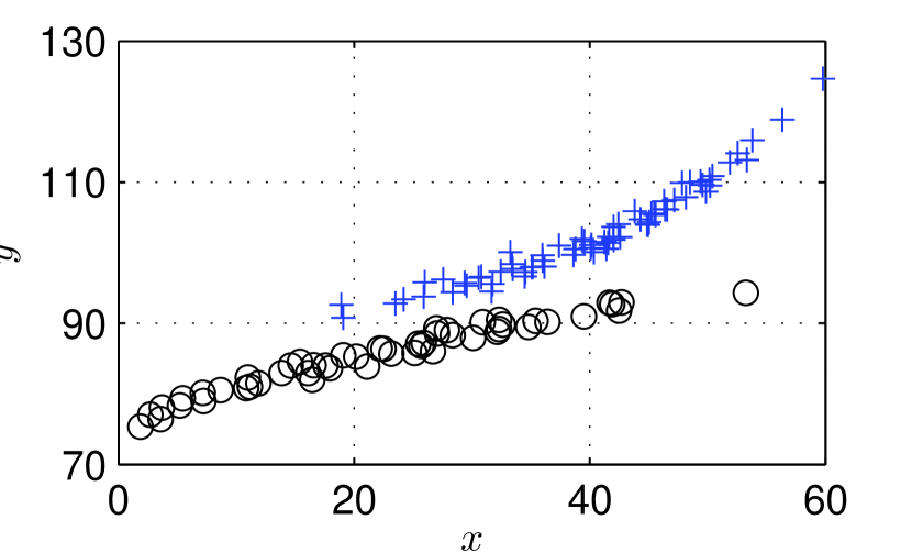
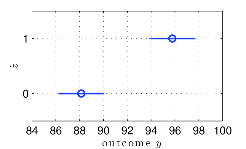
Figure 4: Left: Dataset $\mathcal{D}$ with $n=120$ samples. Exposures $\tilde{z}=0$ ($\circ$) and $1$ ($+$). Right: Predictions with $90\%$-prediction intervals at $x=30$.

III-B High-dimensional covariates

The desire to include all potential confounders in the covariate vector $\mathbf{x}$, may lead in many applications to dimensions $d$ that can be larger than $n$ [16]. To address this issue, we simulate an experimental setting with $d=200$ covariates but only $n=100$ samples. Naturally, we have $m=1$. The exposures $z=0$ and $z=1$ are assigned with probabilities 0.6 and 0.4, respectively. The covariates are drawn as

$$\mathbf{x}|(z=0)\sim\mathcal{N}(\mathbf{0},\boldsymbol{\Sigma}_{0})\quad\text{and}\quad\mathbf{x}|(z=1)\sim\mathcal{N}(\mathbf{0},\boldsymbol{\Sigma}_{1}),$$

where $\boldsymbol{\Sigma}_{0}$ and $\boldsymbol{\Sigma}_{1}$ are randomly generated covariance matrices with unit trace. The matrices have numerical rank $150$ and are constructed using outer products of Gaussian vectors. This generates highly correlated covariates, as is typical in real applications. The counterfactual outcomes are generated as

$$\begin{split}y(0)|\mathbf{x}&\sim\mathcal{N}(x_{1}+5x_{10}+5x_{20}+0.5,\;0.5^{2})\quad\text{and}\\ y(1)|\mathbf{x}&\sim\mathcal{N}(x_{1}+x_{10}-x_{30},\;0.5^{2}).\end{split}$$ (5)

However, this is not a problem for the learning method which automatically prunes away irrelevant covariates due to the adaptive regularization in (2).

A simulated observational dataset $\mathcal{D}$ is shown in Fig. 5. We also illustrate the predicted outcomes for a unit with all covariates equal to one, $\mathbf{x}=\mathbf{1}$. We observe that $\widehat{\mu}_{0}(\mathbf{1})$ is considerably larger than $\widehat{\mu}_{1}(\mathbf{1})$, also when taking into account the prediction intervals. This is consistent with the data generating process (5) evaluated at the fixed $\mathbf{x}$. The interval for exposure $z=0$ is also seen to be significantly wider than that for exposure $z=1$, reflecting the larger uncertainty of the predicted outcome. In this case it is possible to assert counterfactual confidence greater than 90%.

We repeat this experiment as well to validate the coverage properties of the intervals, using 1000 Monte Carlo simulations. For each simulation, we generate new data $\mathcal{D}$ and also draw a new unit from both exposure groups. For a unit with exposure $z=0$, the outcome is found to be contained in interval $C_{0,\beta}(\mathbf{x})$ with probability 0.921 when $\beta=0.90$. Similarly, for exposure $z=1$, the outcome is contained in the interval $C_{1,\beta}(\mathbf{x})$ with probability 0.915.

 

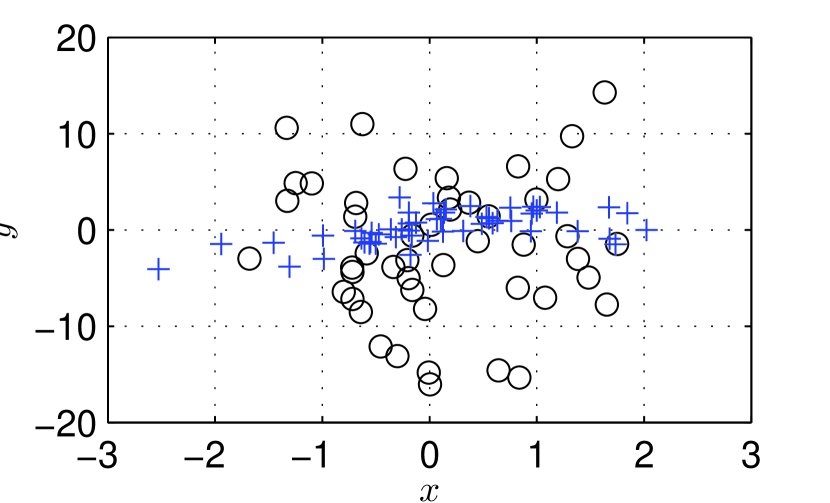
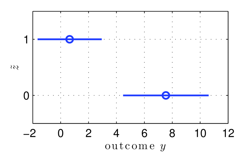
Figure 5: Left: Dataset $\mathcal{D}$ with $n=100$ samples. Only one covariate, $x_{1}$, is shown for the sake of two-dimensional visualization. Exposures $\tilde{z}=0$ ($\circ$) and $1$ ($+$). Right: Predictions with $90\%$-prediction intervals at $\mathbf{x}=\mathbf{1}$.

III-C Schooling data

Following the example in [31], we assess the effect of schooling on income for adults in the US born in the 1930s, using data from [32]. The observed outcome $y$ is the weekly earnings (on a logarithmic scale) of a subject in 1970. Each individual is subject to one of two exposures: $z=1$ corresponds to receiving 12 years of schooling or more and $z=0$ corresponds to receiving less than 12 years. We consider 26 binary covariates in $\mathbf{x}$. Ten covariates indicate the year of birth 1930-1939, and eight indicate the census region. In addition, eight indicators represent ethnic identification, marital status and whether or not the subject lives in the central city of a metropolitan area. The observational study consists of $n=329~{}509$ samples. (See [31] for details.)

Discrete covariates can be partitioned into separate subgroups, and a direct inference approach would be to estimate the average outcomes of exposures 0 and 1 for each group. However, the number of subgroups grows quickly and there are not sufficient samples in the dataset $\mathcal{D}$ for each subgroup and exposure. Therefore we apply the proposed method. The predicted outcomes are illustrated for subjects in different covariate groups in Fig 6. All subjects in these subgroups were born in the same year and came from the same region. The prediction interval widths are likely to be affected by the very coarse division of schooling used here, since $z=0$ includes 0 to 11 years of schooling, which is a substantial variation, while $z=1$ includes 12 years and more.

The three subgroups are $\mathbf{x}_{1}$: Caucasian, unmarried and not in a major city, $\mathbf{x}_{2}$: Caucasian, married and in a major city, and $\mathbf{x}_{3}$: African-American, married, and in a major city. Given that the units are logarithmic, the differences of predicted earnings, $\widehat{\mu}_{1}(\mathbf{x})-\widehat{\mu}_{0}(\mathbf{x})$, correspond to +52%, +26% and +39% of weekly earnings, for $\mathbf{x}_{1}$, $\mathbf{x}_{2}$ and $\mathbf{x}_{3}$, respectively. This means that the inferred effect of schooling is greatest for $\mathbf{x}_{1}$ while considerably less for $\mathbf{x}_{2}$. The prediction intervals in Fig. 6 suggest, however, that there is a considerable dispersion of the outcomes. The predicted outcome of schooling has a counterfactual confidence of 33%, 20% and 25% for the three subgroups. Thus for subgroup $\mathbf{x}_{2}$, schooling not only exhibits the lowest predicted gains but also the least separable counterfactual outcomes can be asserted. The opposite is true for subgroup $\mathbf{x}_{1}$.

The findings appear to be consistent with features of US society in the 1970s: a Caucasian person in a major city with a family was expected to have greater access to economic opportunities, such that schooling experience mattered less to earnings. For the unmarried counterpart who lived outside of the major city, such alternative opportunities were fewer so that schooling could have a more significant impact. An African-American person in a major city with a family represents an intermediate case.

   

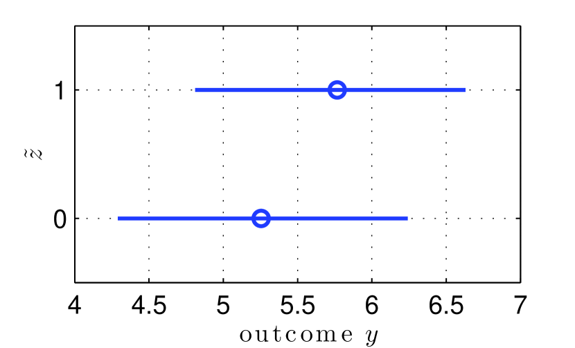
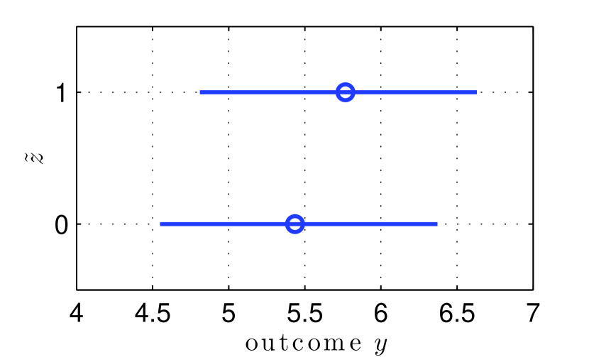
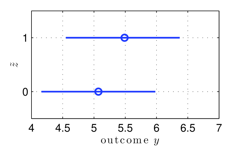
Figure 6: Counterfactual analysis of schooling ($\tilde{z}$) and weekly earnings ($y$, in logarithmic units) using $90\%$-prediction intervals. Left: Caucasian, unmarried and not in major city. Center: Caucasian, married and in city. Right: African-american, married and in city.

IV Conclusions

We have developed a new method for counterfactual analysis using observational data based on prediction intervals. The intervals were used to define a measure of relative separability of counterfactual outcomes under different exposures. This takes into account the dispersions of the outcomes and provides additional information to the difference between predictions.

The intervals were constructed in a distribution-free and model-robust manner based on the general conformal prediction approach. The computational obstacles of this approach were circumvented by leveraging properties of a tuning-free method that learns sparse additive predictor models for counterfactual outcomes. We demonstrated the method using both real and synthetic data.

References

- [1] M. A. Hernán and J. M. Robins, Causal Inference. Chapman & Hall/CRC, 2018. forthcoming.
- [2] S. L. Morgan and C. Winship, Counterfactuals and causal inference. Cambridge University Press, 2014.
- [3] J. Neyman, “Sur les applications de la théorie des probabilités aux experiences agricoles: Essai des principes,” Roczniki Nauk Rolniczych, vol. 10, pp. 1–51, 1923.
- [4] D. B. Rubin, “Estimating causal effects of treatments in randomized and nonrandomized studies.,” Journal of Educational Psychology, vol. 66, no. 5, p. 688, 1974.
- [5] J. Pearl, Causality. Cambridge University Press, 2009.
- [6] J. Pearl et al., “Causal inference in statistics: An overview,” Statistics surveys, vol. 3, pp. 96–146, 2009.
- [7] A. Sjölander, “The language of potential outcomes,” in Causality: Statistical Perspectives and Applications, John Wiley & Sons, 2012.
- [8] S. Greenland, “Causal inference as a prediction problem: Assumptions, identification and evidence synthesis,” in Causality: Statistical Perspectives and Applications, John Wiley & Sons, 2012.
- [9] J. Peters, D. Janzing, and B. Schölkopf, Elements of Causal Inference: Foundations and Learning Algorithms. MIT Press, 2017.
- [10] T. S. Richardson and J. M. Robins, “Single world intervention graphs: a primer,” in Second UAI workshop on causal structure learning, Bellevue, Washington, 2013.
- [11] G. W. Imbens, “Nonparametric estimation of average treatment effects under exogeneity: A review,” Review of Economics and statistics, vol. 86, no. 1, pp. 4–29, 2004.
- [12] L. Wasserman, All of Statistics: A Concise Course in Statistical Inference. Springer Texts in Statistics, Springer New York, 2004.
- [13] G. W. Imbens and D. B. Rubin, Causal inference in statistics, social, and biomedical sciences. Cambridge University Press, 2015.
- [14] J. M. Robins and Y. Ritov, “Toward a curse of dimensionality appropriate (coda) asymptotic theory for semi-parametric models,” Statistics in medicine, vol. 16, no. 3, pp. 285–319, 1997.
- [15] A. Belloni, V. Chernozhukov, and C. Hansen, “Inference on treatment effects after selection among high-dimensional controls,” The Review of Economic Studies, vol. 81, no. 2, pp. 608–650, 2014.
- [16] M. H. Farrell, “Robust inference on average treatment effects with possibly more covariates than observations,” Journal of Econometrics, vol. 189, no. 1, pp. 1–23, 2015.
- [17] V. Chernozhukov, D. Chetverikov, M. Demirer, E. Duflo, C. Hansen, and W. Newey, “Double/debiased/neyman machine learning of treatment effects,” arXiv preprint arXiv:1701.08687, 2017.
- [18] P. M. Rothwell, “Can overall results of clinical trials be applied to all patients?,” The Lancet, vol. 345, no. 8965, pp. 1616–1619, 1995.
- [19] D. M. Kent and R. A. Hayward, “Limitations of applying summary results of clinical trials to individual patients: the need for risk stratification,” Jama, vol. 298, no. 10, pp. 1209–1212, 2007.
- [20] J. Weiss, F. Kuusisto, K. Boyd, J. Liu, and D. Page, “Machine learning for treatment assignment: Improving individualized risk attribution,” in AMIA Annual Symposium Proceedings, vol. 2015, p. 1306, American Medical Informatics Association, 2015.
- [21] T. Hastie, R. Tibshirani, and J. Friedman, The Elements of Statistical Learning: Data Mining, Inference, and Prediction. Springer Series in Statistics, Springer New York, 2013.
- [22] J. L. Hill, “Bayesian nonparametric modeling for causal inference,” Journal of Computational and Graphical Statistics, vol. 20, no. 1, pp. 217–240, 2011.
- [23] S. Wager and S. Athey, “Estimation and inference of heterogeneous treatment effects using random forests,” Journal of the American Statistical Association, no. just-accepted, 2017.
- [24] S. Künzel, J. Sekhon, P. Bickel, and B. Yu, “Meta-learners for estimating heterogeneous treatment effects using machine learning,” arXiv preprint arXiv:1706.03461, 2017.
- [25] S. Geisser, Predictive inference. CRC Press, 1993.
- [26] V. Vovk, A. Gammerman, and G. Shafer, Algorithmic learning in a random world. Springer Science & Business Media, 2005.
- [27] V. Balasubramanian, S.-S. Ho, and V. Vovk, Conformal prediction for reliable machine learning: Theory, Adaptations and applications. Newnes, 2014.
- [28] D. Zachariah, P. Stoica, and T. B. Schön, “Online learning for distribution-free prediction,” arXiv preprint arXiv:1703.05060, 2017.
- [29] J. Lei, M. G’Sell, A. Rinaldo, R. J. Tibshirani, and L. Wasserman, “Distribution-free predictive inference for regression,” Journal of the American Statistical Association, no. just-accepted, 2017.
- [30] P. Ravikumar, H. Liu, J. Lafferty, and L. Wasserman, “Spam: Sparse additive models,” in Proceedings of the 20th International Conference on Neural Information Processing Systems, pp. 1201–1208, Curran Associates Inc., 2007.
- [31] J. Esarey, “Causal inference with observational data,” in Analytics, Policy, and Governance, Yale University Press, 2017.
- [32] J. D. Angrist and A. B. Krueger, “Does compulsory school attendance affect schooling and earnings?,” The Quarterly Journal of Economics, vol. 106, no. 4, pp. 979–1014, 1991.