On Packet Scheduling with Adversarial Jamming and Speedup

Abstract

In Packet Scheduling with Adversarial Jamming packets of arbitrary sizes arrive over time to be transmitted over a channel in which instantaneous jamming errors occur at times chosen by the adversary and not known to the algorithm. The transmission taking place at the time of jamming is corrupt, and the algorithm learns this fact immediately. An online algorithm maximizes the total size of packets it successfully transmits and the goal is to develop an algorithm with the lowest possible asymptotic competitive ratio, where the additive constant may depend on packet sizes.

Our main contribution is a universal algorithm that works for any speedup and packet sizes and, unlike previous algorithms for the problem, it does not need to know these parameters in advance. We show that this algorithm guarantees 1-competitiveness with speedup 4, making it the first known algorithm to maintain 1-competitiveness with a moderate speedup in the general setting of arbitrary packet sizes. We also prove a lower bound of $\phi+1\approx 2.618$ on the speedup of any 1-competitive deterministic algorithm, showing that our algorithm is close to the optimum.

Additionally, we formulate a general framework for analyzing our algorithm locally and use it to show upper bounds on its competitive ratio for speedups in $[1,4)$ and for several special cases, recovering some previously known results, each of which had a dedicated proof. In particular, our algorithm is 3-competitive without speedup, matching both the (worst-case) performance of the algorithm by Jurdzinski et al. [10] and the lower bound by Anta et al. [1].

1 Introduction

We study an online packet scheduling model recently introduced by Anta et al. [1] and extended by Jurdzinski et al. [10]. In our model, packets of arbitrary sizes arrive over time and they are to be transmitted over a single communication channel. The algorithm can schedule any packet of its choice at any time, but cannot interrupt its subsequent transmission; in the scheduling jargon, there is a single machine and no preemptions. There are, however, instantaneous jamming errors or faults at times chosen by the adversary, which are not known to the algorithm. A transmission taking place at the time of jamming is corrupt, and the algorithm learns this fact immediately. The packet whose transmission failed can be retransmitted immediately or at any later time, but the new transmission needs to send the whole packet, i.e., the algorithm cannot resume a transmission that failed.

The objective is to maximize the total size of packets successfully transmitted. In particular, the goal is to develop an online algorithm with the lowest possible competitive ratio, which is the asymptotic worst-case ratio between the total size of packets in an optimal offline schedule and the total size of packets completed by the algorithm on a large instance. (See the next subsection for a detailed explanation of competitive analysis.)

We focus on algorithms with resource augmentation, namely on online algorithms that transmit packets $s\geq 1$ times faster than the offline optimum solution they are compared against; such algorithm is often said to be speed-$s$, running at speed $s$, or having a speedup of $s$. As our problem allows constant competitive ratio already at speed $1$, we consider the competitive ratio as a function of the speed. This deviates from previous work, which focused on the case with no speedup or on the speedup sufficient for ratio 1, ignoring intermediate cases.

1.1 Competitive Analysis and its Extensions

Competitive analysis focuses on determining the competitive ratio of an online algorithm. The competitive ratio coincides with the approximation ratio, i.e., the supremum over all valid instances $I$ of $\textsf{OPT\/}(I)/\textsf{ALG\/}(I)$, which is the ratio of the optimum profit to the profit of an algorithm ALG on instance $I$. This name, as opposed to approximation ratio, is used for historical reasons, and stresses that the nature of the hardness at hand is not due to computational complexity, but rather the online mode of computation, i.e., processing an unpredictable sequence of requests, completing each without knowing the future. Note that the optimum solution is to the whole instance, so it can be thought of as being determined by an algorithm that knows the whole instance in advance and has unlimited computational power; for this reason, the optimum solution is sometimes called “offline optimum”. Competitive analysis, not yet called this way, was first applied by Sleator and Tarjan to analyze list update and paging problems [19]. Since then, it was employed to the study of many online optimization problems, as evidenced by (now somewhat dated) textbook by Borodin and El-Yaniv [6]. A nice overview of competitive analysis and its many extensions in the scheduling context, including intuitions and meaning can be found in a survey by Pruhs [17].

1.1.1 Asymptotic Ratio and Additive Constant

In some problems of discrete nature, such as bin packing or various coloring problems, it appears that the standard notion of competitive analysis is too restrictive. The problem is that in order to attain competitive ratio relatively close to $1$ (or even any ratio), an online algorithm must behave in a predictable way when the current optimum value is still small, which makes the algorithms more or less trivial and the ratio somewhat large. To remedy this, the “asymptotic competitive ratio” is often considered, which means essentially that only instances with a sufficiently large optimum value are considered. This is often captured by stating that an algorithm is $R$-competitive if (in our convention) there exists a constant $c$ such that $R\cdot\textsf{ALG\/}(I)+c\geq\textsf{OPT\/}(I)$ holds for every instance $I$. The constant $c$ is typically required not to depend on the class of instances considered, which makes sense for aforementioned problems where the optimum value corresponds to the number of bins or colors used, but is still sometimes too restrictive.

This is the case in our problem. Specifically, using an example we show that a deterministic algorithm running at speed $1$ can be (constant) competitive only if the additive term in the definition of the competitive ratio depends on the values of the packet sizes, even if there are only two packet sizes. Suppose that a packet of size $\ell$ arrives at time $0$. If the algorithm starts transmitting it immediately at time $0$, then at time $\varepsilon>0$ a packet of size $\ell-2\epsilon$ arrives, the next fault is at time $\ell-\varepsilon$ and then the schedule ends, i.e., the time horizon is at $T=\ell-\varepsilon$. Thus the algorithm does not complete the packet of size $\ell$, while the adversary completes a slightly smaller packet of size $\ell-2\epsilon$. Otherwise, the algorithm is idle till some time $\varepsilon>0$, no other packet arrives and the next fault is at time $\ell$, which is also the time horizon. In this case, the packet of size $\ell$ is completed in the optimal schedule, while the algorithm completes no packet again.

1.1.2 Resource Augmentation

Last but not least, some problems do not admit competitive algorithms at all or yield counterintuitive results. Again, our problem is an example of the former kind if no additive constant depending on packet sizes is allowed (cf. aforementioned example), whereas the latter can be observed in the paging problem, where the optimum ratio equals the cache size, seemingly suggesting that the larger the cache size, the worse the performance, regardless of the caching policy. Perhaps for this reason, already Sleator and Tarjan [19] considered resource augmentation for paging problem, comparing an online algorithm with cache capacity $k$ to the optimum with cache capacity $h\leq k$. Yet again, they were ahead of the time: resource augmentation was re-introduced and popularized in scheduling problems by Kalyanasundaram and Pruhs [11], and the name itself coined by Phillips et al. [16], who also considered scheduling.

We give a brief overview of some of the work on resource augmentation in online scheduling, focusing on interesting open problems. As mentioned before, Kalyanasundaram and Pruhs [11] introduced resource augmentation. Among other results they proved that a constant competitive ratio is possible with a constant speedup for a preemptive variant of real-time scheduling where each job has a release time, deadline, processing time and a weight and the objective is to maximize the weight of jobs completed by their deadlines on a single machine. Subsequently resource augmentation was applied in various scenarios. Of the most relevant for us are those that considered algorithms with speedup that are 1-competitive, i.e., as good as the optimum. We mention two models that still contain interesting open problems.

For real-time scheduling, Phillips et al. [16] considered the underloaded case in which there exists a schedule that completes all the jobs. It is easy to see that on a single machine, the Earliest-Deadline First (EDF) algorithm is then an optimal online algorithm. Phillips et al. [16] proved that EDF on $m$ machines is 1-competitive with speedup $2-1/m$. (Here the weights are not relevant.) Intriguingly, finding a 1-competitive algorithm with minimal speedup for $m>1$ is wide open: It is known that speedup at least $6/5$ is necessary, it has been conjectured that speedup $e/(e-1)$ is sufficient, but the best upper bound proven is $2-2/(m+1)$ from [15]. See Schewior [18] for more on this problem.

Later these results were extended to real-time scheduling of overloaded systems, where for uniform density (i.e., weight equal to processing time) Lam et al. [14] have shown that a variant of EDF with admission control is 1-competitive with speedup 2 on a single machine and with speedup 3 on more machines. For non-uniform densities, the necessary speedup is a constant if each job is tight (its deadline equals its release time plus its processing time) [12]. Without this restriction it is no longer constant, depending on the ratio $\xi$ of the maximum and minimum weight. It is known that it is at least $\Omega(\log\log\xi)$ and at most $\mathcal{O}(\log\xi)$ [7, 14]; as far as we are aware, closing this gap is still an open problem.

1.2 Previous and Related Results

The model was introduced by Anta et al. [1], who resolved it for two packet sizes: If $\gamma>1$ denotes the ratio of the two sizes, then the optimum competitive ratio for deterministic algorithms is $(\gamma+\lfloor\gamma\rfloor)/\lfloor\gamma\rfloor$, which is always in the range $[2,3)$. This result was extended by Jurdzinski et al. [10], who proved that the optimum ratio for the case of multiple (though fixed) packet sizes is given by the same formula for the two packet sizes which maximize it.

Moreover, Jurdzinski et al. [10] gave further results for divisible packet sizes, i.e., instances in which every packet size divides every larger packet size. In particular, they proved that on such instances speed $2$ is sufficient for $1$-competitiveness in the resource augmentation setting. (Note that the above formula for the optimal competitive ratio without speedup gives $2$ for divisible instances.)

In another work, Anta et al. [3] consider popular scheduling algorithms and analyze their performance under speed augmentation with respect to three efficiency measures, which they call completed load, pending load, and latency. The first is precisely the objective that we aim to maximize, the second is the total size of the available but not yet completed packets (which we minimize in turn), and finally, the last one is the maximum time elapsed from a packet’s arrival till the end of its successful transmission. We note that a $1$-competitive algorithm (possibly with an additive constant) for any of the first two objectives is also $1$-competitive for the other, but there is no similar relation for larger ratios.

We note that Anta et al. [1] demonstrate the necessity of instantaneous error feedback by proving that discovering errors upon completed transmission rules out a constant competitive ratio. They also provide improved results for a stochastic online setting.

Recently, Kowalski, Wong, and Zavou [13] studied the effect of speedup on latency and pending load objectives in the case of two packet sizes only. They use two conditions on the speedup, defined in [2], and show that if both hold, then there is no $1$-competitive deterministic algorithm for either objective (but speedup must be below $2$), while if one of the conditions is not satisfied, such an algorithm exists.

1.2.1 Multiple Channels or Machines

The problem we study was generalized to multiple communication channels, machines, or processors, depending on particular application. The standard assumption, in communication parlance, is that the jamming errors on each channel are independent, and that any packet can be transmitted on at most one channel at any time.

For divisible instances, Jurdzinski et al. [10] extended their (optimal) $2$-competitive algorithm to an arbitrary number $f$ of channels. The same setting, without the restriction to divisible instances was studied by Anta et al. [2], who consider the objectives of minimizing the number or the total size of pending (i.e., not yet transmitted) packets. They investigate what speedup is necessary and sufficient for $1$-competitiveness with respect to either objective. Recall that $1$-competitiveness for minimizing the total size of pending packets is equivalent to $1$-competitiveness for our objective of maximizing the total size of completed packets. In particular, for either objective, Anta et al. [2] obtain a tight bound of 2 on speedup for 1-competitiveness for two packet sizes. Moreover, they claim a $1$-competitive algorithm with speedup $7/2$ for a constant number of sizes and pending (or completed) load, but the proof is incorrect; see Section 3.3 for a (single-channel) counterexample.

Georgio et al. [9] consider the same problem in a distributed setting, distinguishing between different information models. As communication and synchronization pose new challenges, they restrict their attention to jobs of unit size only and no speedup. On top of efficiency measured by the number of pending jobs, they also consider the standard (in distributed systems) notions of correctness and fairness.

Finally, Garncarek et al. [8] consider “synchronized” parallel channels that all suffer errors at the same time. Their work distinguishes between “regular” jamming errors and “crashes”, which also cause the algorithm’s state to reset, losing any information stored about the past events. They proved that for two packet sizes the optimum ratio tends to $4/3$ for the former and to $\phi=(\sqrt{5}+1)/2\approx 1.618$ for the latter setting as the number $f$ of channels tends to infinity.

1.2.2 Randomization

All aforementioned results, as well as our work, concern deterministic algorithms. In general, randomization often allows an improved competitive ratio, but while the idea is simply to replace algorithm’s cost or profit with its expectation in the competitive ratio, the latter’s proper definition is subtle: One may consider the adversary’s “strategies” for creating and solving an instance separately, possibly limiting their powers. Formal considerations lead to more than one adversary model, which may be confusing. As a case in point, Anta et al. [1] note that their lower bound strategy for two sizes (in our model) applies to randomized algorithms as well, which would imply that randomization provides no advantage. However, their argument only applies to the adaptive adversary model, which means that in the lower bound strategy the adversary needs to make decisions based on the previous behavior of the algorithm that depends on random bits. To our best knowledge, randomized algorithms for our problem were never considered for the more common oblivious adversary model, where the adversary needs to fix the instance in advance and cannot change it according to the decisions of the algorithm. For more details and formal definitions of these adversary models, refer to the article that first distinguished them [4] or the textbook on online algorithms [6].

1.3 Our Results

Our major contribution is a uniform algorithm, called PrudentGreedy (PG), described in Section 2.1, that works well in every setting, together with a uniform analysis framework (in Section 3). This contrasts with the results of Jurdzinski et al. [10], where each upper bound was attained by a dedicated algorithm with independently crafted analysis; in a sense, this means that their algorithms require the knowledge of speed they are running at. Moreover, algorithms in [10] do require the knowledge of all admissible packet sizes. Our algorithm has the advantage that it is completely oblivious, i.e., requires no such knowledge. Furthermore, our algorithm is more appealing as it is significantly simpler and “work-conserving” or “busy”, i.e., transmitting some packet whenever there is one pending, which is desirable in practice. In contrast, algorithms in [10] can be unnecessarily idle if there is a small number of pending packets.

Our main result concerns the analysis of the general case with speedup where we show that speed $4$ is sufficient for our algorithm PG to be $1$-competitive; the proof is by a complex (non-local) charging argument described in Section 4.

However, we start by formulating a simpler local analysis framework in Section 3, which is very universal as we demonstrate by applying it to several settings. In particular, we prove that on general instances PG achieves the optimal competitive ratio of $3$ without speedup and we also get a trade-off between the competitive ratio and the speedup for speeds in $[1,4)$; see Figure 1 for a graph of our bounds on the competitive ratio depending on the speedup.

To recover the $1$-competitiveness at speed $2$ and also $2$-competitiveness at speed $1$ for divisible instances, we have to modify our algorithm slightly as otherwise, we can guarantee $1$-competitiveness for divisible instances only at speed $2.5$ (Section 3.2.3). This is to be expected as divisible instances are a very special case. The definition of the modified algorithm for divisible instances and its analysis by our local analysis framework is in Section 3.4.

On the other hand, we prove that our original algorithm is $1$-competitive on far broader class of “well-separated” instances at sufficient speed: If the ratio between two successive packet sizes (in their sorted list) is no smaller than $\alpha\geq 1$, our algorithm is $1$-competitive if its speed is at least $S_{\alpha}$ which is a non-increasing function of $\alpha$ such that $S_{1}=6$ and $\lim_{\alpha\to\infty}S_{\alpha}=2$; see Section 3.2.2 for the precise definition of $S_{\alpha}$. (Note that speed $4$ is sufficient for $1$-competitiveness, but having $S_{1}=6$ reflects the limits of the local analysis.)

In Section 3.3 we demonstrate that the analyses of our algorithm are mostly tight, i.e., that (a) on general instances, the algorithm is no better than $(1+2/s)$-competitive for $s<2$ and no better than $4/s$-competitive for $s\in[2,4)$, (b) on divisible instances, it is no better than $4/3$-competitive for $s<2.5$, and (c) it is at least $2$-competitive for $s<2$, even for two divisible packet sizes (example (c) is in Section 3.4.1). See Figure 1 for a graph of our bounds. Note that we do not obtain tight bounds for $s\in[2,4)$, but we conjecture that using an appropriately adjusted non-local analysis of Theorem 4.1 (which shows $1$-competitiveness for $s=4$), it is possible to show that the algorithm is $4/s$-competitive for $s\in[2,4)$.

Figure 1: A graph of our upper and lower bounds on the competitive ratio of algorithm ${\textsf{PG\/}(s)}$, depending on the speedup $s$. The upper bounds are from Theorems 3.4 and 4.1 and the lower bounds are by hard instances from Section 3.3.

In Section 5 we complement these results with two lower bounds on the speed that is sufficient to achieve $1$-competitiveness by a deterministic algorithm. The first one proves that even for two divisible packet sizes, speed $2$ is required to attain $1$-competitiveness, establishing optimality of our modified algorithm and that of Jurdzinski et al. [10] for the divisible case. The second lower bound strengthens the previous construction by showing that for non-divisible instances with more packet sizes, speed $\phi+1\approx 2.618$ is needed for $1$-competitiveness. Both results hold even if all packets are released simultaneously.

We remark that Sections 3, 4, and 5 are independent on each other and can be read in any order. In particular, the reader may safely skip proofs for special instances in Section 3 (e.g., the divisible instances), and proceed to Section 4 with the main result, which is $1$-competitiveness with speedup $4$.

2 Algorithms, Preliminaries, Notations

We start by some notations. We assume there are $k$ distinct non-zero packet sizes denoted by $\ell_{i}$ and ordered so that $\ell_{1}<\cdots<\ell_{k}$. For convenience, we define $\ell_{0}=0$. We say that the packet sizes are divisible if $\ell_{i}$ divides $\ell_{i+1}$ for all $i=1,\ldots,k-1$. For a packet $p$, let $\ell(p)$ denote the size of $p$. For a set of packets $P$, let $\ell(P)$ denote the total size of all the packets in $P$.

During the run of an algorithm, at time $t$, a packet is pending if it is released before or at $t$, not completed before or at $t$ and not started before $t$ and still running. At time $t$, if no packet is running, the algorithm may start any pending packet. As a convention of our model, if a fault (jamming error) happens at time $t$ and this is the completion time of a previously scheduled packet, this packet is considered completed. Also, at the fault time, the algorithm may start a new packet.

Let $L_{\textsf{ALG\/}}(i,Y)$ denote the total size of packets of size $\ell_{i}$ completed by an algorithm ALG during a time interval $Y$. Similarly, $L_{\textsf{ALG\/}}({\geq\,}i,Y)$ (resp. $L_{\textsf{ALG\/}}({<\,}i,Y)$) denotes the total size of packets of size at least $\ell_{i}$ (resp. less than $\ell_{i}$) completed by an algorithm ALG during a time interval $Y$; formally we define $L_{\textsf{ALG\/}}({\geq\,}i,Y)=\sum_{j=i}^{k}L_{\textsf{ALG\/}}(j,Y)$ and $L_{\textsf{ALG\/}}({<\,}i,Y)=\sum_{j=1}^{i-1}L_{\textsf{ALG\/}}(j,Y)$. We use the notation $L_{\textsf{ALG\/}}(Y)$ with a single parameter to denote the size $L_{\textsf{ALG\/}}({\geq\,}1,Y)$ of packets of all sizes completed by ALG during $Y$ and the notation $L_{\textsf{ALG\/}}$ without parameters to denote the size of all packets of all sizes completed by ALG at any time.

By convention, the schedule starts at time $0$ and ends at time $T$, which is a part of the instance unknown to an online algorithm until it is reached. (This is similar to the times of jamming errors, one can also alternatively say that after $T$ the errors are so frequent that no packet is completed.) Algorithm ALG is called $R$-competitive, if there exists a constant $A$, possibly dependent on $k$ and $\ell_{1}$, …, $\ell_{k}$, such that for any instance and its optimal schedule OPT we have $L_{\textsf{OPT\/}}\leq R\cdot L_{\textsf{ALG\/}}+A$. We remark that in our analyses we show only a crude bound on $A$.

We denote the algorithm ALG with speedup $s\geq 1$ by ${\textsf{ALG\/}(s)}$. The meaning is that in $ALG(s)$, packets of size $L$ need time $L/s$ to process. In the resource-augmentation variant, we are mainly interested in finding the smallest $s$ such that $ALG(s)$ is $1$-competitive, compared to $\textsf{OPT\/}=\textsf{OPT\/}(1)$ that runs at speed $1$.

2.1 Algorithm PrudentGreedy (PG)

The general idea of the algorithm is that after each error, we start by transmitting packets of small sizes, only increasing the size of packets after a sufficiently long period of uninterrupted transmissions. It turns out that the right tradeoff is to transmit a packet only if it would have been transmitted successfully if started just after the last error. It is also crucial that the initial packet after each error has the right size, namely to ignore small packet sizes if the total size of remaining packets of those sizes is small compared to a larger packet that can be transmitted. In other words, the size of the first transmitted packet is larger than the total size of all pending smaller packets and we choose the largest such size. This guarantees that if no error occurs, all currently pending packets with size equal to or larger than the size of the initial packet are eventually transmitted before the algorithm starts a smaller packet.

We now give the description of our algorithm PrudentGreedy (PG) for general packet sizes, noting that the other algorithm for divisible sizes differs only slightly. We divide the run of the algorithm into phases. Each phase starts by an invocation of the initial step in which we need to carefully select a packet to transmit as discussed above. The phase ends by a fault, or when there is no pending packet, or when there are pending packets only of sizes larger than the total size of packets completed in the current phase. The periods of idle time, when no packet is pending, do not belong to any phase.

Formally, throughout the algorithm, $t$ denotes the current time. The time $t_{B}$ denotes the start of the current phase; initially $t_{B}=0$. We set ${\mbox{rel}}(t)=s\cdot(t-t_{B})$. Since the algorithm does not insert unnecessary idle time, ${\mbox{rel}}(t)$ denotes the amount of transmitted packets in the current phase. Note that we use ${\mbox{rel}}(t)$ only when there is no packet running at time $t$, so there is no partially executed packet. Thus ${\mbox{rel}}(t)$ can be thought of as a measure of time relative to the start of the current phase (scaled by the speed of the algorithm). Note also that the algorithm can evaluate ${\mbox{rel}}(t)$ without knowing the speedup, as it can simply observe the total size of the transmitted packets. Let $P^{<i}$ denote the set of pending packets of sizes $\ell_{1}$, …, $\ell_{i-1}$ at any given time.

Algorithm PrudentGreedy (PG) (1) If no packet is pending, stay idle until the next release time. (2) Let $i$ be the maximal $i\leq k$ such that there is a pending packet of size $\ell_{i}$ and $\ell(P^{<i})<\ell_{i}$. Schedule a packet of size $\ell_{i}$ and set $t_{B}=t$. (3) Choose the maximum $i$ such that
 (i) there is a pending packet of size $\ell_{i}$,
 (ii) $\ell_{i}\leq{\mbox{rel}}(t)$.
Schedule a packet of size $\ell_{i}$. Repeat Step (3) as long as such $i$ exists. (4) If no packet satisfies the condition in Step (3), go to Step (1).

We first note that the algorithm is well-defined, i.e., that it is always able to choose a packet in Step (2) if it has any packets pending, and that if it succeeds in sending it, the length of thus started phase can be related to the total size of the packets completed in it.

Lemma 2.1.

In Step (2), PG always chooses some packet if it has any pending. Moreover, if PG completes the first packet in the phase, then $L_{\textsf{PG\/}(s)}((t_{B},t_{E}])>s\cdot(t_{E}-t_{B})/2$, where $t_{B}$ denotes the start of the phase and $t_{E}$ its end (by a fault or Step (4)).

Proof.

For the first property, note that a pending packet of the smallest size is eligible. For the second property, note that there is no idle time in the phase, and that only the last packet chosen by PG in the phase may not complete due to a jam. By the condition in Step (3), the size of this jammed packet is no larger than the total size of all the packets PG previously completed in this phase (including the first packet chosen in Step (2)), which yields the bound. ∎

The following lemma shows a crucial property of the algorithm, namely that if packets of size $\ell_{i}$ are pending, the algorithm schedules packets of size at least $\ell_{i}$ most of the time. Its proof also explains the reasons behind our choice of the first packet in a phase in Step (2) of the algorithm.

Lemma 2.2.

Let $u$ be a start of a phase in ${\textsf{PG\/}(s)}$ and $t=u+\ell_{i}/s$.

1. If a packet of size $\ell_{i}$ is pending at time $u$ and no fault occurs in $(u,t)$, then the phase does not end before $t$.

2. Suppose that $v>u$ is such that any time in $[u,v)$ a packet of size $\ell_{i}$ is pending and no fault occurs. Then the phase does not end in $(u,v)$ and $L_{\textsf{PG\/}(s)}(<i,(u,v])<\ell_{i}+\ell_{i-1}$. (Recall that $\ell_{0}=0$.)

Proof.

(i) Suppose for a contradiction that the phase started at $u$ ends at time $t^{\prime}<t$. We have ${\mbox{rel}}(t^{\prime})<{\mbox{rel}}(t)=\ell_{i}$. Let $\ell_{j}$ be the smallest packet size among the packets pending at $t^{\prime}$. As there is no fault, the reason for a new phase has to be that ${\mbox{rel}}(t^{\prime})<\ell_{j}$, and thus Step (3) did not choose a packet to be scheduled. Also note that any packet started before $t^{\prime}$ was completed. This implies, first, that there is a pending packet of size $\ell_{i}$, as there was one at time $u$ and there was insufficient time to complete it, so $j$ is well-defined and $j\leq i$. Second, all packets of sizes smaller than $\ell_{j}$ pending at $u$ were completed before $t^{\prime}$, so their total size is at most ${\mbox{rel}}(t^{\prime})<\ell_{j}$. However, this contradicts the fact that the phase started by a packet smaller than $\ell_{j}$ at time $u$, as a pending packet of the smallest size equal to or larger than $\ell_{j}$ satisfied the condition in Step (2) at time $u$ and a packet of size $\ell_{i}$ is pending at $u$. (Note that it is possible that no packet of size $\ell_{j}$ is pending at $u$.)

(ii) By (i), the phase that started at $u$ does not end before time $t$ if no fault happens. A packet of size $\ell_{i}$ is always pending by the assumption of the lemma, and it is always a valid choice of a packet in Step (3) from time $t$ on. Thus, the phase that started at $u$ does not end in $(u,v)$, and moreover only packets of sizes at least $\ell_{i}$ are started in $[t,v)$. It follows that packets of sizes smaller than $\ell_{i}$ are started only before time $t$ and their total size is thus less than ${\mbox{rel}}(t)+\ell_{i-1}=\ell_{i}+\ell_{i-1}$. The lemma follows. ∎

3 Local Analysis and Results

In this section we formulate a general method for analyzing our algorithms by comparing locally within each phase the size of “large” packets completed by the algorithm and by the adversary. This method simplifies a complicated induction used in [10], letting us obtain the same upper bounds of $2$ and $3$ on competitiveness for divisible and unrestricted packet sizes, respectively, at no speedup, as well as several new results for the non-divisible cases included in this section. In Section 4, we use a more complex charging scheme to obtain our main result. We postpone the use of local analysis for the divisible case to Section 3.4.

For the analysis, let $s\geq 1$ be the speedup. We fix an instance and its schedules for ${\textsf{PG\/}(s)}$ and OPT.

3.1 Critical Times and Master Theorem

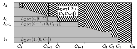
Figure 2: An illustration of dividing the schedule of OPT in the local analysis, i.e., dividing the (total size of) packets completed by OPT into $L_{\textsf{OPT\/}}(i,(0,C_{i}])$ and $L_{\textsf{OPT\/}}\left(\geq i,(C_{i},C_{i-1}]\right)$ for $i=1,\dots,k$. Rows correspond to packet sizes and the X-axis to time. Gray horizontal rectangles thus correspond to $L_{\textsf{OPT\/}}(i,(0,C_{i}])$, i.e., these rectangles represent the time interval $(0,C_{i}]$ and packets of size $\ell_{i}$ completed by OPT in $(0,C_{i}]$, whereas hatched rectangles correspond to $L_{\textsf{OPT\/}}\left(\geq i,(C_{i},C_{i-1}]\right)$.

The common scheme is the following. We carefully define a sequence of critical times $C_{k}\leq C_{k-1}\leq\cdots\leq C_{1}\leq C_{0}$, where $C_{0}=T$ is the end of the schedule, satisfying two properties: (1) till time $C_{i}$ the algorithm has completed almost all pending packets of size $\ell_{i}$ released before $C_{i}$ and (2) in $(C_{i},C_{i-1}]$, a packet of size $\ell_{i}$ is always pending. Properties (1) and (2) allow us to relate $L_{\textsf{OPT\/}}(i,(0,C_{i}])$ and $L_{\textsf{OPT\/}}(\geq i,(C_{i},C_{i-1}])$, respectively, to their “PG counterparts”. As each packet completed by OPT belongs to exactly one of these sets, summing the bounds gives the desired results; see Figure 2 for an illustration. These two facts together imply $R$-competitiveness of the algorithm for appropriate $R$ and speed $s$.

We first define the notion of $i$-good times so that they satisfy property (1), and then choose the critical times among their suprema so that those satisfy property (2) as well.

Definition 1.

Let $s\geq 1$ be the speedup. For $i=1,\ldots k$, time $t$ is called $i$-good if one of the following conditions holds:

1. At time $t$, algorithm ${\textsf{PG\/}(s)}$ starts a new phase by scheduling a packet of size larger than $\ell_{i}$, or

2. at time $t$, no packet of size $\ell_{i}$ is pending for ${\textsf{PG\/}(s)}$, or

3. $t=0$.

We define critical times $C_{0},C_{1},\ldots,C_{k}$ iteratively as follows:

• $C_{0}=T$, i.e., it is the end of the schedule.

• For $i=1,\ldots,k$, $C_{i}$ is the supremum of $i$-good times $t$ such that $t\leq C_{i-1}$.

Note that all $C_{i}$’s are defined and $C_{i}\geq 0$, as time $t=0$ is $i$-good for all $i$. The choice of $C_{i}$ implies that each $C_{i}$ is of one of the three types (the types are not disjoint):

• $C_{i}$ is $i$-good and a phase starts at $C_{i}$ (this includes $C_{i}=0$),

• $C_{i}$ is $i$-good and $C_{i}=C_{i-1}$, or

• there exists a packet of size $\ell_{i}$ pending at $C_{i}$, however, any such packet was released at $C_{i}$.

If the first two options do not apply, then the last one is the only remaining possibility (as otherwise some time in the non-empty interval $(C_{i},C_{i-1}]$ would be $i$-good); in this case, $C_{i}$ is not $i$-good, but only the supremum of $i$-good times.

First we bound the total size of packets of size $\ell_{i}$ completed before $C_{i}$; the proof actually only uses the fact that each $C_{i}$ is the supremum of $i$-good times and justifies the definition above.

Lemma 3.1.

Let $s\geq 1$ be the speedup. Then, for any $i$, it holds $L_{\textsf{OPT\/}}(i,(0,C_{i}])\leq L_{{\textsf{PG\/}(s)}}(i,(0,C_{i}])+\ell_{k}$.

Proof.

If $C_{i}$ is $i$-good and satisfies condition (i) in Definition 1, then by the description of Step (2) of the algorithm, the total size of pending packets of size $\ell_{i}$ is less than the size of the scheduled packet, which is at most $\ell_{k}$ and the lemma follows.

In all the remaining cases it holds that PG(s) has completed all the jobs of size $\ell_{i}$ released before $C_{i}$, thus the inequality holds trivially even without the additive term. ∎

Our remaining goal is to bound $L_{\textsf{OPT\/}}(\geq i,(C_{i},C_{i-1}])$. We divide $(C_{i},C_{i-1}]$ into $i$-segments by the faults. We prove the bounds separately for each $i$-segment. One important fact is that for the first $i$-segment we use only a loose bound, as we can use the additive constant. The critical part is then the bound for $i$-segments started by a fault, this part determines the competitive ratio and is different for each case. We summarize the general method by the following definition and master theorem.

Definition 2.

The interval $(u,v]$ is called the initial $i$-segment if $u=C_{i}$ and $v$ is either $C_{i-1}$ or the first time of a fault after $u$, whichever comes first.

The interval $(u,v]$ is called a proper $i$-segment if $u\in(C_{i},C_{i-1})$ is a time of a fault and $v$ is either $C_{i-1}$ or the first time of a fault after $u$, whichever comes first.

Note that there is no $i$-segment if $C_{i-1}=C_{i}$.

Theorem 3.2 (Master Theorem).

Let $s\geq 1$ be the speedup. Suppose that for $R\geq 1$ both of the following hold:

1. For each $i=1,\ldots,k$ and each proper $i$-segment $(u,v]$ with $v-u\geq\ell_{i}$, it holds that

   $$(R-1)L_{{\textsf{PG\/}(s)}}((u,v])+L_{{\textsf{PG\/}(s)}}(\geq i,(u,v])\;\geq\;L_{\textsf{OPT\/}}(\geq i,(u,v])\,.$$ (3.1)

2. For the initial $i$-segment $(u,v]$, it holds that

   $$L_{\textsf{PG\/}(s)}(\geq i,(u,v])\;>\;s(v-u)-4\ell_{k}\,.$$ (3.2)

Then ${\textsf{PG\/}(s)}$ is $R$-competitive.

Proof.

First note that for a proper $i$-segment $(u,v]$, $u$ is a fault time. Thus if $v-u<\ell_{i}$, then $L_{\textsf{OPT\/}}(\geq i,(u,v])=0$ and (3.1) is trivial. It follows that (3.1) holds even without the assumption $v-u\geq\ell_{i}$.

Now consider the initial $i$-segment $(u,v]$. We have $L_{\textsf{OPT\/}}(\geq i,(u,v])\leq\ell_{k}+v-u$, as at most a single packet started before $u$ can be completed. Combining this with (3.2) and using $s\geq 1$, we get $L_{\textsf{PG\/}(s)}(\geq i,(u,v])\;>\;s(v-u)-4\ell_{k}\;\geq\;v-u-4\ell_{k}\;\geq\;L_{\textsf{OPT\/}}(\geq i,(u,v])-5\ell_{k}$.

Summing this with (3.1) for all proper $i$-segments and using $R\geq 1$ we get

$$(R-1)L_{\textsf{PG\/}(s)}((C_{i},C_{i-1}])+L_{\textsf{PG\/}(s)}(\geq i,(C_{i},C_{i-1}])+5\ell_{k}$$

$$\geq L_{\textsf{OPT\/}}(\geq i,(C_{i},C_{i-1}])\,.$$ (3.3)

Note that for $C_{i}=C_{i-1}$, Equation (3.3) holds trivially.

To complete the proof, note that each completed job in the optimum contributes to exactly one among the $2k$ terms $L_{\textsf{OPT\/}}(\geq i,(C_{i},C_{i-1}])$ and $L_{\textsf{OPT\/}}(i,(0,C_{i}])$; similarly for $L_{\textsf{PG\/}(s)}$. Thus by summing both (3.3) and Lemma 3.1 for all $i=1,\ldots,k$ we obtain

$$L_{\textsf{OPT\/}} = \sum_{i=1}^{k}L_{\textsf{OPT\/}}\left(\geq i,(C_{i},C_{i-1}]\right)+\sum_{i=1}^{k}L_{\textsf{OPT\/}}(i,(0,C_{i}])$$

$$\leq \sum_{i=1}^{k}\bigg{(}(R-1)L_{\textsf{PG\/}(s)}((C_{i},C_{i-1}])+\left(L_{\textsf{PG\/}(s)}(\geq i,(C_{i},C_{i-1}])+5\ell_{k}\right)\bigg{)}$$

$$\mbox{}+\sum_{i=1}^{k}\left(L_{\textsf{PG\/}(s)}(i,(0,C_{i}])+\ell_{k}\right)$$

$$\leq (R-1)L_{\textsf{PG\/}(s)}+L_{\textsf{PG\/}(s)}+6k\ell_{k}\;=\;R\cdot L_{\textsf{PG\/}(s)}+6k\ell_{k}\,.$$

The theorem follows. ∎

3.2 Local Analysis of PrudentGreedy (PG)

The first part of the following lemma implies the condition (3.2) for the initial $i$-segments in all cases. The second part of the lemma is the base of the analysis of a proper $i$-segment, which is different in each situation.

Lemma 3.3.

1. If $(u,v]$ is the initial $i$-segment, then $L_{\textsf{PG\/}(s)}(\geq i,(u,v])>s(v-u)-4\ell_{k}$.

2. If $(u,v]$ is a proper $i$-segment and $v-u\geq\ell_{i}$ then $L_{\textsf{PG\/}(s)}((u,v])>s(v-u)/2$ and $L_{\textsf{PG\/}(s)}(\geq i,(u,v])>s(v-u)/2-\ell_{i}-\ell_{i-1}$. (Recall that $\ell_{0}=0$.)

Proof.

(i) If the phase that starts at $u$ or contains $u$ ends before $v$, let $u^{\prime}$ be its end; otherwise let $u^{\prime}=u$. We have $u^{\prime}\leq u+\ell_{i}/s$, as otherwise any packet of size $\ell_{i}$, pending throughout the $i$-segment by definition, would be an eligible choice in Step (3) of the algorithm, and the phase would not end before $v$. Using Lemma 2.2(ii), we have $L_{\textsf{PG\/}(s)}(<i,(u^{\prime},v])<\ell_{i}+\ell_{i-1}<2\ell_{k}$. Since at most one packet at the end of the segment is unfinished, we have $L_{\textsf{PG\/}(s)}(\geq i,(u,v])\geq L_{\textsf{PG\/}(s)}(\geq i,(u^{\prime},v])>s(v-u^{\prime})-3\ell_{k}\geq s(v-u)-4\ell_{k}$.

(ii) Let $(u,v]$ be a proper $i$-segment. Thus $u$ is a start of a phase that contains at least the whole interval $(u,v]$ by Lemma 2.2(ii). By the definition of $C_{i}$, $u$ is not $i$-good, so the phase starts by a packet of size at most $\ell_{i}$. If $v-u\geq\ell_{i}$ then the first packet finishes (as $s\geq 1$) and thus $L_{\textsf{PG\/}(s)}((u,v])>s(v-u)/2$ by Lemma 2.1. The total size of completed packets smaller than $\ell_{i}$ is less than $\ell_{i}+\ell_{i-1}$ by Lemma 2.2(ii), and thus $L_{\textsf{PG\/}(s)}(\geq i,(u,v])>s(v-u)/2-\ell_{i}-\ell_{i-1}$. ∎

3.2.1 General Packet Sizes

The next theorem gives a tradeoff of the competitive ratio of ${\textsf{PG\/}(s)}$ and the speedup $s$ using our local analysis. While Theorem 4.1 shows that ${\textsf{PG\/}(s)}$ is $1$-competitive for $s\geq 4$, here we give a weaker result that reflects the limits of the local analysis. However, for $s=1$ our local analysis is tight as already the lower bound from [1] shows that no algorithm is better than 3-competitive (for packet sizes $1$ and $2-\varepsilon$). See Figure 1 for an illustration of our upper and lower bounds on the competitive ratio of ${\textsf{PG\/}(s)}$.

Theorem 3.4.

${\textsf{PG\/}(s)}$ is $R_{s}$-competitive where:

$R_{s}=1+2/s$ for $s\in[1,4)$,

$R_{s}=2/3+2/s$ for $s\in[4,6)$, and

$R_{s}=1$ for $s\geq 6$.

Proof.

Lemma 3.3(i) implies the condition (3.2) for the initial $i$-segments. We now prove (3.1) for any proper $i$-segment $(u,v]$ with $v-u\geq\ell_{i}$ and appropriate $R$. The bound then follows by the Master Theorem.

Since there is a fault at time $u$, we have $L_{\textsf{OPT\/}}(\geq i,(u,v])\leq v-u$.

For $s\geq 6$, Lemma 3.3(ii) implies

$$L_{\textsf{PG\/}(s)}(\geq i,(u,v]) >s(v-u)/2-2\ell_{i}$$

$$\geq 3(v-u)-2(v-u)=v-u\geq L_{\textsf{OPT\/}}(\geq i,(u,v])\,,$$

which is (3.1) for $R=1$.

For $s\in[4,6)$, by Lemma 3.3(ii) we have $L_{\textsf{PG\/}(s)}((u,v])>s(v-u)/2$ and by multiplying it by $(2/s-1/3)$ we obtain

$$\left(\frac{2}{s}-\frac{1}{3}\right)\cdot L_{\textsf{PG\/}(s)}((u,v])>\left(1-\frac{s}{6}\right)(v-u)\,.$$

Thus to prove (3.1) for $R=2/3+2/s$, it suffices to show that

$$L_{\textsf{PG\/}(s)}(\geq i,(u,v])>\frac{s}{6}(v-u)\,,$$

as clearly $v-u\geq L_{\textsf{OPT\/}}(\geq i,(u,v])$. The remaining inequality again follows from Lemma 3.3(ii), but we need to consider two cases:

If $(v-u)\geq\frac{6}{s}\ell_{i}$, then

$$L_{\textsf{PG\/}(s)}(\geq i,(u,v])>\frac{s}{2}(v-u)-2\ell_{i}\geq\frac{s}{2}(v-u)-\frac{s}{3}(v-u)=\frac{s}{6}(v-u)\,.$$

On the other hand, if $(v-u)<\frac{6}{s}\ell_{i}$, then using $s\geq 4$ as well,

$$L_{\textsf{PG\/}(s)}(\geq i,(u,v])>\frac{s}{2}(v-u)-2\ell_{i}\geq 0\,,$$

therefore ${\textsf{PG\/}(s)}$ completes a packet of size at least $\ell_{i}$ which implies

$$L_{\textsf{PG\/}(s)}(\geq i,(u,v])\geq\ell_{i}>\frac{s}{6}(v-u)\,,$$

concluding the case of $s\in[4,6)$.

For $s\in[1,4)$, by Lemma 3.3(ii) we get $(2/s)\cdot L_{\textsf{PG\/}(s)}((u,v])>v-u\geq L_{\textsf{OPT\/}}(\geq i,(u,v])$, which implies (3.1) for $R=1+2/s$. ∎

3.2.2 Well-separated Packet Sizes

We can obtain better bounds on the speedup necessary for $1$-competitiveness if the packet sizes are sufficiently different. Namely, we call the packet sizes $\ell_{1},\ldots,\ell_{k}$ $\alpha$-separated if $\ell_{i}\geq\alpha\ell_{i-1}$ holds for $i=2,\ldots,k$.

Figure 3: A graph of $S_{\alpha}$ and the bounds on the speedup that we use in Theorem 3.5. Note that in the graph we also use Theorem 4.1 for $1$-competitiveness with speed $4$ (for any $\alpha$), but in the definition of $S_{\alpha}$ we do not take it into account.

Next, we show that for $\alpha$-separated packet sizes, $\textsf{PG\/}(S_{\alpha})$ is $1$-competitive for the following $S_{\alpha}$. We define

$$\alpha_{0} =\frac{1}{2}+\frac{1}{6}\sqrt{33}\approx 1.46\mbox{\,, which is the positive root of $3\alpha^{2}-3\alpha-2$.}$$

$$\alpha_{1} =\frac{3+\sqrt{17}}{4}\approx 1.78\mbox{\,, which is the positive root of $2\alpha^{2}-3\alpha-1$.}$$

$$S_{\alpha} =\begin{cases}\displaystyle\frac{4\alpha+2}{\alpha^{2}}&\mbox{ for $\alpha\in[1,\alpha_{0}]$,}\\[4.30554pt] 3+\frac{1}{\alpha}&\mbox{ for $\alpha\in[\alpha_{0},\alpha_{1})$, and}\\[4.30554pt] 2+\frac{2}{\alpha}&\mbox{ for $\alpha\geq\alpha_{1}$.}\end{cases}$$

See Figure 3 for a graph of $S_{\alpha}$ and all the bounds on it that we use. The value of $\alpha_{0}$ is chosen as the point where $(4\alpha+2)/\alpha^{2}=3+1/\alpha$. The value of $\alpha_{1}$ is chosen as the point from which the argument in case (viii) of the proof below works, which allows for a better result for $\alpha\geq\alpha_{1}$. If $s\geq S_{\alpha}$ then $s\geq(4\alpha+2)/\alpha^{2}$ and $s\geq 2+2/\alpha$ for all $\alpha$ and also $s\geq 3+1/\alpha$ for $\alpha<\alpha_{1}$; these facts follow from inspection of the functions and are useful for the analysis.

Note that $S_{\alpha}$ is decreasing in $\alpha$, with a single discontinuity at $\alpha_{1}$. We have $S_{1}=6$, matching the upper bound for 1-competitiveness using local analysis. We have $S_{2}=3$, i.e., $\textsf{PG\/}(3)$ is $1$-competitive for $2$-separated packet sizes, which includes the case of divisible packet sizes (however, only $s\geq 2.5$ is needed in the divisible case, as we show later). The limit of $S_{\alpha}$ for $\alpha\rightarrow+\infty$ is $2$. For $\alpha<(1+\sqrt{3})/2\approx 1.366$, we get $S_{\alpha}>4$, while Theorem 4.1 shows that ${\textsf{PG\/}(s)}$ is $1$-competitive for $s\geq 4$; the weaker result of Theorem 3.5 below reflect the limits of the local analysis.

Theorem 3.5.

Let $\alpha>1$. If the packet sizes are $\alpha$-separated, then ${\textsf{PG\/}(s)}$ is $1$-competitive for any $s\geq S_{\alpha}$.

Proof.

Lemma 3.3(i) implies (3.2). We now prove for any proper $i$-segment $(u,v]$ with $v-u\geq\ell_{i}$ that

$$L_{\textsf{PG\/}(s)}(\geq i,(u,v])\geq L_{\textsf{OPT\/}}(\geq i,(u,v])\,,$$ (3.4)

which is (3.1) for $R=1$. The bound then follows by the Master Theorem.

Let $X=L_{\textsf{OPT\/}}(\geq i,(u,v])$. Note that $X\leq v-u$.

Lemma 3.3(ii) together with $\ell_{i-1}\leq\ell_{i}/\alpha$ gives $L_{\textsf{PG\/}(s)}(\geq i,(u,v])>M$ for $M=sX/2-(1+1/\alpha)\ell_{i}$.

We use the fact that both $X$ and $L_{\textsf{PG\/}(s)}(\geq i,(u,v])$ are sums of some packet sizes $\ell_{j}$, $j\geq i$, and thus only some of the values are possible. However, the situation is quite complicated, as for example $\ell_{i+1}$, $\ell_{i+2}$, $2\ell_{i}$, $\ell_{i}+\ell_{i+1}$ are possible values, but their ordering may vary.

We distinguish several cases based on $X$ and $\alpha$. We note in advance that the first five cases suffice for $\alpha<\alpha_{1}$; only after completing the proof for $\alpha<\alpha_{1}$, we analyze the additional cases needed for $\alpha\geq\alpha_{1}$.

Case (i): $X=0$. Then (3.4) is trivial.

Case (ii): $X=\ell_{i}$. Using $s\geq 2+2/\alpha$, we obtain $M\geq(1+1/\alpha)\ell_{i}-(1+1/\alpha)\ell_{i}=0$. Thus $L_{\textsf{PG\/}(s)}(\geq i,(u,v])>M\geq 0$ which implies $L_{\textsf{PG\/}(s)}(\geq i,(u,v])\geq\ell_{i}=X$ and (3.4) holds.

Case (iii): $X=\ell_{i+1}$ and $\ell_{i+1}\leq 2\ell_{i}$. Using $s\geq(4\alpha+2)/\alpha^{2}$ and $X=\ell_{i+1}\geq\alpha\ell_{i}$, we obtain

$$M\geq\frac{s\ell_{i+1}}{2}-\left(1+\frac{1}{\alpha}\right)\ell_{i}\geq\left(2+\frac{1}{\alpha}\right)\ell_{i}-\left(1+\frac{1}{\alpha}\right)\ell_{i}=\ell_{i}\,.$$

Thus $L_{\textsf{PG\/}(s)}(\geq i,(u,v])>\ell_{i}$ which together with $\ell_{i+1}\leq 2\ell_{i}$ implies $L_{\textsf{PG\/}(s)}(\geq i,(u,v])\geq\ell_{i+1}=X$ and (3.4) holds.

Case (iv): $X\geq\alpha^{2}\ell_{i}$. (Note that this includes all cases when a packet of size at least $\ell_{i+2}$ contributes to $X$.) We first show that $s\geq 2(1+1/\alpha^{2}+1/\alpha^{3})$ by straightforward calculations with the golden ratio $\phi$:

• If $\alpha\leq\phi$, we have

  $$s\geq\frac{4\alpha+2}{\alpha^{2}}=2\left(\frac{2}{\alpha}+\frac{1}{\alpha^{2}}\right)\geq 2\left(1+\frac{1}{\alpha^{2}}+\frac{1}{\alpha^{3}}\right)\,,$$

  where we use $2/\alpha\geq 1+1/\alpha^{3}$ or equivalently $\alpha^{3}+1-2\alpha^{2}\leq 0$, which is true as

  $$\alpha^{3}+1-2\alpha^{2}=\alpha^{3}-\alpha^{2}+1-\alpha^{2}=\alpha^{2}(\alpha-1)-(\alpha+1)(\alpha-1)=(\alpha-1)(\alpha^{2}-\alpha-1)\leq 0\,,$$

  where the last inequality holds for $\alpha\in(1,\phi)$.

• If on the other hand $\alpha\geq\phi$, then $s\geq 2(1+1/\alpha)\geq 2(1+1/\alpha^{2}+1/\alpha^{3})$, as $1/\alpha\geq 1/\alpha^{2}+1/\alpha^{3}$ holds for $\alpha\geq\phi$.

Now we obtain

$$M-X \geq\left(\frac{s}{2}-1\right)X-\left(1+\frac{1}{\alpha}\right)\ell_{i}$$

$$\geq\left(1+\frac{1}{\alpha^{2}}+\frac{1}{\alpha^{3}}-1\right)X-\left(1+\frac{1}{\alpha}\right)\ell_{i}$$

$$\geq\left(\frac{1}{\alpha^{2}}+\frac{1}{\alpha^{3}}\right)\alpha^{2}\ell_{i}-\left(1+\frac{1}{\alpha}\right)\ell_{i}=0\enspace,$$

and (3.4) holds.

Case (v): $X\geq 2\ell_{i}$ and $\alpha<\alpha_{1}$. (Note that this includes all cases when at least two packets contribute to $X$, but we use it only if $\alpha<\alpha_{1}$.) Using $s\geq 3+1/\alpha$ we obtain

$$M-X\geq\left(\frac{1}{2}\left(3+\frac{1}{\alpha}\right)-1\right)X-\left(1+\frac{1}{\alpha}\right)\ell_{i}\geq\frac{1}{2}\left(1+\frac{1}{\alpha}\right)2\ell_{i}-\left(1+\frac{1}{\alpha}\right)\ell_{i}=0\enspace,$$

and (3.4) holds.

Proof for $\alpha<\alpha_{1}$: We now observe that for $\alpha<\alpha_{1}$, we have exhausted all the possible values of $X$. Indeed, if (v) does not apply, then at most a single packet contributes to $X$, and one of the cases (i)-(iv) applies, as (iv) covers the case when $X\geq\ell_{i+2}$, and as $X=\ell_{i+1}$ is covered by (iii) or (v). Thus (3.4) holds and the proof is complete.

Proof for $\alpha\geq\alpha_{1}$: We now analyze the remaining cases for $\alpha\geq\alpha_{1}$.

Case (vi): $X\geq(\alpha+1)\ell_{i}$. (Note that this includes all cases when two packets not both of size $\ell_{i}$ contribute to $X$.) Using $s\geq 2+2/\alpha$ we obtain

$$M-X\geq\left(1+\frac{1}{\alpha}-1\right)X-\left(1+\frac{1}{\alpha}\right)\ell_{i}\geq\frac{1}{\alpha}(\alpha+1)\ell_{i}-\left(1+\frac{1}{\alpha}\right)\ell_{i}=0$$

and (3.4) holds.

Case (vii): $X=n\cdot\ell_{i}<(\alpha+1)\ell_{i}$ for some $n=2,3,\ldots$. Since $\alpha>\alpha_{1}>\phi$, we have $\ell_{i+1}>\ell_{i}+\ell_{i-1}$. This implies that the first packet of size at least $\ell_{i}$ that is scheduled in the phase has size equal to $\ell_{i}$ by the condition in Step (3) of the algorithm. Thus, if also a packet of size larger than $\ell_{i}$ contributes to $L_{\textsf{PG\/}(s)}(\geq i,(u,v])$, we have

$$L_{\textsf{PG\/}(s)}(\geq i,(u,v])\geq\ell_{i+1}+\ell_{i}\geq(\alpha+1)\ell_{i}>X$$

by the case condition and (3.4) holds. Otherwise $L_{\textsf{PG\/}(s)}(\geq i,(u,v])$ is a multiple of $\ell_{i}$. Using $s\geq 2+2/\alpha$, we obtain

$$M\geq\left(1+\frac{1}{\alpha}\right)n\cdot\ell_{i}-\left(1+\frac{1}{\alpha}\right)\ell_{i}\geq(n-1)\left(1+\frac{1}{\alpha}\right)\ell_{i}>(n-1)\ell_{i}\,.$$

This, together with divisibility by $\ell_{i}$ implies $L_{\textsf{PG\/}(s)}(\geq i,(u,v])\geq n\cdot\ell_{i}=X$ and (3.4) holds again.

Case (viii): $X=\ell_{i+1}$ and $\ell_{i+1}>2\ell_{i}$. We distinguish two subcases depending on the size of the unfinished packet of PG(s) in this phase.

If the unfinished packet has size at most $\ell_{i+1}$, the size of the completed packets is bounded by

$$L_{\textsf{PG\/}(s)}((u,v])>sX-\ell_{i+1}=(s-1)\ell_{i+1}\geq\left(1+\frac{2}{\alpha}\right)\ell_{i+1}\,,$$

using $s\geq 2+2/\alpha$. Since the total size of packets smaller than $\ell_{i}$ is less then $(1+1/\alpha)\ell_{i}$ by Lemma 2.2(ii), we obtain

$$L_{\textsf{PG\/}(s)}(\geq i,(u,v])-X>\frac{2\ell_{i+1}}{\alpha}-\left(1+\frac{1}{\alpha}\right)\ell_{i}\geq 2\ell_{i}-\left(1+\frac{1}{\alpha}\right)\ell_{i}>0\,,$$

where the penultimate inequality uses $\ell_{i+1}/\alpha\geq\ell_{i}$. Thus (3.4) holds.

Otherwise the unfinished packet has size at least $\ell_{i+2}$ and, by Step (3) of the algorithm, also $L_{\textsf{PG\/}(s)}((u,v])>\ell_{i+2}$. We have $\ell_{i+2}\geq\alpha\ell_{i+1}$ and by the case condition $\ell_{i+1}>2\ell_{i}$ we obtain

$$L_{\textsf{PG\/}(s)}(\geq i,(u,v])-X>(\alpha-1)\ell_{i+1}-\left(1+\frac{1}{\alpha}\right)\ell_{i}>2(\alpha-1)\ell_{i}-\left(1+\frac{1}{\alpha}\right)\ell_{i}\geq 0\,,$$

as the definition of $\alpha_{1}$ implies that $2(\alpha-1)\geq 1+1/\alpha$ for $\alpha\geq\alpha_{1}$. Thus (3.4) holds.

We now observe that we have exhausted all the possible values of $X$ for $\alpha\geq\alpha_{1}$. Indeed, if at least two packets contribute to $X$, either (vi) or (vii) applies. Otherwise, at most a single packet contributes to $X$, and one of the cases (i)-(iv) or (viii) applies, as (iv) covers the case when $X\geq\ell_{i+2}$. Thus (3.4) holds and the proof is complete. ∎

3.2.3 Divisible Packet Sizes

Now, we turn briefly to even more restricted divisible instances considered by Jurdziński et al. [10], which are a special case of $2$-separated instances. Namely, we improve upon Theorem 3.5 in Theorem 3.6 presented below in the following sense: While the former guarantees that PG(s) is $1$-competitive on (more general) $2$-separated instances at speed $s\geq 3$, the latter shows that speed $s\geq 2.5$ is sufficient for (more restricted) divisible instances. Moreover, we note that that by an example in Section 3.3, the bound of Theorem 3.6 is tight, i.e., PG(s) is not $1$-competitive for $s<2.5$, even on divisible instances.

Theorem 3.6.

If the packet sizes are divisible, then ${\textsf{PG\/}(s)}$ is 1-competitive for $s\geq 2.5$.

Proof.

Lemma 3.3(i) implies (3.2). We now prove (3.1) for any proper $i$-segment $(u,v]$ with $v-u\geq\ell_{i}$ and $R=1$. The bound then follows by the Master Theorem. Since there is a fault at time $u$, we have $L_{\textsf{OPT\/}}(\geq i,(u,v])\leq v-u$.

By divisibility we have $L_{\textsf{OPT\/}}(\geq i,(u,v])=n\ell_{i}$ for some nonnegative integer $n$. We distinguish two cases based on the size of the last packet started by PG in the $i$-segment $(u,v]$, which is possibly unfinished due to a fault at $v$.

If the unfinished packet has size at most $n\ell_{i}$, then

$$L_{\textsf{PG\/}(s)}(\geq i,(u,v])>5(v-u)/2-\ell_{i}-\ell_{i-1}-n\ell_{i}\geq 5n\ell_{i}/2-3\ell_{i}/2-n\ell_{i}\geq(n-1)\ell_{i}$$

by Lemma 2.1 and Lemma 2.2(ii). Divisibility now implies $L_{\textsf{PG\/}(s)}(\geq i,(u,v])\geq n\ell_{i}=L_{\textsf{OPT\/}}(\geq i,(u,v])$.

Otherwise, by divisibility the size of the unfinished packet is at least $(n+1)\ell_{i}$ and the size of the completed packets is larger by the condition in Step (3) of the algorithm; here we also use the fact that ${\textsf{PG\/}(s)}$ completes the packet started at $u$, as its size is at most $\ell_{i}\leq v-u$ (otherwise, $u$ would be $i$-good, thus $C_{i}\geq u$ and $(u,v]$ is not a proper $i$-segment). Thus $L_{\textsf{PG\/}(s)}(\geq i,(u,v])>(n+1)\ell_{i}-3\ell_{i}/2\geq(n-1/2)\ell_{i}$. Divisibility again implies $L_{\textsf{PG\/}(s)}(\geq i,(u,v])\geq n\ell_{i}=L_{\textsf{OPT\/}}(\geq i,(u,v])$, which shows (3.1). ∎

3.3 Some Examples for PG

3.3.1 General Packet Sizes

Speeds below 2

We show an instance on which the performance of PG(s) matches the bound of Theorem 3.4.

Remark.

PG(s) has competitive ratio at least $1+2/s$ for $s<2$.

Proof.

Choose a large enough integer $N$. At time 0 the following packets are released: $2N$ packets of size $1$, one packet of size $2$ and $N$ packet of size $4/s-\varepsilon$ for a small enough $\varepsilon>0$ such that it holds $2<4/s-\varepsilon$. These are all packets in the instance.

First there are $N$ phases, each of length $4/s-\varepsilon$ and ending by a fault. OPT completes a packet of size $4/s-\varepsilon$ in each phase, while PG(s) completes $2$ packets of size $1$ and then it starts a packet of size $2$ which is not finished.

Then there is a fault every $1$ unit of time, so that OPT completes all packets of size 1, while the algorithm has no pending packet of size 1 and as $s<2$ the length of the phase is not sufficient to finish a longer packet.

Overall, OPT completes packets of total size $2+4/s-\varepsilon$ per phase, while the algorithm completes packets of total size only $2$ per phase. The ratio thus tends to $1+2/s$ as $\varepsilon\rightarrow 0$. ∎

Speeds between 2 and 4

Now we show an instance which proves that PG(s) is not $1$-competitive for $s<4$. In particular, this implies that the speed sufficient for $1$-competitiveness in Theorem 4.1, which we prove later, cannot be improved.

Remark.

PG(s) has competitive ratio at least $4/s>1$ for $s\in[2,4)$.

Proof.

Choose a large enough integer $y$. There will be four packet sizes: $1,x,y$ and $z$ such that $1<x<y<z$, $z=x+y-1$, and $x=y\cdot(s-2)/2+2$; as $s\geq 2$ it holds $x>1$ and as $s<4$ we have $x\leq y-1$ for a large enough $y$.

We will have $N$ phases again. At time 0 the adversary releases all $N(y-1)$ packets of size $1$, all $N$ packets of size $y$ and a single packet of size $z$ (never completed by either OPT or PG(s)), whereas the packets of size $x$ are released one per phase.

In each phase PG(s) completes, in this order: $y-1$ packets of size $1$ and then a packet of size $x$, which has arrived just after the $y-1$ packets of size $1$ are completed. Next, it will start a packet of size $z$ and fail due to a jam. We show that OPT will complete a packet of size $y$. To this end, it is required that $y<2(x+y-1)/s$, or equivalently $x>y\cdot(s-2)/2+1$ which holds by the choice of $x$.

After these $N$ phases, we will have jams every $1$ unit of time, so that OPT can complete all the $N(y-1)$ packets of size $1$, while PG(s) will be unable to complete any packet (of size $y$ or larger). The ratio per phase is

$$\frac{\textsf{OPT\/}}{{\textsf{PG\/}(s)}}=\frac{y-1+y}{y-1+x}=\frac{2y-1}{y-1+\frac{y\cdot(s-2)}{2}+2}=\frac{2y-1}{\frac{y\cdot s}{2}+1}$$

which tends to $4/s$ as $y\to\infty$.

∎

This example also disproves the claim of Anta et al. [2] that their $(m,\beta)$-LAF algorithm is $1$-competitive at speed $3.5$, even for one channel, i.e., $m=1$, where it behaves almost exactly as PG(s) — the sole difference is that LAF starts a phase by choosing a “random” packet. As this algorithm is deterministic, we understand this to mean “arbitrary”, so in particular the same as chosen by PG(s).

3.3.2 Divisible Case

We give an example that shows that PG is not very good for divisible instances, in particular it is not $1$-competitive for any speed $s<2.5$ and thus the bound in Theorem 3.6 is tight.

Remark.

PG(s) has competitive ratio at least $4/3$ on divisible instances if $s<2.5$.

Proof.

We use packets of sizes $1$, $\ell$, and $2\ell$ and we take $\ell$ sufficiently large compared to the given speed or competitive ratio. There are many packets of size $1$ and $2\ell$ available at the beginning, the packets of size $\ell$ arrive at specific times where PG schedules them immediately.

The faults occur at times divisible by $2\ell$, so the optimum schedules one packet of size $2\ell$ in each phase between two faults. We have $N$ such phases, $N(2\ell-1)$ packets of size $1$ and $N$ packets of size $2\ell$ available at the beginning. In each phase, ${\textsf{PG\/}(s)}$ schedules $2\ell-1$ packets of size $1$, then a packet of size $\ell$ arrives and is scheduled, and then a packet of size $2\ell$ is scheduled. The algorithm would need speed $2.5-1/(2\ell)$ to complete it. So, for $\ell$ large, the algorithm completes only packets of total size $3\ell-1$ per phase. After these $N$ phases, we have faults every 1 unit of time, so the optimum schedules all packets of size $1$, but the algorithm has no packet of size 1 pending and it is unable to finish a longer packet. The optimum thus finishes all packets $2\ell$ plus all small packets, a total of $4\ell-1$ per phase. Thus the ratio tends to $4/3$ as $\ell\to\infty$.

∎

3.4 Algorithm PG-DIV and its Analysis

We introduce our other algorithm PG-DIV designed for divisible instances. Actually, it is rather a fine-tuned version of PG, as it differs from it only in Step (3), where PG-DIV enforces an additional divisibility condition, set apart by italics in its formalization below. Then, using our framework of local analysis from this section, we give a simple proof that PG-DIV matches the performance of the algorithms from [10] on divisible instances.

Algorithm PG-DIV (1) If no packet is pending, stay idle until the next release time. (2) Let $i$ be the maximal $i\leq k$ such that there is a pending packet of size $\ell_{i}$ and $\ell(P^{<i})<\ell_{i}$. Schedule a packet of size $\ell_{i}$ and set $t_{B}=t$. (3) Choose the maximum $i$ such that
 (i) there is a pending packet of size $\ell_{i}$,
 (ii) $\ell_{i}\leq{\mbox{rel}}(t)$ and
 (iii) $\ell_{i}$ divides ${\mbox{rel}}(t)$.
Schedule a packet of size $\ell_{i}$. Repeat Step (3) as long as such $i$ exists. (4) If no packet satisfies the condition in Step (3), go to Step (1).

Throughout the section we assume that the packet sizes are divisible. We note that Lemmata 2.1 and 3.1 and the Master Theorem apply to PG-DIV as well, since their proofs are not influenced by the divisibility condition. In particular, the definition of critical times $C_{i}$ (Definition 1) remains the same. Thus, this section is devoted to leveraging divisibility to prove stronger stronger analogues of Lemma 2.2 and Lemma 3.3 (which are not needed to prove the Master Theorem) in this order. Once established, these are combined with the Master Theorem to prove that $\textsf{PG-DIV\/}(2)$ is $1$-competitive and $\textsf{PG-DIV\/}(1)$ is $2$-competitive. Recall that ${\mbox{rel}}(t)=s\cdot(t-t_{B})$ is the relative time after the start of the current phase $t_{B}$, scaled by the speed of the algorithm.

Lemma 3.7.

1. If PG-DIV starts or completes a packet of size $\ell_{i}$ at time $t$, then $\ell_{i}$ divides ${\mbox{rel}}(t)$.

2. Let $t$ be a time with ${\mbox{rel}}(t)$ divisible by $\ell_{i}$ and ${\mbox{rel}}(t)>0$. If a packet of size $\ell_{i}$ is pending at time $t$, then PG-DIV starts or continues running a packet of size at least $\ell_{i}$ at time $t$.

3. If at the beginning of phase at time $u$ a packet of size $\ell_{i}$ is pending and no fault occurs before time $t=u+\ell_{i}/s$, then the phase does not end before $t$.

Proof.

(i) follows trivially from the description of the algorithm.

(ii): If PG-DIV continues running some packet at $t$, it cannot be a packet smaller than $\ell_{i}$ by (i) and the claim follows. If PG-DIV  starts a new packet, then a packet of size $\ell_{i}$ is pending by the assumption. Furthermore, it satisfies all the conditions from Step 3 of the algorithm, as ${\mbox{rel}}(t)$ is divisible by $\ell_{i}$ and ${\mbox{rel}}(t)\geq\ell_{i}$ (from ${\mbox{rel}}(t)>0$ and divisibility). Thus the algorithm starts a packet of size at least $\ell_{i}$.

(iii): We proceed by induction on $i$. Assume that no fault happens before $t$. If the phase starts by a packet of size at least $\ell_{i}$, the claim holds trivially, as the packet is not completed before $t$. This also proves the base of the induction for $i=1$.

It remains to handle the case when the phase starts by a packet smaller than $\ell_{i}$. Let $P^{<i}$ be the set of all packets of size smaller than $\ell_{i}$ pending at time $u$. By the Step (2) of the algorithm, $\ell(P^{<i})\geq\ell_{i}$. We show that all packets of $P^{<i}$ are completed if no fault happens, which implies that the phase does not end before $t$.

Let $j$ be such that $\ell_{j}$ is the maximum size of a packet in $P^{<i}$; note that $j$ exists, as the phase starts by a packet smaller than $\ell_{i}$. By the induction assumption, the phase does not end before time $t^{\prime}=u+\ell_{j}/s$. From time $t^{\prime}$ on, the conditions in Step (3) guarantee that the remaining packets from $P^{<i}$ are processed from the largest ones, possibly interleaved with some of the newly arriving packets of larger sizes, as ${\mbox{rel}}(\tau)$ for the current time $\tau\geq t^{\prime}$ such that a packet completes at $\tau$ is always divisible by the size of the largest pending packet from $P^{<i}$. This shows that the phase cannot end before all packets from $P^{<i}$ are completed if no fault happens. ∎

Now we prove a stronger analogue of Lemma 3.3.

Lemma 3.8.

1. If $(u,v]$ is the initial $i$-segment, then

   $$L_{\textsf{PG-DIV\/}(s)}(\geq i,(u,v])>s(v-u)-3\ell_{k}\,.$$

2. If $(u,v]$ is a proper $i$-segment and $v-u\geq\ell_{i}$ then

   $$L_{\textsf{PG-DIV\/}(s)}(\geq i,(u,v])>s(v-u)/2-\ell_{i}\,.$$

   Furthermore, $L_{\textsf{PG-DIV\/}(s)}((u,v])>s(v-u)/2$ and $L_{\textsf{PG-DIV\/}(s)}((u,v])$ is divisible by $\ell_{i}$.

Proof.

Suppose that time $t\in[u,v)$ satisfies that ${\mbox{rel}}(t)$ is divisible by $\ell_{i}$ and ${\mbox{rel}}(t)>0$. Then observe that Lemma 3.7(ii) together with the assumption that a packet of size $\ell_{i}$ is always pending in $[u,v)$ implies that from time $t$ on only packets of size at least $\ell_{i}$ are scheduled, and thus the current phase does not end before $v$.

For a proper $i$-segment $(u,v]$, the previous observation for $t=u+\ell_{i}/s$ immediately implies (ii): Observe that $t\leq v$ by the assumption of (ii). Now $L_{\textsf{PG-DIV\/}(s)}(<i,(u,v])$ is either equal to $0$ (if the phase starts by a packet of size $\ell_{i}$ at time $u$), or equal to $\ell_{i}$ (if the phase starts by a smaller packet). In both cases $\ell_{i}$ divides $L_{\textsf{PG-DIV\/}(s)}(<i,(u,v])$ and thus also $L_{\textsf{PG-DIV\/}(s)}((u,v])$. As in the analysis of PG, the total size of completed packets is more than $s(v-u)/2$ and (ii) follows.

For the initial $i$-segment $(u,v]$ we first observe that the claim is trivial if $s(v-u)\leq 2\ell_{i}$. So we may assume that $u+2\ell_{i}/s\leq v$. Now we distinguish two cases:

1. The phase of $u$ ends at some time $u^{\prime}\leq u+\ell_{i}/s$: Then, by Lemma 3.7(iii) and the initial observation, the phase that immediately follows the one of $u$ does not end in $(u^{\prime},v)$ and from time $u^{\prime}+\ell_{i}/s$ on, only packets of size at least $\ell_{i}$ are scheduled. Thus $L_{\textsf{PG-DIV\/}(s)}(<i,(u,v])\leq 2\ell_{i}$.

2. The phase of $u$ does not end by time $u+\ell_{i}/s$: Thus there exists $t\in(u,u+\ell_{i}/s]$ such that $\ell_{i}$ divides ${\mbox{rel}}(t)$ and also ${\mbox{rel}}(t)>0$ as $t>u$. Using the initial observation for this $t$ we obtain that the phase does not end in $(u,v)$ and from time $t$ on only packets of size at least $\ell_{i}$ are scheduled. Thus $L_{\textsf{PG-DIV\/}(s)}(<i,(u,v])\leq\ell_{i}$.

In both cases $L_{\textsf{PG-DIV\/}(s)}(<i,(u,v])\leq 2\ell_{i}$, furthermore only a single packet is possibly unfinished at time $v$. Thus $L_{\textsf{PG-DIV\/}(s)}(\geq i,(u,v])>s(v-u)-2\ell_{i}-\ell_{k}$ and (i) follows. ∎

Theorem 3.9.

Let the packet sizes be divisible. Then $\textsf{PG-DIV\/}(1)$ is $2$-competitive. Also, for any speed $s\geq 2$, ${\textsf{PG-DIV\/}(s)}$ is $1$-competitive.

Proof.

Lemma 3.8(i) implies (3.2). We now prove (3.1) for any proper $i$-segment $(u,v]$ with $v-u\geq\ell_{i}$ and appropriate $R$. The theorem then follows by the Master Theorem.

Since $u$ is a time of a fault, we have $L_{\textsf{OPT\/}}(\geq i,(u,v])\leq v-u$. If $L_{\textsf{OPT\/}}(\geq i,(u,v])=0$, (3.1) is trivial. Otherwise $L_{\textsf{OPT\/}}(\geq i,(u,v])\geq\ell_{i}$, thus $v-u\geq\ell_{i}$ and the assumption of Lemma 3.8(ii) holds.

For $s\geq 2$, Lemma 3.8(ii) implies

$$L_{\textsf{PG-DIV\/}(s)}(\geq i,(u,v])>s(v-u)/2-\ell_{i}\geq v-u-\ell_{i}\geq L_{\textsf{OPT\/}}(\geq i,(u,v])-\ell_{i}\,.$$

Since both $L_{\textsf{PG-DIV\/}(s)}(\geq i,(u,v])$ and $L_{\textsf{OPT\/}}(\geq i,(u,v])$ are divisible by $\ell_{i}$, this implies $L_{\textsf{PG-DIV\/}(s)}(\geq i,(u,v])\geq L_{\textsf{OPT\/}}(\geq i,(u,v])$, i.e., (3.1) holds for $R=1$.

For $s=1$, Lemma 3.8(ii) implies

$$L_{\textsf{PG-DIV\/}}((u,v])+L_{\textsf{PG-DIV\/}}(\geq i,(u,v]) >(v-u)/2+(v-u)/2-\ell_{i}$$

$$\geq v-u-\ell_{i}\geq L_{\textsf{OPT\/}}(\geq i,(u,v])-\ell_{i}\,.$$

Since $L_{\textsf{PG-DIV\/}}((u,v])$, $L_{\textsf{PG-DIV\/}}(\geq i,(u,v])$, and $L_{\textsf{OPT\/}}(\geq i,(u,v])$ are all divisible by $\ell_{i}$, this implies $L_{\textsf{PG-DIV\/}}((u,v])+L_{\textsf{PG-DIV\/}}(\geq i,(u,v])\geq L_{\textsf{OPT\/}}(\geq i,(u,v])$, i.e., (3.1) holds for $R=2$. ∎

3.4.1 Example with Two Divisible Packet Sizes

We show that for our algorithms speed $2$ is necessary if we want a ratio below $2$, even if there are only two packet sizes in the instance. This matches the upper bound given in Theorem 3.4 for $\textsf{PG\/}(2)$ and our upper bounds for $\textsf{PG-DIV\/}(s)$ on divisible instances, i.e., ratio $2$ for $s<2$ and ratio $1$ for $s\geq 2$. We remark that by Theorem 5.1, no deterministic algorithm can be $1$-competitive with speed $s<2$ on divisible instances, but this example shows a stronger lower bound for our algorithms, namely that their ratios are at least $2$.

Remark.

PG and PG-DIV have ratio no smaller than $2$ when $s<2$, even if packet sizes are only $1$ and $\ell\geq\max\{s+\epsilon,\ \epsilon/(2-s)\}$ for an arbitrarily small $\epsilon>0$.

Proof.

We denote either algorithm by ALG. There will be $N$ phases, that all look the same: In each phase, issue one packet of size $\ell$ and $\ell$ packets of size 1, and have the phase end by a fault at time $(2\ell-\varepsilon)/s\geq\ell$ which holds by the bounds on $\ell$. Then ALG will complete all $\ell$ packets of size $1$ but will not complete the one of size $\ell$. By the previous inequality, OPT can complete the packet of size $\ell$ within the phase. Once all $N$ phases are over, the jams occur every $1$ unit of time, which allows OPT completing all $N\ell$ remaining packets of size $1$. However, ALG is unable to complete any of the packets of size $\ell$. Thus the ratio is $2$. ∎

4 PrudentGreedy with Speed 4

In this section we prove that speed 4 is sufficient for PG to be 1-competitive. An example in Section 3.3 show that speed 4 is also necessary for our algorithm.

Theorem 4.1.

${\textsf{PG\/}(s)}$ is 1-competitive for $s\geq 4$.

Intuition

For $s\geq 4$ we have that if at the start of a phase ${\textsf{PG\/}(s)}$ has a packet of size $\ell_{i}$ pending and the phase has length at least $\ell_{i}$, then ${\textsf{PG\/}(s)}$ completes a packet of size at least $\ell_{i}$. To show this, assume that the phase starts at time $t$. Then the first packet $p$ of size at least $\ell_{i}$ is started before time $t+2\ell_{i}/s$ by Lemma 2.2(ii) and by the condition in Step (3) it has size smaller than $2\ell_{i}$. Thus it completes before time $t+4\ell_{i}/s\leq t+\ell_{i}$, which is before the end of the phase. This property does not hold for $s<4$. It is important in our proof, as it shows that if the optimal schedule completes a job of some size, and such job is pending for ${\textsf{PG\/}(s)}$, then ${\textsf{PG\/}(s)}$ completes a job of the same size or larger. However, this is not sufficient to complete the proof by a local (phase-by-phase) analysis similar to the previous section, as the next example shows.

Assume that at the beginning, we release $N$ packets of size $1$, $N$ packets of size $1.5-2\varepsilon$, one packet of size $3-2\varepsilon$ and a sufficient number of packets of size $1-\varepsilon$, for a small $\varepsilon>0$. Our focus is on packets of size at least $1$. Supposing $s=4$ we have the following phases:

• First, there are $N$ phases of length $1$. In each phase the optimum completes a packet of size $1$, while among packets of size at least $1$, ${\textsf{PG\/}(s)}$ completes a packet of size $1.5-2\varepsilon$, as it starts packets of sizes $1-\varepsilon$, $1-\varepsilon$, $1.5-2\varepsilon$, $3-2\varepsilon$, in this order, and the last packet is jammed.

• Then there are $N$ phases of length $1.5-2\varepsilon$ where the optimum completes a packet of size $1.5-2\varepsilon$ while among packets of size at least $1$, the algorithm completes only a single packet of size $1$, as it starts packets of sizes $1-\varepsilon$, $1-\varepsilon$, $1$, $3-2\varepsilon$, in this order. The last packet is jammed, since for $s=4$ the phase must have length at least $1.5-\varepsilon$ to complete it.

In phases of the second type, the algorithm does not complete more (in terms of total size) packets of size at least $1$ than the optimum. Nevertheless, in our example, packets of size $1.5-2\varepsilon$ were already finished by the algorithm, and this is a general rule. The novelty in our proof is a complex charging argument that exploits such subtle interaction between phases.

Outline of the proof

We define critical times $C^{\prime}_{i}$ similarly as before, but without the condition that they should be ordered (thus either $C^{\prime}_{i}\leq C^{\prime}_{i-1}$ or $C^{\prime}_{i}>C^{\prime}_{i-1}$ may hold). Then, since the algorithm has nearly no pending packets of size $\ell_{i}$ just before $C^{\prime}_{i}$, we can charge almost all adversary’s packets of size $\ell_{i}$ started before $C^{\prime}_{i}$ to algorithm’s packets of size $\ell_{i}$ completed before $C^{\prime}_{i}$ in a 1-to-1 fashion; we thus call these charges 1-to-1 charges. We account for the first few packets of each size completed at the beginning of ADV, the schedule of the adversary, in the additive constant of the competitive ratio, thereby shifting the targets of the 1-to-1 charges backward in time. This also resolves what to do with the yet uncharged packets pending for the algorithm just before $C^{\prime}_{i}$.

After the critical time $C^{\prime}_{i}$, packets of size $\ell_{i}$ are always pending for the algorithm, and thus (as we observed above) the algorithm schedules a packet of size at least $\ell_{i}$ when the adversary completes a packet of size $\ell_{i}$. It is actually more convenient not to work with phases, but partition the schedule into blocks inbetween successive faults. A block can contain several phases of the algorithm separated by an execution of Step (4); however, in the most important and tight part of the analysis the blocks coincide with phases.

In the crucial lemma of the proof, based on these observations and their refinements, we show that we can assign the remaining packets in ADV to algorithm’s packets in the same block so that for each algorithm’s packet $q$ the total size of packets assigned to it is at most $\ell(q)$. However, we cannot use this assignment directly to charge the remaining packets, as some of the algorithm’s big packets may receive 1-to-1 charges, and in this case the analysis needs to handle the interaction of different blocks. This very issue can be seen even in our introductory example.

To deal with this, we process blocks in the order of time from the beginning to the end of the schedule, simultaneously completing the charging to the packets in the current block of the schedule of PG(s) and possibly modifying ADV in the future blocks. In fact, in the assignment described above, we include not only the packets in ADV without 1-to-1 charges, but also packets in ADV with a 1-to-1 charge to a later block. After creating the assignment, if we have a packet $q$ in PG that receives a 1-to-1 charge from a packet $p$ in a later block of ADV, we remove $p$ from ADV in that later block and replace it there by the packets assigned to $q$ (that are guaranteed to be of smaller total size than $p$). After these swaps, the 1-to-1 charges together with the assignment form a valid charging that charges the remaining not swapped packets in ADV in this block together with the removed packets from the later blocks in ADV to the packets of PG(s) in the current block. This charging is now independent of the other blocks, so we can continue with the next block.

4.1 Blocks, Critical Times, 1-to-1 Charges and the Additive Constant

We now formally define the notions of blocks and (modified) critical times.

Definition 3.

Let $f_{1},f_{2},\ldots,f_{N}$ be the times of faults. Let $f_{0}=0$ and $f_{N+1}=T$ is the end of schedule. Then the time interval $(f_{i},f_{i+1}]$, $i=0,\ldots,N$, is called a block.

Definition 4.

For $i=1,\ldots k$, the critical time $C^{\prime}_{i}$ is the supremum of $i$-good times $t\in[0,T]$, where $T$ is the end of the schedule and $i$-good times are as defined in Definition 1.

All $C^{\prime}_{i}$’s are defined, as $t=0$ is $i$-good for all $i$. Similarly to Section 3.1, each $C^{\prime}_{i}$ is of one of the following types: (i) $C^{\prime}_{i}$ starts a phase and a packet larger than $\ell_{i}$ is scheduled, (ii) $C^{\prime}_{i}=0$, (iii) $C^{\prime}_{i}=T$, or (iv) just before time $C^{\prime}_{i}$ no packet of size $\ell_{i}$ is pending but at time $C^{\prime}_{i}$ one or more packets of size $\ell_{i}$ are pending; in this case $C^{\prime}_{i}$ is not $i$-good but only the supremum of $i$-good times. We observe that in each case, at time $C^{\prime}_{i}$ the total size of packets $p$ of size $\ell_{i}$ pending for ${\textsf{PG\/}(s)}$ and released before $C^{\prime}_{i}$ is less than $\ell_{k}$.

Next we define the set of packets that contribute to the additive constant.

Definition 5.

Let the set $A$ contain for each $i=1,\dots,k$:

1. the first $\lceil 4\ell_{k}/\ell_{i}\rceil$ packets of size $\ell_{i}$ completed by the adversary, and

2. the first $\lceil 4\ell_{k}/\ell_{i}\rceil$ packets of size $\ell_{i}$ completed by the adversary after $C^{\prime}_{i}$.

If there are not sufficiently many packets of size $\ell_{i}$ completed by the adversary in (i) or (ii), we take all the packets in (i) or all the packets completed after $C^{\prime}_{i}$ in (ii), respectively.

For each $i$, we put into $A$ packets of size $\ell_{i}$ of total size at most $10\ell_{k}$. Thus we have $\ell(A)=\mathcal{O}(k\ell_{k})$ which implies that packets in $A$ can be counted in the additive constant.

We define 1-to-1 charges for packets of size $\ell_{i}$ as follows. Let $p_{1}$, $p_{2}$, …, $p_{n}$ be all the packets of size $\ell_{i}$ started by the adversary before $C^{\prime}_{i}$ that are not in $A$. We claim that ${\textsf{PG\/}(s)}$ completes at least $n$ packets of size $\ell_{i}$ before $C^{\prime}_{i}$ if $n\geq 1$. Indeed, if $n\geq 1$, before time $C^{\prime}_{i}$ at least $n+\lceil 4\ell_{k}/\ell_{i}\rceil$ packets of size $\ell_{i}$ are started by the adversary and thus released; by the definition of $C^{\prime}_{i}$ at time $C^{\prime}_{i}$ fewer than $\ell_{k}/\ell_{i}$ of them are pending for ${\textsf{PG\/}(s)}$, one may be running and the remaining ones must be completed. We now charge each $p_{m}$ to the $m$th packet of size $\ell_{i}$ completed by ${\textsf{PG\/}(s)}$. Note that each packet started by the adversary is charged at most once and each packet completed by ${\textsf{PG\/}(s)}$ receives at most one charge.

Figure 4: An illustration of back, up, and forward 1-to-1 charges for $\ell_{i}$-sized packets (other packets are not shown). The winding lines depict the times of jamming errors, i.e., the beginnings and ends of blocks. Note that the packets in the algorithm’s schedule are shorter, but wider, which illustrates that the algorithm runs the packets with a higher speed for a shorter time (the area thus corresponds to the amount of work done). Crossed packets are included in the set $A$ (and thus contribute to the additive constant).

We call a 1-to-1 charge starting and ending in the same block an up charge, a 1-to-1 charge from a block starting at $u$ to a block ending at $v^{\prime}\leq u$ a back charge, and a 1-to-1 charge from a block ending at $v$ to a block starting at $u^{\prime}\geq v$ a forward charge; see Figure 4 for an illustration. A charged packet is a packet charged by a 1-to-1 charge. The definition of $A$ implies the following two important properties.

Lemma 4.2.

Let $p$ be a packet of size $\ell_{i}$, started by the adversary at time $t$, charged by a forward charge to a packet $q$ started by ${\textsf{PG\/}(s)}$ at time $t^{\prime}$. Then at any time $\tau\in[t-3\ell_{k},t^{\prime})$, more than $\ell_{k}/\ell_{i}$ packets of size $\ell_{i}$ are pending for ${\textsf{PG\/}(s)}$.

Proof.

Let $m$ be the number of packets of size $\ell_{i}$ that ${\textsf{PG\/}(s)}$ completes before $q$. Then, by the definition of $A$, the adversary completes $m+\lceil 4\ell_{k}/\ell_{i}\rceil$ packets of size $\ell_{i}$ before $p$. As fewer than $3\ell_{k}/\ell_{i}$ of these packets are started in $(t-3\ell_{k},t]$, the remaining more than $m+\ell_{k}/\ell_{i}$ packets have been released before or at time $t-3\ell_{k}$. As only $m$ of them are completed by ${\textsf{PG\/}(s)}$ before $t^{\prime}$, the remaining more than $\ell_{k}/\ell_{i}$ packets are pending at any time $\tau\in[t-3\ell_{k},t^{\prime})$. ∎

Lemma 4.3.

Let $p\not\in A$ be a packet of size $\ell_{i}$ started by the adversary at time $t$ that is not charged. Then $t-4\ell_{k}\geq C^{\prime}_{i}$ and thus at any $\tau\geq t-4\ell_{k}$, a packet of size $\ell_{i}$ is pending for ${\textsf{PG\/}(s)}$.

Proof.

Any packet of size $\ell_{i}$ started before $C^{\prime}_{i}+4\ell_{k}$ is either charged or put in $A$, thus $t-4\ell_{k}\geq C^{\prime}_{i}$. After $C^{\prime}_{i}$, a packet of size $\ell_{i}$ is pending by the definition of $C^{\prime}_{i}$. ∎

4.2 Processing Blocks

Initially, let ADV be an optimal (adversary) schedule. First, we remove all packets in $A$ from ADV. Then we process blocks one by one in the order of time. When we process a block, we modify ADV so that we (i) remove some packets from ADV, so that the total size of removed packets is at most the total size of packets completed by ${\textsf{PG\/}(s)}$ in this block, and (ii) reschedule any remaining packet in ADV in this block to one of the later blocks, so that the schedule of remaining packets is still feasible. Summing over all blocks, (i) guarantees that ${\textsf{PG\/}(s)}$ is $1$-competitive with an additive constant $\ell(A)$.

When we reschedule a packet in ADV, we keep the packet’s 1-to-1 charge (if it has one), however, its type may change due to rescheduling. Since we are moving packets to later times only, the release times are automatically respected. Also it follows that we can apply Lemmata 4.2 and 4.3 even to ADV after rescheduling.

After processing of a block, there will remain no charges to or from it. For the charges from the block, this is automatic, as ADV contains no packet in the block after we process it. For the charges to the block, this is guaranteed as in the process we remove from ADV all the packets in later blocks charged by back charges to the current block.

From now on, let $(u,v]$ be the current block that we are processing; all previous blocks ending at $v^{\prime}\leq u$ are processed. As there are no charges to the previous blocks, any packet scheduled in ADV in $(u,v]$ is charged by an up charge or a forward charge, or else it is not charged at all. We distinguish two main cases of the proof, depending on whether ${\textsf{PG\/}(s)}$ finishes any packet in the current block.

4.2.1 Main Case 1: Empty Block

The algorithm does not finish any packet in $(u,v]$. We claim that ADV does not finish any packet. The processing of the block is then trivial.

For a contradiction, assume that ADV starts a packet $p$ of size $\ell_{i}$ at time $t$ and completes it. The packet $p$ cannot be charged by an up charge, as ${\textsf{PG\/}(s)}$ completes no packet in this block. Thus $p$ is either charged by a forward charge or not charged. Lemma 4.2 or 4.3 implies that at time $t$ some packet of size $\ell_{i}$ is pending for ${\textsf{PG\/}(s)}$.

Since PG does not idle unnecessarily, this means that some packet $q$ of size $\ell_{j}$ for some $j$ is started in ${\textsf{PG\/}(s)}$ at time $\tau\leq t$ and running at $t$. As ${\textsf{PG\/}(s)}$ does not complete any packet in $(u,v]$, the packet $q$ is jammed by the fault at time $v$. This implies that $j>i$, as $\ell_{j}>s(v-\tau)\geq v-t\geq\ell_{i}$; we also have $t-\tau<\ell_{j}$. Moreover, $q$ is the only packet started by ${\textsf{PG\/}(s)}$ in this block, thus it starts a phase.

As this phase is started by packet $q$ of size $\ell_{j}>\ell_{i}$, the time $\tau$ is $i$-good and $C^{\prime}_{i}\geq\tau$. All packets ADV started before time $C^{\prime}_{i}+4\ell_{k}/s$ are charged, as the packets in $A$ are removed from ADV and packets in ADV are rescheduled only to later times. Packet $p$ is started before $v<\tau+\ell_{j}/s<C^{\prime}_{i}+\ell_{k}/s$, thus it is charged. It follows that $p$ is charged by a forward charge. We now apply Lemma 4.2 again and observe that it implies that at $\tau>t-\ell_{j}$ there are more than $\ell_{k}/\ell_{i}$ packets of size $\ell_{i}$ pending for ${\textsf{PG\/}(s)}$. This is in contradiction with the fact that at $\tau$, ${\textsf{PG\/}(s)}$ started a phase by $q$ of size $\ell_{j}>\ell_{i}$.

4.2.2 Main Case 2: Non-empty Block

Otherwise, ${\textsf{PG\/}(s)}$ completes a packet in the current block $(u,v]$.

Let $Q$ be the set of packets completed by ${\textsf{PG\/}(s)}$ in $(u,v]$ that do not receive an up charge. Note that no packet in $Q$ receives a forward charge, as the modified ADV contains no packets before $u$, so packets in $Q$ either get a back charge or no charge at all. Let $P$ be the set of packets completed in ADV in $(u,v]$ that are not charged by an up charge. Note that $P$ includes packets charged by a forward charge and uncharged packets, as no packets are charged to a previous block.

We first assign packets in $P$ to packets in $Q$ so that for each packet $q\in Q$ the total size of packets assigned to $q$ is at most $\ell(q)$. Formally, we iteratively define a provisional assignment $f:P\rightarrow Q$ such that $\ell(f^{-1}(q))\leq\ell(q)$ for each $q\in Q$.

Provisional assignment

We maintain a set $O\subseteq Q$ of occupied packets that we do not use for a future assignment. Whenever we assign a packet $p$ to $q\in Q$ and $\ell(q)-\ell(f^{-1}(q))<\ell(p)$, we add $q$ to $O$. This rule guarantees that each packet $q\in O$ has $\ell(f^{-1}(q))>\ell(q)/2$.

We process packets in $P$ in the order of decreasing sizes as follows. We take the largest unassigned packet $p\in P$ of size $\ell(p)$ (if there are more unassigned packets of size $\ell(p)$, we take an arbitrary one) and choose an arbitrary packet $q\in Q\setminus O$ such that $\ell(q)\geq\ell(p)$; we prove in Lemma 4.4 below that such a $q$ exists. We assign $p$ to $q$, that is, we set $f(p)=q$. Furthermore, as described above, if $\ell(q)-\ell(f^{-1}(q))<\ell(p)$, we add $q$ to $O$. We continue until all packets are assigned.

If a packet $p$ is assigned to $q$ and $q$ is not put in $O$, it follows that $\ell(q)-\ell(f^{-1}(q))\geq\ell(p)$. This implies that after the next packet $p^{\prime}$ is assigned to $q$, we have $\ell(q)\geq\ell(f^{-1}(q))$, as the packets are processed from the largest one and thus $\ell(p^{\prime})\leq\ell(p)$. If follows that at the end we obtain a valid provisional assignment.

Lemma 4.4.

The assignment process above assigns all packets in $P$.

Proof.

For each size $\ell_{j}$ we show that all packets of size $\ell_{j}$ in $P$ are assigned, which is clearly sufficient. We fix the size $\ell_{j}$ and define a few quantities.

Let $n$ denote the number of packets of size $\ell_{j}$ in $P$. Let $o$ denote the total occupied size, defined as $o=\ell(O)+\sum_{q\in Q\setminus O}\ell(f^{-1}(q))$ at the time just before we start assigning the packets of size $\ell_{j}$. Note that the rule for adding packets to $O$ implies that $\ell(f^{-1}(Q))\geq o/2$. Let $a$ denote the current total available size defined as $a=\sum_{q\in Q\setminus O:\ell(q)\geq\ell_{j}}(\ell(q)-\ell(f^{-1}(q)))$. We remark that in the definition of $a$ we restrict attention only to packets of size $\geq\ell_{j}$, but in the definition of $o$ we consider all packets in $Q$; however, as we process in the order of decreasing sizes, so far we have assigned packets from $P$ only to packets of size $\geq\ell_{j}$ in $Q$.

First, we claim that it is sufficient to show that $a>(2n-2)\ell_{j}$ before we start assigning the packets of size $\ell_{j}$. As long as $a>0$, there is a packet $q\in Q\setminus O$ of size at least $\ell_{j}$ and thus we may assign the next packet (and, as noted before, actually $a\geq\ell_{j}$, as otherwise $q\in O$). Furthermore, assigning a packet $p$ of size $\ell_{j}$ to $q$ decreases $a$ by $\ell_{j}$ if $q$ is not added to $O$ and by less than $2\ell_{j}$ if $q$ is added to $O$. Altogether, after assigning the first $n-1$ packets, $a$ decreases by less than $(2n-2)\ell_{j}$, thus we still have $a>0$, and we can assign the last packet. The claim follows.

We now split the analysis into two cases, depending on whether there is a packet of size $\ell_{j}$ pending for ${\textsf{PG\/}(s)}$ at all times in $[u,v)$, or not. In either case, we prove that the available space $a$ is sufficiently large before assigning the packets of size $\ell_{j}$.

In the first case, we suppose that a packet of size $\ell_{j}$ is pending for ${\textsf{PG\/}(s)}$ at all times in $[u,v)$. Let $z$ be the total size of packets of size at least $\ell_{j}$ charged by up charges in this block. The size of packets in $P$ already assigned is at least $\ell(f^{-1}(Q))\geq o/2$ and we have $n$ yet unassigned packets of size $\ell_{j}$ in $P$. As ADV has to schedule all these packets and the packets with up charges in this block, its size satisfies $v-u\geq\ell(P)+z\geq n\ell_{j}+o/2+z$. Now consider the schedule of ${\textsf{PG\/}(s)}$ in this block. By Lemma 2.2, there is no end of phase in $(u,v)$ and jobs smaller than $\ell_{j}$ scheduled by ${\textsf{PG\/}(s)}$ have total size less than $2\ell_{j}$. All the other completed packets contribute to one of $a$, $o$, or $z$. Using Lemma 2.1, the previous bound on $v-u$ and $s\geq 4$, the total size of completed packets is at least $s(v-u)/2\geq 2n\ell_{j}+o+2z$. Hence $a>(2n\ell_{j}+o+2z)-2\ell_{j}-o-z\geq(2n-2)\ell_{j}$, which completes the proof of the lemma in this case.

Otherwise, in the second case, there is a time in $[u,v)$ when no packet of size $\ell_{j}$ is pending for ${\textsf{PG\/}(s)}$. Let $\tau$ be the supremum of times $\tau^{\prime}\in[u,v]$ such that ${\textsf{PG\/}(s)}$ has no pending packet of size at least $\ell_{j}$ at time $\tau^{\prime}$; if no such $\tau^{\prime}$ exists we set $\tau=u$. Let $t$ be the time when the adversary starts the first packet $p$ of size $\ell_{j}$ from $P$.

Since $p$ is charged using a forward charge or $p$ is not charged, we can apply Lemma 4.2 or 4.3, which implies that packets of size $\ell_{j}$ are pending for ${\textsf{PG\/}(s)}$ from time $t-3\ell_{k}$ till at least $v$. By the case condition, there is a time in $[u,v)$ when no packet of size $\ell_{j}$ is pending, and this time is thus before $t-3\ell_{k}$, implying $u<t-3\ell_{k}$. The definition of $\tau$ now implies that $\tau\leq t-3\ell_{k}$.

Towards bounding $a$, we show that (i) ${\textsf{PG\/}(s)}$ runs a limited amount of small packets after $\tau$ and thus $a+o$ is large, and that (ii) $f^{-1}(Q)$ contains only packets run by ADV from $\tau$ on, and thus $o$ is small.

We claim that the total size of packets smaller than $\ell_{j}$ completed in ${\textsf{PG\/}(s)}$ in $(\tau,v]$ is less than $3\ell_{k}$. This claim is similar to Lemma 2.2 and we also argue similarly. Let $\tau_{1}<\tau_{2}<\ldots<\tau_{\alpha}$ be all the ends of phases in $(\tau,v)$ (possibly there is none, then $\alpha=0$); also let $\tau_{0}=\tau$. For $i=1,\ldots,\alpha$, let $r_{i}$ denote the packet started by ${\textsf{PG\/}(s)}$ at $\tau_{i}$; note that $r_{i}$ exists since after $\tau$ there is a pending packet at any time in $[\tau,v]$ by the definition of $\tau$. See Figure 5 for an illustration. First note that any packet started at or after time $\tau_{\alpha}+\ell_{k}/s$ has size at least $\ell_{j}$, as such a packet is pending and satisfies the condition in Step (3) of the algorithm. Thus the total amount of the small packets completed in $(\tau_{\alpha},v]$ is less than $\ell_{k}+\ell_{k-1}<2\ell_{k}$. The claim now follows for $\alpha=0$. Otherwise, as there is no fault in $(u,v)$, at $\tau_{i}$, $i=1,\ldots,\alpha$, Step (4) of the algorithm is reached and thus no packet of size at most $s(\tau_{i}-\tau_{i-1})$ is pending. In particular, this implies that $\ell(r_{i})>s(\tau_{i}-\tau_{i-1})$ for $i=1,\ldots,\alpha$. This also implies that the amount of the small packets completed in $(\tau_{0},\tau_{1}]$ is less than $\ell_{k}$ and the claim for $\alpha=1$ follows. For $\alpha\geq 2$ first note that by Lemma 2.2(i), $s(\tau_{i}-\tau_{i-1})\geq\ell_{j}$ for all $i=2,\ldots,\alpha$ and thus $r_{i}$ is not a small packet. Thus for $i=3,\ldots,\alpha$, the amount of small packets in $(\tau_{i-1},\tau_{i}]$ is at most $s(\tau_{i}-\tau_{i-1})-\ell(r_{i-1})<\ell(r_{i})-\ell(r_{i-1})$. The amount of small packets completed in $(\tau_{1},\tau_{2}]$ is at most $s(\tau_{2}-\tau_{1})<\ell(r_{2})$ and the amount of small packets completed in $(\tau_{\alpha},v]$ is at most $2\ell_{k}-\ell(r_{\alpha})$. Summing this together, the amount of small packets completed in $(\tau_{1},v]$ is at most $2\ell_{k}$ and the claim follows.

Figure 5: An illustration of bounding the total size of small packets completed after $\tau$ in the case when $\ell_{j}$ is not pending in the whole block. Gray packets are small, while hatched packets have size at least $\ell_{j}$. The times $\tau_{1},\tau_{2},$ and $\tau_{3}$ are the ends of phases after $\tau$ (thus $\alpha=3$), but $\tau$ need not be the end of a phase.

Let $z$ be the total size of packets of size at least $\ell_{j}$ charged by up charges in this block and completed by ${\textsf{PG\/}(s)}$ after $\tau$. After $\tau$, ${\textsf{PG\/}(s)}$ processes packets of total size more than $s(v-\tau)-\ell_{k}$ and all of these packets contribute to one of $a$, $o$, $z$, or the volume of less than $3\ell_{k}$ of small packets from the claim above. Thus, using $s\geq 4$, we get

$$a>4(v-\tau)-o-z-4\ell_{k}\,.$$ (4.1)

Now we derive two lower bounds on $v-\tau$ using ADV schedule.

Observe that no packet contributing to $z$ except for possibly one (the one possibly started by ${\textsf{PG\/}(s)}$ before $\tau$) is started by ADV before $\tau$ as otherwise, it would be pending for ${\textsf{PG\/}(s)}$ just before $\tau$, contradicting the definition of $\tau$.

Also, observe that in $(u,\tau]$, ADV runs no packet $p\in P$ with $\ell(p)>\ell_{j}$: For a contradiction, assume that such a $p$ exists. As $\tau\leq C_{j^{\prime}}$ for any $j^{\prime}\geq j$, such a $p$ is charged. As $p\in P$, it is charged by a forward charge. However, then Lemma 4.2 implies that at all times between the start of $p$ in ADV and $v$ a packet of size $\ell(p)$ is pending for ${\textsf{PG\/}(s)}$; in particular, such a packet is pending in the interval before $\tau$, contradicting the definition of $\tau$.

These two observations imply that in $[\tau,v]$, ADV starts and completes all the assigned packets from $P$, the $n$ packets of size $\ell_{j}$ from $P$, and all packets except possibly one contributing to $z$. This gives $v-\tau\geq\ell(f^{-1}(Q))+n\ell_{j}+z-\ell_{k}\geq o/2+n\ell_{j}+z-\ell_{k}$.

To obtain the second bound, we observe that the $n$ packets of size $\ell_{j}$ from $P$ are scheduled in $[t,v]$ and together with $t\geq\tau+3\ell_{k}$ we obtain $v-\tau=v-t+t-\tau\geq n\ell_{j}+3\ell_{k}$.

Summing the two bounds on $v-\tau$ and multiplying by two we get $4(v-\tau)\geq 4n\ell_{j}+4\ell_{k}+o+2z$. Summing with (4.1) we get $a>4n\ell_{j}+z\geq 4n\ell_{j}$. This completes the proof of the second case. ∎

As a remark, note that in the previous proof, the first case deals with blocks after $C_{j}$, it is the typical and tight case. The second case deals mainly with the block containing $C_{j}$, and also with some blocks before $C_{j}$, which brings some technical difficulties, but there is a lot of slack. This is similar to the situation in the local analysis using the Master Theorem.

Modifying the adversary schedule

Now all the packets from $P$ are provisionally assigned by $f$ and for each $q\in Q$ we have that $\ell(f^{-1}(q))\leq\ell(q)$.

We process each packet $q$ completed by ${\textsf{PG\/}(s)}$ in $(u,v]$ according to one of the following three cases; in each case we remove from ADV one or more packets with total size at most $\ell(q)$.

If $q\not\in Q$, then the definition of $P$ and $Q$ implies that $q$ is charged by an up charge from some packet $p\not\in P$ of the same size. We remove $p$ from ADV.

If $q\in Q$ does not receive a charge, we remove $f^{-1}(q)$ from ADV. We have $\ell(f^{-1}(q))\leq\ell(q)$, so the size is as required. If any packet $p\in f^{-1}(q)$ is charged (necessarily by a forward charge), we remove this charge.

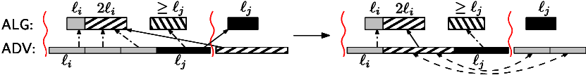
Figure 6: An illustration of the provisional assignment on the left; note that a packet of size $\ell_{j}$ with a forward charge is also assigned. Full arcs depict 1-to-1 charges and dashed arcs depict the provisional assignment. The result of modifying the adversary schedule on the right.

If $q\in Q$ receives a charge, it is a back charge from some packet $p$ of the same size. We remove $p$ from ADV and in the interval where $p$ was scheduled, we schedule packets from $f^{-1}(q)$ in an arbitrary order. As $\ell(f^{-1}(q))\leq\ell(q)$, this is feasible. If any packet $p\in f^{-1}(q)$ is charged, we keep its charge to the same packet in ${\textsf{PG\/}(s)}$; the charge was necessarily a forward charge, so it leads to some later block. See Figure 6 for an illustration.

After we have processed all the packets $q$, we have modified ADV by removing an allowed total size of packets and rescheduling the remaining packets in $(u,v]$ so that any remaining charges go to later blocks. This completes processing of the block $(u,v]$ and thus also the proof of 1-competitiveness.

5 Lower Bounds

5.1 Lower Bound with Two Packet Sizes

In this section we study lower bounds on the speed necessary to achieve 1-competitiveness. We start with a lower bound of 2 which holds even for the divisible case. It follows that our algorithm PG-DIV and the algorithm in Jurdzinski et al. [10] are optimal. Note that this lower bound follows from results of Anta et al. [2] by a similar construction, although the packets in their construction are not released together.

Theorem 5.1.

There is no 1-competitive deterministic online algorithm running with speed $s<2$, even if packets have sizes only $1$ and $\ell$ for $\ell>2s/(2-s)$ and all of them are released at time 0.

Proof.

For a contradiction, consider an algorithm ALG running with speed $s<2$ that is claimed to be 1-competitive with an additive constant $A$ where $A$ may depend on $\ell$. At time 0 the adversary releases $N_{1}=\lceil A/\ell\rceil+1$ packets of size $\ell$ and $\displaystyle{N_{0}=\left\lceil\frac{2\ell}{s}\cdot\big{(}N_{1}\cdot(s-1)\cdot\ell+A+1\big{)}\right\rceil}$ packets of size 1. These are all packets in the instance.

The adversary’s strategy works by blocks where a block is a time interval between two faults and the first block begins at time 0. The adversary ensures that in each such block ALG completes no packet of size $\ell$ and moreover ADV either completes an $\ell$-sized packet, or completes more $1$’s (packets of size $1$) than ALG.

Let $t$ be the time of the last fault; initially $t=0$. Let $\tau\geq t$ be the time when ALG starts the first $\ell$-sized packet after $t$ (or at $t$) if now fault occurs after $t$; we set $\tau=\infty$ if it does not happen. Note that we use here that ALG is deterministic. In a block beginning at time $t$, the adversary proceeds according to the first case below that applies.

1. If ADV has less than $2\ell/s$ pending packets of size 1, then the end of the schedule is at $t$.

2. If ADV has all packets of size $\ell$ completed, then it stops the current process and issues faults at times $t+1,t+2,\dots$ Between every two consecutive faults after $t$ it completes one packet of size 1 and it continues issuing faults until it has no pending packet of size 1. Then there is the end of the schedule. Clearly, ALG may complete only packets of size 1 after $t$ as $\ell>2s/(2-s)>s$ for $s<2$.

3. If $\tau\geq t+\ell/s-2$, then the next fault is at time $t+\ell$. In the current block, the adversary completes a packet $\ell$. ALG completes at most $s\cdot\ell$ packets of size 1 and then it possibly starts $\ell$ at $\tau$ (if $\tau<t+\ell$) which is jammed, since it would be completed at

   $$\tau+\frac{\ell}{s}\geq t+\frac{2\ell}{s}-2=t+\ell+\left(\frac{2}{s}-1\right)\ell-2>t+\ell$$

   where the last inequality follows from $\left(\frac{2}{s}-1\right)\ell>2$ which is equivalent to $\ell>2s/(2-s)$. Thus the $\ell$-sized packet would be completed after the fault. See Figure 8 for an illustration.

   

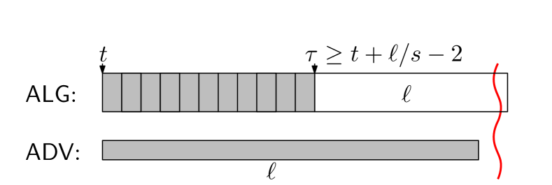
   Figure 7: An illustration of Case (D3).

   

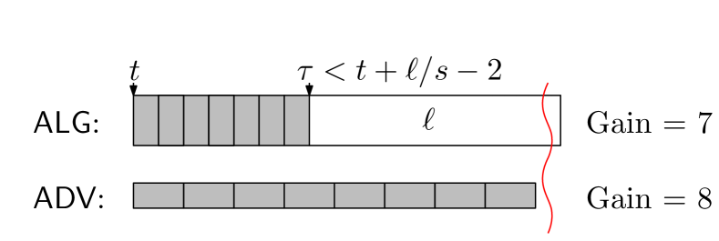
   Figure 8: An illustration of Case (D4).

4. Otherwise, if $\tau<t+\ell/s-2$, then the next fault is at time $\tau+\ell/s-\varepsilon$ for a small enough $\varepsilon>0$. In the current block, ADV completes as many packets of size 1 as it can, that is $\lfloor\tau+\ell/s-\varepsilon-t\rfloor$ packets of size 1; note that by Case (D1), ADV has enough 1’s pending. Again, the algorithm does not complete the packet of size $\ell$ started at $\tau$, because it would be finished at $\tau+\ell/s$. See Figure 8 for an illustration.

First notice that the process above ends, since in each block the adversary completes a packet. We now show $L_{\textsf{ADV\/}}>L_{\textsf{ALG\/}}+A$ which contradicts the claimed 1-competitiveness of ALG.

If the adversary’s strategy ends in Case (D2), then ADV has all $\ell$’s completed and then it schedules all 1’s, thus $L_{\textsf{ADV\/}}=N_{1}\cdot\ell+N_{0}>A+N_{0}$. However, ALG does not complete any $\ell$-sized packet and hence $L_{\textsf{ALG\/}}\leq N_{0}$ which concludes this case.

Otherwise, the adversary’s strategy ends in Case (D1). We first claim that in a block $(t,t^{\prime}]$ created in Case (D4), ADV  finishes more 1’s than ALG. Indeed, let $o$ be the number of 1’s completed by ALG in $(t,t^{\prime}]$. Then $\tau\geq t+o/s$ where $\tau$ is from the adversary’s strategy in $(t,t^{\prime}]$, and we also have $o<\ell-2s$ or equivalently $\ell>o+2s$, because $\tau<t+\ell/s-2$ in Case (D4). The number of 1’s scheduled by ADV is

$$\left\lfloor\tau+\frac{\ell}{s}-\varepsilon-t\right\rfloor \geq\left\lfloor t+\frac{o}{s}+\frac{\ell}{s}-\varepsilon-t\right\rfloor\geq\left\lfloor\frac{o}{s}+\frac{o+2s}{s}-\varepsilon\right\rfloor=\left\lfloor\frac{2}{s}o+2-\varepsilon\right\rfloor$$

$$\geq\left\lfloor\frac{2}{s}o+1\right\rfloor\geq o+1$$

and we proved the claim.

Let $\alpha$ be the number of blocks created in Case (D3); note that $\alpha\leq N_{1}$, since in each such block ADV finishes one $\ell$-sized packet. ALG completes at most $s\ell$ packets of size 1 in such a block, thus $L_{\textsf{ADV\/}}((u,v])-L_{\textsf{ALG\/}}((u,v])\geq(1-s)\cdot\ell$ for a block $(u,v]$ created in Case (D3).

Let $\beta$ be the number of blocks created in Case (D4). We have

$$\beta>\frac{s}{2\ell}\cdot\left(N_{0}-\frac{2\ell}{s}\right)=\frac{s\cdot N_{0}}{2\ell}-1=N_{1}\cdot(s-1)\cdot\ell+A\,,$$

because in each such block ADV schedules less than $2\ell/s$ packets of size 1 and less than $2\ell/s$ of these packets are pending at the end. By the claim above, we have $L_{\textsf{ADV\/}}((u,v])-L_{\textsf{ALG\/}}((u,v])\geq 1$ for a block $(u,v]$ created in Case (D4).

Summing over all blocks and using the value of $N_{0}$ we get

$$L_{\textsf{ADV\/}}-L_{\textsf{ALG\/}} \geq\alpha\cdot(1-s)\cdot\ell+\beta>N_{1}\cdot(1-s)\cdot\ell+N_{1}\cdot(s-1)\cdot\ell+A=A$$

where we used $s\geq 1$ which we may suppose w.l.o.g. This concludes the proof. ∎

5.2 Lower Bound for General Packet Sizes

Our main lower bound of $\phi+1=\phi^{2}\approx 2.618$ (where $\phi=(\sqrt{5}+1)/2$ is the golden ratio) generalizes the construction of Theorem 5.1 for more packet sizes, which are no longer divisible. Still, we make no use of release times.

Theorem 5.2.

There is no 1-competitive deterministic online algorithm running with speed $s<\phi+1$, even if all packets are released at time 0.

Outline of the proof

We start by describing the adversary’s strategy which works against an algorithm running at speed $s<\phi+1$, i.e., it shows that it is not $1$-competitive. It can be seen as a generalization of the strategy with two packet sizes above, but at the end the adversary sometimes needs a new strategy how to complete all short packets (of size less than $\ell_{i}$ for some $i$), preventing the algorithm to complete a long packet (of size at least $\ell_{i}$).

Then we show a few lemmata about the behavior of the algorithm. Finally, we prove that the gain of the adversary, i.e., the total size of its completed packets, is substantially larger than the gain of the algorithm.

Adversary’s strategy

The adversary chooses $\varepsilon>0$ small enough and $k\in\mathbb{N}$ large enough so that $s<\phi+1-1/\phi^{k-1}$. For convenience, the smallest size in the instance is $\varepsilon$ instead of $1$. There will be $k+1$ packet sizes in the instance, namely $\ell_{0}=\varepsilon$, and $\ell_{i}=\phi^{i-1}$ for $i=1,\dots,k$.

Suppose for a contradiction that there is an algorithm ALG running with speed $s<\phi+1$ that is claimed to be 1-competitive with an additive constant $A$ where $A$ may depend on $\ell_{i}$’s, in particular on $\varepsilon$ and $k$. The adversary issues $N_{i}$ packets of size $\ell_{i}$ at time 0, for $i=0,\dots,k$; $N_{i}$’s are chosen so that $N_{0}\gg N_{1}\gg\dots\gg N_{k}$. These are all packets in the instance.

More precisely, $N_{i}$’s are defined inductively so that it holds that $N_{k}>A/\ell_{k}$, $N_{i}>\phi s\ell_{k}\sum_{j=i+1}^{k}N_{j}+A/\ell_{i}$ for $i=k-1,\dots,1$, and finally

$$N_{0}>\frac{A+1+\phi\ell_{k}}{\varepsilon^{2}}\cdot\big{(}\phi s\ell_{k}\sum_{i=1}^{k}N_{i}\big{)}\,.$$

The adversary’s strategy works by blocks where a block is again a time interval between two faults and the first block begins at time 0. Let $t$ be the time of the last fault; initially $t=0$. Let $\tau_{i}\geq t$ be the time when ALG starts the first packet of size $\ell_{i}$ after $t$ (or at $t$) if no fault occurs after $t$; we set $\tau_{i}=\infty$ if it does not happen. Again, we use here that ALG is deterministic. Let $\tau_{\geq i}=\min_{j\geq i}\tau_{j}$ be the time when ALG starts the first packet of size at least $\ell_{i}$ after $t$. Let $P_{\textsf{ADV\/}}(i)$ be the total size of $\ell_{i}$’s (packets of size $\ell_{i}$) pending for the adversary at time $t$.

In a block beginning at time $t$, the adversary proceeds according to the first case below that applies. Each case has an intuitive explanation which we make precise later.

1. If there are less than $\phi\ell_{k}/\varepsilon$ packets of size $\varepsilon$ pending for ADV, then the end of the schedule is at time $t$.

   Lemma 5.3 below shows that in blocks in which ADV schedules $\varepsilon$’s it completes more than ALG in terms of total size. It follows that the schedule of ADV has much larger total completed size for $N_{0}$ large enough, since the adversary scheduled nearly all packets of size $\varepsilon$; see Lemma 5.8.

2. If there is $i\geq 1$ such that $P_{\textsf{ADV\/}}(i)=0$, then ADV stops the current process and continues by Strategy Finish described below.

3. If $\tau_{1}<t+\ell_{1}/(\phi\cdot s)$, then the next fault occurs at time $\tau_{1}+\ell_{1}/s-\varepsilon$, so that ALG does not finish the first $\ell_{1}$-sized packet. ADV schedules as many $\varepsilon$’s as it can.

   In this case, ALG schedules $\ell_{1}$ too early and in Lemma 5.3 we show that the total size of packets completed by ADV is larger than the total size of packets completed by ALG.

4. If $\tau_{\geq 2}<t+\ell_{2}/(\phi\cdot s)$, then the next fault is at time $\tau_{\geq 2}+\ell_{2}/s-\varepsilon$, so that ALG does not finish the first packet of size at least $\ell_{2}$. ADV again schedules as many $\varepsilon$’s as it can. Similarly as in the previous case, ALG starts $\ell_{2}$ or a larger packet too early and we show that ADV completes more in terms of size than ALG, again using Lemma 5.3.

5. If there is $1\leq i<k$ such that $\tau_{\geq i+1}<\tau_{i}$, then we choose the smallest such $i$ and the next fault is at time $t+\ell_{i}$. ADV schedules a packet of size $\ell_{i}$. See Figure 10 for an illustration.

   Intuitively, this case means that ALG skips $\ell_{i}$ and schedules $\ell_{i+1}$ (or a larger packet) earlier. Lemma 5.5 shows that the algorithm cannot finish its first packet of size at least $\ell_{i+1}$ (thus it also does not schedule $\ell_{i}$) provided that this case is not triggered for a smaller $i$, or previous cases are not triggered.

   

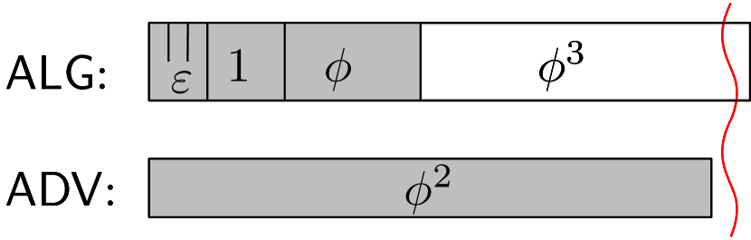
   Figure 9: An illustration of Case (B5).

   

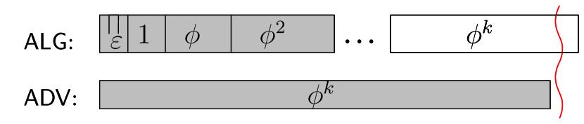
   Figure 10: An illustration of Case (B6).

6. Otherwise, the next fault occurs at $t+\ell_{k}$ and ADV schedules a packet of size $\ell_{k}$ in this block. Lemma 5.6 shows that ALG cannot complete an $\ell_{k}$-sized packet in this block. See Figure 10 for an illustration.

We remark that the process above eventually ends either in Case (B1), or in Case (B2), since in each block ADV schedules a packet. Also note that the length of each block is at most $\phi\ell_{k}$.

We describe Strategy Finish, started in Case (B2). Let $i$ be the smallest index $i^{\prime}\geq 1$ such that $P_{\textsf{ADV\/}}(i^{\prime})=0$. For brevity, we call a packet of size at least $\ell_{i}$ long, and a packet of size $\ell_{j}$ with $1\leq j<i$ short; note that $\varepsilon$’s are not short packets. In a nutshell, ADV tries to schedule all short packets, while preventing the algorithm from completing any long packet. Similarly to Cases (B3) and (B4), if ALG is starting a long packet too early, ADV schedules $\varepsilon$’s and gains in terms of total size.

Adversary’s Strategy Finish works again by blocks. Let $t$ be the time of the last fault. Let $\tau\geq t$ be the time when ALG starts the first long packet after $t$; we set $\tau=\infty$ if it does not happen. The adversary proceeds according to the first case below that applies:

1. If $P_{\textsf{ADV\/}}(0)<\phi\ell_{k}$, then the end of the schedule is at time $t$.

2. If ADV has no pending short packet, then the strategy Finish ends and ADV issues faults at times $t+\varepsilon,t+2\varepsilon,\dots$ Between every two consecutive faults after $t$ it completes one packet of size $\varepsilon$ and it continues issuing faults until it has no pending $\varepsilon$. Then there is the end of the schedule. Clearly, ALG may complete only $\varepsilon$’s after $t$ if $\varepsilon$ is small enough. Note that for $i=1$ this case is immediately triggered, as $\ell_{0}$-sized packets are not short, hence there are no short packets whatsoever.

3. If $\tau<t+\ell_{i}/(\phi\cdot s)$, then the next fault is at time $\tau+\ell_{i}/s-\varepsilon$, so that ALG does not finish the first long packet. ADV schedules as many $\varepsilon$’s as it can. Note that the length of this block is less than $\ell_{i}/(\phi\cdot s)+\ell_{i}/s\leq\phi\ell_{k}$. Again, we show that ADV completes more in terms of size using Lemma 5.3.

4. Otherwise, $\tau\geq t+\ell_{i}/(\phi\cdot s)$. ADV issues the next fault at time $t+\ell_{i-1}$. Let $j$ be the largest $j^{\prime}<i$ such that $P_{\textsf{ADV\/}}(j^{\prime})>0$. ADV schedules a packet of size $\ell_{j}$ which is completed as $j\leq i-1$. Lemma 5.7 shows that ALG does not complete the long packet started at $\tau$.

Again, in each block ADV completes a packet, thus Strategy Finish eventually ends. Note that the length of each block is less than $\phi\ell_{k}$.

Properties of the adversary’s strategy

We now prove the lemmata mentioned above. In the following, $t$ is the beginning of the considered block and $t^{\prime}$ is the end of the block, i.e., the time of the next fault after $t$. Recall that $L_{\textsf{ALG\/}}((t,t^{\prime}])$ is the total size of packets completed by ALG in $(t,t^{\prime}]$. We start with a general lemma that covers all cases in which ADV schedules many $\varepsilon$’s.

Lemma 5.3.

In Cases (B3), (B4), and (F3), $L_{\textsf{ADV\/}}((t,t^{\prime}])\geq L_{\textsf{ALG\/}}((t,t^{\prime}])+\varepsilon$ holds.

Proof.

Let $i$ and $\tau$ be as in Case (F3); we set $i=1$ and $\tau=\tau_{1}$ in Case (B3), and $i=2$ and $\tau=\tau_{\geq 2}$ in Case (B4). Note that the first packet of size (at least) $\ell_{i}$ is started at $\tau$ with $\tau<t+\ell_{i}/(\phi\cdot s)$ and that the next fault occurs at time $\tau+\ell_{i}/s-\varepsilon$. Furthermore, $P_{\textsf{ADV\/}}(0,t)\geq\phi\ell_{k}$ by Cases (B1) and (F1). As $t^{\prime}-t\leq\phi\ell_{k}$ it follows that ADV has enough $\varepsilon$’s to fill nearly the whole block with them, so in particular $L_{\textsf{ADV\/}}((t,t^{\prime}])>t^{\prime}-t-\varepsilon$.

Let $a=L_{\textsf{ALG\/}}((t,t^{\prime}])$. Since ALG does not complete the $\ell_{i}$-sized packet we have $\tau\geq t+a/s$ and thus also $a<\ell_{i}/\phi$ as $\tau<t+\ell_{i}/(\phi\cdot s)$.

If $a<\ell_{i}/\phi-3s\varepsilon/\phi$ which is equivalent to $\ell_{i}>\phi\cdot a+3s\varepsilon$, then we show the required inequality by the following calculation:

$$L_{\textsf{ADV\/}}((t,t^{\prime}])+\varepsilon>t^{\prime}-t=\tau+\frac{\ell_{i}}{s}-\varepsilon-t\geq\frac{a}{s}+\frac{\ell_{i}}{s}-\varepsilon>\frac{a+\phi\cdot a+3s\varepsilon}{s}-\varepsilon>a+2\varepsilon\,,$$

where the last inequality follows from $s<\phi+1$.

Otherwise, $a$ is nearly $\ell_{i}/\phi$ and thus large enough. Then we get

$$L_{\textsf{ADV\/}}((t,t^{\prime}])+\varepsilon>t^{\prime}-t=\tau+\frac{\ell_{i}}{s}-\varepsilon-t\geq\frac{a}{s}+\frac{\ell_{i}}{s}-\varepsilon>\frac{a}{s}+\frac{\phi a}{s}-\varepsilon>a+2\varepsilon$$

where the penultimate inequality follows by $\ell_{i}>\phi a$, and the last inequality holds as $(1+\phi)a/s>a+3\varepsilon$ for $\varepsilon$ small enough and $a\geq\ell_{i}/\phi-3s\varepsilon/\phi$. ∎

For brevity, we inductively define $S_{0}=\phi-1$ and $S_{i}=S_{i-1}+\ell_{i}$ for $i=1,\dots,k$. Thus $S_{i}=\sum_{j=1}^{i}\ell_{i}+\phi-1$ and a calculation shows $S_{i}=\phi^{i+1}-1$. We prove a useful observation.

Lemma 5.4.

Fix $j\geq 2$. If Case (B3) and Case (B5) for $i<j$ are not triggered in the block, then $\tau_{i^{\prime}+1}\geq t+S_{i^{\prime}}/s$ for each $i^{\prime}<j$.

Proof.

We have $\tau_{1}\geq t+\ell_{1}/(\phi\cdot s)=t+(\phi-1)/s$ by Case (B3) and $\tau_{i+1}\geq\tau_{i}+\ell_{i}/s$ for any $i<j$, since Case (B5) was not triggered for $i<j$ and the first $\ell_{i}$-sized packet needs to be finished before starting the next packet. Summing the bounds gives the inequalities in the lemma. ∎

Lemma 5.5.

In Case (B5), the algorithm does not complete any packet of size $\ell_{i}$ or larger.

Proof.

Recall that we have $\tau_{\geq i+1}<\tau_{i}$, thus the first started packet $p$ of size at least $\ell_{i}$ has size at least $\ell_{i+1}$. It suffices to prove

$$\tau_{\geq i+1}+\frac{\ell_{i+1}}{s}-t>\ell_{i}\,,$$ (5.1)

which means that $p$ would be completed after the next fault at time $t+\ell_{i}$.

We start with the case $i=1$ in which $\tau_{\geq 2}<\tau_{1}$. Since Case (B4) was not triggered, we have $\tau_{\geq 2}\geq t+\ell_{2}/(\phi\cdot s)=t+1/s$. We show (5.1) by the following calculation:

$$\tau_{\geq 2}+\frac{\ell_{2}}{s}-t\geq\frac{1}{s}+\frac{\ell_{2}}{s}=\frac{1+\phi}{s}>1=\ell_{1}\enspace,$$

where the strict inequality holds by $s<\phi+1$.

Now consider the case $i\geq 2$. By the minimality of $i$ satisfying the condition of Case (B5), we use Lemma 5.4 for $j=i$ and $i^{\prime}=i-2$ to get $\tau_{i-1}\geq t+S_{i-2}/s$. Since a packet $\ell_{i-1}$ is started at $\tau_{i-1}$ and must be finished by $\tau_{\geq i+1}$, it holds $\tau_{\geq i+1}\geq t+(S_{i-2}+\ell_{i-1})/s=t+S_{i-1}/s$. Thus

$$\tau_{\geq i+1}+\frac{\ell_{i+1}}{s}-t\geq\frac{S_{i-1}+\ell_{i+1}}{s} =\frac{\phi^{i}-1+\phi^{i}}{s}$$

$$=\frac{\phi^{i+1}+\phi^{i-2}-1}{s}\geq\frac{\phi^{i+1}}{s}>\phi^{i-1}=\ell_{i}\,,$$

where the penultimate inequality holds by $i\geq 2$ and the last inequality by $s<\phi+1$. (We remark that the penultimate inequality has a significant slack for $i>2$.) ∎

Lemma 5.6.

In Case (B6), ALG does not complete a packet of size $\ell_{k}$.

Proof.

It suffices to prove

$$\tau_{k}>t+\left(1-\frac{1}{s}\right)\ell_{k}\,,$$ (5.2)

since then ALG completes the first $\ell_{k}$-sized packet at

$$\tau_{k}+\frac{\ell_{k}}{s}>t+\left(1-\frac{1}{s}\right)\ell_{k}+\frac{\ell_{k}}{s}=t+\ell_{k}\,,$$

i.e., after the next fault at time $t+\ell_{k}$.

Recall that we choose $k$ large enough so that $s<\phi+1-1/\phi^{k-1}$ or equivalently $\phi-1/\phi^{k-1}>s-1$. We multiply the inequality by $\phi^{k-1}$, divide it by $s$ and add $t$ to both sides and we get

$$t+\frac{\phi^{k}-1}{s}>t+\left(1-\frac{1}{s}\right)\phi^{k-1}=t+\left(1-\frac{1}{s}\right)\ell_{k}\,.$$ (5.3)

Since Cases (B3) and (B5) are not triggered, we use Lemma 5.4 for $j=k$ to show $\tau_{k}\geq t+S_{k-1}/s=t+(\phi^{k}-1)/s$. We combine this with (5.3) and we have

$$\tau_{k}\geq t+\frac{\phi^{k}-1}{s}>t+\left(1-\frac{1}{s}\right)\ell_{k}\,,$$ (5.4)

which shows (5.2) and concludes the proof of the lemma. ∎

Lemma 5.7.

In Case (F4), ALG does not complete any long packet.

Proof.

Recall that the first long packet $p$ is started at $\tau$ and it has size of at least $\ell_{i}$, thus it would be completed at $\tau+\ell_{i}/s$ or later. We show $\tau+\ell_{i}/s-t>\ell_{i-1}$ by the following calculation:

$$\tau+\frac{\ell_{i}}{s}-t\geq\frac{\ell_{i}}{\phi\cdot s}+\frac{\ell_{i}}{s}=\frac{\phi\ell_{i}}{s}>\frac{\ell_{i}}{\phi}=\ell_{i-1}\,,$$

where the strict inequality holds by $s<\phi+1$. This implies that the long packet $p$ would be completed after the next fault at time $t+\ell_{i-1}$. ∎

Analysis of the gains

We are ready to prove that at the end of the schedule $L_{\textsf{ADV\/}}>L_{\textsf{ALG\/}}+A$ holds, which contradicts the claimed 1-competitiveness of ALG and proves Theorem 5.2. We inspect all the cases in which the instances may end, starting with Cases (B1) and (F1). We remark that we use only crude bounds to keep the analysis simple.

Lemma 5.8.

If the schedule ends in Case (B1) or (F1), we have $L_{\textsf{ADV\/}}>L_{\textsf{ALG\/}}+A$.

Proof.

Recall that each block $(t,t^{\prime}]$ has length of at most $\phi\ell_{k}$, thus $L_{\textsf{ALG\/}}((t,t^{\prime}])\leq s\phi\ell_{k}$ and $L_{\textsf{ADV\/}}((t,t^{\prime}])\leq\phi\ell_{k}$.

We call a block in which ADV schedules many $\varepsilon$’s small, other blocks are big. Recall that ADV schedules no $\varepsilon$ in a big block. Note that Cases (B3), (B4), and (F3) concern small blocks, whereas Cases (B5), (B6), and (F4) concern big blocks.

By Lemma 5.3, in each small block $(t,t^{\prime}]$ it holds that $L_{\textsf{ADV\/}}((t,t^{\prime}])\geq L_{\textsf{ALG\/}}((t,t^{\prime}])+\varepsilon$. Let $\beta$ be the number of small blocks. We observe that

$$\beta\geq\frac{\left(N_{0}-\frac{\phi\ell_{k}}{\varepsilon}\right)\varepsilon}{\phi\ell_{k}}\,,$$

because in each such block ADV schedules at most $\phi\ell_{k}/\varepsilon$ packets of size $\varepsilon$ and $P_{\textsf{ADV\/}}(0)<\phi\ell_{k}$ at the end in Cases (B1) and (F1).

The number of big blocks is at most $\sum_{i=1}^{k}N_{i}$, since in each such block ADV schedules a packet of size at least $\ell_{1}$. For each such block we have $L_{\textsf{ADV\/}}((t,t^{\prime}])-L_{\textsf{ALG\/}}((t,t^{\prime}])\geq-s\phi\ell_{k}$ which is only a crude bound, but it suffices for $N_{0}$ large enough.

Summing over all blocks we obtain

$$L_{\textsf{ADV\/}}-L_{\textsf{ALG\/}} \geq\beta\varepsilon-\phi s\ell_{k}\sum_{i=1}^{k}N_{i}\geq\frac{\left(N_{0}-\frac{\phi\ell_{k}}{\varepsilon}\right)\varepsilon^{2}}{\phi\ell_{k}}-\phi s\ell_{k}\sum_{i=1}^{k}N_{i}$$

$$>A+\phi s\ell_{k}\sum_{i=1}^{k}N_{i}-\phi s\ell_{k}\sum_{i=1}^{k}N_{i}=A\enspace,$$ (5.5)

where (5.5) follows from $N_{0}>\phi\ell_{k}(A+1+\phi s\ell_{k}\sum_{i=1}^{k}N_{i})/\varepsilon^{2}$. ∎

It remains to prove the same for termination by Case (F2), since there is no other case in which the strategy may end.

Lemma 5.9.

If Strategy Finish ends in Case (F2), then $L_{\textsf{ADV\/}}>L_{\textsf{ALG\/}}+A$.

Proof.

Note that ADV schedules all short packets and all $\varepsilon$’s, i.e., those of size less than $\ell_{i}$. In particular, we have $L_{\textsf{ADV\/}}(<i)\geq L_{\textsf{ALG\/}}(<i)$.

Call a block in which ALG completes a packet of size at least $\ell_{i}$ bad. As the length of any block is at most $\phi\ell_{k}$ we get that $L_{\textsf{ALG\/}}(\geq i,(t,t^{\prime}])\leq s\phi\ell_{k}$ for a bad block $(t,t^{\prime}]$. Bad blocks are created only in Cases (B5) and (B6), but in each bad block ADV finishes a packet strictly larger than $\ell_{i}$; note that here we use Lemmata 5.5 and 5.6. Hence the number of bad blocks is bounded by $\sum_{j=i+1}^{k}N_{j}$. As ADV completes all $\ell_{i}$’s we obtain

$$L_{\textsf{ADV\/}}(\geq i)-L_{\textsf{ALG\/}}(\geq i) \geq\ell_{i}N_{i}-\phi s\ell_{k}\sum_{j=i+1}^{k}N_{j}$$

$$>\ell_{i}\phi s\ell_{k}\sum_{j=i+1}^{k}N_{j}+A-\phi s\ell_{k}\sum_{j=i+1}^{k}N_{j}\geq A\,,$$

where the strict inequality follows from $N_{k}>A/\ell_{k}$ for $i=k$ and from $N_{i}>\phi s\ell_{k}\sum_{j=i+1}^{k}N_{j}+A/\ell_{i}$ for $i<k$. By summing it with $L_{\textsf{ADV\/}}(<i)\geq L_{\textsf{ALG\/}}(<i)$ we conclude that $L_{\textsf{ADV\/}}>L_{\textsf{ALG\/}}+A$. ∎

References

- [1] Antonio Fernández Anta, Chryssis Georgiou, Dariusz R. Kowalski, Joerg Widmer, and Elli Zavou. Measuring the impact of adversarial errors on packet scheduling strategies. J. Scheduling, 19(2):135–152, 2016. Also appeared in Proc. of SIROCCO 2013: 261–273. doi:10.1007/s10951-015-0451-z.
- [2] Antonio Fernández Anta, Chryssis Georgiou, Dariusz R. Kowalski, and Elli Zavou. Online parallel scheduling of non-uniform tasks: Trading failures for energy. Theor. Comput. Sci., 590:129–146, 2015. Also appeared in Proc. of FCT 2013: 145-158. doi:10.1016/j.tcs.2015.01.027.
- [3] Antonio Fernández Anta, Chryssis Georgiou, Dariusz R. Kowalski, and Elli Zavou. Competitive analysis of fundamental scheduling algorithms on a fault-prone machine and the impact of resource augmentation. Future Generation Comp. Syst., 78:245–256, 2018. Also appeared in Proc. of ARMS-CC@PODC 2015, LNCS 9438: 1–16. doi:10.1016/j.future.2016.05.042.
- [4] Shai Ben-David, Allan Borodin, Richard M. Karp, Gábor Tardos, and Avi Wigderson. On the power of randomization in on-line algorithms. Algorithmica, 11(1):2–14, 1994. Also appeared in Proc. of STOC 1990: 379–386. doi:10.1007/BF01294260.
- [5] Martin Böhm, Łukasz Jeż, Jiří Sgall, and Pavel Veselý. On packet scheduling with adversarial jamming and speedup. In Proc. of the 15th Workshop on Approximation and Online Algorithms (WAOA’17), volume 10787 of LNCS, pages 190–206, 2018. doi:10.1007/978-3-319-89441-6_15.
- [6] Allan Borodin and Ran El-Yaniv. Online computation and competitive analysis. Cambridge University Press, 1998.
- [7] Marek Chrobak, Leah Epstein, John Noga, Jiří Sgall, Rob van Stee, Tomáš Tichý, and Nodari Vakhania. Preemptive scheduling in overloaded systems. J. Comput. Syst. Sci., 67:183–197, 2003. doi:10.1016/S0022-0000(03)00070-9.
- [8] P. Garncarek, T. Jurdziński, and K. Loryś. Fault-tolerant online packet scheduling on parallel channels. In 2017 IEEE International Parallel and Distributed Processing Symposium (IPDPS), pages 347–356, May 2017. doi:10.1109/IPDPS.2017.105.
- [9] Chryssis Georgiou and Dariusz R. Kowalski. On the competitiveness of scheduling dynamically injected tasks on processes prone to crashes and restarts. J. Parallel Distrib. Comput., 84:94–107, 2015. doi:10.1016/j.jpdc.2015.07.007.
- [10] Tomasz Jurdzinski, Dariusz R. Kowalski, and Krzysztof Loryś. Online packet scheduling under adversarial jamming. In Proc. of the 12th Workshop on Approximation and Online Algorithms (WAOA’14), volume 8952 of LNCS, pages 193–206, 2015. See http://arxiv.org/abs/1310.4935 for missing proofs. doi:10.1007/978-3-319-18263-6_17.
- [11] Bala Kalyanasundaram and Kirk Pruhs. Speed is as powerful as clairvoyance. J. of the ACM, 47(4):617–643, 2000. Also appeared in Proc. of FOCS 1995: 214–221. doi:10.1145/347476.347479.
- [12] Chiu-Yuen Koo, Tak Wah Lam, Tsuen-Wan Ngan, Kunihiko Sadakane, and Kar-Keung To. On-line scheduling with tight deadlines. Theor. Comput. Sci., 295:251–261, 2003. doi:10.1016/S0304-3975(02)00407-3.
- [13] Dariusz R. Kowalski, Prudence W. H. Wong, and Elli Zavou. Fault tolerant scheduling of tasks of two sizes under resource augmentation. Journal of Scheduling, 20(6):695–711, Dec 2017. doi:10.1007/s10951-017-0541-1.
- [14] Tak Wah Lam, Tsuen-Wan Ngan, and Kar-Keung To. Performance guarantee for EDF under overload. J. Algorithms, 52:193–206, 2004. doi:10.1016/j.jalgor.2003.10.004.
- [15] Tak Wah Lam and Kar-Keung To. Trade-offs between speed and processor in hard-deadline scheduling. In Proc. of the 10th Annual ACM-SIAM Symposium on Discrete Algorithms (SODA’99), pages 623–632. ACM/SIAM, 1999. URL: http://dl.acm.org/citation.cfm?id=314500.314884.
- [16] Cynthia A. Phillips, Clifford Stein, Eric Torng, and Joel Wein. Optimal time-critical scheduling via resource augmentation. Algorithmica, 32:163–200, 2002. Also appeared in Proc. of STOC 1997: 140–149. doi:10.1007/s00453-001-0068-9.
- [17] Kirk Pruhs. Competitive online scheduling for server systems. SIGMETRICS Performance Evaluation Review, 34(4):52–58, 2007. doi:10.1145/1243401.1243411.
- [18] Kevin Schewior. Handling Critical Tasks Online: Deadline Scheduling and Convex-Body Chasing. PhD dissertation, TU Berlin, 2016. URL: http://dx.doi.org/10.14279/depositonce-5427.
- [19] Daniel Dominic Sleator and Robert Endre Tarjan. Amortized efficiency of list update and paging rules. Commun. ACM, 28(2):202–208, 1985. doi:10.1145/2786.2793.