R Package ASMap: Efficient Genetic Linkage Map Construction and Diagnosis

Julian Taylor, David Butler R Package ASMap: Efficient Genetic Linkage Map Construction and Diagnosis Linkage Map Construction and Diagnosis Although various forms of linkage map construction software are widely available, there is a distinct lack of packages for use in the R statistical computing environment (rsoft15). This article introduces the ASMap linkage map construction R package which contains functions that use the efficient MSTmap algorithm (mst08) for clustering and optimally ordering large sets of markers. Additional to the construction functions, the package also contains a suite of tools to assist in the rapid diagnosis and repair of a constructed linkage map. The package functions can also be used for post linkage map construction techniques such as fine mapping or combining maps of the same population. To showcase the efficiency and functionality of ASMap, the complete linkage map construction process is demonstrated with a high density barley backcross marker data set. linkage map construction, genetics, quantitative trait loci, R linkage map construction, genetics, quantitative trait loci, R Julian Taylor
School of Agriculture, Food & Wine
The University of Adelaide
PMB 1, Glen Osmond, SA, 5064, Australia
E-mail:

David Butler
Department of Agriculture, Fisheries & Forestry
Queensland Government
PMB 102, Toowoomba, QLD, 4350, Australia
E-mail:

1 Introduction

Genetic linkage maps are widely used in the biological research community to explore the underlying DNA of populations. They generally consist of a set of polymorphic genetic markers spanning the entire genome of a population generated from a specific cross of parental lines. This exploration may involve the dissection of the linkage map itself to understand the genetic landscape of the population or, more commonly, it is used to conduct gene-trait associations such as quantitative trait loci (QTL) analysis or genomic selection (GS). For QTL analysis, the interpretation of significant genomic locations is enhanced if the linkage map contains markers that have been assigned and optimally ordered within chromosomal groups. This can be achieved algorithmically by using linkage map construction techniques that utilise the laws of Mendelian genetics (stur13).

In the relatively short history of linkage map construction there has been an abundance of stand alone software. Early linkage map construction algorithms used brute force combinatoric methods to determine marker order (lg87; lw89) and were built into historical versions of popular software packages Mapmaker (land87) and JoinMap (stam93). As the number of markers increased non-combinatoric methods emerged, including SERIATION (ser87) and Rapid Chain Delineation (RCD) (doe96). A version of RCD was implemented in the intuitive graphically oriented package Map Manager. (man01). Although Map Manager enjoyed a meteoric rise in use, the implemented RCD algorithm was sub-optimal and the software was limited to reduced numbers of markers. car97 and liu98 recognised a more efficient approach to marker ordering could be attained from finding solutions to the travelling salesman problem. Computational methods that exploited this knowledge were quickly adopted in construction algorithms including the Evolution-Strategy algorithm (mest03; mest03a) implemented in Multipoint and the RECORD algorithm (rec05) available as command line software and later implemented in software packages IciMapping (meng15) and onemap (one15). Other construction algorithm variants involving efficient solutions of the travelling salesman problem included the unidirectional growth (UG) algorithm (tf06), AntMap algorithm (in06), the MSTmap algorithm (mst08) and Lep-MAP (ras13). Unfortunately these more recent algorithms have only been available as downloadable low-level source code that require compilation before use.

In the R statistical computing environment there were only two packages available for linkage map construction. The qtl package (br15; brosen09) has matured considerably since it inception in 2001 and provides users with a suite of functions for linkage map construction and QTL analysis across a wide set of populations. Unfortunately, the marker ordering algorithms in the package rely on computationally cumbersome combinatoric methods and multiple stages to achieve optimality. In a more recent addition to the R contributed package list, onemap (one15) contains a collection of linkage map construction tools specialized for a restricted set of inbred and outbred populations. The package implements well known marker ordering algorithms including SERIATION (ser87), RECORD (rec05), RCD (doe96) and UG (tf06). Unfortunately these algorithms have been implemented in native R code and lack the computational expediency of the low-level source code equivalents.

In an attempt to circumvent these computational issues we developed the ASMap package (tb15) which is freely downloadable at http://CRAN.R-project.org/package=ASMap. The package contains linkage map construction functions that fully utilize the freely available C++ source code (http://alumni.cs.ucr.edu/~yonghui/mstmap.html) for the MSTmap algorithm derived in mst08 and outlined in Section 2. The algorithm uses the minimum spanning tree of a graph (ct76) to cluster markers into linkage groups as well as find the optimal marker order within each linkage group. In contrast to qtl and onemap, genetic linkage maps are constructed very efficiently without the requirement for multiple ordering stages. The algorithm is restricted to linkage map construction with Backcross (BC), Doubled Haploid (DH) and Recombinant Inbred (RIL) populations. For RIL populations, the level of self pollination can also be given and consequently the algorithm can handle selfed F2, F3, $\ldots$, F$r$ populations where $r$ is the level of selfing. Advanced RIL populations $(r\rightarrow\infty)$ are also allowed and are treated similar to a DH population for the purpose of linkage map construction.

An overview of the ASMap package functions are presented in Section 3. Two linkage map construction functions are available that provide users with a fast, flexible set of tools for constructing linkage maps using the MSTmap algorithm. To complement the efficient construction functions the package also contains a function that pulls markers of different types from the linkage map, temporarily placing them aside. This is complemented by a function that pushes markers back to linkage groups at any stage of the construction or reconstruction process. To efficiently diagnose the quality of the constructed map the package contains graphical functions that simultaneously display multiple panel profiles of linkage map statistics associated with the genotypes or marker/intervals. Where possible, the ASMap package uses the "cross" object format (see the qtl function read.cross() for the structure of its genetic objects. Once the class of the object is appropriately set, both ASMap and qtl functions can be used synergistically to construct, explore and manipulate the object. To showcase the functionality of the ASMap package, Section 4 presents an illustrative example that involves the complete linkage map construction process for a barley Backcross population. This section concludes with a short summary on the use of ASMap functions in post construction linkage map development techniques such as fine mapping and combining maps. The performance of the MSTmap algorithm in ASMap is outlined in Section LABEL:sec:lim and the article concludes with a short summary.

2 MSTmap algorithm

Following the notation of mst08 consider a Doubled Haploid population of $n$ individuals genotyped across a set of $t$ markers where each $(j,k)$th entry of the $n\times t$ matrix $\textstyle{M}$ is either an $A$ or a $B$ representing the two parental homozygotes in the population. Let ${\mathchoice{\hbox{\boldmath$\displaystyle{P}$}}{\hbox{\boldmath$\textstyle{P}$}}{\hbox{\boldmath$\scriptstyle{P}$}}{\hbox{\boldmath$\scriptscriptstyle{P}$}}}_{jk}$ be the probability of a recombination event between the markers $({\mathchoice{\hbox{\boldmath$\displaystyle{m}$}}{\hbox{\boldmath$\textstyle{m}$}}{\hbox{\boldmath$\scriptstyle{m}$}}{\hbox{\boldmath$\scriptscriptstyle{m}$}}}_{j},{\mathchoice{\hbox{\boldmath$\displaystyle{m}$}}{\hbox{\boldmath$\textstyle{m}$}}{\hbox{\boldmath$\scriptstyle{m}$}}{\hbox{\boldmath$\scriptscriptstyle{m}$}}}_{k})$ where $0\leq{\mathchoice{\hbox{\boldmath$\displaystyle{P}$}}{\hbox{\boldmath$\textstyle{P}$}}{\hbox{\boldmath$\scriptstyle{P}$}}{\hbox{\boldmath$\scriptscriptstyle{P}$}}}_{jk}\leq 0.5$. MSTmap uses two possible weight objective functions based on recombination probabilities between the markers

$$w_{p}(j,k) ={\mathchoice{\hbox{\boldmath$\displaystyle{P}$}}{\hbox{\boldmath$\textstyle{P}$}}{\hbox{\boldmath$\scriptstyle{P}$}}{\hbox{\boldmath$\scriptscriptstyle{P}$}}}_{jk}$$ (1)

$$w_{ml}(j,k) =-\bigl{(}{\mathchoice{\hbox{\boldmath$\displaystyle{P}$}}{\hbox{\boldmath$\textstyle{P}$}}{\hbox{\boldmath$\scriptstyle{P}$}}{\hbox{\boldmath$\scriptscriptstyle{P}$}}}_{jk}\log\,{\mathchoice{\hbox{\boldmath$\displaystyle{P}$}}{\hbox{\boldmath$\textstyle{P}$}}{\hbox{\boldmath$\scriptstyle{P}$}}{\hbox{\boldmath$\scriptscriptstyle{P}$}}}_{jk}+(1-{\mathchoice{\hbox{\boldmath$\displaystyle{P}$}}{\hbox{\boldmath$\textstyle{P}$}}{\hbox{\boldmath$\scriptstyle{P}$}}{\hbox{\boldmath$\scriptscriptstyle{P}$}}}_{jk})\log(\,1-{\mathchoice{\hbox{\boldmath$\displaystyle{P}$}}{\hbox{\boldmath$\textstyle{P}$}}{\hbox{\boldmath$\scriptstyle{P}$}}{\hbox{\boldmath$\scriptscriptstyle{P}$}}}_{jk})\bigr{)}$$ (2)

In general ${\mathchoice{\hbox{\boldmath$\displaystyle{P}$}}{\hbox{\boldmath$\textstyle{P}$}}{\hbox{\boldmath$\scriptstyle{P}$}}{\hbox{\boldmath$\scriptscriptstyle{P}$}}}_{jk}$ is not known and so it is replaced by an estimate, $d_{jk}/n$ where $d_{jk}$ corresponds to the hamming distance between ${\mathchoice{\hbox{\boldmath$\displaystyle{m}$}}{\hbox{\boldmath$\textstyle{m}$}}{\hbox{\boldmath$\scriptstyle{m}$}}{\hbox{\boldmath$\scriptscriptstyle{m}$}}}_{j}$ and ${\mathchoice{\hbox{\boldmath$\displaystyle{m}$}}{\hbox{\boldmath$\textstyle{m}$}}{\hbox{\boldmath$\scriptstyle{m}$}}{\hbox{\boldmath$\scriptscriptstyle{m}$}}}_{k}$ (the number of non-matching alleles between the two markers). This estimate, $d_{jk}/n$, is also the maximum likelihood estimate for ${\mathchoice{\hbox{\boldmath$\displaystyle{P}$}}{\hbox{\boldmath$\textstyle{P}$}}{\hbox{\boldmath$\scriptstyle{P}$}}{\hbox{\boldmath$\scriptscriptstyle{P}$}}}_{jk}$ for the two weight functions defined above.

2.1 Clustering

If markers ${\mathchoice{\hbox{\boldmath$\displaystyle{m}$}}{\hbox{\boldmath$\textstyle{m}$}}{\hbox{\boldmath$\scriptstyle{m}$}}{\hbox{\boldmath$\scriptscriptstyle{m}$}}}_{j}$ and ${\mathchoice{\hbox{\boldmath$\displaystyle{m}$}}{\hbox{\boldmath$\textstyle{m}$}}{\hbox{\boldmath$\scriptstyle{m}$}}{\hbox{\boldmath$\scriptscriptstyle{m}$}}}_{k}$ belong to two different linkage groups then ${\mathchoice{\hbox{\boldmath$\displaystyle{P}$}}{\hbox{\boldmath$\textstyle{P}$}}{\hbox{\boldmath$\scriptstyle{P}$}}{\hbox{\boldmath$\scriptscriptstyle{P}$}}}_{jk}=0.5$ and the hamming distance between them has the property $E(d_{jk})=n/2$. Using these definitions, MSTmap determines whether markers belong to the same linkage group using Hoeffdings inequality

$$P(d_{jk}<\delta)\leq\mbox{exp}(-2(n/2-\delta)^{2}/n)$$ (3)

for $\delta<n/2$. For a given $P(d_{jk}<\delta)=\epsilon$ and $n$, the equation $-2(n/2-\delta)^{2}/n=\mbox{log}\,\epsilon$ is solved to determine an appropriate hamming distance threshold, $\hat{\delta}$. mst08 indicate that the choice of $\epsilon$ is not crucial when attempting to form linkage groups. However, the equation that requires solving is highly dependent on the number of individuals in the population. For example, for a DH population, Figure 1 shows the profiles of the negative $\log 10\epsilon$ against the number of individuals in the population for four threshold minimum cM distances $(25,30,35,40)$. MSTmap uses a default of $\epsilon=0.00001$ which would work universally well for population sizes of $n\sim 150\,\mbox{to}\,200$. For larger numbers of individuals, for example $n=350$, the plot indicates an $\epsilon=10^{-12}$ to $10^{-15}$ would use a conservative minimum threshold of 30-35 cM before linking markers between clusters. If the default $\epsilon=10^{-6}$ is given in this instance this threshold is dropped to $\sim 45$ cM and consequently distinct clusters of markers will appear linked. For this reason, Figure 1 should always initially be checked before linkage map construction to ensure an appropriate p-value is given to the MSTmap algorithm.

To cluster the markers MSTmap uses an edge-weighted complete graph for $\textstyle{M}$ where the individual markers are vertices and the edges between any two markers ${\mathchoice{\hbox{\boldmath$\displaystyle{m}$}}{\hbox{\boldmath$\textstyle{m}$}}{\hbox{\boldmath$\scriptstyle{m}$}}{\hbox{\boldmath$\scriptscriptstyle{m}$}}}_{j}$ and ${\mathchoice{\hbox{\boldmath$\displaystyle{m}$}}{\hbox{\boldmath$\textstyle{m}$}}{\hbox{\boldmath$\scriptstyle{m}$}}{\hbox{\boldmath$\scriptscriptstyle{m}$}}}_{k}$ is the pairwise hamming distance $d_{jk}$. Edges with weights greater than $\hat{\delta}$ are then removed. The remaining connected components allow the marker set $\textstyle{M}$ to be partitioned into $r$ linkage groups, ${\mathchoice{\hbox{\boldmath$\displaystyle{M}$}}{\hbox{\boldmath$\textstyle{M}$}}{\hbox{\boldmath$\scriptstyle{M}$}}{\hbox{\boldmath$\scriptscriptstyle{M}$}}}=[{\mathchoice{\hbox{\boldmath$\displaystyle{M}$}}{\hbox{\boldmath$\textstyle{M}$}}{\hbox{\boldmath$\scriptstyle{M}$}}{\hbox{\boldmath$\scriptscriptstyle{M}$}}}_{1},\ldots,{\mathchoice{\hbox{\boldmath$\displaystyle{M}$}}{\hbox{\boldmath$\textstyle{M}$}}{\hbox{\boldmath$\scriptstyle{M}$}}{\hbox{\boldmath$\scriptscriptstyle{M}$}}}_{r}]$.

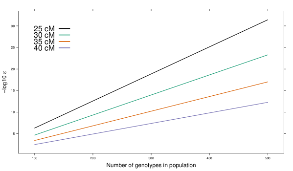
Figure 1: Negative log10 $\epsilon$ versus the number of genotypes in the population for four threshold cM distances.

2.2 Marker ordering

For simplicity, consider the $n\times t$ matrix of markers $\textstyle{M}$ belongs to the same linkage group. Preceding marker ordering, the markers are “binned” into groups where, within each group, the pairwise distance between any two markers is zero. The markers within each group have no recombinations between them and are said to be co-locating at the same genomic location for the $n$ genotypes used to construct the linkage map. A representative marker is then chosen from each of the bins and used to form the reduced $n\times t^{*}$ marker set ${\mathchoice{\hbox{\boldmath$\displaystyle{M}$}}{\hbox{\boldmath$\textstyle{M}$}}{\hbox{\boldmath$\scriptstyle{M}$}}{\hbox{\boldmath$\scriptscriptstyle{M}$}}}^{*}$.

For the reduced matrix ${\mathchoice{\hbox{\boldmath$\displaystyle{M}$}}{\hbox{\boldmath$\textstyle{M}$}}{\hbox{\boldmath$\scriptstyle{M}$}}{\hbox{\boldmath$\scriptscriptstyle{M}$}}}^{*}$, consider the complete set of entries $(j,k)\in(1,\ldots,t^{*})$ for either weight function (1) or (2). These complete set of entries can be viewed as the upper triangle of a symmetric weight matrix $\textstyle{W}$. MSTmap views all these entries as being connected edges in an undirected graph where the individual markers are vertices. A marker order for the set ${\mathchoice{\hbox{\boldmath$\displaystyle{M}$}}{\hbox{\boldmath$\textstyle{M}$}}{\hbox{\boldmath$\scriptstyle{M}$}}{\hbox{\boldmath$\scriptscriptstyle{M}$}}}^{*}$, also known as a travelling salesman path (TSP), is found by visiting each marker once and summing the weights from the connected edges. To find a minimum weight (TSP${}_{min}$), MSTmap uses a minimum spanning tree (MST) algorithm (ct76), such as Prims algorithm (prim57). If the TSP${}_{min}$ is unique then the MST is the optimal order for the markers. For cases where the data contains genotyping errors or lower numbers of individuals the MST may not be a complete path and contain markers or small sets of markers as individual nodes connected to the path. In these cases, MSTmap uses the longest path in the MST as the backbone and employs several efficient local optimization techniques such as K-opt, node-relocation and block-optimize (see mst08) to improve the current minimum TSP. By integrating these local optimization techniques into the algorithm, MSTmap provides users with a true one stage marker ordering algorithm.

A unique feature of the MSTmap algorithm is the use of an Expectation-Maximisation (EM) type algorithm for the imputation of missing allele scores that is tightly integrated with the ordering algorithm for the markers. To achieve this the marker matrix ${\mathchoice{\hbox{\boldmath$\displaystyle{M}$}}{\hbox{\boldmath$\textstyle{M}$}}{\hbox{\boldmath$\scriptstyle{M}$}}{\hbox{\boldmath$\scriptscriptstyle{M}$}}}^{*}$ is converted to a matrix, $\textstyle{A}$, where the entries represent the probabilistic certainty of the allele being AA. For the $j$th marker and $i$th individual then

$${\mathchoice{\hbox{\boldmath$\displaystyle{A}$}}{\hbox{\boldmath$\textstyle{A}$}}{\hbox{\boldmath$\scriptstyle{A}$}}{\hbox{\boldmath$\scriptscriptstyle{A}$}}}(i,j)=\left\{\begin{array}[]{ll}1&\quad\mbox{if ${\mathchoice{\hbox{\boldmath$\displaystyle{M}$}}{\hbox{\boldmath$\textstyle{M}$}}{\hbox{\boldmath$\scriptstyle{M}$}}{\hbox{\boldmath$\scriptscriptstyle{M}$}}}^{*}(i,j)$ is the A allele}\\ 0&\quad\mbox{if ${\mathchoice{\hbox{\boldmath$\displaystyle{M}$}}{\hbox{\boldmath$\textstyle{M}$}}{\hbox{\boldmath$\scriptstyle{M}$}}{\hbox{\boldmath$\scriptscriptstyle{M}$}}}^{*}(i,j)$ is the B allele}\\ {\mathchoice{\hbox{\boldmath$\displaystyle{R}$}}{\hbox{\boldmath$\textstyle{R}$}}{\hbox{\boldmath$\scriptstyle{R}$}}{\hbox{\boldmath$\scriptscriptstyle{R}$}}}_{j}/({\mathchoice{\hbox{\boldmath$\displaystyle{R}$}}{\hbox{\boldmath$\textstyle{R}$}}{\hbox{\boldmath$\scriptstyle{R}$}}{\hbox{\boldmath$\scriptscriptstyle{R}$}}}_{j}+{\mathchoice{\hbox{\boldmath$\displaystyle{S}$}}{\hbox{\boldmath$\textstyle{S}$}}{\hbox{\boldmath$\scriptstyle{S}$}}{\hbox{\boldmath$\scriptscriptstyle{S}$}}}_{j})&\quad\mbox{if ${\mathchoice{\hbox{\boldmath$\displaystyle{M}$}}{\hbox{\boldmath$\textstyle{M}$}}{\hbox{\boldmath$\scriptstyle{M}$}}{\hbox{\boldmath$\scriptscriptstyle{M}$}}}^{*}(i,j)$ is missing}\end{array}\right.$$ (7)

where ${\mathchoice{\hbox{\boldmath$\displaystyle{R}$}}{\hbox{\boldmath$\textstyle{R}$}}{\hbox{\boldmath$\scriptstyle{R}$}}{\hbox{\boldmath$\scriptscriptstyle{R}$}}}_{j}=(1-\hat{{\mathchoice{\hbox{\boldmath$\displaystyle{P}$}}{\hbox{\boldmath$\textstyle{P}$}}{\hbox{\boldmath$\scriptstyle{P}$}}{\hbox{\boldmath$\scriptscriptstyle{P}$}}}}_{j-1,j})(1-\hat{{\mathchoice{\hbox{\boldmath$\displaystyle{P}$}}{\hbox{\boldmath$\textstyle{P}$}}{\hbox{\boldmath$\scriptstyle{P}$}}{\hbox{\boldmath$\scriptscriptstyle{P}$}}}}_{j,j+1})$, ${\mathchoice{\hbox{\boldmath$\displaystyle{S}$}}{\hbox{\boldmath$\textstyle{S}$}}{\hbox{\boldmath$\scriptstyle{S}$}}{\hbox{\boldmath$\scriptscriptstyle{S}$}}}_{j}=\hat{{\mathchoice{\hbox{\boldmath$\displaystyle{P}$}}{\hbox{\boldmath$\textstyle{P}$}}{\hbox{\boldmath$\scriptstyle{P}$}}{\hbox{\boldmath$\scriptscriptstyle{P}$}}}}_{j-1,j}\hat{{\mathchoice{\hbox{\boldmath$\displaystyle{P}$}}{\hbox{\boldmath$\textstyle{P}$}}{\hbox{\boldmath$\scriptstyle{P}$}}{\hbox{\boldmath$\scriptscriptstyle{P}$}}}}_{j,j+1}$ and $\hat{{\mathchoice{\hbox{\boldmath$\displaystyle{P}$}}{\hbox{\boldmath$\textstyle{P}$}}{\hbox{\boldmath$\scriptstyle{P}$}}{\hbox{\boldmath$\scriptscriptstyle{P}$}}}}_{j,j-1},\hat{{\mathchoice{\hbox{\boldmath$\displaystyle{P}$}}{\hbox{\boldmath$\textstyle{P}$}}{\hbox{\boldmath$\scriptstyle{P}$}}{\hbox{\boldmath$\scriptscriptstyle{P}$}}}}_{j,j+1}$ are estimated recombination fractions between the $(j-1)$th and $j$th marker and $j$th and $(j+1)$th marker respectively. If ${\mathchoice{\hbox{\boldmath$\displaystyle{M}$}}{\hbox{\boldmath$\textstyle{M}$}}{\hbox{\boldmath$\scriptstyle{M}$}}{\hbox{\boldmath$\scriptscriptstyle{M}$}}}^{*}(i,j)$ is missing then the equation on the right hand side is the posterior probability of the missing value in marker $j$ being the A allele for genotype $i$ given the current estimate. Unlike the flanking marker methods of mc92; mc94 this equation represents a probabilistic approach to imputation. The ordering algorithm begins by initially calculating pairwise normalized distances between all markers in ${\mathchoice{\hbox{\boldmath$\displaystyle{M}$}}{\hbox{\boldmath$\textstyle{M}$}}{\hbox{\boldmath$\scriptstyle{M}$}}{\hbox{\boldmath$\scriptscriptstyle{M}$}}}^{*}$ and deriving an initial weight matrix, $\textstyle{W}$. An undirected graph is formed using the markers as vertices and the upper triangular entries of $\textstyle{W}$ as weights for the connected edges. An MST of the undirected graph is then found to establish an initial order for the markers of the linkage group. For the current order at the $(j-1,j,j+1)$th markers the E-step of algorithm requires updating the missing observation at marker $j$ by updating the estimates $\hat{{\mathchoice{\hbox{\boldmath$\displaystyle{P}$}}{\hbox{\boldmath$\textstyle{P}$}}{\hbox{\boldmath$\scriptstyle{P}$}}{\hbox{\boldmath$\scriptscriptstyle{P}$}}}}_{j-1,j}=\hat{d}_{j-1,j}/n$ and $\hat{{\mathchoice{\hbox{\boldmath$\displaystyle{P}$}}{\hbox{\boldmath$\textstyle{P}$}}{\hbox{\boldmath$\scriptstyle{P}$}}{\hbox{\boldmath$\scriptscriptstyle{P}$}}}}_{j,j+1}=\hat{d}_{j,j+1}/n$ in (7). The M-step then re-estimates the pairwise distances between all markers in ${\mathchoice{\hbox{\boldmath$\displaystyle{M}$}}{\hbox{\boldmath$\textstyle{M}$}}{\hbox{\boldmath$\scriptstyle{M}$}}{\hbox{\boldmath$\scriptscriptstyle{M}$}}}^{*}$ where, for the $j$th and $k$th marker, is

$$\hat{d}_{jk}=\sum_{i=1}^{t^{*}}{\mathchoice{\hbox{\boldmath$\displaystyle{A}$}}{\hbox{\boldmath$\textstyle{A}$}}{\hbox{\boldmath$\scriptstyle{A}$}}{\hbox{\boldmath$\scriptscriptstyle{A}$}}}(i,j)(1-{\mathchoice{\hbox{\boldmath$\displaystyle{A}$}}{\hbox{\boldmath$\textstyle{A}$}}{\hbox{\boldmath$\scriptstyle{A}$}}{\hbox{\boldmath$\scriptscriptstyle{A}$}}}(i,k))+{\mathchoice{\hbox{\boldmath$\displaystyle{A}$}}{\hbox{\boldmath$\textstyle{A}$}}{\hbox{\boldmath$\scriptstyle{A}$}}{\hbox{\boldmath$\scriptscriptstyle{A}$}}}(i,k)(1-{\mathchoice{\hbox{\boldmath$\displaystyle{A}$}}{\hbox{\boldmath$\textstyle{A}$}}{\hbox{\boldmath$\scriptstyle{A}$}}{\hbox{\boldmath$\scriptscriptstyle{A}$}}}(i,j))$$

and the weight matrix $\textstyle{W}$ is recalculated. An undirected graph is formed with the markers as vertices and the upper triangular entries of $\textstyle{W}$ as weights for the connected edges. A new order of the markers is derived by obtaining an MST of the undirected graph and the algorithm is repeated to convergence. Although this requires several iterations to converge, the computational time for the ordering algorithm remains efficient.

If required, the MSTmap algorithm also detects and removes genotyping errors as well as integrates this process into the ordering algorithm. The technique involves using a weighted average of nearby markers to determine the expected state of the allele. For individual $i$ and marker $j$ the expected value of the allele is calculated using

$$\mbox{E}[{\mathchoice{\hbox{\boldmath$\displaystyle{A}$}}{\hbox{\boldmath$\textstyle{A}$}}{\hbox{\boldmath$\scriptstyle{A}$}}{\hbox{\boldmath$\scriptscriptstyle{A}$}}}(i,j)]=\sum_{j\neq k}d_{j,k}^{-2}{\mathchoice{\hbox{\boldmath$\displaystyle{A}$}}{\hbox{\boldmath$\textstyle{A}$}}{\hbox{\boldmath$\scriptstyle{A}$}}{\hbox{\boldmath$\scriptscriptstyle{A}$}}}(i,k)\bigg{/}\sum_{j\neq k}d_{j,k}^{-2}$$

In this equation the weights are the inverse square of the distance from marker $j$ to its nearby markers. MSTmap only uses a small set of nearby markers during each iteration and the observed allele is considered suspicious if $|\mbox{E}[{\mathchoice{\hbox{\boldmath$\displaystyle{A}$}}{\hbox{\boldmath$\textstyle{A}$}}{\hbox{\boldmath$\scriptstyle{A}$}}{\hbox{\boldmath$\scriptscriptstyle{A}$}}}(i,j)]-{\mathchoice{\hbox{\boldmath$\displaystyle{A}$}}{\hbox{\boldmath$\textstyle{A}$}}{\hbox{\boldmath$\scriptstyle{A}$}}{\hbox{\boldmath$\scriptscriptstyle{A}$}}}(i,j)|>0.75$. If an observation is detected as suspicious it is treated as missing and imputed using the EM algorithm discussed previously. The removal of the suspicious allele has the effect of reducing the number of recombinations between the marker containing the suspicious observation and the neighbouring markers. This has an influential effect on the genetic distance between markers and the overall length of the linkage group.

The complete algorithm used to initially cluster the markers into linkage groups and optimally order markers within each linkage group, including imputing missing alleles and error detection, is known as the MSTmap algorithm.

2.3 Extension to RIL populations

The MSTmap algorithm can also be used to construct linkage maps for RIL populations generated through self-pollination of F1 derived individuals. These include inbred F2, F3, $\ldots$, F$r$ populations, where $r$ is the level or generation of selfing as well as Advanced RIL populations created by $r\rightarrow\infty$ levels of selfing. Non-advanced RIL populations contain three distinct genotypic states, two parental homozygotes (AA, BB) in equal proportions and a heterozygote (AB) with expected proportion determined by the simple decaying equation $2^{-(r-1)}$. As $r\rightarrow\infty$ this expected fraction tends to zero and the population can be considered to be an Advanced RIL containing parental (AA, BB) homozygotes only.

To ensure the MSTmap algorithm can be efficiently used to perform clustering and optimal ordering of markers for RIL populations, accurate estimates of pairwise recombination probabilities between markers are required. For an Advanced RIL the estimated recombination probability between any two markers ${\mathchoice{\hbox{\boldmath$\displaystyle{m}$}}{\hbox{\boldmath$\textstyle{m}$}}{\hbox{\boldmath$\scriptstyle{m}$}}{\hbox{\boldmath$\scriptscriptstyle{m}$}}}_{j}$ and ${\mathchoice{\hbox{\boldmath$\displaystyle{m}$}}{\hbox{\boldmath$\textstyle{m}$}}{\hbox{\boldmath$\scriptstyle{m}$}}{\hbox{\boldmath$\scriptscriptstyle{m}$}}}_{k}$, can be directly calculated using the result in bro05, namely

$$\hat{{\mathchoice{\hbox{\boldmath$\displaystyle{P}$}}{\hbox{\boldmath$\textstyle{P}$}}{\hbox{\boldmath$\scriptstyle{P}$}}{\hbox{\boldmath$\scriptscriptstyle{P}$}}}}^{*}_{jk}=(\hat{{\mathchoice{\hbox{\boldmath$\displaystyle{P}$}}{\hbox{\boldmath$\textstyle{P}$}}{\hbox{\boldmath$\scriptstyle{P}$}}{\hbox{\boldmath$\scriptscriptstyle{P}$}}}}_{jk}/2)/(1-\hat{{\mathchoice{\hbox{\boldmath$\displaystyle{P}$}}{\hbox{\boldmath$\textstyle{P}$}}{\hbox{\boldmath$\scriptstyle{P}$}}{\hbox{\boldmath$\scriptscriptstyle{P}$}}}}_{jk})$$ (8)

where $\hat{{\mathchoice{\hbox{\boldmath$\displaystyle{P}$}}{\hbox{\boldmath$\textstyle{P}$}}{\hbox{\boldmath$\scriptstyle{P}$}}{\hbox{\boldmath$\scriptscriptstyle{P}$}}}}_{jk}=d_{jk}/n$ is the estimated recombination probability between the two markers from a DH population. For any non-Advanced RIL, ${\mathchoice{\hbox{\boldmath$\displaystyle{P}$}}{\hbox{\boldmath$\textstyle{P}$}}{\hbox{\boldmath$\scriptstyle{P}$}}{\hbox{\boldmath$\scriptscriptstyle{P}$}}}_{jk}^{*}$ cannot be directly calculated and the MSTmap algorithm uses the recurrence relation results of hw31 (see Supplementary Text S1 mst08) and a simple stepwise optimization procedure to closely approximate ${\mathchoice{\hbox{\boldmath$\displaystyle{P}$}}{\hbox{\boldmath$\textstyle{P}$}}{\hbox{\boldmath$\scriptstyle{P}$}}{\hbox{\boldmath$\scriptscriptstyle{P}$}}}_{jk}^{*}$. Although Hoeffdings inequality (3) is well-defined for DH and BC populations, it is also used in the MSTmap algorithm to cluster markers for RIL populations. For large enough $r$, (8) can be approximately used to investigate the threshold p-value required for the inequality. At its theoretical boundaries, zero and 0.5, ${\mathchoice{\hbox{\boldmath$\displaystyle{P}$}}{\hbox{\boldmath$\textstyle{P}$}}{\hbox{\boldmath$\scriptstyle{P}$}}{\hbox{\boldmath$\scriptscriptstyle{P}$}}}_{jk}^{*}$ and ${\mathchoice{\hbox{\boldmath$\displaystyle{P}$}}{\hbox{\boldmath$\textstyle{P}$}}{\hbox{\boldmath$\scriptstyle{P}$}}{\hbox{\boldmath$\scriptscriptstyle{P}$}}}_{jk}$ are equivalent but for ${\mathchoice{\hbox{\boldmath$\displaystyle{P}$}}{\hbox{\boldmath$\textstyle{P}$}}{\hbox{\boldmath$\scriptstyle{P}$}}{\hbox{\boldmath$\scriptscriptstyle{P}$}}}_{jk}$ between $0.25$ and $0.35$, ${\mathchoice{\hbox{\boldmath$\displaystyle{P}$}}{\hbox{\boldmath$\textstyle{P}$}}{\hbox{\boldmath$\scriptstyle{P}$}}{\hbox{\boldmath$\scriptscriptstyle{P}$}}}_{jk}^{*}$ is substantially decreased creating a reduction of 10 cM+ in the genetic distance between the markers. Figure 1 indicates that this 10 cM reduction would require the p-value to be squared to achieve the appropriate threshold for clustering markers in RIL populations. Optimal ordering of markers within clustered linkage groups is then accomplished using the methods outlined in Section 2.2. However, for non-Advanced RIL populations only, the additional MSTmap algorithm features, including imputation of missing alleles scores and the detection of potential genotyping errors, have not been implemented.

3 ASMap package

3.1 Map construction functions

The ASMap package contains two linkage map construction functions that allow users to fully utilize the MSTmap parameters listed at http://alumni.cs.ucr.edu/~yonghui/mstmap.html and available for use with the source code.

mstmap.data.frame(object, pop.type = "DH", dist.fun = "kosambi", objective.fun = "COUNT", p.value = 1e-06, noMap.dist = 15, noMap.size = 0, miss.thresh = 1, mvest.bc = FALSE, detectBadData = FALSE, as.cross = TRUE, return.imputed = TRUE, trace = FALSE, …) The explicit form of the data frame object required for mstmap.data.frame() is borne from the syntax of the marker file required for using the MSTmap source code. It must have markers in rows and genotypes in columns. Marker names are required to be in the rownames component of the data frame, genotype names should reside in the names and each of the columns of the data frame must be of class "character" (not factors). The available populations that can be passed to the argument pop.type are "BC" Backcross, "DH" Doubled Haploid, "ARIL" Advanced Recombinant Inbred and "RILn" Recombinant Inbred with $n$ levels of selfing. It is recommended to set as.cross = TRUE to ensure the returned object can be used with the suite of ASMap and qtl package functions.

The second function provides greater linkage map construction flexibility by allowing users to pass an unconstructed or constructed "cross" object created from package qtl. mstmap.cross(object, chr, id = "Genotype", bychr = TRUE, suffix = "numeric", anchor = FALSE, dist.fun = "kosambi", objective.fun = "COUNT", p.value = 1e-06, noMap.dist = 15, noMap.size = 0, miss.thresh = 1, mvest.bc = FALSE, detectBadData = FALSE, return.imputed = FALSE, trace = FALSE, …) The object needs to inherit from one of the allowable classes available in the qtl package, namely "bc","dh","riself","bcsft" where "bc" is a Backcross "dh" is Doubled Haploid, "riself" is an advanced Recombinant Inbred (see ?convert2riself) and "bcsft" is a Backcross/Self (see ?convert2bcsft). The functions flexibility stems from the appropriate use of bychr and chr arguments. The logical flag bychr = FALSE ensures the the subset of linkage groups defined by chr will be bulked and reconstructed whereas bychr = TRUE confines the reconstruction within each linkage group defined by chr.

Users need to be aware the p.value argument available for both construction functions plays a crucial role in determining the clustering of markers to distinct linkage groups. Section 2.1 shows the separation of marker groups is highly dependent on the the number of individuals in the population. As a consequence, some trial and error may be required to determine an appropriate p.value for the linkage map being constructed. We have also provided an additional feature to the construction functions that allows the imputed probability matrix of representative markers to be returned if return.imputed = TRUE.

3.2 Pulling and pushing markers

Often in linkage map construction some pruning of the markers occurs before initial construction. For example, this may be the removal of markers with a proportion of missing values higher than some desired threshold as well as markers that are significantly distorted from their expected Mendelian segregation patterns. The removal is usually permanent and the possible importance of some of these markers may be overlooked. A preferable system would be to identify and place the problematic markers aside with the intention of checking their usefulness at a later stage of the construction process. The ASMap package contains two functions that allow you to do this. pullCross(object, chr, type = c("co.located","seg.distortion","missing"), pars = NULL, replace = FALSE, …) pushCross(object, chr, type = c("co.located","seg.distortion","missing", "unlinked"), unlinked.chr = NULL, pars = NULL, replace = FALSE, …) The construction helper functions share three types of markers that can be “pulled/pushed” from linkage maps. These include markers that are co-located with other markers, markers that have some defined segregation distortion and markers with a defined proportion of missing values. If the argument type is "seg.distortion" or "missing" then the initialization function pp.init() pp.init(seg.thresh = 0.05, seg.ratio = NULL, miss.thresh = 0.1, max.rf = 0.25, min.lod = 3) is used to determine the appropriate threshold parameter setting (seg.thresh, seg.ratio, miss.thresh) that will be used to pull/push markers from the linkage map. Users can set their own parameters by appropriate use of the pars argument. For each different type, pullCross() will pull markers from the map and place them in separate elements of the returned object. Within the elements, vital information is kept that can be accessed by pushCross() to push the markers back at a later stage of linkage map construction. The function pushCross() also contains another marker type called "unlinked" which, in conjunction with the argument unlinked.chr, allows users to push markers from an unlinked linkage group in the geno element of the object into established linkage groups. This mechanism becomes vital, for example, when pushing new markers into an established linkage map.

3.3 Visual diagnostics

To provide a complete system for efficient linkage map construction ASMap contains graphical functions for visuals diagnosis of your constructed linkage map. Three flexible functions are provided and examples of their use are given in Section 4.

profileGen(cross, chr, bychr = TRUE, stat.type = c("xo", "dxo", "miss"), id = "Genotype", xo.lambda = NULL, …) The function profileGen() calls statGen() to obtain statistics for graphically profiling information about the genotypes across the marker set and also returns the statistics invisibly after plotting. The current statistics that can be calculated and profiled include

• "xo" : number of crossovers.

• "dxo" : number of double crossovers.

• "miss" : number of missing values.

The two statistics "xo" and "dxo" are only useful for constructed linkage maps. From the authors experience, they represent the most vital two statistics for determining a linkage maps quality. Inflated crossover or double crossover rates of any genotypes indicate problematic lines and should be questioned. Significant crossover rates can be checked by manually inputting a median crossover rate using the argument xo.lambda. Additional graphical parameters can be passed to the high level lattice function xyplot() through the "…" argument profileMark(cross, chr, stat.type = "marker", use.dist = TRUE, map.function = "kosambi", crit.val = NULL, display.markers = FALSE, mark.line = FALSE, …) The function profileMark() calls statMark() and graphically profiles marker/interval statistics as well as returns them invisibly after plotting. The current marker statistics that can be profiled are

• "seg.dist": -log10 p-value from a test of segregation distortion.

• "miss": proportion of missing values.

• "prop": allele proportions.

• "dxo": number of double crossovers.

The current interval statistics that can be profiled are

• "erf": estimated recombination fractions.

• "lod": LOD score for the test of no linkage.

• "dist": interval map distance.

• "mrf": map recombination fraction.

• "recomb": number of recombinations.

The function allows any combination of marker/interval statistics to be plotted simultaneously on a multi-panel lattice display. There is a chr argument to subset the linkage map to user defined linkage groups. If crit.val = "bonf" then markers that have significant segregation distortion greater than the family wide alpha level of $0.05/m$, where $m$ is the number of markers, will be annotated in marker panels. Similarly, intervals that have a significantly weak linkage from a test of the recombination fraction of $r=0.5$ will also be annotated in the interval panels. All linkage groups are highlighted in a different colours to ensure they can be identified clearly. The lattice panels ensure that marker and interval statistics are seamlessly plotted together so problematic regions or markers can be identified efficiently. Additional graphical parameters can be passed to xyplot() through the "…" argument.

heatMap(x, chr, mark, what = c("both", "lod", "rf"), lmax = 12, rmin = 0, markDiagonal = FALSE, color = rev(colorRampPalette(brewer.pal(11, "Spectral"))(256)), …) ASMap contains an improved version of the heat map that rectifies limitations of the heat map, plot.rf(), available in qtl. The function independently plots the LOD score on the bottom triangle of the heat map as well as the actual estimated recombination fractions (RFs) on the upper triangle. A colour key legend is also provided for the RFs and LOD scores on the left and right hand side of the heat map respectively. As the actual estimated RFs are plotted, the scale of the legend includes values beyond the theoretical threshold of 0.5. By increasing this scale beyond 0.5, potential regions where markers out of phase with other markers can be recognised. Similar to plot.rf(), the heatMap() function allows subsetting of the linkage map by chr and users can further subset the linkage groups using the argument mark by indexing a set of markers within linkage groups defined by chr.

3.4 Miscellaneous functions

In the authors experience, the assumptions of how the individuals of a population are genetically related is rarely checked throughout the construction process. Too often unconstructed or constructed linkage maps contain individuals that are closely related beyond the simple assumptions of the population. ASMap contains a function for the detection and reporting of the relatedness between individuals as well as a function for forming consensus genotypes if genuine clones are found. genClones(object, chr, tol = 0.9, id = "Genotype") fixClones(object, gc, id = "Genotype", consensus = TRUE) The genClones() function uses the power of comparegeno() from the qtl package to perform the relatedness calculations. It then provides a numerical breakdown of the relatedness between pairs of individuals that share a proportion of alleles greater than tol. This breakdown also includes the clonal group the pairs of individuals belong to. The table of information from this calculation can then be passed to fixClones() through the argument gc and consensus genotypes are formed through the appropriate merging of alleles across genotypes within clone groups.

During the linkage map construction process there may be a requirement to break or merge linkage groups. ASMap provides two functions to achieve this. breakCross(cross, split = NULL, suffix = "numeric", sep = ".") mergeCross(cross, merge = NULL, gap = 5) The breakCross() function allows users to break linkage groups in a variety ways. The split argument takes a list with elements named by the linkage group names that require splitting and containing the markers that immediately proceed where the splits are to be made. The mergeCross() function provides a method for merging linkage groups. Its argument merge requires a list with elements named by the proposed linkage group names required and containing the linkage groups to be merged. It should be noted that this function places an artificial genetic distance gap between the merged linkage groups. Accurate distance estimation would require a separate map estimation procedure after merging has taken place.

In qtl genetic distances can be estimated using est.map() or through read.cross() when setting the argument estimate.map = TRUE. The estimation uses the multi-locus hidden Markov model technology of lg87. Unfortunately this is computationally cumbersome if there are many markers on a linkage group and becomes more so if there are many missing allele calls and genotyping errors present. ASMap contains a small map estimation function that circumvents this computational burden. quickEst(object, chr, map.function = "kosambi", …) The quickest() function makes use of another function in qtl called argmax.geno(). This function is also a multi-locus hidden Markov algorithm that uses the observed markers present in a linkage group to impute pseudo-markers at any chosen cM genetic distance. In this case, the requirement is for a reconstruction or imputation at the markers themselves. For the most accurate imputation to occur there needs to be an estimate of genetic distance in place and this is calculated by converting recombination fractions to genetic distances after calling est.rf(). As a result, the quickEst() function lives up to its namesake by providing efficient and accurate genetic distance calculations for large linkage maps.

The functions pullCross() and pushCross() described in Section 3.2 are used to create and manipulate extra list elements "co.located", "seg.distortion" and "missing" associated with different marker types. Unfortunately, these list elements are not recognized by the native qtl functions. If the function subset.cross() is used to subset the object to a reduced number of individuals then the data component of each of these elements will not be subsetted accordingly. In addition, the statistics in the table component of the elements "seg.distortion" and "missing" will be incorrect for the newly subsetted linkage map. subsetCross(cross, chr, ind, …) This subset function contains identical functionality to subset.cross() but also ensures the data components of the extra list elements "co.located", "seg.distortion" and "missing" are subsetted to match the linkage map. In addition, for elements "seg.distortion" and "missing" it also updates the table components to reflect the newly subsetted map, ensuring pushCross() uses the most accurate information when determining which markers to push back into the linkage map.

There is often a requirement to incorporate additional markers to an established linkage map or merge two linkage maps from the same population. This idea motivated the creation of the combineMap() ASMap package. The aim of the function was to merge linkage maps based on shared map information, readying the combined linkage groups for reconstruction through an efficient linkage map construction process such as mstmap.cross(). combineMap(…, id = "Genotype", keep.all = TRUE) The function takes an unlimited number of linkage maps through the … argument. The linkage maps must all have the same cross class structure and contain the same genotype identifier id. The merging of the maps happens intelligently with initial merging based on commonality between the genotypes. If keep.all = TRUE the new combined linkage map is “padded out” with missing values where genotypes are not shared. If keep.all= FALSE the combined map is reduced to genotypes that are shared among all linkage maps. Secondly, if linkage group names are shared between maps then the markers from common linkage groups are clustered.

4 Illustrative example

To showcase the functionality of the ASMap package, the complete linkage map construction process is presented for a barley Backcross population containing 3024 markers genotyped on 326 individuals in an unconstructed marker set formatted as a qtl object with class "bc". The data is available in the ASMap package using R> library("ASMap") R> data("mapBCu")

4.1 Pre-construction

Before constructing a linkage map it is prudent to go through a pre-construction checklist to ensure that the best quality genotypes/markers are being used to construct the linkage map. A non-exhaustive ordered checklist for an unconstructed marker set could be

• Check missing allele scores across markers for each genotype as well as across genotypes for each marker. Markers or genotypes with a high proportion of missing information could be problematic.

• Check for genetic clones or individuals that have a high proportion of matching allelic information between them.

• Check markers for excessive segregation distortion. Highly distorted markers may not map to unique locations.

• Check markers for switched alleles. These markers will not cluster or link well with other markers during the construction process and it is therefore preferred to repair their alignment before proceeding.

• Check for co-locating markers. For large linkage maps it would be more computationally efficient from a construction standpoint to temporarily omit markers that are co-located with other markers.

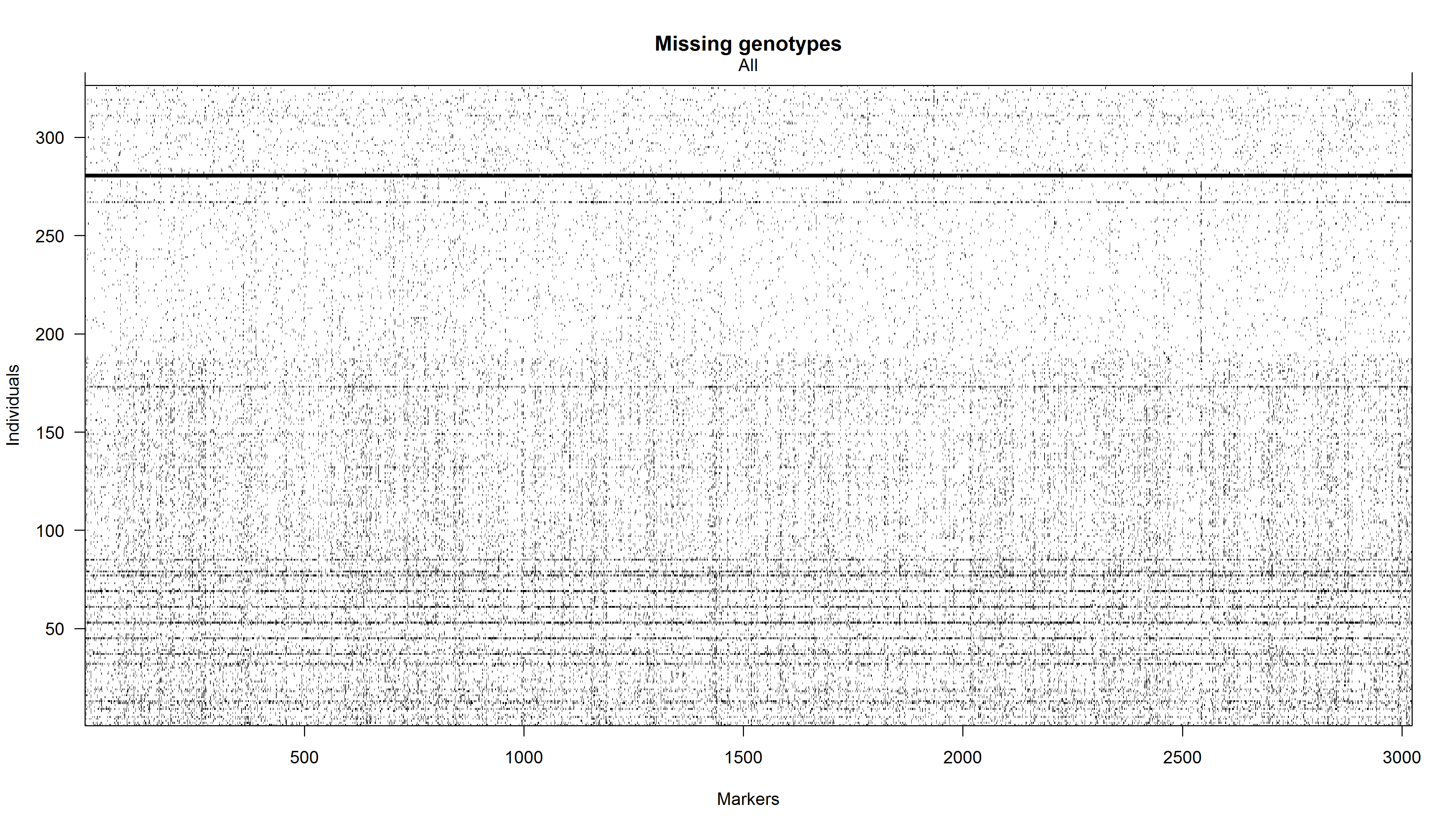
Figure 2: Plot of the missing allele scores for the unconstructed map mapBCu.

Figure 2 shows the result of a call to the missing value diagnostic plot plot.missing() available in qtl. R> plot.missing(mapBCu) The darkest horizontal lines on the plot indicate there are some genotypes with large amounts of missing data. This could indicate poor physical genotyping of these lines and should be removed before proceeding. The plot also reveals the markers have a large number of typed allele values across the range of genotypes. The ASMap function statGen() was used to identify genotypes with more than 50% missing alleles across the markers. These were omitted using the usual functions available in qtl. R> sg <- statGen(mapBCu, bychr = FALSE, stat.type = "miss") R> mapBC1 <- subset(mapBCu, ind = sg$miss<1600)Fromamapconstructionpointofview,highlyrelatedindividualsmayenhancesegregationdistortionofmarkers.Itisthereforewisetodetermineacourseofactionsuchasremovalofindividualsorthecreationofconsensusgenotypesbeforeproceedingwithanyfurtherpre-constructiondiagnostics.The\pkg{ASMap}function\code{genClones()}discussedinSection\ref{sec:misc}wasusedtoidentifyandreportgeneticclones.\Schunk\Sinput R>gc<-genClones(mapBC1,tol=0.95)R>gc$cgd\Soutput G1G2coefmatchdiffna.bothna.onegroup1BC045BC0390.991914661297144812BC052BC0391.0000242309850213BC168BC0391.0000257204740414BC052BC0450.989914761594143815BC168BC0450.987216202144133816BC168BC0521.0000257703641017BC067BC0601.000027590825628BC135BC0861.0000274301726339BC099BC0931.00002737019267410BC120BC1171.00002699022302511BC129BC1261.00002678035310612BC204BC1381.0000269106326713BC147BC1410.99962753122247814BC193BC1441.0000277107245915BC162BC1611.000026860203171016BC205BC1901.00002886071301117BC286BC2851.00002920011021218BC325BC3141.000029110410813Thetableshows13groupsofgenotypesthatshareaproportionoftheirallelesgreaterthan0.95.Thesuppliedadditionalstatisticsshowthatthefirstgroupcontainsthreepairsofgenotypesthathadmatchedpairsofallelesfrom1620markersorless.Thesepairsalsohad$∼1400$markerswhereanallelewaspresentforonegenotypeandmissingforanother.Basedonthis,therewasnotenoughevidencetosuspectthesepairsmaybeclonesandtheywereremovedfromthetable.ThefixClones()functionwasthenbeusedtoformconsensusgenotypesfortheremaininggroupsofclonesinthetable.R>cgd<-gccgd[-c(1,4,5),]R>mapBC2<-fixClones(mapBC1,cgd,consensus=TRUE)Atthisjunctureitiswisetocheckwhethertheobservedallelicfrequenciesataspecificlocideviatefromexpectedallelicfrequencies.Thisiscalledsegregationdistortionanditiswellknowntooccurfromerrorsinthephysicallaboratorialprocessesandcanalsooccurinlocalgenomicregionsfromunderlyingbiologicalandgeneticmechanisms\text{<cite class="ltx\_cite ltx\_citemacro\_citep">(<span class="ltx\_ref ltx\_missing\_citation ltx\_ref\_self">lytt91</span>)</cite>}.Thesignificanceofthesegregationdistortion,theallelicproportionsandthemissingvalueproportionacrossthegenomecanbegraphicallyrepresentedusingthemarkerprofilingfunctionprofileMark()andtheresultisdisplayedinFigure\text{<span class="ltx\_ref ltx\_missing\_label ltx\_font\_italic ltx\_ref\_self">LABEL:fig:seg1</span>}.R>profileMark(mapBC2,stat.type=c(\mathrm{"}seg.dist\mathrm{"},\mathrm{"}prop\mathrm{"},\mathrm{"}miss\mathrm{"}),crit.val=+\mathrm{"}bonf\mathrm{"},layout=c(1,4),type=\mathrm{"}l\mathrm{"})Settingcrit.val=\mathrm{"}bonf\mathrm{"}annotatesthemarkersineachpanelthathaveap-valueforthetestofsegregationdistortionlowerthanthefamilywidebonferroniadjustedalphalevelof0.05/(totalnumberofmarkers).Theplotindicatestherearenumerousmarkersthataresignificantlydistortedwiththreehighlydistortedmarkers.Theplotalsoshowsthemissingvalueproportionofthemarkersdoesnotexceed20\%.\text{Figure 3Figure 33Figure 33Forindividualmarkers,thenegativelog10p-valueforthetestofsegregat}$