Smooth positon solutions of the focusing modified Korteweg-de Vries equation

Abstract

The $n$-fold Darboux transformation $T_{n}$ of the focusing real modified Korteweg-de Vries (mKdV) equation is expressed in terms of the determinant representation. Using this representation, the $n$-soliton solutions of the mKdV equation are also expressed by determinants whose elements consist of the eigenvalues $\lambda_{j}$ and the corresponding eigenfunctions of the associated Lax equation. The nonsingular $n$-positon solutions of the focusing mKdV equation are obtained in the special limit $\lambda_{j}\rightarrow\lambda_{1}$, from the corresponding $n$-soliton solutions and by using the associated higher-order Taylor expansion. Furthermore, the decomposition method of the $n$-positon solution into $n$ single-soliton solutions, the trajectories, and the corresponding “phase shifts” of the multi-positons are also investigated.

1 Introduction

It is a well-known fact that nonlinear partial differential equations play a fundamental role both in the understanding of many natural phenomena and in the development of advanced technologies and engineering designs. A plethora of such nonlinear evolutions equations have been investigated during the many years such as the celebrated Korteweg-de Vries (KdV) equation, the modified Korteweg-de Vries (mKdV) equation, the sine-Gordon (sG) equation, the nonlinear Schrödinger (NLS) equation, the Manakov system, Kadomtsev-Petviashvili equation, Davey-Stewartson equation, Maccari system etc. Especially, the origin of the KdV equation and its birth has been a long process and spanned a period of about sixty years from the experiments of Scott-Russell in 1834 su-1 to the publication in 1895 of a seminal article by Korteweg and de Vries NK who developed a mathematical model for the shallow water problem and demonstrated the possibility of solitary wave generation. The KdV equation has been derived in a series of physical settings, e.g. in plasma physics E-2 ; E-1 , and in studies of anharmonic (nonlinear) lattices o-3 ; o-4 . Here we recall that the existence and uniqueness of solutions of the KdV equation for appropriate initial and boundary conditions have been proved by Sjöberg o-5 . It is well known that if $u$ is a solution of the KdV equation $u_{t}+u_{xxx}-6uu_{x}=0$ and $v$ is a solution of the defocusing mKdV equation $v_{t}+v_{xxx}-6v^{2}v_{x}=0$, the two solutions are connected by the Miura transformation AK1 , namely, $u=v_{x}+v^{2}$. Both KdV and mKdV equations are completely integrable and have infinitely many conserved quantities AK2 .

The KdV and mKdV equations and its many generalizations were used to describe a series of physical phenomena. For example, the system of coupled KdV equations is a generic model of resonantly coupled internal waves in stratified fluids and can also describe the formation of gap solitons and of parametric envelope solitons, see Ref. B1 -B5 . In optical settings the mKdV equation and its further generalizations were found to adequately describe the propagation in nonlinear optical media of ultrasort pulses consisting of only a few optical cycles, beyond the so-called slowly varying envelope aproximation LM2009 -M2015 . Recently, a model based on two coupled mKdV equations was used to describe the soliton propagation in two parallel optical waveguides, in the presence of linear nondispersing coupling and in the few-cycle regime Terniche2016 . The mKdV, sG, and mKdV-sG equations were used in modelling the process of generation of supercontinuum light in optical fibers SCG2014 ; SCG2016 . The mKdV equation also appears in other fields such as ion acoustic soliton experiments in plasmas YOC1 ; ion1 , fluid mechanics RW1 , soliton propagation in lattices and acoustic waves in certain anharmonic lattices H1 , nonlinear van Alfvén waves propagating in plasmas H2 ; H22 , meandering ocean currents H3 , the dynamics of traffic flow on ; Y.11 , and the study of Schottky barrier transmission lines Y.12 . For a series of recent studies of the KdV and mKdV equations, and other relevant nonlinear partial differential equations that describe the dynamics of diverse physical phenomena, see Refs. Ra -Rk . It is worth mentioning that being a completely integrable nonlinear dynamical system, the generic mKdV partial differential equation possesses unique features such as the Painlevé property property1 ; property11 , Miura transformation property2 , the inverse scattering transformation property3 , the Darboux transformation (DT)YO-6 and so on.

In a pioneering work kdv1992 , Matveev introduced the concept of a positon solution as a new type of solution of the KdV equation. Both positon and soliton-positon solutions of the KdV equation were first constructed and analyzed kdv1992 . The positon solutions have many interesting properties that differ from those of soliton solutions. The positons can be characterized as slowly decaying oscillating solutions of the nonlinear completely integrable equations having the special property of being superreflectionless HE2 . The positons are weakly localized, in contrast to exponentially decaying soliton solutions. For a positon solution the corresponding eigenvalue of the spectral problem is positive and is embedded in the continuous spectrum. The positons are completely transparent to other interacting objects. In particular, two positons remain unchanged after mutual collision. However, during the soliton-positon collision the soliton remains unchanged, while both the carrier-wave of the positon and its envelope experience finite phase-shifts HE3 ; onorato . The positon solutions were then constructed for many other models, such as the defocusing mKdV equation positon1992 ; positon1995 , the sG equation Y.Ohta12 and the Toda-lattice YOC . It is well known that that the above mentioned positon solutions are singular ones. So it is important from the point of view of possible applications of positon solutions to model diverse physical phenomena to seek smooth, nonsingular positon solutions for nonlinear evolution equations. It is worth noting that it is not possible to get smooth, nonsingular positon solutions of the defocusing mKdV because of the singularity that is inherent in its Darboux transformation. Instead, it is natural to seek nonsingular positon solutions of the following focusing-type mKdV equation

$$q_{t}=\frac{q_{xxx}}{4}+\frac{3q^{2}q_{x}}{2}$$ (1)

by using the DT method. Here $q=q(x,t)$ is a real function of variables $x$ and $t$. Furthermore, we know that the multi-soliton solution for the mKdV equation has been given, e.g., in Refs. dubardthesis2010 ; matveev2011nlsKPI ; Gaillard-2011-435204 . We should note that the $n$-soliton solution of the mKdV equation can be decomposed into a summation of $n$ single solitons with a constant phase shift at $|t|\longrightarrow\infty$, see, for example Ref. matveev2011nlsKPI . It is the main aim of this paper to decompose the multi-positon solution of the focusing real mKdV equation, and to further study its key properties of the nonsigular positons including their trajectories and the associated “phase shift”.

The organization of this paper is as follows. In Section 2, the $n$-fold Darboux transformation is given. In Section 3, the positon solution of the focusing real mKdV equation is calculated by using the degenerate Darboux transformation method and a special Taylor expansion. The multi-positon solution and its decomposition into several single-positon solutions, the associated positon trajectories and phase shifts are also discussed. Our conclusions are provided in the last section.

2 The Darboux transformation of the focusing mKdV equation

The Lax pair of the mKdV equation (1) can be derived by the Lie algebra splitting AKNS ; DS84 ; TUa ; TUb :

$$\phi_{x}{(\lambda)}=M\phi{(\lambda)},$$ (2)

$$\phi_{t}{(\lambda)}=(N_{3}{\lambda}^{3}+N_{2}{\lambda}^{2}+N_{1}{\lambda}+N_{0})\phi{(\lambda)}=N\phi{(\lambda)},$$ (3)

with

$${\phi(\lambda)}=\left[\begin{array}[]{ccc}\varphi_{1}(\lambda)\\ \varphi_{2}(\lambda)\end{array}\right],\qquad\qquad{M}=\left[\begin{array}[]{ccc}\lambda&q\\ -q&-\lambda\end{array}\right],\qquad\qquad{N_{3}}=\left[\begin{array}[]{ccc}1&0\\ 0&-1\end{array}\right],$$

$${N_{2}}=\left[\begin{array}[]{ccc}0&q\\ -q&0\end{array}\right],\qquad{N_{1}}=\left[\begin{array}[]{ccc}\frac{q^{2}}{2}&\frac{q_{x}}{2}\\ \frac{q_{x}}{2}&-\frac{q^{2}}{2}\end{array}\right],\qquad{N_{0}}=\left[\begin{array}[]{ccc}0&\frac{q_{xx}+2q^{3}}{4}\\ \frac{-q_{xx}-2q^{3}}{4}&0\end{array}\right].$$

Here $\phi(\lambda)$ is an eigenfunction of the Lax equation associated with eigenvalue $\lambda$. In order to later construct the kernel of $n$-fold DT, it is necessary to introduce 2n eigenfunctions:

$$\phi_{2j-1}=\phi{(\lambda)}|_{\lambda=\lambda_{2j-1}}=\left[\begin{array}[]{c}\phi_{2j-1,1}\\ \phi_{2j-1,2}\\ \end{array}\right]\quad\phi_{2j}=\phi{(\lambda)}|_{\lambda=\lambda_{2j}}=\left[\begin{array}[]{c}\phi_{2j,1}\\ \phi_{2j,2}\\ \end{array}\right].$$

The even-numbered functions are given through the reduction condition:

$$\lambda_{2j}=-\lambda_{2j-1},\quad\phi_{2j}=\left[\begin{array}[]{cc}\phi_{2j,1}\\ \phi_{2j,2}\end{array}\right]=\left[\begin{array}[]{c}-\phi_{2j-1,2}\\ \phi_{2j-1,1}\end{array}\right].$$ (4)

Here $\varphi_{1}(x,t,\lambda)$ and $\varphi_{2}(x,t,\lambda)$ are the two components of eigenfunction $\phi$ associated with $\lambda$ in Eqs. (2) and (3). Furthermore, we will set $T$ to be a gauge transformation as follows

$$\phi^{[1]}=T\phi,~{}~{}q\rightarrow q^{[1]},$$ (5)

$$\phi_{x}^{[1]}=M^{[1]}\phi^{[1]},$$ (6)

$$\phi_{t}^{[1]}=N^{[1]}\phi^{[1]}.$$ (7)

According to Eqs. (2), (3), (5), (6), and (7), it is easy to get

$$M^{[1]}T=T_{x}+TM.$$ (8)

Similarly, the following equation can be also obtained

$$N^{[1]}T=T_{t}+TN.$$ (9)

Hence, we get

$$M_{t}^{[1]}-N_{x}^{[1]}+[M^{[1]},N^{[1]}]=0.$$ (10)

In general, in order to seek for Darboux transformation, we assume

$${T}=\left[\begin{array}[]{ccc}a_{1}&b_{1}\\ c_{1}&d_{1}\end{array}\right]\lambda+\left[\begin{array}[]{ccc}a_{0}&b_{0}\\ c_{0}&d_{0}\end{array}\right].$$ (11)

Here, $a_{0},b_{0},c_{0},d_{0},a_{1},b_{1},c_{1}$, and $d_{1}$ are functions of $x$ and $t$, which can be easily obtained according to the Eqs. (9) and (10), by comparing the coefficients of $\lambda^{i}\,(i=4,3,2,1,0)$.

For example, it is easily to get $a_{1t}=0,\quad b_{1t}=0$, by comparing the coefficients of $\lambda$. Furthermore, $a_{1x}=0,\quad b_{1x}=0,$ so $a_{1}$ and $d_{1}$ are arbitrary constants. Then we set $a_{1}=1$,  $b_{1}=1$ in order to simplify the later calculations without loss of generality, i.e.,

$${T_{1}}=\left[\begin{array}[]{ccc}1&0\\ 0&1\end{array}\right]\lambda+\left[\begin{array}[]{ccc}a_{0}&b_{0}\\ c_{0}&d_{0}\end{array}\right].$$ (12)

Then, $a_{0}$,  $b_{0}$, $c_{0}$, and  $d_{0}$ can be obtained by using the kernel of $T_{1}$:

$$T_{1}(\lambda;\lambda_{1},\lambda_{2})\phi{(\lambda)}|_{\lambda=\lambda_{1}}=0,\quad T_{1}(\lambda;\lambda_{1},\lambda_{2})\phi{(\lambda)}|_{\lambda=\lambda_{2}}=0.$$

Here the two eigenfunctions $\phi{(\lambda_{1})}$ and $\phi{(\lambda_{2})}$ are in the form of

$$\phi(\lambda_{1})=\left[\begin{array}[]{ccc}\phi_{11}\\ \phi_{12}\end{array}\right],\qquad\phi(\lambda_{2})=\left[\begin{array}[]{ccc}\phi_{21}\\ \phi_{22}\end{array}\right].$$

Solving the above algebraic equations, then

$${a_{0}}=-\frac{\left|\begin{array}[]{ccc}\lambda_{1}\phi_{11}&\phi_{12}\\ \lambda_{2}\phi_{21}&\phi_{22}\end{array}\right|}{|W_{2}|},\qquad{b_{0}}=\frac{\left|\begin{array}[]{ccc}\lambda_{1}\phi_{11}&\phi_{11}\\ \lambda_{2}\phi_{21}&\phi_{21}\end{array}\right|}{|W_{2}|},$$

$${c_{0}}=\frac{\left|\begin{array}[]{ccc}\phi_{12}&\lambda_{1}\phi_{12}\\ \phi_{22}&\lambda_{2}\phi_{21}\end{array}\right|}{|W_{2}|},\qquad{d_{0}}=-\frac{\left|\begin{array}[]{ccc}\phi_{11}&\lambda_{1}\phi_{12}\\ \phi_{21}&\lambda_{2}\phi_{22}\end{array}\right|}{|W_{2}|}.$$

Taking these elements back into $T_{1}$, then the determinant representation of $T_{1}$ is given by

$${T_{1}}=\frac{1}{|W_{2}|}{\left|\begin{array}[]{ccccc}(\widetilde{T_{1}})_{11}&(\widetilde{T_{1}})_{12}\\ (\widetilde{T_{1}})_{21}&(\widetilde{T_{1}})_{22}\end{array}\right|},\qquad\qquad{W_{2}}=\left[\begin{array}[]{ccc}\phi_{11}&\phi_{12}\\ \phi_{21}&\phi_{22}\end{array}\right],$$ (13)

$${(\widetilde{T_{1}})_{11}}=\frac{\left|\begin{array}[]{ccccc}1&0&\lambda\\ \phi_{11}&\phi_{12}&\lambda_{1}\phi_{11}\\ \phi_{21}&\phi_{22}&\lambda_{2}\phi_{21}\end{array}\right|}{|W_{2}|},\qquad{(\widetilde{T_{1}})_{12}}=\frac{\left|\begin{array}[]{ccccc}0&1&0\\ \phi_{11}&\phi_{12}&\lambda_{1}\phi_{11}\\ \phi_{21}&\phi_{22}&\lambda_{2}\phi_{21}\end{array}\right|}{|W_{2}|},$$

$${(\widetilde{T_{1}})_{21}}=\frac{\left|\begin{array}[]{ccccc}1&0&\lambda\\ \phi_{11}&\phi_{12}&\lambda_{1}\phi_{11}\\ \phi_{21}&\phi_{22}&\lambda_{2}\phi_{21}\end{array}\right|}{|W_{2}|},\qquad{(\widetilde{T_{1}})_{22}}=\frac{\left|\begin{array}[]{ccccc}0&1&0\\ \phi_{11}&\phi_{12}&\lambda_{1}\phi_{11}\\ \phi_{21}&\phi_{22}&\lambda_{2}\phi_{21}\end{array}\right|}{|W_{2}|}.$$

Further, the one-fold Darboux transformation $T_{1}$ generates a new solution of the focusing mKdV equation

$${q^{[1]}}=q+\frac{2}{|W_{2}|}{\left|\begin{array}[]{ccc}\phi_{11}&\lambda_{1}\phi_{11}\\ \phi_{21}&\lambda_{2}\phi_{21}\end{array}\right|},$$ (14)

according to Eq. (8). Note that $\phi_{2}$ and $\lambda_{2}$ are given by the reduction condition in Eq. (4)

By iterating $n$ times $T_{1}$ and using the representation of $T_{1}$, it is easy to get the $n$-fold Darboux transformation, see the following theorem.
Theorem The $n$-fold Darboux transformation of the mKdV equation (1) is as follows

$${T_{n}}=T_{n}(\lambda)=\frac{\left|\begin{array}[]{ccccc}(\widetilde{T_{n}})_{11}&(\widetilde{T_{n}})_{12}\\ (\widetilde{T_{n}})_{21}&(\widetilde{T_{n}})_{22}\end{array}\right|}{|W_{2n}|},$$ (15)

where

$${W_{2n}}=\left[\begin{array}[]{ccccccc}\phi_{11}&\phi_{12}&\lambda_{1}\phi_{11}&\lambda_{1}\phi_{12}&\cdots\lambda_{1}^{n-1}\phi_{11}&\lambda_{1}^{n-1}\phi_{12}\\ \phi_{21}&\phi_{22}&\lambda_{2}\phi_{21}&\lambda_{2}\phi_{22}&\cdots\lambda_{2}^{n-1}\phi_{11}&\lambda_{2}^{n-1}\phi_{12}\\ \phi_{31}&\phi_{32}&\lambda_{3}\phi_{31}&\lambda_{3}\phi_{32}&\cdots\lambda_{3}^{n-1}\phi_{11}&\lambda_{3}^{n-1}\phi_{12}\\ \vdots&\vdots&\vdots&\vdots&\vdots&\vdots\\ \phi_{2n,1}&\phi_{2n,2}&\lambda_{2n}\phi_{2n,1}&\lambda_{2n}\phi_{2n,2}&\lambda_{2n}^{n-1}\phi_{2n,1}&\lambda_{2n}^{n-1}\phi_{2n,2}\end{array}\right],$$

$$\mbox{}\mathbf{(\widetilde{T_{n}})_{11}}=\frac{\left|\begin{array}[]{cccccccccc}1&0&\lambda&0&\lambda^{2}&0&\cdots\lambda^{n-1}&0&\lambda^{n}\\ \phi_{11}&\phi_{12}&\lambda_{1}\phi_{11}&\lambda_{1}\phi_{12}&\lambda_{1}^{2}\phi_{11}&\lambda_{1}^{2}\phi_{12}&\cdots\lambda_{1}^{n-1}\phi_{11}&\lambda_{1}^{n-1}\phi_{12}&\lambda_{1}^{n}\phi_{11}\\ \phi_{21}&\phi_{22}&\lambda_{2}\phi_{21}&\lambda_{2}\phi_{22}&\lambda_{2}^{2}\phi_{21}&\lambda_{2}^{2}\phi_{22}&\cdots\lambda_{2}^{n-1}\phi_{21}&\lambda_{2}^{n-1}\phi_{22}&\lambda_{2}^{n}\phi_{21}\\ \phi_{31}&\phi_{32}&\lambda_{3}\phi_{31}&\lambda_{3}\phi_{32}&\lambda_{3}^{2}\phi_{31}&\lambda_{3}^{2}\phi_{32}&\cdots\lambda_{3}^{n-1}\phi_{31}&\lambda_{3}^{n-1}\phi_{32}&\lambda_{3}^{n}\phi_{31}\\ \vdots&\vdots&\vdots&\vdots&\vdots&\vdots&\vdots&\vdots&\vdots\\ \phi_{2n,1}&\phi_{2n,2}&\lambda_{n}\phi_{2n,1}&\lambda_{n}\phi_{2n,2}&\lambda_{n}^{2}\phi_{2n,1}&\lambda_{n}^{2}\phi_{2n,2}&\cdots\lambda_{n}^{n-1}\phi_{2n,1}&\lambda_{n}^{n-1}\phi_{2n,2}&\lambda_{n}^{n}\phi_{2n,1}\end{array}\right|}{|W_{2n}|},$$

$$\mbox{}\mathbf{(\widetilde{T_{n}})_{12}}=\frac{\left|\begin{array}[]{cccccccccc}0&1&0&\lambda&0&\lambda^{2}&\cdots 0&\lambda^{n-1}&0\\ \phi_{11}&\phi_{12}&\lambda_{1}\phi_{11}&\lambda_{1}\phi_{12}&\lambda_{1}^{2}\phi_{11}&\lambda_{1}^{2}\phi_{12}&\cdots\lambda_{1}^{n-1}\phi_{11}&\lambda_{1}^{n-1}\phi_{12}&\lambda_{1}^{n}\phi_{11}\\ \phi_{21}&\phi_{22}&\lambda_{2}\phi_{21}&\lambda_{2}\phi_{22}&\lambda_{2}^{2}\phi_{21}&\lambda_{2}^{2}\phi_{22}&\cdots\lambda_{2}^{n-1}\phi_{21}&\lambda_{2}^{n-1}\phi_{22}&\lambda_{2}^{n}\phi_{21}\\ \phi_{31}&\phi_{32}&\lambda_{3}\phi_{31}&\lambda_{3}\phi_{32}&\lambda_{3}^{2}\phi_{31}&\lambda_{3}^{2}\phi_{32}&\cdots\lambda_{3}^{n-1}\phi_{31}&\lambda_{3}^{n-1}\phi_{32}&\lambda_{3}^{n}\phi_{31}\\ \vdots&\vdots&\vdots&\vdots&\vdots&\vdots&\vdots&\vdots&\vdots\\ \phi_{2n,1}&\phi_{2n,2}&\lambda_{n}\phi_{2n,1}&\lambda_{n}\phi_{2n,2}&\lambda_{n}^{2}\phi_{2n,1}&\lambda_{n}^{2}\phi_{2n,2}&\cdots\lambda_{n}^{n-1}\phi_{2n,1}&\lambda_{n}^{n-1}\phi_{2n,2}&\lambda_{n}^{n}\phi_{2n,1}\end{array}\right|}{|W_{2n}|},$$

$$\mbox{}\mathbf{(\widetilde{T_{n}})_{21}}=\frac{\left|\begin{array}[]{cccccccccc}1&0&\lambda&0&\lambda^{2}&0&\cdots\lambda^{n-1}&0&0\\ \phi_{11}&\phi_{12}&\lambda_{1}\phi_{11}&\lambda_{1}\phi_{12}&\lambda_{1}^{2}\phi_{11}&\lambda_{1}^{2}\phi_{12}&\cdots\lambda_{1}^{n-1}\phi_{11}&\lambda_{1}^{n-1}\phi_{12}&\lambda_{1}^{n}\phi_{11}\\ \phi_{21}&\phi_{22}&\lambda_{2}\phi_{21}&\lambda_{2}\phi_{22}&\lambda_{2}^{2}\phi_{21}&\lambda_{2}^{2}\phi_{22}&\cdots\lambda_{2}^{n-1}\phi_{21}&\lambda_{2}^{n-1}\phi_{22}&\lambda_{2}^{n}\phi_{21}\\ \phi_{31}&\phi_{32}&\lambda_{3}\phi_{31}&\lambda_{3}\phi_{32}&\lambda_{3}^{2}\phi_{31}&\lambda_{3}^{2}\phi_{32}&\cdots\lambda_{3}^{n-1}\phi_{31}&\lambda_{3}^{n-1}\phi_{32}&\lambda_{3}^{n}\phi_{31}\\ \vdots&\vdots&\vdots&\vdots&\vdots&\vdots&\vdots&\vdots&\vdots\\ \phi_{2n,1}&\phi_{2n,2}&\lambda_{n}\phi_{2n,1}&\lambda_{n}\phi_{2n,2}&\lambda_{n}^{2}\phi_{2n,1}&\lambda_{n}^{2}\phi_{2n,2}&\cdots\lambda_{n}^{n-1}\phi_{2n,1}&\lambda_{n}^{n-1}\phi_{2n,2}&\lambda_{n}^{n}\phi_{2n,1}\end{array}\right|}{|W_{2n}|},$$

$$\mbox{}\mathbf{(\widetilde{T_{n}})_{22}}=\frac{\left|\begin{array}[]{cccccccccc}0&1&0&\lambda&0&\lambda^{2}&\cdots 0&\lambda^{n-1}&\lambda^{n}\\ \phi_{11}&\phi_{12}&\lambda_{1}\phi_{11}&\lambda_{1}\phi_{12}&\lambda_{1}^{2}\phi_{11}&\lambda_{1}^{2}\phi_{12}&\cdots\lambda_{1}^{n-1}\phi_{11}&\lambda_{1}^{n-1}\phi_{12}&\lambda_{1}^{n}\phi_{11}\\ \phi_{21}&\phi_{22}&\lambda_{2}\phi_{21}&\lambda_{2}\phi_{22}&\lambda_{2}^{2}\phi_{21}&\lambda_{2}^{2}\phi_{22}&\cdots\lambda_{2}^{n-1}\phi_{21}&\lambda_{2}^{n-1}\phi_{22}&\lambda_{2}^{n}\phi_{21}\\ \phi_{31}&\phi_{32}&\lambda_{3}\phi_{31}&\lambda_{3}\phi_{32}&\lambda_{3}^{2}\phi_{31}&\lambda_{3}^{2}\phi_{32}&\cdots\lambda_{3}^{n-1}\phi_{31}&\lambda_{3}^{n-1}\phi_{32}&\lambda_{3}^{n}\phi_{31}\\ \vdots&\vdots&\vdots&\vdots&\vdots&\vdots&\vdots&\vdots&\vdots\\ \phi_{2n,1}&\phi_{2n,2}&\lambda_{n}\phi_{2n,1}&\lambda_{n}\phi_{2n,2}&\lambda_{n}^{2}\phi_{2n,1}&\lambda_{n}^{2}\phi_{2n,2}&\cdots\lambda_{n}^{n-1}\phi_{2n,1}&\lambda_{n}^{n-1}\phi_{2n,2}&\lambda_{n}^{n}\phi_{2n,1}\end{array}\right|}{|W_{2n}|}.$$

Therefore, the $n$th-order solution generated by the transformation $T_{n}$ from a “seed” solution $q$ is given by

$$q^{[n]}=q+2\frac{N_{2n}}{W_{2n}},$$ (16)

where

$${N_{2n}}=\left[\begin{array}[]{ccccccc}\phi_{11}&\phi_{12}&\lambda_{1}\phi_{11}&\lambda_{1}\phi_{12}&\cdots\lambda_{1}^{n-1}\phi_{11}&\lambda_{1}^{n}\phi_{11}\\ \phi_{21}&\phi_{22}&\lambda_{2}\phi_{21}&\lambda_{2}\phi_{22}&\cdots\lambda_{2}^{n-1}\phi_{21}&\lambda_{2}^{n}\phi_{21}\\ \phi_{31}&\phi_{32}&\lambda_{3}\phi_{31}&\lambda_{3}\phi_{32}&\cdots\lambda_{3}^{n-1}\phi_{31}&\lambda_{3}^{n}\phi_{31}\\ \vdots&\vdots&\vdots&\vdots&\vdots&\vdots\\ \phi_{2n,1}&\phi_{2n,2}&\lambda_{2n}\phi_{2n,1}&\lambda_{2n}\phi_{2n,2}&\lambda_{2n}^{n-1}\phi_{2n,1}&\lambda_{2n}^{n}\phi_{2n,1}\end{array}\right].$$

3 The $n$-positon solutions of the focusing mKdV equation

In the previous Section, we have derived the expression of the $n$-fold DT and in what follows we will give the soliton solution of the mKdV equation in order to study the associated positon solution. To this end, we set the seed solution $q=0$, and we get the eigenfunctions

$$\phi_{j,1}=e^{(\lambda_{j}x+\lambda^{3}_{j}t)},\quad\phi_{j,2}=e^{(-\lambda_{j}x-\lambda^{3}_{j}t)},j=1,3,5,\cdots,2n-1.$$ (17)

Taking the above eigenfunctions back into Eq. (16) and using the reduction condition given by Eq. (4), then it yields an explicit form of the $n$-order soliton solution. We set $n=1$ in equation (16), then the single soliton solution is given by

$$q^{[1]}=q_{1-s}(H)=\frac{4\lambda_{1}e^{2\lambda_{1}x+2\lambda_{1}^{3}t}}{1+e^{4\lambda_{1}x+4\lambda_{1}^{3}t}}=2\lambda_{1}sech(2H),\quad H=\lambda_{1}^{3}t+\lambda_{1}x,$$ (18)

which is plotted in Fig. 1.

If we set $n=2$, the Eq. (16) generates a two-soliton solution, namely

$$\mbox{}q^{[2]}=\frac{4(-\lambda_{1}^{2}+\lambda_{3}^{2})[\lambda_{1}(e^{-q}+e^{q})-\lambda_{3}(e^{-p}+e^{p})]}{-(\lambda_{1}+\lambda_{3})^{2}(e^{p-q}+e^{-p+q})-(\lambda_{1}-\lambda_{3})^{2}(e^{-p-q}+e^{p+q})+8\lambda_{1}\lambda_{3}}.$$ (19)

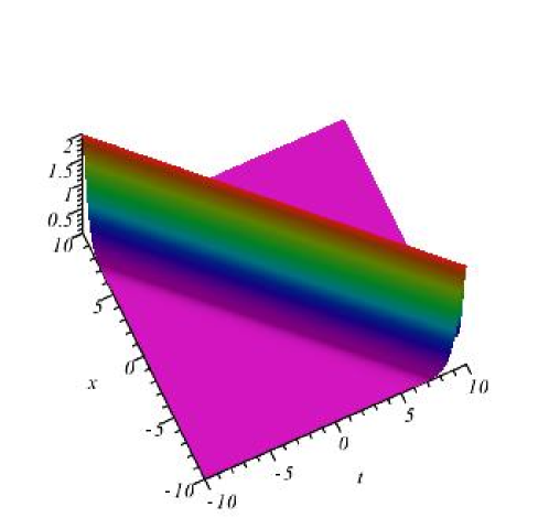
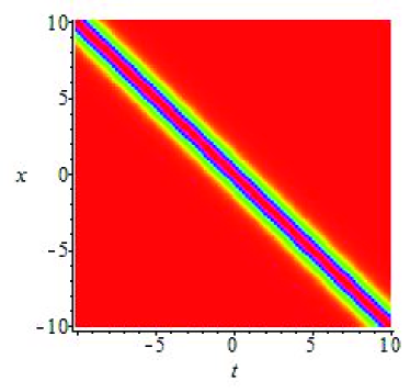
Figure 1: The evolution of a one-soliton solution $q^{[1]}(x,t)$ in the ($x,t$)-plane. Here the parameter is $\lambda_{1}=1$. Panel (b) is a density plot of panel (a).

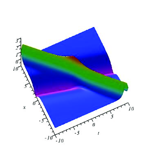
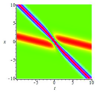
Figure 2: The evolution in the ($x,t$)-plane of a two-soliton solution $q^{[2]}(x,t)$ consisting of one bright soliton and one dark soliton. Here the parameters are $\lambda_{1}=1$ and $\lambda_{3}=\frac{1}{2}$. Panel (b) is a density plot of panel (a).

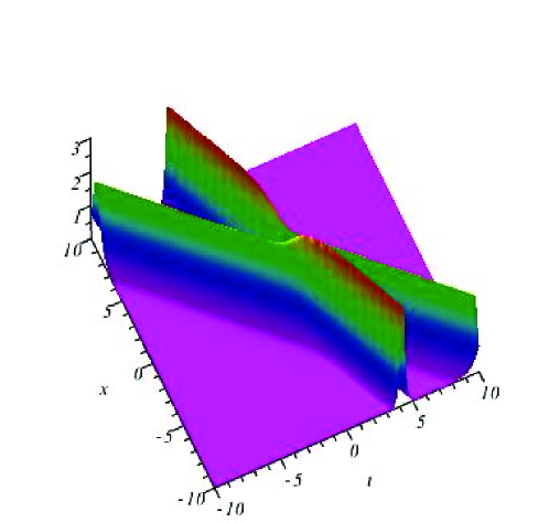
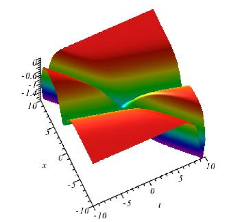
Figure 3: The evolution of other types of two-soliton solutions $q^{[2]}(x,t)$ in the ($x,t$)-plane. Panel (a) shows the evolution of two bright solitons with parameters $\lambda_{1}=\frac{3}{2}$ and $\lambda_{3}=-1$, and panel (b) diplays the evolution of two dark solitons with parameters $\lambda_{1}=-1$ and $\lambda_{3}=\frac{1}{2}$.

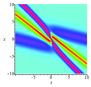
Figure 4: The evolution in the ($x,t$)-plane of a three-soliton solution $q^{[3]}(x,t)$ consisting of two bright solitons and one dark soliton. The parameters are $\lambda_{1}=1$, $\lambda_{3}=\frac{1}{2}$, and $\lambda_{5}=\frac{9}{10}$. Panel (b) is a density plot of panel (a).

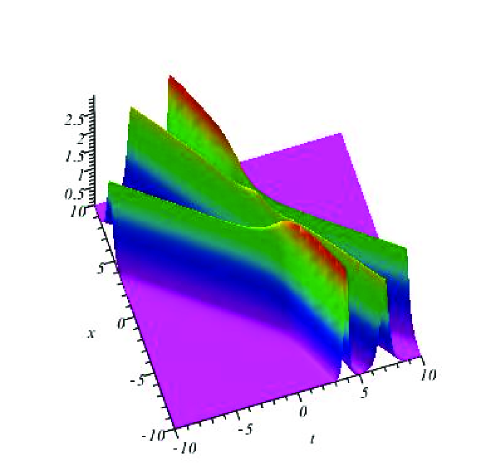
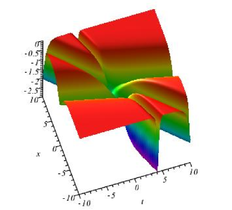
Figure 5: The evolution of other types of three-soliton solutions $q^{[3]}(x,t)$ in the ($x,t$)-plane. Panel (a) shows the evolution of three bright solitons with parameters $\lambda_{1}=\frac{9}{10}$, $\lambda_{3}=-\frac{6}{5}$, and $\lambda_{5}=\frac{3}{2}$, and panel (b) illustrates the evolution of three dark soliotns with parameters $\lambda_{1}=\frac{1}{2}$, $\lambda_{3}=1$, and $\lambda_{5}=-\frac{6}{5}$.

Here $p=2H,\,q=2(\lambda_{3}^{3}t+\lambda_{3}x)$. Three kinds of two-soliton solutions consisting of one bright soliton and one dark soliton, two bright solitons, and two dark solitons are plotted in Fig. 2, Fig. 3(a) and Fig. 3(b), respectively. Similarly, three different cases of three-soliton solutions (see Eq. (16) are also plotted in Figs. 4 and 5, namely two bright solitons and one dark soliton (see Fig. 4), and three bright solitons and three dark solitons (see Fig. 5).

It is easy to see that the denominator in the two-soliton solution is zero in the degenerate case when $\lambda_{1}=\lambda_{3}$. In general, the $n$-soliton solution becomes an indeterminate form $\frac{0}{0}$ when $\lambda_{j}\rightarrow\lambda_{1}\,(j=1,3,5,\cdots,2n-1)$.

However, if we set $\lambda_{j}=\lambda_{1}+\epsilon$ in the $n$-soliton solution, and then we perform the higher-order Taylor expansion (see, for example, Ref. Rj ; Mu ), we then get the $n$-positon solution

$$q_{n-p}=2\frac{N_{2n}^{\prime}}{W_{2n}^{\prime}},$$ (20)

where

$$N_{2n}^{\prime}=(\frac{\partial^{n_{i}-1}}{\partial\epsilon^{n_{i}-1}}|_{\epsilon=0}(N_{2n})_{ij}(\lambda_{1}+\epsilon))_{2n\times 2n},$$

$$W_{2n}^{\prime}=(\frac{\partial^{n_{i}-1}}{\partial\epsilon^{n_{i}-1}}|_{\epsilon=0}(W_{2n})_{ij}(\lambda_{1}+\epsilon))_{2n\times 2n},$$

and $n_{i}=[\frac{i+1}{2}]$,${[i]}$ define the floor function of $i$.

If we set $n=2$, the expression of two-positon solution is given by

$$q_{2-p}=\frac{8\lambda_{1}[(6\lambda_{1}^{3}t+2\lambda_{1}x-1)e^{2H}-(6\lambda_{1}^{3}t+2\lambda_{1}x+1)e^{-2H}]}{-\lambda_{1}^{2}(4x-12\lambda_{1}^{2}t)^{2}-4{\cosh^{2}(2H)}}.$$ (21)

The typical two-positon solution is plotted in Fig. 6. Similarly, we can get the three-positon solution from the three-soliton solution when $n=3$ in Eq. (20) by performing the corresponding Taylor expansion as in the case of the two-positon solution. Because of the complexity of the exact form of the three-positon solution, we do not write down its explicit expression, but we have plotted it in 7.

In what follows we will discuss the unique properties of the positon solutions. According to the expression of the two-positon solution, we see that the denominator of the $q_{2-p}$ cannot be zero, which proves the assertion that the positon solution of the focusing mKdV equation is nonsingular, a result that is completely different from the previous studies about the singular positon solution of the defocusing mKdV equation. At the same time, we can see from Fig. 6(a) the smoothness of the positon solution. The above results inspires us to further study the key features of the positon solution of the focusing mKdV equation. We can easily see that the two-positon solution $q_{2-p}$ is not a travelling wave, and the trajectory of the positon $q_{2-p}$ is not a straight line, that is to say, it is a slowly changing curve. Then, we can explore the dynamics of smooth positons by looking at three main features: the decomposition procedure, the positon trajectories and the corresponding “phase shifts”.

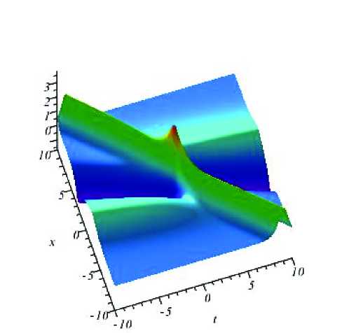
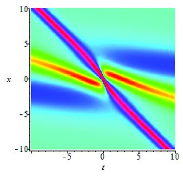
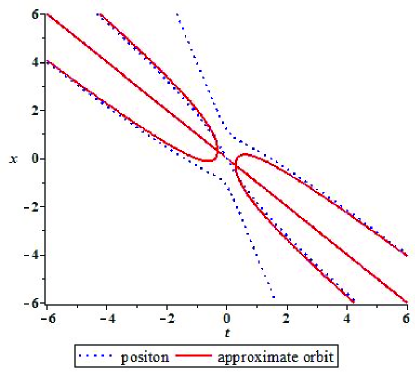
Figure 6: The evolution in the ($x,t$)-plane of a two-positon solution $q_{2-p}(x,t)$ with the parameter $\lambda_{1}=1$. Panel (b) is a density plot of panel (a). Panel (c) shows both the positon trajectories (the two outer blue dotted lines show the location of the positon maxima) and the approximate orbits (red solid lines) of the corresponding single-solitons obtained by the decomposition of the two-positon solution $q_{2-p}(x,t)$. The middle red solid line corresponds to $H=x=t=0$.

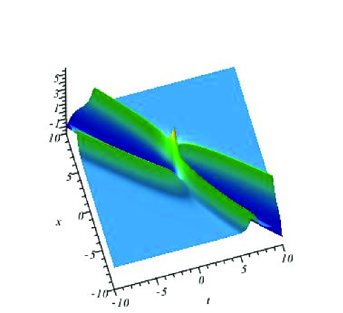
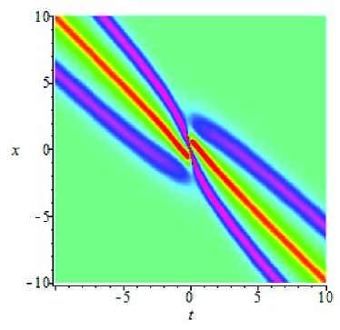
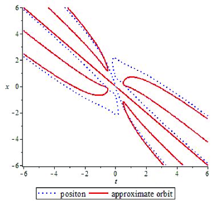
Figure 7: The evolution in the ($x,t$)-plane of a three-positon solution $q_{3-p}(x,t)$ with parameter $\lambda_{1}=1$. Panel (b) is a density plot of panel (a). Panel (c) shows both the positon trajectories (the blue dotted lines) and the approximate orbits (red solid lines) of the corresponding single-solitons obtained by the decomposition of the three-positon solution $q_{3-p}(x,t)$. The middle red solid line corresponds to $H=x=t=0$.

We will set $\lambda_{1}=1$ in order to simplify the calculations. The dynamics of smooth two-positon and three-positon solutions will be analyzed as follows:

• As is well known, a two-soliton solution can be decomposed into a sum of two single solitons with a phase shift at $|t|\gg 0$. The fact stimulates us consider a similar decomposition of the two-positon solution, because a smooth two-positon is obtained in a certain limit of the two-soliton solution solution. Naturally, we introduce the following decomposition of the two-positon solution

  $$q_{2-p}\approx q_{1-s}(H+c_{1})+q_{1-s}(H-c_{1}),\,H=(\lambda_{1}x+\lambda_{1}^{3}t)|_{\lambda_{1}=1}=x+t,$$ (22)

  when $|t|\longrightarrow\infty$

  Here

  $$q_{1-s}(H+c_{1})=\frac{4}{e^{2H+2c_{1}}+e^{-2H-2c_{1}}},$$ (23)

  $$q_{1-s}(H-c_{1})=\frac{4}{e^{2H-2c_{1}}+e^{-2H+2c_{1}}},$$ (24)

  where $q_{1-s}(H)$ is the single-soliton solution given by Eq. (18). The phase shift $c_{1}$ can be determined by substituting (23) and (24) into (22) and considering the corresponding approximation in the neighborhood of $H=0$. It yields

  $$e^{4c_{1}}-2+e^{-4c_{1}}-64t^{2}\approx 0.$$ (25)

  Note that the phase shift is a constant for the two-soliton solution. However, the corresponding “phase shift” $c_{1}$ for the positon solution is an undetermined function of $x$ and $t$. By a simple calculation, $c_{1}=-\frac{\ln(64t^{2})}{4}$ is an approximate solution of Eq. (25) for $|t|>>1$. Therefore a two-positon solution of the focusing mKdV equation can be decomposed as

  $$q_{2-p}\approx q_{1-s}(H+\frac{\ln(64t^{2})}{4})+q_{1-s}(H-\frac{\ln(64t^{2})}{4}),$$ (26)

  when $|t|\longrightarrow\infty$. Here, $H=x+t$, and very good approximate trajectories are two curves defined by $x+t\pm\frac{\ln(64t^{2})}{4}=0$. By comparing with the correponding decomposition of a multi-soliton solution into several single soliton solutions, the appearance of the variable “phase shift” in the decomposition of multi-positon solution into several single-soliton solutions is the key difference between the two decomposition processes.

• For a three-positon solution, we get

  $$q_{3-p}\approx q_{1-s}(H+c_{2})+q_{1-s}(H-c_{2})+q_{1-s}(H),$$ (27)

  when $|t|\longrightarrow\infty$ (here $H=(\lambda_{1}x+\lambda_{1}^{3}t)|_{\lambda_{1}=1}=x+t$ as before). Certainly, the phase shift $c_{2}$ still is an undetermined function of $x$ and $t$. Here we have $c_{2}=\frac{\ln 1024t^{4}}{4}$, and thus very good approximate trajectories are the three curves defined by $x+t\pm\frac{\ln 1024t^{4}}{4}=0$ and $x+t=0$.

4 Summary and discussion

In this paper, a determinant representation of the $n$-fold Darboux transformation $T_{n}$ of the focusing real mKdV equation was given. Using this representation, we have obtained the $n$-soliton solution $q^{[n]}$, and thus we explicitly provided the one-, two-, and three-soliton solutions. Furthermore, a general expression of the smooth, nonsingular multi-positon solution of the focusing mKdV equation was calculated by using a certain Taylor expansion in the corresponding determinant representation of the multi-soliton solution (see Eq. (20)). Finally, we further analyzed the unique properties of the positon solution of the focusing mKdV equation from three points of view: the decomposition procedure, the approximate trajectories, and the corresponding “phase shifts”. By comparing the case of the decomposition of the multi-soliton solution into single solitons with that of the decomposition of the multi-positon solution into single solitons we arrive at the interesting result that in the latter case the “phase shifts” are variable and the approximate trajectories are not straight lines (see Figs. 6 and 7). It is worth mentioning that Figs. 2 to 5 show that we cannot get pure bright or dark solitons when all the eigenvalues of multi-soliton solutions are positive numbers or are negative ones. This facts implies naturally that a multi-positon solution is a combination of several bright and dark solitons, see the two-positons shown in Fig. 6 and the three-positons shown in Fig. 7. This interesting result comes from the fact that the multi-positon solution is obtained in the special limit when the eigenvalues $\lambda_{j}$ ($j=3,5,\cdots$) tend to the same eigenvalue $\lambda_{1}$.

We may conclude that the obtained nonsingular multi-positon solutions of the focusing mKdV equation will undoubtedly be useful for further studies in this area and will give insights in modeling a diverse set of nonlinear wave phenomena in many relevant physical settings.

From our study it is clear that the smooth $n$-positon solution is expressed by a mixture of polynomial and hyperbolic functions, similar to the multi-pole solutions of the real and complex mKdV and the NLS equations, which were reported during the past three decades by using the classical inverse scattering and Hirota methods multi-pole mKdV -focusing . Comparing our results with the known results we would like to point out the following: 1) Equation (20) provides a simple closed formula to calculate the $n$-positon solution; 2) Equations (26) and (27) provide simple and direct expressions for the decomposition of multi-positon solutions into single solitons, and also show more precise formulas for the “phase shifts” and soliton trajectories. The corresponding soliton trajectories have been illustrated numerically in Figs. 6 and 7. Moreover, it is worthy to further study the relationship between the smooth positon solutions and the multi-pole solutions for other physically relevant nonlinear evolution equations.

- (1) Russell, J.S.: Report on Waves; Rept. Fourteenth Meeting of the British Association for the Advancement of Science. J. Murray, London, pp. 311–390 (1844)
- (2) Korteweg, D.J., de Vries, G.: On the change of form of long waves advancing in a rectangular canal, and on a new type of long stationary waves. Phil. Mag. 39, 422–443 (1895)
- (3) Gardner, C.S., Morikawa, G.K.: Similarity in the asymptotic behaviour of collision-free hydromagnetic waves and water waves. Courant Ins. Math. Sci., Res. Report NYO-9082 (1960)
- (4) Washimi, H., Taniuti, T.: Propagation of ion-acoustic solitary waves of small amplitude. Phys. Rev. Lett. 17, 996–998 (1996)
- (5) Kruskal, M.D.: Asymptotology in numerical computation: progress and plans on the Fermi-Pasta-Ulam problem. Phys. IBM Data Processing Division, White Plains, N. Y., 43–62 (1965)
- (6) Zabusky, N.J.: A synergetic approach to problems of nonlinear dispersive wave propagation and interaction, in Nonlinear partial differential equations: A symposium on methods of solution, Ed. by W. F. Ames, pp. 223-258, Academic Press, New York-London, 1967
- (7) Sjöberg, A.: On the Korteweg-de Vries equations: Existence and uniqueness. J. Math. Anal. Appl. 29, 569–579 (1970)
- (8) Miura, R.M.: Korteweg-de Vries equation and generalizations. I. A remarkable explicit nonlinear transformation. J. Math. Phys. 9, 1202–1204 (1968)
- (9) Miura, R.M.: The Korteweg-de Vries equation: a survey of results. SIAM Rev. 18, 412–459 (1976)
- (10) Kivshar, Y.S., Malomed, B.A.: Solitons in a system of coupled Korteweg-de Vries equations. Wave Motion 11, 261–269 (1989)
- (11) Grimshaw R., Malomed, B.A.: A new type of gap soliton in a coupled KdV-wave system. Phys. Rev. Lett. 72, 949–953 (1994)
- (12) Grimshaw, R., Malomed, B.A., Tian, Xin: Gap-soliton hunt in a coupled Korteweg-de Vries system. Phys. Lett. A 201, 285–292 (1995)
- (13) Gottwald, G., Grimshaw, R., Malomed, B.: Parametric envelope solitons in coupled Korteweg-de Vries equations. Phys. Lett. A 227, 47–54 (1997)
- (14) Espinosa-Ceron, A., Malomed, B.A., Fujioka, J., Rodriguez, R.F.: Symmetry breaking in linearly coupled KdV systems. Chaos 22, 033145 (2012)
- (15) Leblond, H., Mihalache, D.: Few-optical-cycle solitons: Modified Korteweg-de Vries sine-Gordon equation versus other non-slowly-varying-envelope-approximation models. Phys. Rev. A 79, 063835 (2009)
- (16) Leblond, H., Mihalache, D.: Few-optical-cycle dissipative solitons. J. Phys. A 43, 375205 (2010)
- (17) Triki, H., Leblond, H., Mihalache, D.: Derivation of a modified Korteweg-de Vries model for few-optical-cycles soliton propagation from a general Hamiltonian. Opt. Commun. 285, 3179–3186 (2012)
- (18) Leblond, H., Triki, H., Mihalache, D.: Theoretical studies of ultrashort-soliton propagation in nonlinear optical media from a general quantum model. Rom. Rep. Phys. 65, 925–942 (2013)
- (19) Leblond H., Mihalache, D.: Models of few optical cycle solitons beyond the slowly varying envelope approximation. Phys. Rep. 523, 61–126 (2013)
- (20) Frantzeskakis, D.J., Leblond, H., Mihalache, D.: Nonlinear optics of intense few-cycle pulses: An overview of recent theoretical and experimental developments. Rom. J. Phys. 59, 767–784 (2014)
- (21) Mihalache, D.: Localized structures in nonlinear optical media: A selection of recent studies. Rom. Rep. Phys. 67, 1383–1400 (2015)
- (22) Terniche, S., Leblond, H., Mihalache, D., Kellou, A.: Few-cycle optical solitons in linearly coupled waveguides. Phys. Rev. A 94, 063836 (2016)
- (23) Leblond, H., Grelu, P., Mihalache, D.: Models for supercontinuum generation beyond the slowly-varying-envelope approximation. Phys. Rev. A 90, 053816 (2014)
- (24) Leblond, H., Grelu, P., Mihalache, D., Triki, H.: Few-cycle solitons in supercontinuum generation. Eur. Phys. J. Special Topics 225, 2435–2451 (2016)
- (25) Lonngren, K.E.: Ion acoustic soliton experiments in a plasma. Optical and Quantum Electronics. 30, 615–630 (1998)
- (26) Watanbe, S.: Ion acoustic soliton in plasma with negative ion. J. Phys. Soc. Jpn. 53, 950–956 (1984)
- (27) Helal, M.A.: Soliton solution of some nonlinear partial differential equations and its applications in fluid mechanics. Chaos Solitons & Fractals 13, 1917–1929 (2002)
- (28) Ono, H.: Soliton fission in anharmonic lattices with reflectionless inhomogeneity. J. Phys. Soc. Jpn. 61, 4336–4343 (1992)
- (29) Khater, A.H., El-Kalaawy, O.H., Callebaut, D.K.: Bäcklund transformations and exact solutions for Alfven solitons in a relativistic electron-positron plasma. Phys. Scr. 58, 545–548 (1998)
- (30) El-Shamy, E.F.: Dust-ion-acoustic solitary waves in a hot magnetized dusty plasma with charge fluctuations. Chaos Solitons & Fractals. 25, 665–674 (2005)
- (31) Ralph, E.A.; Pratt, L.: Predicting eddy detachment for an equivalent barotropic thin jet. J. Nonlinear Sci. 4, 355–374 (1994)
- (32) Komatsu, T.S., Sasa, Shin-ichi: Kink soliton characterizing traffic congestion. Phys. Rev. E 52, 5574–5582 (1995)
- (33) Ge, H.X., Dai, S.Q., Xue, Y., Dong, L.Y.: Stabilization analysis and modified Korteweg-de Vries equation in a cooperative driving system. Phys. Rev. E 71, 066119 (2005)
- (34) Ziegler, V., Dinkel, J., Setzer, C., Lonngren, K.E.: On the propagation of nonlinear solitary waves in a distributed Schottky barrier diode transmission line. Chaos Solitons & Fractals. 12, 1719–1728 (2001)
- (35) Wazwaz, A.M., Xu, G.Q,: An extended modified KdV equation and its Painlevé integrability. Nonl. Dyn. 86, 1455–1460 (2016)
- (36) Wazwaz, A.M., El-Tantawy, S.A.: A new integrable (3+1)-dimensional KdV-like model with its multiple-soliton solutions. Nonl. Dyn. 83, 1529–1534 (2016)
- (37) Mirzazadeh, M., Eslami, M., Biswas, A.: 1-Soliton solution of KdV6 equation. Nonl. Dyn. 80, 387–396 (2015)
- (38) Mirzazadeh, M., Arnous, A.H., Mahmood, M.F., Zerrad, E., Biswas, A.: Soliton solutions to resonant nonlinear Schrödinger’s equation with time-dependent coefficients by trial solution approach. Nonl. Dyn. 81, 277–282 (2015)
- (39) Yuan, F., Rao, J.G., Porsezian, K., Mihalache, D., He, J.S.: Various exact rational solutions of the two-dimensional Maccari’s system. Rom. J. Phys. 61, 378–399 (2016)
- (40) Triki, H., Leblond, H., Mihalache, D.: Soliton solutions of nonlinear diffusion-reaction-type equations with time-dependent coefficients accounting for long-range diffusion. Nonl. Dyn. 86, 2115–2126 (2016)
- (41) Liu, Y.B., Fokas, A.S., Mihalache, D., He, J.H.: Parallel line rogue waves of the third-type Davey-Stewartson equation. Rom. Rep. Phys. 68, 1425–1446 (2016)
- (42) Porubov, A.V., Fradkov, A.L., Bondarenkov, R.S., Andrievsky, B.R.: Localization of the sine-Gordon equation solutions. Commun. Nonl. Sci. Numer. Simul. 39, 29–37 (2016).
- (43) Chen, S.H., Grelu, P., Mihalache, D., Baronio, F.: Families of rational soliton solutions of the Kadomtsev-Petviashvili equation. Rom. Rep. Phys. 68, 1407–1424 (2016)
- (44) He, J.S., Zhang, H.R., Wang, L.H., Porsezian, K., Fokas, A.S.: Generating mechanism for higher-order rogue waves. Phys. Rev. E 87, 052914 (2013)
- (45) Mu, G., Qin, Z., Grimshaw, R.: Dynamics of rogue waves on a multisoliton background in a vector nonlinear Schrödinger equation, SIAM J. Appl. Math. 75, 1–20 (2015)
- (46) Chowdury, A., Ankiewicz, A., Akhmediev, N.: Periodic and rational solutions of modified Korteweg-de Vries equation. Eur. Phys. J. D 70, 104 (2016)
- (47) Weiss, J., Tabor, M., Carnvale, G.: The Painlevé property for partial differential equation. J. Math. Phys. 24, 522–526 (1983)
- (48) Yao, R.X., Qu, C.Z., Li, Z.B.: Painlevé property and conservation laws of multi-component mKdV equations. Chaos Solitons & Fractals. 22, 723–730 (2004)
- (49) Li, D.S., Yu, Z.S., Zhang, H.Q.: New soliton-like solutions to variable coefficients mKdV equation. Commmun. Theor. Phys. 42, 649–654 (2004)
- (50) Yeung, T.C.A., Fung, P.C.W.: Hamiltonian formulation of the inverse scattering method of the modified KdV equation under the non-vanishing boundary condition u(x, t) to b as x to + or - infinity. J. Phys. A 21, 3575–3592 (1988)
- (51) He, J.S., Wang, L.H., Li, L.J., Porsezian, K., Erdélyi, R.: Few-cycle optical rogue waves: Complex modified Korteweg-de Vries equation. Phys. Rev. E 89, 062917 (2014)
- (52) Matveev, V.B.: Generalized Wronskian formula for solutions of the KdV equations: first applications. Phys. Lett. A 166, 205–208 (1992)
- (53) Matveev, V.B.: Positon-positon and soliton-positon collisions: KdV case. Phys. Lett. A 166, 209–212 (1992)
- (54) Chow, K.W., Lai, W.C., Shek, C.K., Tso, K.: Positon-like solutions of nonlinear evolution equations in (2+1) dimensions. Chaos Solitons & Fractals. 9, 1901–1912 (1998)
- (55) Dubard, P., Gaillard, P., Klein, C., Matveev, V.B.: On multi-rogue wave solutions of the NLS equation and positon solutions of the KdV equation. Eur. Phys. J. Special Topics 185, 247–258 (2010)
- (56) Stahlofen, A.A.: Positons of the modified Korteweg-de Vries equation. Annalen der Physik 504, 554–569 (1992)
- (57) Maisch, H., Stahlofen, A.A.: Dynamic properties of positons. Phys. Scripta. 52, 228–236 (1995)
- (58) Beutler, R.: Positon solutions of the sine-Gordon equation. J. Math. Phys. 34, 3081–3109 (1993)
- (59) Stahlofen, A.A., Matveev, V.B.: Positons for the Toda lattice and related spectral problems. J. Phys. A: Math. Gen. 28, 1957–1965 (1995)
- (60) Wadati, M.: The exact solution of the modified Korteweg-de Vries equation. J. Phys. Soc. Jpn. 32, 1681–1687 (1972)
- (61) Wadati, M.: The modified Korteweg-de Vries equation. J. Phys. Soc. Jpn. 34, 1289–1296 (1973)
- (62) Masataka, W., Hirota, R.: Soliton solutions of a coupled modified KdV equations. J. Phys. Soc. Jpn. 66, 577–588 (1997)
- (63) Ablowitz, M.J., Kaup, D.J., Newell, A.C., Segur, H.: The inverse scattering transform-Fourier analysis for nonlinear problems. Stud. Appl. Math. 53, 249–315 (1974)
- (64) Drinfel’d, V.G., Sokolov, V.V.: Lie algebras and equations of Korteweg-de Vries type, Itogi Nauki i Tekhniki, Akad. Nauk SSSR, Vsesoyuz. Inst. Nauchn. i Tekhn. Inform., Moscow (in Russian), Current Problems in Mathematics 24, 81–180 (1984)
- (65) Terng, C.L., Uhlenbeck, K.: Bäcklund transformations and loop group actions, Comm. Pure Appl. Math.53 , 1–75 (2000)
- (66) Terng, C.L., Uhlenbeck, K.: The KdV flows, J. Fixed Point Theory and its Applications 10, 37–61 (2011).
- (67) Wadati, M., Ohkuma, K.: Multiple-pole solutions of the modified Korteweg-de Vries equation. J. Phys. Soc. Jpn. 51, 2029–2035 (1982)
- (68) Olmedilla, E.: Multiple-pole solutions of the nonlinear Schrödinger’s equation. Physica D 25, 330–346 (1987)
- (69) Takahashi, H., Konno, K.: Initial value problems of double pole and breather solutions for the modified Korteweg-de Vries equation. J. Phys. Soc. Jpn. 58, 3585–3588 (1989)
- (70) Takahashi, M., Konno, K.: N-double pole solution for the modified Korteweg-de Vries equation by the Hirota’s method. J. Phys. Soc. Jpn. 58, 3505–3508 (1989)
- (71) Karlsson, M., Kaup, D.J., Malomed B.A.: Interactions between polarized soliton pulses in optical fibers: exact solutions. Phys. Rev. E 54, 5802–5808 (1996)
- (72) Shek, C.M., Grimshaw, R.H.J., Ding, E., Chow, K.W.: Interactions of breathers and solitons of the extended Korteweg-de Vries equation. Wave Motion 43, 158–166 (2005)
- (73) Alejo, M.A., Focusing mKdV breather solutions with nonvanishing boundary condition by the inverse scattering method. J. Nonl. Math. Phys. 19, 125009 (2012)