Interferometric Monitoring of Gamma-ray Bright AGNs: S5 0716+714

Abstract

We present the results of very long baseline interferometry (VLBI) observations of gamma-ray bright blazar S5 0716+714 using the Korean VLBI Network (KVN) at the 22, 43, 86, and 129 GHz bands, as part of the Interferometric Monitoring of Gamma-ray Bright AGNs (iMOGABA) KVN key science program. Observations were conducted in 29 sessions from January 16, 2013 to March 1, 2016, with the source being detected and imaged at all available frequencies. In all epochs, the source was compact on the milliarcsecond (mas) scale, yielding a compact VLBI core dominating the synchrotron emission on these scales. Based on the multi-wavelength data between 15 GHz (Owens Valley Radio Observatory) and 230 GHz (Submillimeter Array), we found that the source shows multiple prominent enhancements of the flux density at the centimeter (cm) and millimeter (mm) wavelengths, with mm enhancements leading cm enhancements by -16$\pm$8 days. The turnover frequency was found to vary between 21 to 69 GHz during our observations. By assuming a synchrotron self-absorption model for the relativistic jet emission in S5 0716+714, we found the magnetic field strength in the mas emission region to be $\leq 5$ mG during the observing period, yielding a weighted mean of $1.0\pm 0.6$ mG for higher turnover frequencies (e.g., $>$45 GHz).

1 Introduction

A radio-loud active galactic nucleus (AGN) is a very compact region in a galaxy with a super-massive black hole (SMBH, $M_{\rm BH}\approx 10^{6}-10^{9}M_{\odot}$) in its central part, emitting at extremely high luminosity with a relativistic jet (Radio-quiet AGNs also sometimes have a jet) (see e.g., Krolik, 1999). Blazars are a subclass of AGN with a relativistic jet directed toward the observer (i.e., small viewing angle). Some of the major physical properties of blazars across the entire electromagnetic spectra from radio to gamma-rays include flux density variability on time scales of hours to years (see e.g., Boettcher et al., 2012, for review).

The observed variability suggests a possible connection to different regions of the jet e.g., rapid variations being connected to the innermost regions of relativistic jets, and slow variations being related to downstream jet emission (on parsec scales). High-resolution multi-frequency very long baseline interferometry (VLBI) observations enable us to investigate synchrotron radiation. Radio emission is thought to be due to synchrotron emission from a relativistic jet on the milliarcsecond (mas) scale, yielding a plethora of observables such as flux density, source structure, and polarization properties, which can help us to study the physical conditions in the jet in the vicinity of the SMBH.

S5 0716+714 is one of the most active blazars known, with a flat spectrum, located at z $\sim$ 0.127 (Stadnik & Romani, 2014). The remarkable properties of this source are its extreme flux density variability, such as broadband flaring on a time scale of months (Raiteri et al., 2003; Nesci et al., 2005; Rani et al., 2013) and its intraday variability (IDV), possibly from an extrinsic origin for the cm-wavelength IDV (Wagner et al., 1996; Liu et al., 2012) and from an intrinsic origin for mm-wavelength IDV (Kraus et al., 2003; Lee et al., 2016a). Bhatta et al. (2015) detected five-hour-long microflares in flux density and polarization in optical band with the Whole Earth Blazar Telescope (WEBT) during the iMOGABA observing campaign. This was interpreted by propagation and compression of a small-scale but strong shock within the jet. Martí-Vidal et al. (2016) computed core-shift between 14.4 GHz and 43 GHz by VLBI observations for S5 0716+714. They found that the core shift is roughly aligned with the jet direction because the core shift shall be aligned with the highest magnetic field and/or particle density gradient, which are given in the direction longitudinal to the jet.

In general, flares lasting approximately months are explained by the shock-in-jet model (Marscher & Gear, 1985). VLBI studies of the source on the mas scales show a core-dominated jet (Bach et al., 2005; Rastorgueva et al., 2011) and suggest a connection between the jet kinematics and the observed broadband flares (Rani et al., 2015). Based on mm-VLBI observations and gamma-ray monitoring with Fermi/LAT (Large Area Telescope) of S5 0716+714, it was reported that variation of the gamma-ray flux is correlated with position angle variations in the VLBI jet. Additionally, they found variation in the mm-VLBI core flux density, indicating that the high-energy emission originates upstream of the mm-VLBI core (Rani et al., 2014). In a broadband long-term flare study of S5 0716+714, Rani et al. (2013) found that flares in the jet propagate from the high-energy emission region to the low-energy emission regions with a time delay of $\sim$65 days due to opacity, yielding the evolution of the spectra following the shock-in-jet model, the emission region size of a few $\mu$as, and a magnetic field of a few mG. However, these multi-frequency studies may have possible uncertainty in the derived spectral information for S5 0716+714, as the multi-frequency observations were conducted only quasi-simultaneously.

In this paper, we report the results of simultaneous multi-frequency VLBI monthly monitoring observations of S5 0716+714 over three years using the Korean VLBI Network (KVN) at 22, 43, 86, and 129 GHz. These observations enable us to investigate the spectral information of the synchrotron emission regions on the mas scale. In Section 2, we describe the VLBI observations with KVN and the data reduction procedures used, and in Section 2.5, we summarize the multi-wavelength data collected for our study. We present the results of the observations and analysis in Section 3, followed by the discussion in Section 4. Finally, a summary of the paper is presented in Section 5.

2 Observations and Data Reduction

2.1 Observations

VLBI observations of S5 0716+714 were performed as part of the Interferometric MOnitoring of Gamma-ray Bright AGNs (iMOGABA) project (Lee et al., 2013, 2016b). More than 30 radio-loud AGNs are monitored monthly and simultaneously at 22, 43, 86, and 129 GHz, with the first observation occurring on December 5, 2012 (MJD 56266), using the Korean VLBI Network (KVN) (Lee et al., 2011, 2014). The KVN is a 500-km VLBI array consisting of three identical 21-m radio telescopes: the KVN Yonsei (KY), the KVN Ulsan (KU), and the KVN Tamna (KT). The typical spatial resolutions are 6, 3, 1.5, and 1 milliarcsecond (mas) at 22, 43, 86, and 129 GHz, respectively.

The iMOGABA observations used for this paper were conducted during a period of more than three years from January 16, 2013 (MJD 56308) to March 1, 2016 (MJD 57448) with a mean cadence of $\sim$30 days. All sources were observed in every 24-hour session with 1-8 five-min scans. The observing frequencies are 21.700–21.764 GHz, 43.400–43.464 GHz, 86.800–86.864 GHz, and 129.300–129.364 GHz, in left circular polarization (LCP), yielding a total bandwidth of 256 MHz and a bandwidth of 64 MHz for each band (when observed at four frequency bands). The starting frequencies of each band have integer-ratios for the application of the frequency phase transfer (FPT) technique for faint sources. The FPT technique was successfully demonstrated for iMOGABA observations by Algaba et al. (2015). To trace the opacity of the atmosphere during each 24-hr observation, hourly sky tipping curve measurements were performed at each antenna every hour by measuring the system temperatures at the following eight elevations: 18.21^∘, 20.17^∘, 22.62^∘, 25.77^∘, 30.00^∘, 36.03^∘, 45.58^∘, and 65.38^∘. Antenna pointing offsets were corrected for every scan through cross-scan observations of target sources. During each scan, the received signals were digitized (i.e., 2-bit quantized) by digital samplers, requantized, divided into 16 sub-bands (IFs) with a bandwidth of 16 MHz by a digital filter bank, and then recorded by the Mark 5B system at a rate of 1024 Mbps. The recorded data were correlated using the DiFX software correlator in the Korea-Japan Correlator Center (Deller et al., 2007; Lee et al., 2015a).

2.2 Data analysis

The output from the DiFX correlator is the spectrum of the cross-correlation function with a resolution of 0.125 MHz and an accumulation period of 1 s. A post-correlation process was conducted using the National Radio Astronomy Observatory (NRAO) Astronomical Image Processing System (AIPS). Post-correlation processing was done both manually and automatically using the KVN Pipeline. Data were reduced using standard AIPS tasks and with ParselTongue (Kettenis et al., 2006) with the operation of the KVN Pipeline being described in detail by Hodgson et al. (2016). Sensitivity at high frequencies was improved by transferring phase solutions from longer to shorter wavelengths (i.e., FPT) as described by Rioja & Dodson (2011), Rioja et al. (2014), and Algaba et al. (2015).

An antenna-based fringe fit was conducted using the AIPS task FRING. The 5-min scans were split into solution intervals of 30 s. Baseline-based fringe solutions (phase delays and delay rates) were solved for individual IFs at all frequency bands. The baseline-based fringe solutions were used to determine the antenna-based fringe solutions.

Amplitude calibration was performed using the system temperatures measured during the observations. The measured system temperatures were corrected for atmospheric opacity as determined by sky tipping curve measurements conducted every hour during the observations at each telescope. Re-normalization of the fringe amplitudes was done to correct for amplitude distortion due to quantization, and the quantization and re-quantization losses were corrected (Lee et al., 2015a, b). After the amplitude calibration and the re-quantization loss correction, we expect that the uncertainty of the amplitude calibration is within 5 % at 22 and 43 GHz bands (Petrov et al., 2012; Lee et al., 2014, 2015b) and 10-30 % at 86 and 129 GHz bands (Lee et al. in prep.).

2.3 Imaging and model-fitting

Although there are limitations in imaging using visibility data obtained with only three antennas, i.e., only one closure phase for each scan and no closure amplitude, the hybrid mapping for the KVN observations is feasible for discussing the total flux spectral index of such a compact radio source. CLEAN images were produced using the Caltech DIFMAP software. The calibrated uv-data were averaged in terms of the frequency by chopping the band edges (10% of the bandwidth), where severe flux loss arises due to the bandpass shape. The data were then re-averaged in time over 30 seconds at 22, 43, and 86 GHz and over 10 seconds at 129 GHz, taking into account the coherence time at each frequency band, and expecting decoherence loss of up to 30 % at 86-129 GHz bands (Lee et al. in prep.). Outliers in the amplitude of the averaged uv-data were flagged out. For some epochs, the uv-data contained considerable antenna pointing offsets due to anomalous refraction, which caused significant antenna-based flux loss. A single circular Gaussian model was used to fit and phase-self-calibrate the averaged uv-data. The self-calibrated data were again fitted with a set of CLEAN point source models and self-calibrated with respect to the CLEAN models. The iteration of CLEAN and self-calibration were run until the residual noise in the CLEAN image is comparable to the Gaussian random noise.

The residual noise was investigated to evaluate the image quality, as described in Lee et al. (2016b). Under the assumption that the residual noise of the ideal CLEAN image is random noise and hence should have a Gaussian distribution, the noise in the final CLEAN image could be evaluated using an image quality factor, i.e., the ratio of the image noise RMS to its mathematical expectation, $\xi_{\rm r}=s_{\rm r}/s_{\rm{r,exp}}$, where $|s_{\rm r}|$ is the maximum absolute flux density in the residual image and $|s_{\rm r,exp}|$ is the expectation of $s_{\rm r}$. For residual random Gaussian noise with a zero mean, the expectation of $s_{\rm r}$ is $|s_{\rm{r,exp}}|=\sigma_{\rm r}{\left[\sqrt{2}\ln{\left(\frac{N_{\rm pix}}{\sqrt{2\pi}\sigma_{\rm r}}\right)}\right]}^{1/2}$, where $N_{\rm pix}$ is the total number of pixels in the image and $\sigma_{\rm r}$ denotes the image noise rms. When the residual noise is close to Gaussian noise, the image quality factor $\xi_{\rm r}\rightarrow 1$; when the residual image still contains a source structure, $\xi_{\rm r}>1$; and when the final image has a large number of degrees of freedom, $\xi_{\rm r}<1$ (Lobanov et al., 2006). We found that the values of $\xi_{\rm r}$ of the final CLEAN images obtained in this paper are in the range of 0.54-0.74 at 22 GHz, 0.49-0.79 at 43 GHz, 0.41-0.70 at 86 GHz, and 0.45-0.71 at 129 GHz, as shown in Figure 1 and as summarized in Table 1, implying that the images adequately represent the structure observed.

Given that the target source S5 0716+714 is a circumpolar source, the uv-distribution fill only a limited range, i.e., the lack of relative short baseline giving rise to a lack of data for the innermost region in the uv-plane. This may cause a missing-flux problem in the CLEANed total flux density: a larger-scale structure of the source may be resolved out and hence the flux density for the larger-scale structure may miss. However, for such a compact radio source on mas-scales to arcsecond-scales, the missing-flux effect may not be significant. We expect that for future studies, single-dish (zero spacing) observations should be accompanied for properly measuring the total flux density of the source free from the missing-flux effect.

The visibility data of the final CLEAN images were used for fitting with circular Gaussian models. From the Gaussian model-fitting step, a set of fit parameters were obtained, as follows: $S_{\rm tot}$ (total flux density), $S_{\rm peak}$ (peak flux density ), $\sigma_{\rm rms}$ (post-fit rms), $d$ (size), $r$ (radial distance, for jet components), and $\theta$ (position angle, measured for jet components, with respect to the location of the core component), as summarized in Table 2.

The uncertainties in Table 2 were obtained while taking into account the signal-to-noise ratio during the detection of each component, and following Lee et al. (2016b). The minimum resolvable size was estimated for each component according to Lobanov (2005). The minimum resolvable size was used to determine then upper limit of the component size when the fitted component size $d$ was smaller than the minimum resolvable size. The upper limit of the size was also used to estimate the lower limit of the brightness temperature $T_{\rm b}$, as established by $T_{\rm b}=\frac{2\ln{2}}{{\pi}{k}}\frac{S_{\rm tot}\lambda^{2}}{d^{2}}(1+z)$, where $\lambda$ is the wavelength of the observation, $z$ is the redshift, and $k$ is the Boltzmann constant.

2.4 Images and model-fit parameters

We detected S5 0716+714 during 29 observing sessions for an observing period of more than three years, from January 16, 2013 to March 1, 2016, in at least one frequency band, yielding 89 VLBI images. These were 29 images at 22 GHz, 25 images at 43 GHz, 23 images at 86 GHz, and 11 images at 129 GHz. These are the first simultaneous multi-frequency VLBI long term monitoring images, yielding a very compact core-dominated structure on the mas scale.

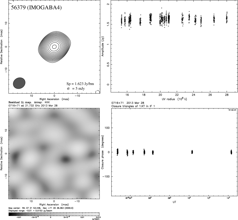
Figure 2: Example of contour map (upper left), residual map (lower left), the visibility amplitude against uv-radius (upper right), and the closure phase as function of time (lower right), at 22 GHz band obtained in March 28, 2013 (MJD 56379). The axes of the contour and residual maps show the relative offset from the center of image in milliarcsecond. Minimum contour level is shown in the lower-right corner of the contour map. The contours have a logarithmic spacing and are drawn at -1, 1, 1.4,…,$1.4^{n}$ of the minimum contour level. In the upper right panel, the X-axis shows the uv-distance in $10^{6}\lambda$, the Y-axis represents the visibility amplitude (correlated flux density) in Jy. In the lower right panel, the X-axis shows the time in UT hour, and the Y-axis represents the closure phase in degree. Image parameters of each image are summarized in Table 1.

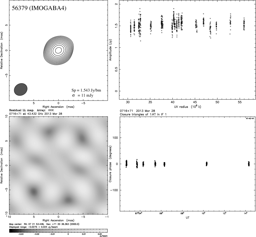
Figure 2: Example of contour map (upper left), residual map (lower left), the visibility amplitude against uv-radius (upper right), and the closure phase as function of time (lower right), at 43 GHz band obtained in March 28, 2013 (MJD 56379) (continued)

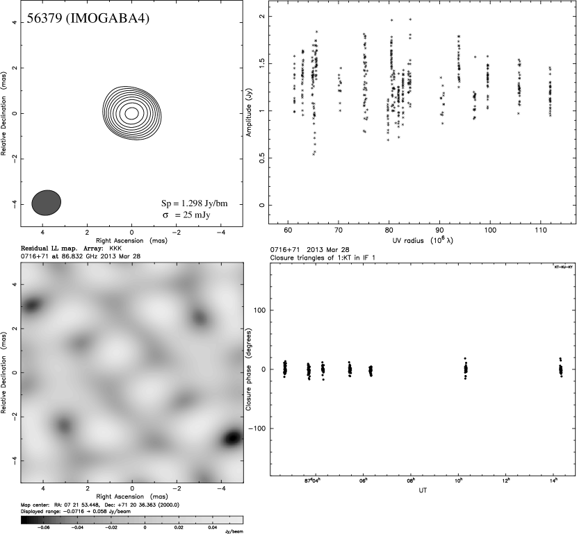
Figure 2: Example of contour map (upper left), residual map (lower left), the visibility amplitude against uv-radius (upper right), and the closure phase as function of time (lower right), at 86 GHz band obtained in March 28, 2013 (MJD 56379) (continued)

Figure 2 shows the representative CLEAN contour maps of S5 0716+714 for the 22, 43, 86, and 129 GHz bands. For each VLBI image, a set of four plots is presented: a contour map (top left panel), a residual map (bottom left panel), a plot of the visibility amplitude against the uv-radius (top right panel), and a plot of closure phase (bottom right panel). The contour map is drawn with a relative coordinate in units of milliarcseconds (mas). The contour map is centered on the brightest emission region (VLBI core). General information about each image is provided in the map, including the FWHM of the restoring beam (the shaded ellipse) in the lower left corner, and the peak flux density together with the RMS noise level in the lower right corner of the map. The contours are drawn with logarithmic spacing, starting with three times the RMS noise level, and increasing as -1, 1, 1.4,…,$1.4^{n}$ of the lowest contour level. The plot of the visibility amplitude (top right of each set) is in units of Jy for the visibility amplitude (i.e., correlated flux density) and of $10^{6}\lambda$, where $\lambda$ is the observing wavelength, for the uv-radius (i.e., the length of the baseline used to obtain the corresponding visibility point).

Table 1 lists the fitted parameters of the contour maps presented in Figure 2, including the observing frequency band, the parameters of the restoring beam (the size of the major axis $B_{\rm maj}$, the minor axis $B_{\rm min}$ and the position angle of the beam $B_{\rm PA}$), the total flux $S_{\rm KVN}$, the peak flux density $S_{\rm p}$, the off-source RMS $\sigma$, the dynamic range of image $D$, and the quality $\xi_{\rm r}$ of the residual noise in the image.

Table 2 lists the parameters of each model-fit component and the measured brightness temperature $T_{\rm b}$. The uncertainties of each modelfit parameter are estimated as described in Section 2.3. The upper limits of size $d$, and the lower limits of brightness temperature $T_{\rm b}$ are in italic font with flag symbols.

2.5 Multi-wavelength data

We collected the multi-wavelength flux density data at 15 GHz, 43 GHz, and 230 GHz of S5 0716+714 obtained as the Owens Valley Radio Observatory (OVRO), the Very Long Baseline Array (VLBA), and the Submillimeter Array (SMA), respectively, from January 2013 to March 2016, as follows.

2.5.1 OVRO 15 GHz data

The 1500 blazar monitoring program at 15 GHz with the 40-m radio telescope at the OVRO began in late 2007, approximately one year before the start of the Large Area Telescope (LAT) science operation (Richards et al., 2011). This monitoring is large-scale and fast-cadence monitoring conducted approximately twice a week with a minimum flux density of 4 Jy and with 3% typical uncertainty. S5 0716+714 is one of the published observing sources starting in early 2008.

2.5.2 VLBA 43 GHz data

The VLBA Boston University Blazar monitoring program observes a total of 36 AGNs including 33 blazars and three radio galaxies at 43 GHz mostly once per month (Marscher et al., 2008). This program is conducted to study the kinematics of the innermost parsec-scale jet behavior and to determine the location of gamma-ray emission in the gamma-ray bright AGNs. The peak intensity, the polarized intensity, the CLEAN model files, and the calibrated visibility data files for all observing sources are available publicly on the VLBA-BU-BLAZAR program website. We obtained the total flux densities of S5 0716+714 from the CLEAN model and the calibrated visibility data for comparison with those of the iMOGABA project at 43 GHz.

2.5.3 SMA 230 GHz data

The 230 GHz flux density data were obtained at the Submillimeter Array (SMA), an eight-element interferometer located near the summit of Mauna Kea (Hawaii). S5 0716+714 is included in an ongoing monitoring program at the SMA to determine the flux densities of compact extragalactic radio sources that can be used as calibrators at mm and sub-mm wavelengths (Gurwell et al., 2007). The measured source signal strengths were calibrated against known standards, typically solar system objects (Titan, Uranus, Neptune, or Callisto). Data from this program are updated regularly and are available on the SMA website.

3 Results and analysis

3.1 Multi-wavelength light curves

Figure 3 shows multi-wavelength light curves of S5 0716+714 obtained during 2013.04 - 2016.16 using the OVRO 40-m radio telescope at 15 GHz, the KVN at 22-129 GHz, the VLBA at 43 GHz, and the SMA at 230 GHz.

3.1.1 The 15 GHz light curve

The 15 GHz light curve is well sampled with a mean cadence of 7 days, which appears to start on a peak or in a middle of a decaying phase of a major flare on 2012.97 with a flux density of $\sim$3.6 Jy and then reaches its minimum level 126 days later on 2013.32. The light curve shows a prominent second flare with a peak flux density of $\sim$3.6 Jy again on 2013.54, before rapidly decaying to a flux density of $\sim$2 Jy between 2013.54-2013.73. This was followed by a more moderate decrease to a flux density of $\sim$1.3 Jy on 2014.22. After these two major flares and the mild decline, the 15 GHz light curve shows relatively small but more rapid flux enhancements than the major flares between 2014.39 and 2015.34, reaching a flux density of $\sim$1.3 Jy. Another flare, broader in time and not as prominent in flux density, is also seen after 2015.62. In summary, the 15 GHz light curve of S5 0716+714 shows two major flares and several small flux enhancements, ranging from 1.0 to 3.6 Jy with a mean of 2.0 Jy.

3.1.2 The 230 GHz light curve

The 230 GHz light curve is also sampled with an average cadence of 11 days, comparable to the 15 GHz light curve. The light curve appears to start (on a flux density level of $\sim$4.5 Jy) immediately after a peak or in a middle of a decaying phase that we can correlate with that of the first flare shown in the 15 GHz light curve. The flux density reaches a minimum of $\sim$1.5 Jy, on 2013.24, which is 28 days before of the first minimum (on 2013.32) of the 15 GHz light curve. This shows that the brightness of the source reaches its local minimum earlier by $\sim$28 days at 230 GHz than at 15 GHz. The 230 GHz light curve peaks on 2013.49 with a flux density of $\sim$6 Jy. If the flare corresponds to the second flare (on 2013.54) of the 15 GHz light curve, the 230 GHz light curve appears to lead the 15 GHz by $\sim$20 days for this flare. After the major flare, the 230 GHz light curve shows several smaller but more rapid flux variations and a monotonic flux decrease reaching its minimum on 2014.22, which is similar in time to the end of the monotonic decrease of the 15 GHz light curve. After the local minimum, the light curve peaks on 2014.61, showing its most prominent flare with a flux density of 7.2 Jy, which, however, may correspond to the local maximum on 2014.66 of one of the small flux enhancements in the 15 GHz light curve. This flare leads to many smaller and more rapid flux enhancements until the end of the light curve. In summary, the well-sampled 230 GHz light curve included major flares and minor flux variations ranging from 1.0 to 7.2 Jy with a mean of 3.0 Jy. For the major flares, the 230 GHz light curve appears to lead the 15 GHz light curve by $\lesssim$20 days.

3.1.3 The 22-129 GHz light curves

The 22-129 GHz KVN light curves were simultaneously obtained at all frequencies but, with a mean cadence of $\sim$30 days and large time gaps due to system maintenance, were not as well sampled as the 15 GHz and 230 GHz total intensity light curves.

There were 29 flux measurements at 22 GHz, 25 at 43 GHz, 23 at 86 GHz, and only 11 at 129 GHz. The relative lack of observations at 129 GHz was due to system limitations and poor weather. The VLBA 43 GHz light curve is also shown to make the light curve denser and for a comparison of the flux density between the VLBA and KVN, indicating that both light curves are good agreement except for a mild difference in a few epochs due to possible calibration uncertainties, for instance, either in the VLBA or in the KVN observations.

Despite their sparseness, the KVN light curves clearly show a trend similar to those of the 15 GHz and 230 GHz light curves, in particular for the decaying phase of the first major flare, the monotonic decreasing phase, and the small but rapid flux variations. The ranges of the flux density are 1.2-3.8 Jy at 22 GHz, 1.1-3.7 Jy at 43 GHz, 0.8-3.0 Jy at 86 GHz, and 0.5-1.9 Jy at 129 GHz. The values of the mean flux density are 1.9 Jy, 2.0 Jy, 1.8 Jy, and 1.2 Jy at 22, 43, 86, and 129 GHz, respectively, indicating that the flux density decreases at the highest frequencies.

3.2 Flux density variability at 15 and 230 GHz

The most well sampled 3-year light curves, i.e., the 15 GHz and 230 GHz ones, suggest that S5 0716+714 had major flares with long time scales and minor flux enhancements with shorter time scales during the observing period. To quantitatively determine the typical time scales of the variability in the observed light curves at 15 and 230 GHz, we calculated the first-order structure function (SF) analysis as defined in Heeschen et al. (1987):

$$SF(\tau)=\frac{1}{N}\sum_{i=1}^{N}[f(t_{i})-f(t_{i}+\tau)]^{2},$$ (1)

where $f(t_{i})$, $\tau$, and $N$ are the flux density at time $t_{i}$, the time lag, and the number of data points, respectively.

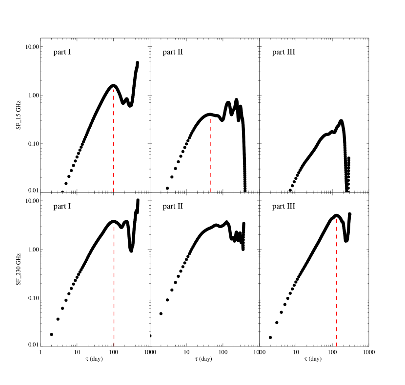
Figure 4: Structure function of S5 0716+714 for the parts I, II, and III of the 15 GHz (top) and 230 GHz (bottom) light curves.

Guided by the apparent different flaring behaviors during the observations, we first divided the light curves into three parts: part I for 2012.97-2014.22, including two major flares and a monotonic decaying, part II for 2014.22-2015.34, including several small but rapid flux enhancements, and part III for 2015.43-2016.12, covering the remaining light curves. The observed light curves were linearly interpolated for searching for clear peaks in the SF curves. The SF curves for each part at 15 and 230 GHz are shown in Figure 4. For both light curves, the SF curve shows a steep rising trend from the shortest time scale and a peak or plateau at the end of the rising trend, corresponding to a typical time scale of the variability in the light curves.

For part I covering the major flares, the SF curves show a steep rising trend with the first peak at the typical time scales of 100 and 103 days (errors are the mean cadence of data points) for 15 and 230 GHz light curves, respectively, suggesting that the major flares observed at different frequencies can be attributed to a common emission mechanism. The typical time scales are similar to those reported by Rani et al. (2013). The corresponding SF values at the peak are 1.6 and 3.8 for the 15 and 230 GHz, respectively. Because the SF value is proportional to the amplitude of the variability (e.g., Rani et al., 2013), for the major flare in part I, the amplitude of the variability in the flares is greater at the 230 GHz than at 15 GHz. For parts II and III covering the minor flux enhancements (15 GHz) and the major flare (230 GHz), the SF curves show a steep rising trend similar to that of part I, but the peaks in the SF curves of part III at 15 GHz and part II at 230 GHz are not clear. The first peaks in the SF curves of part II at 15 GHz and part III at 230 GHz, however, are clear with typical time scales of 43 and 130 days, respectively. The corresponding SF values at the peak are 0.4 and 5.0 for 15 and 230 GHz, respectively, implying that there are small but rapid flux enhancements as well as large and slow flares for parts II and III. Some physical parameters from the variability time scale are described in Section 3.3.

In order to quantify the amplitude of the variability of the 15 GHz and 230 GHz light curves, we estimated the modulation index $m$ following Kraus et al. (2003) as $m[\%]=100\sigma_{s}/\bar{S}$ where $\sigma_{s}$ and $\bar{S}$ represent the standard deviation and mean of the flux density $S$, respectively. The values of $m$ are 24 % at 15 GHz and 45 % at 230 GHz, indicating that S5 0716+714 shows relatively strong variation at 230 GHz as compared to that at 15 GHz.

3.3 Physical parameters from the variability time scale

3.3.1 Apparent brightness temperature from variability timescale

Assuming that the flux density variability is intrinsic to the source, the time scale of the variability constrains the size of the emitting region using causality argument. If the variable component is spherical with Gaussian brightness distribution, we can estimate the brightness temperature using the time scale of the variability as (Rani et al., 2013; Fuhrmann et al., 2008)

$$T^{app}_{B}=3.47\times{10}^{5}\cdot\Delta S\left(\frac{\lambda D_{L}}{\tau_{var}(1+z)^{2}}\right)^{2},$$ (2)

where $\Delta S$ is change of the flux density over time, $\tau_{var}$ is the variability time scale in year, which was obtained from the structure function in Section 3.2, $\lambda$ is the observing wavelength in cm, $D_{L}$ is the luminosity distance in Mpc, and z is the redshift. Here we used $D_{L}$=1510 Mpc (Fuhrmann et al., 2008), z=0.127 (Stadnik & Romani, 2014). The values of $\Delta S$ are listed in Table 3. The computed apparent brightness temperatures are $10^{13.8-14.5}$ K at 15 GHz, increasing by a factor of $\sim$4 from Part I to Part II, and $10^{11.5-11.7}$ K at 230 GHz, decreasing by a factor of $\sim$2 from Part I to Part III, as listed in Table 3. These values at 15 GHz are similar to those obtained by Rani et al. (2013).

3.3.2 Doppler factor

We estimated the high apparent brightness temperatures from the variability time scale exceeding inverse Compton (IC) limit of $T_{B}\sim 10^{12}$ K (Kellermann & Pauliny-Toth, 1969) at 15 GHz. Assuming that the excessive apparent brightness temperature is caused by relativistic boosting effect of the radiation, we can estimate Doppler factor:

$$\delta_{var}=(1+z)\left(\frac{T^{app}_{B}}{10^{12}}\right)^{1/(3+\alpha)}$$ (3)

where $\alpha$ is the spectral index of optically thin emission region (e.g., 86-129 GHz) and $\alpha$=-0.7 was adopted from the mean spectral index between 86 GHz and 129 GHz. The calculated Doppler factors are 7-13 at 15 GHz, increasing from Part I to Part II, and 0.6-0.8 at 230 GHz, being similar for Part I and III, as listed in Table 3. One possibility is that the emitting regions probed at 15 and 230 GHz may be different. If this is the case, it can be reasonable that the Doppler factor may not be the same in these regions. This may also explain the different $T_{B}$ and similar $\tau_{var}$, whilst smaller $\tau_{var}$ would normally be expected for higher frequencies (Rani et al., 2013).

3.3.3 Size of emitting region

Assuming again that the variability of the flux density is intrinsic to the source, the size of the emitting region $\theta$ [mas] can be calculated using the Doppler factor and variability time scale (see e.g., Fuhrmann et al., 2008, for details):

$$\theta=0.173\frac{\tau_{var}}{d_{L}}\delta_{var}(1+z),$$ (4)

where $\delta$ is Doppler factor and $\tau_{var}$ is the time scale of the variability in days. We obtained the size of emitting region of 0.07-0.09 at 15 GHz and 0.01 at 230 GHz which is listed in Table 3. The obtained size of emitting region at 15 GHz decreases by $\sim$20 % from Part I to Part II, and the size at 230 GHz is similar in Part I and Part III. The core sizes estimated by the variability time scales are much smaller (up to a factor of 10, for the case of 230 GHz) than the ones extrapolated from the measured model fitting sizes from the KVN data (see Table 2). This may be due to the fact that the KVN observations may be affected by an instrumental beam blending effect (making the observed core size larger than the true size) as discussed in Section 4.2.

3.4 Cross-correlation analysis at 15 and 230 GHz

In order to investigate a possible correlation and its corresponding time delay between the different wavelengths, we selected the 15 and 230 GHz light curves which are better sampled than the others. We calculated a cross-correlation analysis based on the discrete cross-correlation function (DCF) defined by Edelson & Krolik (1988) as follows:

$$UDCF_{ij}=\frac{(a_{i}-\bar{a})(b_{j}-\bar{b})}{\sqrt{\sigma^{2}_{a}-\sigma^{2}_{b}}},$$ (5)

where $a_{i}$ and $b_{j}$ are the measurements of data sets $a$ and $b$ for each light curve, $\bar{a}$ and $\bar{b}$ are the means of the data sets, and $\sigma_{a}$ and $\sigma_{b}$ are their corresponding standard deviations of the time series. The UDCF is binned with an interval $\Delta\tau$ for estimating the DCF

$$DCF(\tau)=\frac{1}{M}\sum{UDCF_{ij}(\tau)}$$ (6)

for each time lag, where $M$ is the number of data points in the bin. We estimated the standard error for each bin with the following equation:

$$\sigma_{DCF}(\tau)=\frac{1}{M-1}\sqrt{\sum[UDCF_{ij}(\tau)-DCF(\tau)]^{2}}.$$ (7)

To calculate the DCF, we used binning intervals of 2.2 days, 4.95 days, 4.3 days, and 3.25 days in part I, II, III, and entire period, respectively, which are half the mean cadence of each part, as shown in Figure 5. One expects to see a peak in the DCF curve for correlated variations, and the DCF peak time corresponds to the time delay between the two light curves. The uncertainty of the time lag was determined using a model-independent Monte Carlo method (e.g., see Peterson et al., 1998). We generated 1000 subsets which were randomly sampled from the light curves, and calculated a DCF analysis of the subsets, determining the time lags from N=1000 simulations. Based on 1000 time lags, we obtained a cross-correlation peak distribution (CCPD), as shown in the right panels of each plot in Figure 5. When the distribution of the CCPD is assumed to be a normal distribution, confidence interval of 95 %, $\Delta\tau_{95\%}$, can be computed from $\tau-1.96\frac{\sigma}{\sqrt{N}}<$ $\tau_{95\,\%}$ $<\tau+1.96\frac{\sigma}{\sqrt{N}}$. Here, N is number of simulation, $\tau$ is time lag with negative values meaning 230 GHz leads, and $\sigma$ is standard deviation of the CCPD. The values of $\tau$ are -17.36 days, -13.80 days, 44.49 days, and -15.88 days in part I, II, III, and entire period, respectively. The values of $\sigma$ are 4 in part I, 5 in part II, 44 in part III, and 8 days in entire period. The confidence interval for the part I is -17.59 $<\tau_{95\,\%}<$ -17.12, for the part II is -14.14 $<\tau_{95\,\%}<$ -13.46, and for the part III is 42.79 $<\tau_{95\,\%}<$ 46.19 for the entire period is -16.38 $<\tau_{95\,\%}<$ -15.38.

The time lag between 15 and 230 GHz for the entire period of the light curves is $-16\pm 8$ days (top left panel in Figure 5), implying that the 230 GHz light curve leads the 15 GHz light curve. For part I of the light curves, the time lag is also $-17\pm 4$ days, similar to the time differences of 20 days estimated above for the peaks in the light curves at 15 and 230 GHz (see 3.1.2), confirming that the 230 GHz light curve leads the 15 GHz light curve for major flares. The DCF time lag for part II is $-14\pm 5$ days, close to the time differences of 17 days for the peaks in the 15 and 230 GHz light curves (as discussed in Section 3.1.2), indicating that the 230 GHz light curve also leads the 15 GHz light curve for small flux enhancements. In this part, the multiple peaks of the DCF seem to be caused by correlation with the consecutive flares. Contrary to parts I and II, for part III, the determined time lag is $44\pm 27$ days. This result appears artificial because there is no well sampled measurement for the beginning portion of part III in the 230 GHz light curve and hence no corresponding measurements of the flux enhancements in the 15 GHz light curve.

In summary, the flares in the 230 GHz light curves lead those of the 15 GHz light curve with a time lag of $-14\sim-17$ days, except for part III. The time lag between flux enhancements at multi-frequency can be regarded by the opacity effect in the core region. Therefore, the postion of the VLBI core at 15 GHz with respect to 230 GHz can be drived by using the relation of $r_{core}=\mu\cdot\tau$ (Kudryavtseva et al., 2011). $\mu$ and $\tau$ correspond proper motion of the source in mas yr^-1 and the time lag derived from the DCF in year, respectively. Here, we adopted $\mu$=2.258 mas yr^-1 (Lister et al., 2016) and derived $r_{core}=0.09-0.1$ mas. This value shows a good agreement with a core position of $r_{core}=0.10\pm 0.03$ mas between 15 and 43 GHz measured from the VLBI by Martí-Vidal et al. (2016).

3.5 Brightness temperature

Brightness temperatures of the VLBI cores obtained from our VLBI measurements vary in time as shown in Figure 6 and summarized in Table 2. The observed brightness temperatures are in the ranges of $10^{8.3-10.3}$ K, $10^{9-10.8}$ K, $10^{9.2-10.6}$ K, and $10^{9.1-10.6}$ K at 22, 43, 86, and 129 GHz, respectively, including the lower limits of the brightness temperature, which were obtained for the unresolved cores (see Section 2.3). The mean brightness temperatures are $10^{8.8}$ K at 22 GHz, $10^{9.7}$ K at 43 GHz, $10^{10.1}$ K at 86 GHz, and $10^{10.2}$ K at 129 GHz, excluding the lower limits of the brightness temperatures, implying that the observed core brightness temperatures of S5 0716+714 become higher at higher frequency.

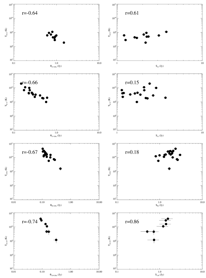
Figure 7: Brightness temperature as a function of deconvolved core size (left panels) and CLEAN flux density (right panels) for the different observing frequencies. The Pearson coefficient for a potential correlation is shown at each panel at the upper, left corner.

The observed brightness temperatures are lower than those obtained with the Very Long Baseline Array at 43 and 86 GHz by factors of about 10-200 (Hodgson, 2015), and with the Global Millimeter VLBI Array at 86 GHz by factors of about 4-20 (Lee et al., 2008). These results are also lower than the brightness temperature derived from the source variability at 86 GHz by orders of up to a factor of 3 (Rani et al., 2013). The difference may be due to the spatial resolution difference between the KVN and the global VLBI arrays, and to the instrumental beam blending effect (making the observed core size larger than the true size) as discussed in Section 4.2 and Lee et al. (2016b). The observed brightness temperatures are strongly correlated with the observed core size with correlation coefficient $r$ up to -0.74, whereas those are not with the CLEAN flux density with $r$ as small as 0.15 as shown in Figure 7, implying that the instrumental beam blending effect may play an important role in the brightness temperature estimation.

3.6 Spectral index

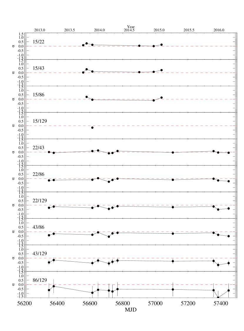
Figure 8: Multiwavelengths spectral indices of S5 0716+714.

Simultaneous multi-frequency observations with the KVN allow us to study the variation of the spectral index $\alpha$ ($S_{\nu}\propto\nu^{\alpha}$, where $\nu$ is the observing frequency, and $S_{\nu}$ is the flux density). In order to estimate the spectral index not only with KVN measurements but also with non-KVN measurements, we selected the non-KVN (i.e., OVRO) flux measurements when they were obtained closely to the KVN observations in time within one day (quasi-simultaneous). We found that there are six quasi-simultaneous flux measurements of OVRO, with regard to the KVN observations, as shown in Figure 8. In this figure, 1-${\sigma}$ error bars are plotted. The errors were estimated as

$$\sigma_{i,j}=\frac{\sqrt{(\sigma_{i}^{2}/S_{i}^{2})+(\sigma_{j}^{2}/S_{j}^{2})}}{\rm log(\nu_{i}/\nu_{j})}$$ (8)

where, $\sigma$, $S$, and $\nu$ are measurement error of the flux density, the flux density, and the observing frequency, respectively.

The spectral indices vary in time along $\alpha=0$ as summarized in Table 4. The spectral indices for most of the frequency pairs are $-0.5<\alpha<0.5$. For the 43-86 GHz, 43-129 GHz, and 86-129 GHz, the spectral index became steeper than $-$0.5, i.e., optically thin. The mean (and standard deviation) values of the spectral index are 0.13 (0.11) at 15-22 GHz, 0.16 (0.14) at 15-43 GHz, 0.06 (0.19) at 15-86 GHz, 0.06 (0.17) at 22-43 GHz, $-$0.09 (0.16) at 22-86 GHz, $-$0.27 (0.13) at 22-129 GHz, $-$0.25 (0.19) at 43-86 GHz, $-$0.44 (0.17) at 43-129 GHz, and $-$0.69 (0.32) at 86-129 GHz, indicating that the spectral index becomes steeper at pairs at higher frequencies.

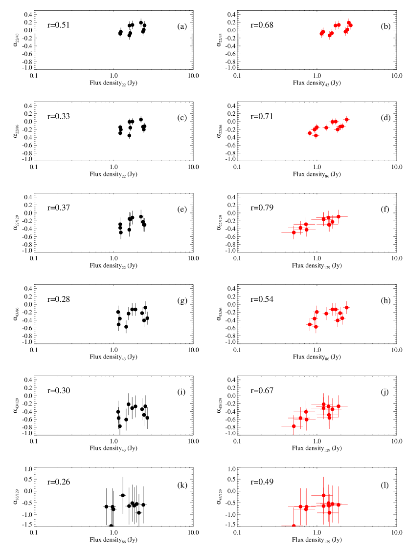
Figure 9: Spectral index at lower frequency (left panel) and at higher frequency (right panel) as a function of flux density for each pair of frequencies: (a)-(b) for 22-43 GHz, (c)-(d) for 22-86 GHz, (e)-(f) for 22-129 GHz, (g)-(h) for 43-86 GHz, (i)-(j) for 43-129 GHz, and (k)-(l) for 86-129 GHz. The Pearson coefficient for a potential correlation is shown at each panel at the upper, left corner.

By comparison of Figure 3 and 8, we see that the spectral indices follows similar trend to those of the observed flux densities. In order to investigate a correlation between the spectral indices and the flux densities of the observing frequencies, we estimated the Pearson correlation coefficient $r$. Figure 9 shows the spectral index as a function of the flux density at lower (left panels) and higher (right panels) frequency for 11 out of 29 epochs which yield the flux densities in all four frequency bands. Generally, the correlations between the spectral index and the flux density for each pair of frequencies are stronger (i.e., $r>0.5$) at a higher frequency, implying that the variation of the spectral index is more correlated with the flux density variation at a higher frequency than that at a lower frequency.

3.7 Source spectra

The simultaneous multi-frequency VLBI images obtained at four frequency bands (22, 43, 86, and 129 GHz) during such a long period of time are the first results for S5 0716+714, leading to the study of mas-scale spectral information without any uncertainty due to source variability. We used the CLEAN flux densities obtained on mas scales to investigate the spectral properties of the source.

Two models were used for fitting to the CLEAN flux density data: the power law and the curved power law, as given by

$$S\propto\nu^{+\alpha},$$ (9)

where $S$ is the CLEAN flux density in Jansky, $\nu$ is the observing frequency in GHz, $a$ is constant in Jansky, and $\alpha$ is the spectral index for the power law, and

$$S=c_{1}\left(\frac{\nu}{\nu_{\rm r}}\right)^{\alpha+c_{2}{\rm ln}(\nu/\nu_{\rm r})},$$ (10)

where $c_{1}$ (in Jansky) and $c_{2}$ are constant, $\nu_{\rm r}$ is a reference frequency, and $\alpha$ is the spectral index at $\nu_{\rm r}$.

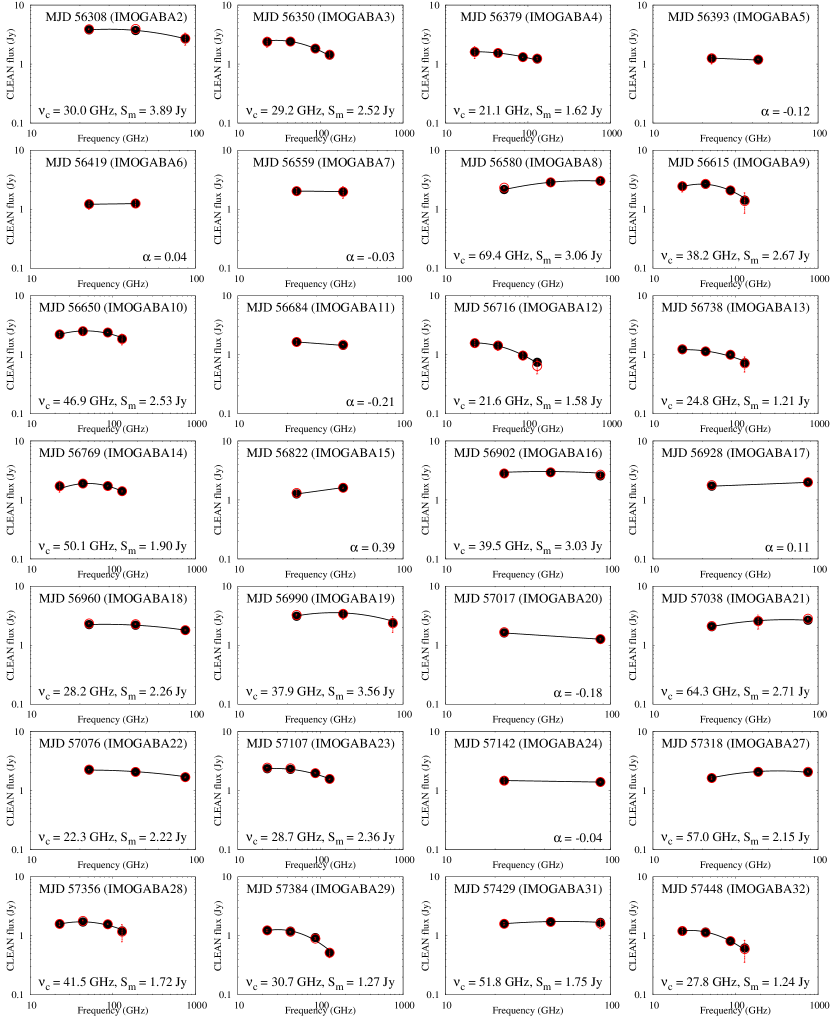
Figure 10: Spectra of CLEAN flux density (black dot) and core flux density (red circle) at 22-129 GHz for 28 epochs. Black solid lines are the best fitting power law.

Initially, the power law is fitted to the data. When the power law does not fit well the data due to the spectral curvature, a curved power law is used. For 8 out of 28 epochs, the power law was fitted to CLEAN flux measurements which were obtained at only two frequencies. The curved power law was well fitted to the CLEAN flux measurements for the remaining 20 epochs when the CLEAN flux measurements were available at more than three frequencies. We determined the peak flux density and turnover frequency by fitting the curved power-law with $\alpha=0$. The CLEAN flux spectra of 28 epochs are shown in Figure 10 with their best-fit model and fit parameters in table 5. Shown are the spectral index $\alpha$ for the power law, and the turnover frequency $\nu_{\rm c}$ and peak flux density $S_{\rm m}$ at $\nu_{\rm c}$ obtained from the curved power law.

4 Discussion

4.1 Turnover frequency

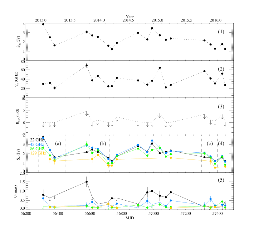
Figure 11: Variation of the peak flux densities (1), turnover frequencies (2), magnetic fields (3), KVN flux densities (4), and deconvolved core sizes (5) in the time domain.

From the spectral model fitting, we were able to obtain $\nu_{\rm c}$ and $S_{\rm m}$ for 20 epochs, as summarized in Table 5 and as shown in panels (1) and (2) of Figure 11, where we plot $S_{\rm m}$ and $\nu_{c}$ as a function of the observing time in order to investigate the variation of $\nu_{\rm c}$ and $S_{\rm m}$ in the time domain. We performed a Monte Carlo simulation with generating N=1000 spectra to obtain statistically meaningful values for the turnover frequency and the peak flux density as well as their uncertainties (see e.g. Fromm, 2015). $\nu_{\rm c}$ is in the range of 21 GHz-69 GHz with a mean turnover frequency $\bar{\nu}_{\rm c}$ of 37.7 GHz. The standard deviation of the turnover frequency $\sigma_{\nu_{\rm c}}$ is 14 GHz. $S_{\rm m}$ ranges from 1.21 Jy to 3.89 Jy with a mean peak flux density $\bar{S}_{m}$ of 2.3 Jy and corresponding standard deviation $\sigma_{S_{\rm m}}$ of 0.74 Jy. It is apparent that $S_{\rm m}$ and $S_{\nu}$ are correlated each other as well as with the KVN light curves.

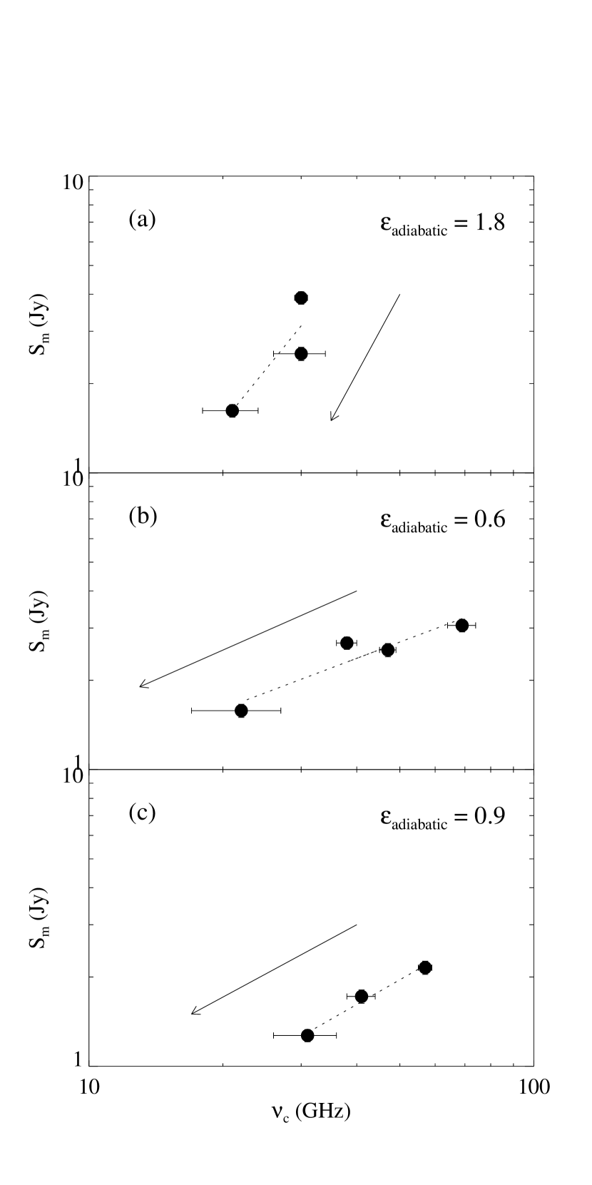
Figure 12: Evolution of the peak flux density $S_{\rm m}$ and the turnover frequency $\nu_{\rm c}$ for periods (a), (b), and (c). The arrows show the time flow in each period.

In order to study the evolution of the spectra over the time, we selected three periods of time in the KVN light curves: period (a) for 2013.04-2013.24, period (b) for 2013.79-2014.16, and period (c) is 2015.81-2015.99, which are relatively well sampled periods and which show a decaying trend. Figure 12 shows the evolution of the peak flux density $S_{\rm m}$ and the turnover frequency $\nu_{\rm m}$ for periods (a), (b), and (c). In this case, $S_{\rm m}$ increases as $S_{\rm m}\propto\nu_{\rm m}^{\epsilon_{\rm adiabatic}}$ with $\epsilon_{\rm adiabatic}=1.8$ for period (a), $\epsilon_{\rm adiabatic}=0.6$ for period (b), and $\epsilon_{\rm adiabatic}=0.9$ for period (c), which is consistent to the adiabatic stage (e.g., $\epsilon_{\rm adiabatic}=0.69$ in Marscher & Gear (1985) $\epsilon_{\rm adiabatic}=0.77$ in Fromm et al. (2011), and $\epsilon_{\rm adiabatic}=2$ for R8 flare of S5 0716+714 in Rani et al. (2013)) in the spectral evolution model of Marscher & Gear (1985), who discuss the evolution of a propagating shock wave in a steady state jet (or the shock-in-jet model). This may indicate that the flares are produced by a shock in the relativistic jet of S5 0716+714.

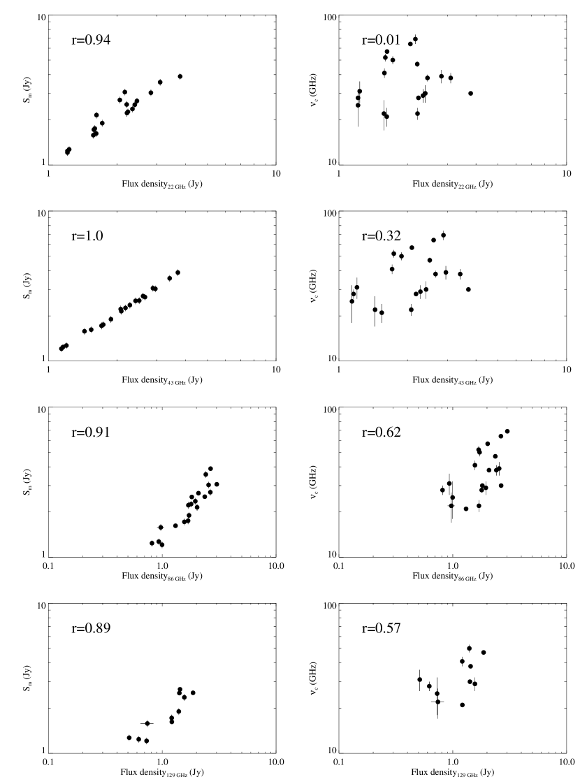
Figure 13: Peak flux density (left panels) and turnover frequency (right panels) as a function of the flux density for the different observing frequencies. The Pearson coefficient for a potential correlation is shown at each panel at the upper, left corner.

The correlations of the flux density at observing frequencies $S_{\nu}$ with $S_{\rm m}$ and $\nu_{\rm c}$ were investigated using the estimated linear correlation coefficient $r$, as shown in Figure 13. The linear correlation coefficients $r$ between $S_{\nu}$ and $S_{\rm m}$ are 0.94 at 22 GHz, 1.0 at 43 GHz, 0.91 at 86 GHz and 0.89 at 129 GHz, indicating that the peak flux density is strongly correlated with the flux density and shows the best correlation with the 43 GHz flux density. The linear correlation coefficients $r$ between $S_{\nu}$ and $\nu_{\rm c}$ are 0.01 at 22 GHz, 0.32 at 43 GHz, 0.62 at 86 GHz and 0.57 at 129 GHz, suggesting that the turnover frequency is less correlated with the flux density than with the peak flux density. The turnover frequency is most strongly correlated with the flux density at 86 GHz, indicating that the variation of the emission in optically thin region is very closely related to the change in the physical properties of synchrotron self-absorption.

4.2 Deconvolved core size

We obtained the core sizes deconvolved from the synthesized beams of KVN using a two-dimensional Gaussian model-fit, as summarized in Table 1. The ranges of the deconvolved core sizes are 0.1-1.5 mas at 22 GHz, 0.09-0.6 mas at 43 GHz, 0.09-0.4 mas at 86 GHz, and 0.09-0.3 mas at 129 GHz, including the upper limits of the size (the downward arrows in panel (5) in Figure 11). The mean (standard deviation) values of the deconvolved core sizes are 0.9 (0.2) mas, 0.3 (0.1) mas, 0.16 (0.08) mas, and 0.15 (0.07) mas at 22, 43, 86, and 129 GHz, respectively, excluding the upper limits of the size.

The deconvolved core sizes at 22 GHz and 43 GHz from the iMOGABA observations are $\sim$10 times larger than those from the VLBA observations at 22 GHz (Bach et al., 2005, $\theta\sim 0.1$ mas) and at 43 GHz (Rani et al., 2015, $\theta\sim 0.04$ mas), respectively, for S5 0716+714. This is mainly attributed to the relatively large synthesized beams of the KVN (6 mas at 22 GHz and 3 mas at 43 GHz) as compared to those of the VLBA (0.3 mas at 22 GHz and 0.15 mas at 43 GHz), which may lead to an instrumental beam blending effects: the deconvolved core region is diluted by jet emissions coming from regions downstream of the $\tau=1$ surface (Lee et al., 2016b).

As shown in panel (5) of Figure 11, the deconvolved core size was found to vary in time, which may be due to several factors, such as (a) errors when deconvolving the core with two-dimensional Gaussian models, (b) the variation of the viewing angle of the core emission region, (c) the ejection of a new jet component still located in the blended core.

The fitting errors are 0.010 mas at 22 GHz, 0.016 mas at 43 GHz, 0.020 mas at 86 GHz, and 0.024 mas at 129 GHz, which are much smaller than the standard deviations (0.07-0.2 mas) of the deconvolved core sizes at 22, 43, and 86 GHz, ruling out fitting errors due to time variations of the core size. The variation of the viewing angle from $\psi_{1}$ to $\psi_{2}$ may cause a fractional change of the deconvolved core size via $|\Delta d|/d=|cos\psi_{2}-cos\psi_{1}|$ which may be at most 0.015 (1.5 %) for a large change of the viewing angle from $\psi_{1}\sim 1^{\circ}$ to $\psi_{2}\sim 10^{\circ}$, as reported in Rani et al. (2015). This value is much smaller than the fractional change (20 %-50 %) of the deconvolved core size obtained from the iMOGABA observations.

In the case of the ejection of a new jet component, the variation of the deconvolved core size may depend on the jet angular speed $\mu$. The mean angular speed $\bar{\mu}$ of new jet components of S5 0716+714 is as large as $\mu\sim$1 mas yr^-1 (see Rani et al., 2015). When a new jet component emerges from the core region and is blended with the core, the blended core size $d$ may increase as $\Delta d\propto\mu$. If the new jet component is resolved from the core, the deconvolved core size may rapidly decrease. The standard deviations of the deconvolved core sizes in the iMOGABA observations are larger than 0.1 mas (at 22, 43, and 86 GHz), corresponding to the angular movement of the new jet component of S5 0716+714 in one month (i.e., the observing cadence of the iMOGABA). Therefore, the time variation in the deconvolved core size may be partly attributed to the instrumental beam blending effect and a newly ejected jet component still located in the blended core region. We may find, for example,that the deconvolved core size increases from 0.1 mas to 0.4 mas at 86 GHz during 2015.91-2016.11 (i.e., $\Delta d\sim 1.6$ mas yr^-1).

4.3 Magnetic field

The turnover frequency $\nu_{c}$ and peak flux density $S_{\rm m}$ determined by the spectral model fitting (see Section 4.1) enable us to constrain the magnetic field in the emission region dominating the flux density at the turnover frequency, assuming that the emission region is a compact and hence homogeneous synchrotron self-absorption (SSA) region, following Marscher (1983) and Hodgson et al. (2017) as

$$B=10^{-5}b(\alpha)S^{-2}_{\rm m}\theta^{4}\nu_{c}^{5}\left(\frac{\delta}{1+z}\right)^{-1}~{}~{}~{}(G),$$ (11)

where $b(\alpha)$ is a parameter which depends on optically thin spectral index ranging from 1.8 to 3.8 (see Table 1 in Marscher, 1983), $S_{\rm m}$ is the peak flux density in Jy, $\theta$ is the angular size (mas) of the emission region, $\nu_{\rm c}$ is the turnover frequency in GHz, $\delta$ is the Doppler factor, and $z$ denotes the redshift. We should note that Equation (11) is updated from that in Marscher (1983) with the $\left(\frac{\delta}{1+z}\right)$ factor being raised to the $-1$ power rather than $+1$ power, since the VLBI core of this source is in a steady state rather than evolving in time (A. Marscher, private communication).

Given that the deconvolved core size from the iMOGABA observations may include the instrumental beam blending effect, we used $\theta=0.04$ mas obtained from the VLBI observations, and assumed $\delta=7$, following Rani et al. (2013). Using $b(\alpha)$ = 2.92, $S_{\rm m}$ = 1.2-3.9 Jy, and $\nu_{\rm c}$ = 21.1-69.4 GHz, we obtained the upper limits of the magnetic field $B$ of $\leq 5$ mG during the observing period, as summarized in Table 5, yielding a weighted mean of $1.0\pm 0.6$ mG for higher turnover frequencies (e.g., $>$45 GHz). This result is consistent with those in Rani et al. (2013) when applying equation (11).

5 Summary

Three years of multi-frequency VLBI monitoring observations of S5 0716+714 using KVN at 22, 43, 86, and 129 GHz, together with 15 and 230 GHz total intensity data, enabled us to find the following conclusions:

• S5 0716+714 is compact on the mas scale at 22-129 GHz under the KVN resolution, showing only a VLBI core component. During the observing period of time, there were several major flares with peak flux densities of $\sim$4 Jy at 15 GHz and $\sim$7 Jy at 230 GHz.

• The typical time scales of the flares are 43-100 days at 15 GHz and 100-130 days at 230 GHz. The 230 GHz light curve leads the 15 GHz one with a time-lag of -16$\pm$8 days for these flares.

• The two-frequency spectral indices are in the range of -0.5 to 0.5 and are steeper at higher frequency pairs with $\alpha\leq-1.5$. The variation in the two-frequency spectral index is more correlated with the flux density at a higher frequency, i.e., in the case of optically thin emission.

• The spectrum of the source obtained from the simultaneous multifrequency VLBI observations at 22-129 GHz has a spectral break (i.e., turnover frequency) and varies in time. The turnover frequency varies from 21 GHz to 69 GHz with its peak flux density ranging from 1 Jy to 4 Jy.

• The evolution of the turnover frequency and the peak flux density can be well described by the shock-in-jet model (Marscher & Gear, 1985), especially as an adiabatic stage during the decreasing phase of the flux density.

• The deconvolved core sizes obtained from the two-dimensional Gaussian modelfit are $\sim$10 times larger at 22 and 43 GHz than previous VLBI measurements (e.g., Bach et al., 2005; Rani et al., 2015) mainly due to instrumental beam blending effects. We partially explain the time variation of the deconvolved core size (e.g., at 86 GHz) by the ejection of new jet components.

• By assuming a synchrotron self-absorption model for the relativistic jet emission in S5 0716+714, we estimated the magnetic field strength in the mas emission region to be $\leq 5$ mG during the observing period, yielding a weighted mean of $1.0\pm 0.6$ mG for higher turnover frequencies (e.g., $>$45 GHz).

Figure 1: The distribution of the image quality factor $\xi_{\rm r}$ (ratio of the image root-mean-square noise to its mathematical expectation). The mean and range of the distribution are presented.

Figure 2: Example of contour map (upper left), residual map (lower left), the visibility amplitude against uv-radius (upper right), and the closure phase as function of time (lower right), at 129 GHz band obtained in March 28, 2013 (MJD 56379)

Figure 3: Light curves of S5 0716+714 from radio to mm wavelength observed during 2013.04-2016.16.

Figure 5: Cross-correlation functions and the corresponding cross-correlation peak distributions (CCPD) of the light curves at 15 and 230 GHz in S5 0716+714 for the entire period (top left), part I (top right), part II (bottom left), and part III (bottom right), and the corresponding cross-correlation peak distributions (CCPD).

Figure 6: Brightness temperatures of the VLBI core of S5 0716+714 observed in the 22 GHz, 43 GHz, 86 GHz, and 129 GHz bands, from top to bottom. Arrows indicate the lower limits.

Table 1: Image parameters

Epoch	MJD	Band	$B_{\rm maj}$	$B_{\rm min}$	$B_{\rm PA}$	$S_{\rm KVN}$	$S_{\rm p}$	$\sigma$	$D$	$\xi_{\rm r}$
(1)	(2)	(3)	(4)	(5)	(6)	(7)	(8)	(9)	(10)	(11)
2013 Jan 16	56308	K	5.471	4.052	$-$86.4	3.791	3.787	16	234	0.61
		Q	2.723	2.030	$-$85.7	3.705	3.703	29	129	0.62
		W	1.354	0.914	89.3	2.660	2.694	74	36	0.41
2013 Feb 27	56350	K	5.509	4.173	$-$72.8	2.396	2.409	10	251	0.58
		Q	2.692	2.055	$-$76.5	2.415	2.399	28	86	0.59
		W	1.317	1.044	89.4	1.819	1.804	66	27	0.57
		D	0.920	0.701	$-$56.7	1.415	1.418	63	23	0.59
2013 Mar 28	56379	K	5.373	4.585	$-$64.7	1.622	1.623	5	359	0.67
		Q	2.735	2.319	$-$61.0	1.542	1.543	11	142	0.69
		W	1.308	1.093	$-$77.2	1.309	1.298	25	51	0.59
		D	0.889	0.610	$-$79.5	1.215	1.191	57	21	0.56
2013 Apr 11	56393	K	5.330	4.294	$-$79.0	1.262	1.261	6	200	0.59
		Q	2.703	2.055	$-$80.2	1.170	1.173	20	59	0.60
2013 May 07	56419	K	6.443	4.533	$-$48.4	1.219	1.237	7	173	0.54
		Q	3.291	2.241	$-$55.5	1.252	1.244	21	59	0.55
2013 Sep 24	56559	K	5.514	4.145	$-$62.6	2.041	2.041	13	153	0.65
		Q	2.744	2.154	$-$57.7	2.000	2.007	27	74	0.54
2013 Oct 15	56580	K	5.663	4.634	$-$73.4	2.167	2.160	22	96	0.56
		Q	3.414	2.439	$-$45.2	2.879	2.864	41	70	0.49
		W	1.806	1.228	$-$29.7	3.016	3.006	126	24	0.47
2013 Nov 19	56615	K	5.849	4.196	$-$61.1	2.449	2.486	20	122	0.61
		Q	2.857	2.005	$-$70.4	2.657	2.634	20	131	0.62
		W	1.440	0.969	$-$73.9	2.082	2.077	28	73	0.53
		D	0.934	0.645	$-$63.0	1.434	1.427	31	46	0.57
2013 Dec 24	56650	K	5.741	4.258	$-$54.1	2.208	2.208	10	220	0.58
		Q	2.861	2.151	$-$57.3	2.506	2.507	13	190	0.62
		W	1.469	1.042	$-$51.3	2.365	2.357	23	103	0.55
		D	1.000	0.663	$-$51.9	1.866	1.868	29	64	0.58
2014 Jan 27	56684	K	5.880	4.459	$-$53.0	1.642	1.643	12	142	0.63
		Q	2.890	2.144	$-$57.1	1.433	1.453	22	65	0.54
2014 Feb 28	56716	K	6.768	3.519	$-$51.7	1.576	1.574	19	84	0.57
		Q	3.341	1.861	$-$46.4	1.441	1.434	27	54	0.57
		W	2.085	0.841	$-$43.8	0.971	0.968	69	14	0.57
		D	1.372	0.611	$-$36.3	0.741	0.604	96	6	0.45
2014 Mar 22	56738	K	5.273	3.800	$-$68.0	1.213	1.213	6	217	0.55
		Q	2.589	1.959	$-$68.2	1.141	1.129	12	92	0.61
		W	1.407	0.912	$-$61.8	0.997	0.987	22	45	0.58
		D	0.869	0.642	$-$74.3	0.729	0.712	24	29	0.68
2014 Apr 22	56769	K	5.274	3.775	$-$71.7	1.724	1.733	7	257	0.68
		Q	2.641	1.887	$-$69.1	1.883	1.859	18	106	0.69
		W	1.390	0.884	$-$79.4	1.720	1.706	32	54	0.63
		D	0.952	0.580	$-$79.1	1.398	1.383	28	49	0.54
2014 Jun 13	56822	K	5.330	4.294	$-$79.0	1.262	1.261	6	200	0.59
		Q	2.645	1.943	$-$68.8	1.621	1.585	33	49	0.62
2014 Sep 01	56902	K	5.346	3.692	$-$87.3	2.820	2.815	13	215	0.69
		Q	2.753	1.792	$-$83.1	2.950	2.939	20	145	0.56
		W	1.378	0.898	$-$88.8	2.556	2.550	31	83	0.55
2014 Sep 27	56928	K	5.723	3.474	$-$67.0	1.711	1.709	7	232	0.68
		W	1.544	0.805	$-$72.1	1.984	1.965	61	32	0.59
2014 Oct 29	56960	K	5.862	3.422	$-$74.4	2.235	2.233	12	190	0.66
		Q	2.904	1.739	$-$72.2	2.181	2.172	22	98	0.62
		W	1.636	0.799	$-$70.0	1.795	1.779	33	53	0.57
2014 Nov 28	56990	K	5.657	3.436	$-$71.8	3.097	3.089	24	128	0.63
		Q	2.761	1.770	$-$73.8	3.410	3.428	19	183	0.65
		W	1.467	0.834	$-$72.9	2.415	2.406	55	44	0.69
2014 Dec 25	57017	K	5.431	3.672	$-$72.3	1.613	1.610	9	183	0.67
		W	1.368	0.912	$-$69.2	1.265	1.249	28	45	0.60
2015 Jan 15	57038	K	6.055	3.358	$-$70.9	2.060	2.058	8	265	0.63
		Q	2.881	1.752	$-$72.4	2.606	2.603	11	228	0.70
		W	1.555	0.825	$-$70.3	2.648	2.636	28	93	0.65
2015 Feb 23	57076	K	5.360	3.747	$-$71.2	2.214	2.214	5	463	0.70
		Q	2.604	1.961	$-$72.7	2.078	2.051	20	105	0.57
		W	1.471	0.971	$-$53.6	1.698	1.665	72	23	0.49
2015 Mar 26	57107	K	5.400	3.626	$-$80.5	2.340	2.336	7	353	0.60
		Q	2.599	1.907	$-$76.5	2.280	2.272	7	339	0.62
		W	1.364	0.899	$-$80.9	1.953	1.939	29	67	0.67
		D	0.900	0.621	$-$75.8	1.565	1.550	41	38	0.54
2015 Apr 30	57142	K	5.452	3.729	$-$71.8	1.476	1.475	13	118	0.71
		W	1.440	0.862	$-$73.5	1.390	1.373	26	53	0.67
2015 Oct 23	57318	K	5.647	3.843	$-$66.8	1.627	1.626	14	112	0.63
		Q	2.950	1.895	$-$58.9	2.091	2.049	41	50	0.53
		W	1.636	0.912	$-$53.1	2.026	2.021	82	25	0.49
2015 Nov 30	57356	K	5.398	3.773	$-$71.8	1.584	1.585	9	169	0.58
		Q	2.738	1.841	$-$67.4	1.712	1.679	10	175	0.53
		W	1.451	0.883	$-$68.2	1.566	1.555	18	88	0.64
		D	0.956	0.598	$-$68.5	1.211	1.206	24	49	0.55
2015 Dec 28	57384	K	5.327	3.781	$-$68.2	1.234	1.234	8	155	0.62
		Q	2.647	1.950	$-$68.5	1.200	1.161	6	204	0.79
		W	1.415	0.906	$-$68.6	0.933	0.880	12	71	0.66
		D	0.922	0.625	$-$64.5	0.513	0.508	10	50	0.71
2016 Jan 13	57400	K	5.310	3.952	$-$66.1	1.261	1.260	5	240	0.74
2016 Feb 11	57429	K	5.548	4.153	$-$82.2	1.599	1.598	9	177	0.63
		Q	2.863	2.086	$-$73.9	1.742	1.698	17	103	0.69
		W	1.557	0.990	$-$73.5	1.688	1.482	44	34	0.65
2016 Mar 01	57448	K	5.250	3.856	$-$66.6	1.213	1.213	5	222	0.63
		Q	2.609	1.964	$-$66.9	1.159	1.125	6	193	0.65
		W	1.350	0.935	$-$68.5	0.813	0.805	9	92	0.70
		D	0.868	0.669	$-$57.5	0.622	0.620	9	67	0.60

Note. — Column designation: 1 - Date; 2 - modified Julian date; 3 - observing frequency band: K - 22 GHz band; Q - 43 GHz band; W - 86 GHz band; D - 129 GHz band; 4-6 - restoring beam: 4 - major axis [mas]; 5 - minor axis [mas]; 6 - position angle of the major axis [degree]; 7 - total cleaned KVN flux density [Jy]; 8 - peak flux density [Jy beam^-1]; 9 - off-source RMS in the image [Jy beam^-1]; 10 - dynamic range of the image; 11 - quality of the residual noise in the image (i.e., ratio of the image root-mean-square noise to its mathematical expectation).

Table 2: Modelfit parameters

Epoch	MJD	Band	$S_{\rm tot}$	$S_{\rm peak}$	$d$	$r$	$\theta$	$T_{\rm b}$
(1)	(2)	(3)	(4)	(5)	(6)	(7)	(8)	(9)
2013 Jan 16	56308	K	3.89$\pm$ 0.04	3.79$\pm$ 0.03	0.80$\pm$ 0.01	…	…	1.12$\pm$ 0.02
		Q	3.93$\pm$ 0.06	3.70$\pm$ 0.04	0.60$\pm$ 0.01	…	…	1.99$\pm$ 0.04
		W	2.72$\pm$ 0.63	2.62$\pm$ 0.44	$<$0.17	…	…	$>$17.74
2013 Feb 27	56350	K	2.39$\pm$ 0.47	2.41$\pm$ 0.33	$<$0.63	…	…	$>$1.13
		Q	2.41$\pm$ 0.02	2.40$\pm$ 0.02	0.15$\pm$ 0.00	…	…	20.08$\pm$ 0.27
		W	1.83$\pm$ 0.05	1.80$\pm$ 0.03	0.14$\pm$ 0.00	…	…	16.11$\pm$ 0.62
		D	1.44$\pm$ 0.16	1.42$\pm$ 0.12	0.13$\pm$ 0.01	…	…	15.57$\pm$ 2.53
2013 Mar 28	56379	K	1.60$\pm$ 0.37	1.62$\pm$ 0.26	$<$0.75	…	…	$>$0.53
		Q	1.54$\pm$ 0.17	1.54$\pm$ 0.12	$<$0.19	…	…	$>$8.17
		W	1.31$\pm$ 0.02	1.30$\pm$ 0.02	0.13$\pm$ 0.00	…	…	15.05$\pm$ 0.38
		D	1.24$\pm$ 0.06	1.19$\pm$ 0.04	0.15$\pm$ 0.01	…	…	10.61$\pm$ 0.79
2013 Apr 11	56393	K	1.25$\pm$ 0.25	1.26$\pm$ 0.17	$<$0.63	…	…	$>$0.59
		Q	1.19$\pm$ 0.02	1.17$\pm$ 0.01	0.31$\pm$ 0.00	…	…	2.28$\pm$ 0.05
2013 May 07	56419	K	1.23$\pm$ 0.22	1.24$\pm$ 0.16	$<$0.66	…	…	$>$0.53
		Q	1.25$\pm$ 0.16	1.24$\pm$ 0.11	$<$0.22	…	…	$>$4.68
2013 Sep 24	56559	K	2.04$\pm$ 0.21	2.04$\pm$ 0.15	$<$0.33	…	…	$>$3.45
		Q	1.98$\pm$ 0.44	2.01$\pm$ 0.32	$<$0.36	…	…	$>$2.81
2013 Oct 15	56580	K	2.33$\pm$ 0.06	2.16$\pm$ 0.04	1.50$\pm$ 0.03	…	…	0.19$\pm$ 0.01
		Q	2.87$\pm$ 0.31	2.87$\pm$ 0.22	0.23$\pm$ 0.02	…	…	9.94$\pm$ 1.52
		W	3.04$\pm$ 0.30	3.01$\pm$ 0.21	0.20$\pm$ 0.01	…	…	14.65$\pm$ 2.05
2013 Nov 19	56615	K	2.46$\pm$ 0.50	2.49$\pm$ 0.36	$<$0.67	…	…	$>$1.01
		Q	2.70$\pm$ 0.01	2.63$\pm$ 0.01	0.41$\pm$ 0.00	…	…	2.92$\pm$ 0.02
		W	2.10$\pm$ 0.03	2.08$\pm$ 0.02	0.12$\pm$ 0.00	…	…	29.33$\pm$ 0.63
		D	1.38$\pm$ 0.53	1.43$\pm$ 0.38	$<$0.20	…	…	$>$6.63
2013 Dec 24	56650	K	2.20$\pm$ 0.20	2.21$\pm$ 0.14	$<$0.30	…	…	$>$4.65
		Q	2.50$\pm$ 0.30	2.51$\pm$ 0.21	$<$0.20	…	…	$>$12.11
		W	2.37$\pm$ 0.02	2.36$\pm$ 0.02	0.10$\pm$ 0.00	…	…	40.61$\pm$ 0.53
		D	1.84$\pm$ 0.39	1.87$\pm$ 0.27	$<$0.11	…	…	$>$26.68
2014 Jan 27	56684	K	1.64$\pm$ 0.15	1.64$\pm$ 0.10	$<$0.30	…	…	$>$3.32
		Q	1.47$\pm$ 0.02	1.45$\pm$ 0.02	0.28$\pm$ 0.00	…	…	3.40$\pm$ 0.07
2014 Feb 28	56716	K	1.57$\pm$ 0.20	1.57$\pm$ 0.14	$<$0.42	…	…	$>$1.66
		Q	1.42$\pm$ 0.25	1.44$\pm$ 0.18	$<$0.29	…	…	$>$3.17
		W	0.96$\pm$ 0.10	0.97$\pm$ 0.07	$<$0.09	…	…	$>$20.69
		D	0.64$\pm$ 0.17	0.58$\pm$ 0.11	0.31$\pm$ 0.06	…	…	1.24$\pm$ 0.49
2014 Mar 22	56738	K	1.23$\pm$ 0.01	1.21$\pm$ 0.01	0.61$\pm$ 0.00	…	…	0.62$\pm$ 0.01
		Q	1.14$\pm$ 0.01	1.13$\pm$ 0.01	0.17$\pm$ 0.00	…	…	6.94$\pm$ 0.12
		W	1.00$\pm$ 0.02	0.99$\pm$ 0.01	0.11$\pm$ 0.00	…	…	14.20$\pm$ 0.39
		D	0.71$\pm$ 0.20	0.71$\pm$ 0.14	0.17$\pm$ 0.03	…	…	4.56$\pm$ 1.86
2014 Apr 22	56769	K	1.71$\pm$ 0.36	1.73$\pm$ 0.26	$<$0.63	…	…	$>$0.80
		Q	1.89$\pm$ 0.04	1.86$\pm$ 0.03	0.33$\pm$ 0.00	…	…	3.32$\pm$ 0.09
		W	1.72$\pm$ 0.03	1.71$\pm$ 0.02	0.11$\pm$ 0.00	…	…	26.84$\pm$ 0.64
		D	1.41$\pm$ 0.03	1.38$\pm$ 0.02	0.09$\pm$ 0.00	…	…	29.46$\pm$ 1.02
2014 Jun 13	56822	K	1.31$\pm$ 0.14	1.26$\pm$ 0.10	0.92$\pm$ 0.07	…	…	0.29$\pm$ 0.05
		Q	1.60$\pm$ 0.03	1.58$\pm$ 0.02	0.27$\pm$ 0.00	…	…	3.96$\pm$ 0.11
2014 Sep 01	56902	K	2.81$\pm$ 0.29	2.81$\pm$ 0.20	$<$0.30	…	…	$>$5.63
		Q	2.94$\pm$ 0.19	2.94$\pm$ 0.13	$<$0.09	…	…	$>$61.14
		W	2.68$\pm$ 0.21	2.55$\pm$ 0.14	0.26$\pm$ 0.01	…	…	7.44$\pm$ 0.83
2014 Sep 27	56928	K	1.78$\pm$ 0.02	1.71$\pm$ 0.01	0.90$\pm$ 0.01	…	…	0.41$\pm$ 0.01
		W	1.99$\pm$ 0.05	1.97$\pm$ 0.03	0.12$\pm$ 0.00	…	…	23.62$\pm$ 0.77
2014 Oct 29	56960	K	2.33$\pm$ 0.03	2.23$\pm$ 0.02	0.93$\pm$ 0.01	…	…	0.50$\pm$ 0.01
		Q	2.27$\pm$ 0.03	2.17$\pm$ 0.02	0.47$\pm$ 0.01	…	…	1.92$\pm$ 0.04
		W	1.80$\pm$ 0.03	1.78$\pm$ 0.02	0.11$\pm$ 0.00	…	…	27.51$\pm$ 0.75
2014 Nov 28	56990	K	3.25$\pm$ 0.09	3.09$\pm$ 0.06	1.00$\pm$ 0.02	…	…	0.61$\pm$ 0.02
		Q	3.40$\pm$ 0.65	3.43$\pm$ 0.46	$<$0.28	…	…	$>$8.08
		W	2.35$\pm$ 0.71	2.41$\pm$ 0.51	$<$0.22	…	…	$>$8.93
2014 Dec 25	57017	K	1.66$\pm$ 0.03	1.61$\pm$ 0.02	0.83$\pm$ 0.01	…	…	0.45$\pm$ 0.01
		W	1.27$\pm$ 0.04	1.25$\pm$ 0.03	0.14$\pm$ 0.00	…	…	11.18$\pm$ 0.48
2015 Jan 15	57038	K	2.12$\pm$ 0.02	2.06$\pm$ 0.02	0.74$\pm$ 0.01	…	…	0.71$\pm$ 0.01
		Q	2.56$\pm$ 0.69	2.60$\pm$ 0.49	$<$0.40	…	…	$>$2.96
		W	2.81$\pm$ 0.06	2.64$\pm$ 0.04	0.28$\pm$ 0.00	…	…	6.73$\pm$ 0.21
2015 Feb 23	57076	K	2.26$\pm$ 0.02	2.21$\pm$ 0.01	0.67$\pm$ 0.00	…	…	0.93$\pm$ 0.01
		Q	2.06$\pm$ 0.02	2.05$\pm$ 0.01	0.18$\pm$ 0.00	…	…	11.17$\pm$ 0.14
		W	1.68$\pm$ 0.04	1.67$\pm$ 0.03	0.13$\pm$ 0.00	…	…	19.03$\pm$ 0.63
2015 Mar 26	57107	K	2.44$\pm$ 0.02	2.34$\pm$ 0.01	0.94$\pm$ 0.00	…	…	0.51$\pm$ 0.01
		Q	2.38$\pm$ 0.02	2.27$\pm$ 0.01	0.49$\pm$ 0.00	…	…	1.81$\pm$ 0.02
		W	1.97$\pm$ 0.04	1.94$\pm$ 0.03	0.14$\pm$ 0.00	…	…	19.13$\pm$ 0.54
		D	1.57$\pm$ 0.03	1.55$\pm$ 0.02	0.09$\pm$ 0.00	…	…	37.54$\pm$ 0.90
2015 Apr 30	57142	K	1.47$\pm$ 0.22	1.48$\pm$ 0.16	$<$0.45	…	…	$>$1.34
		W	1.39$\pm$ 0.03	1.38$\pm$ 0.02	0.13$\pm$ 0.00	…	…	15.74$\pm$ 0.44
2015 Oct 23	57318	K	1.63$\pm$ 0.07	1.63$\pm$ 0.05	$<$0.14	…	…	$>$16.01
		Q	2.07$\pm$ 0.03	2.05$\pm$ 0.02	0.24$\pm$ 0.00	…	…	6.82$\pm$ 0.15
		W	2.07$\pm$ 0.05	2.02$\pm$ 0.04	0.19$\pm$ 0.00	…	…	10.30$\pm$ 0.39
2015 Nov 30	57356	K	1.59$\pm$ 0.11	1.58$\pm$ 0.08	$<$0.20	…	…	$>$7.22
		Q	1.78$\pm$ 0.05	1.68$\pm$ 0.04	0.57$\pm$ 0.01	…	…	1.00$\pm$ 0.04
		W	1.57$\pm$ 0.02	1.56$\pm$ 0.02	0.11$\pm$ 0.00	…	…	25.86$\pm$ 0.57
		D	1.18$\pm$ 0.39	1.21$\pm$ 0.28	$<$0.17	…	…	$>$7.98
2015 Dec 28	57384	K	1.23$\pm$ 0.05	1.23$\pm$ 0.03	$<$0.11	…	…	$>$18.91
		Q	1.17$\pm$ 0.02	1.16$\pm$ 0.01	0.23$\pm$ 0.00	…	…	4.28$\pm$ 0.11
		W	0.90$\pm$ 0.03	0.88$\pm$ 0.02	0.17$\pm$ 0.00	…	…	5.75$\pm$ 0.28
		D	0.52$\pm$ 0.09	0.51$\pm$ 0.06	0.14$\pm$ 0.02	…	…	4.68$\pm$ 1.20
2016 Jan 13	57400	K	1.25$\pm$ 0.17	1.26$\pm$ 0.12	$<$0.40	…	…	$>$1.42
2016 Feb 11	57429	K	1.60$\pm$ 0.07	1.60$\pm$ 0.05	$<$0.15	…	…	$>$13.19
		Q	1.72$\pm$ 0.03	1.70$\pm$ 0.02	0.27$\pm$ 0.00	…	…	4.53$\pm$ 0.11
		W	1.62$\pm$ 0.31	1.46$\pm$ 0.21	0.44$\pm$ 0.06	…	…	1.56$\pm$ 0.44
2016 Mar 01	57448	K	1.21$\pm$ 0.18	1.21$\pm$ 0.13	$<$0.45	…	…	$>$1.09
		Q	1.13$\pm$ 0.02	1.12$\pm$ 0.01	0.23$\pm$ 0.00	…	…	4.11$\pm$ 0.09
		W	0.81$\pm$ 0.02	0.81$\pm$ 0.01	0.11$\pm$ 0.00	…	…	11.79$\pm$ 0.31
		D	0.60$\pm$ 0.24	0.62$\pm$ 0.17	$<$0.21	…	…	$>$2.62

Note. — Column designation: 1 - date; 2 - modified Julian date; 3 - observing frequency band: K - 22 GHz band; Q - 43 GHz band; W - 86 GHz band; D - 129 GHz band; 4 - model flux density of the component [Jy]; 5 - peak brightness of an individual component measured in the image [Jy beam^-1]; 6 - size [mas], italic numbers indicate upper limits; 7 - radius [mas]; 8 - position angle [deg]; 9 - measured brightness temperature [$10^{9}$ K], italic numbers indicate lower limits.

Table 3: Apparent brightness temperature, Doppler factor and size of emitting region

Part I

Part II

Part III

$\nu$

$\tau_{var}$

$\Delta S$

$T^{app}_{B}$

$\delta_{var}$

$\theta$

$\tau_{var}$

$\Delta S$

$T^{app}_{B}$

$\delta_{var}$

$\theta$

$\tau_{var}$

$\Delta S$

$T^{app}_{B}$

$\delta_{var}$

$\theta$

(GHz)

(days)

(Jy)

(K)

(mas)

(days)

(Jy)

(K)

(mas)

(days)

(Jy)

(K)

(mas)

15

100

2.5

7$\times 10^{13}$

6.9

0.09

43

1.8

3$\times 10^{14}$

12.5

0.07

—

230

103

4.5

5$\times 10^{11}$

0.8

0.01

—

130

4.3

3$\times 10^{11}$

0.6

0.01

Table 4: Spectral indices

Frequency	N	$\alpha$
15-22 GHz	6	0.01…0.3
15-43 GHz	6	0.02…0.38
15-86 GHz	4	$-$0.14…0.26
15-129 GHz	1	$-$0.22
22-43 GHz	25	$-$0.20…0.42
22-86 GHz	23	$-$0.36…0.24
22-129 GHz	11	$-$0.49…$-$0.10
43-86 GHz	20	$-$0.57…0.07
43-129 GHz	11	$-$0.77…$-$0.22
86-129 GHz	11	$-$1.5…$-$0.18

Table 5: Peak flux density, turnover frequency, and B-field

MJD	Epoch	$S_{\rm m}$	$\nu_{\rm c}$	$B_{SSA}$
(day)	(Year)	(Jy)	(GHz)	(mG)
56308	2013.04	3.89$\pm$0.19	30$\pm$1	$<$0.04
56350	2013.16	2.52$\pm$0.13	30$\pm$4	$<$0.12
56379	2013.23	1.62$\pm$0.08	21$\pm$3	$<$0.05
56580	2013.79	3.06$\pm$0.15	69$\pm$5	$<$4.58
56615	2013.88	2.67$\pm$0.13	38$\pm$2	$<$0.29
56650	2013.98	2.53$\pm$0.13	47$\pm$2	$<$0.92
56716	2014.16	1.58$\pm$0.08	22$\pm$5	$<$0.09
56738	2014.22	1.21$\pm$0.06	25$\pm$7	$<$0.33
56769	2014.30	1.90$\pm$0.10	50$\pm$3	$<$2.28
56902	2014.67	3.03$\pm$0.15	39$\pm$4	$<$0.28
56960	2014.83	2.26$\pm$0.11	28$\pm$1	$<$0.09
56990	2014.91	3.56$\pm$0.18	38$\pm$3	$<$0.17
57038	2015.04	2.71$\pm$0.14	64$\pm$1	$<$3.72
57076	2015.15	2.22$\pm$0.12	22$\pm$2	$<$0.03
57107	2015.23	2.36$\pm$0.12	29$\pm$3	$<$0.10
57318	2015.81	2.15$\pm$0.11	57$\pm$2	$<$3.37
57356	2015.91	1.72$\pm$0.09	41$\pm$3	$<$1.04
57384	2015.99	1.27$\pm$0.06	31$\pm$5	$<$0.61
57429	2016.11	1.75$\pm$0.09	52$\pm$3	$<$3.25
57448	2016.16	1.24$\pm$0.06	28$\pm$2	$<$0.30

References

- Algaba et al. (2015) Algaba, J.-C., Zhao, G.-Y., Lee, S.-S., et al. 2015, Journal of Korean Astronomical Society, 48, 237
- Bach et al. (2005) Bach, U., Krichbaum, T. P., Ros, E., et al. 2005, A&A, 433, 815
- Bhatta et al. (2015) Bhatta, G., Goyal, A., Ostrowski, M., et al. 2015, ApJ, 809, L27
- Boettcher et al. (2012) Boettcher, M., Harris, D. E., & Krawczynski, H. 2012, Relativistic Jets from Active Galactic Nuclei
- Deller et al. (2007) Deller, A. T., Tingay, S. J., Bailes, M., & West, C. 2007, PASP, 119, 318
- Edelson & Krolik (1988) Edelson, R. A., & Krolik, J. H. 1988, ApJ, 333, 646
- Fromm (2015) Fromm, C. 2015, Spectral Evolution in Blazars: The Case of CTA 102
- Fromm et al. (2011) Fromm, C. M., Perucho, M., Ros, E., et al. 2011, A&A, 531, A95
- Fuhrmann et al. (2008) Fuhrmann, L., Krichbaum, T. P., Witzel, A., et al. 2008, A&A, 490, 1019
- Gurwell et al. (2007) Gurwell, M. A., Peck, A. B., Hostler, S. R., Darrah, M. R., & Katz, C. A. 2007, in Astronomical Society of the Pacific Conference Series, Vol. 375, From Z-Machines to ALMA: (Sub)Millimeter Spectroscopy of Galaxies, ed. A. J. Baker, J. Glenn, A. I. Harris, J. G. Mangum, & M. S. Yun, 234
- Heeschen et al. (1987) Heeschen, D. S., Krichbaum, T., Schalinski, C. J., & Witzel, A. 1987, AJ, 94, 1493
- Hodgson (2015) Hodgson, J. A. 2015, PhD thesis, University of Koeln
- Hodgson et al. (2016) Hodgson, J. A., Lee, S.-S., Zhao, G.-Y., et al. 2016, Journal of Korean Astronomical Society, 49, 137
- Hodgson et al. (2017) Hodgson, J. A., Krichbaum, T. P., Marscher, A. P., et al. 2017, A&A, 597, A80
- Kellermann & Pauliny-Toth (1969) Kellermann, K. I., & Pauliny-Toth, I. I. K. 1969, ApJ, 155, L71
- Kettenis et al. (2006) Kettenis, M., van Langevelde, H. J., Reynolds, C., & Cotton, B. 2006, in Astronomical Society of the Pacific Conference Series, Vol. 351, Astronomical Data Analysis Software and Systems XV, ed. C. Gabriel, C. Arviset, D. Ponz, & S. Enrique, 497
- Kraus et al. (2003) Kraus, A., Krichbaum, T. P., Wegner, R., et al. 2003, A&A, 401, 161
- Krolik (1999) Krolik, J. H. 1999, The Observatory, 119, 306
- Kudryavtseva et al. (2011) Kudryavtseva, N. A., Gabuzda, D. C., Aller, M. F., & Aller, H. D. 2011, MNRAS, 415, 1631
- Lee et al. (2016a) Lee, J. W., Lee, S.-S., Kang, S., Byun, D.-Y., & Kim, S. S. 2016a, A&A, 592, L10
- Lee et al. (2013) Lee, S.-S., Han, M., Kang, S., et al. 2013, in European Physical Journal Web of Conferences, Vol. 61, European Physical Journal Web of Conferences, 07007
- Lee et al. (2008) Lee, S.-S., Lobanov, A. P., Krichbaum, T. P., et al. 2008, AJ, 136, 159
- Lee et al. (2011) Lee, S.-S., Byun, D.-Y., Oh, C. S., et al. 2011, PASP, 123, 1398
- Lee et al. (2014) Lee, S.-S., Petrov, L., Byun, D.-Y., et al. 2014, AJ, 147, 77
- Lee et al. (2015a) Lee, S.-S., Oh, C. S., Roh, D.-G., et al. 2015a, Journal of Korean Astronomical Society, 48, 125
- Lee et al. (2015b) Lee, S.-S., Byun, D.-Y., Oh, C. S., et al. 2015b, Journal of Korean Astronomical Society, 48, 229
- Lee et al. (2016b) Lee, S.-S., Wajima, K., Algaba, J.-C., et al. 2016b, ApJS, 227, 8
- Lister et al. (2016) Lister, M. L., Aller, M. F., Aller, H. D., et al. 2016, AJ, 152, 12
- Liu et al. (2012) Liu, X., Song, H.-G., Marchili, N., et al. 2012, A&A, 543, A78
- Lobanov (2005) Lobanov, A. P. 2005, ArXiv Astrophysics e-prints, astro-ph/0503225
- Lobanov et al. (2006) Lobanov, A. P., Krichbaum, T. P., Witzel, A., & Zensus, J. A. 2006, PASJ, 58, 253
- Marscher (1983) Marscher, A. P. 1983, ApJ, 264, 296
- Marscher & Gear (1985) Marscher, A. P., & Gear, W. K. 1985, ApJ, 298, 114
- Marscher et al. (2008) Marscher, A. P., Jorstad, S. G., D’Arcangelo, F. D., et al. 2008, Nature, 452, 966
- Martí-Vidal et al. (2016) Martí-Vidal, I., Abellán, F. J., Marcaide, J. M., et al. 2016, A&A, 596, A27
- Nesci et al. (2005) Nesci, R., Massaro, E., Rossi, C., et al. 2005, AJ, 130, 1466
- Peterson et al. (1998) Peterson, B. M., Wanders, I., Horne, K., et al. 1998, PASP, 110, 660
- Petrov et al. (2012) Petrov, L., Lee, S.-S., Kim, J., et al. 2012, AJ, 144, 150
- Raiteri et al. (2003) Raiteri, C. M., Villata, M., Tosti, G., et al. 2003, A&A, 402, 151
- Rani et al. (2015) Rani, B., Krichbaum, T. P., Marscher, A. P., et al. 2015, A&A, 578, A123
- Rani et al. (2014) —. 2014, A&A, 571, L2
- Rani et al. (2013) Rani, B., Krichbaum, T. P., Fuhrmann, L., et al. 2013, A&A, 552, A11
- Rastorgueva et al. (2011) Rastorgueva, E. A., Wiik, K. J., Bajkova, A. T., et al. 2011, A&A, 529, A2
- Richards et al. (2011) Richards, J. L., Max-Moerbeck, W., Pavlidou, V., et al. 2011, ApJS, 194, 29
- Rioja & Dodson (2011) Rioja, M., & Dodson, R. 2011, AJ, 141, 114
- Rioja et al. (2014) Rioja, M. J., Dodson, R., Jung, T., et al. 2014, AJ, 148, 84
- Stadnik & Romani (2014) Stadnik, M., & Romani, R. W. 2014, ApJ, 784, 151
- Wagner et al. (1996) Wagner, S. J., Witzel, A., Heidt, J., et al. 1996, AJ, 111, 2187