Irreversible local Markov chains with rapid convergence towards equilibrium

Abstract

We study the continuous one-dimensional hard-sphere model and present irreversible local Markov chains that mix on faster time scales than the reversible heatbath or Metropolis algorithms. The mixing time scales appear to fall into two distinct universality classes, both faster than for reversible local Markov chains. The event-chain algorithm, the infinitesimal limit of one of these Markov chains, belongs to the class presenting the fastest decay. For the lattice-gas limit of the hard-sphere model, reversible local Markov chains correspond to the symmetric simple exclusion process (SEP) with periodic boundary conditions. The two universality classes for irreversible Markov chains are realized by the totally asymmetric simple exclusion process (TASEP), and by a faster variant (lifted TASEP) that we propose here. We discuss how our irreversible hard-sphere Markov chains generalize to arbitrary repulsive pair interactions and carry over to higher dimensions through the concept of lifted Markov chains and the recently introduced factorized Metropolis acceptance rule.

The hard-sphere model plays a central role in statistical mechanics. In three spatial dimensions (3D), the classical hard-sphere crystal melts in a first-order phase transition Kirkwood and Monroe (1941); *HooverRee1968, whereas 2D hard spheres undergo a sequence of two phase transitions that have been characterized only recently Alder and Wainwright (1962); Bernard and Krauth (2011). Hard spheres have established paradigms for order-from-disorder phenomena driven by the depletion interaction Asakura and Oosawa (1954); Krauth (2006), and for 2D melting with its dissociation of orientational and positional order Halperin and Nelson (1978); *Young1979VectorCoulomb. The dynamics of the hard-sphere model has also been the focus of great attention, from the first algorithmic implementation of Newtonian mechanics through event-driven molecular dynamics Alder and Wainwright (1957) and the discovery of algebraically decaying velocity autocorrelations Alder and Wainwright (1970) to insights into the glass transition Parisi and Zamponi (2010) and granular materials Torquato and Stillinger (2010), and from the first definition of Markov-chain Monte Carlo dynamics Metropolis et al. (1953) to rigorous convergence rates towards equilibrium in some special cases Kannan et al. (2003).

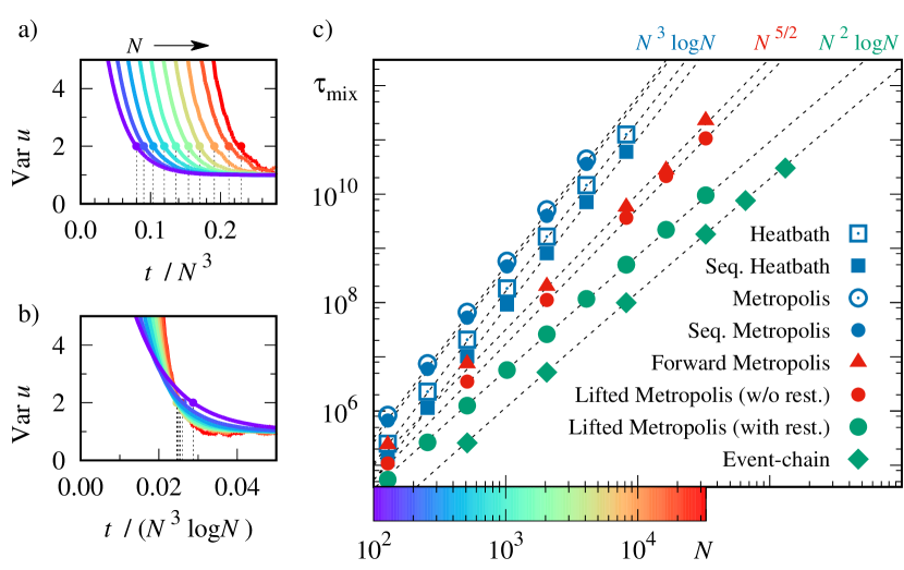
Figure 1: Mixing of local 1D Markov chains. a) Relaxation of $\operatorname{Var}u_{i}$ from the compact initial state under heatbath dynamics ($x$ axis rescaled by $N^{3}$, $y$ axis by equilibrium value). b) Rescaling of $x$ axis with an additional logarithm illustrates $\mathcal{O}(N^{3}\log N)$ time scale. c) Mixing times for the Markov chains discussed in this work. The step $\varepsilon$ is uniformly sampled from $(0;2.5\ell_{\text{free}})$. For the event-chain algorithm, $\tau_{\text{mix}}$ is measured in lifting moves.

In 1D, the thermodynamics and the static correlation functions of finite hard-sphere systems can be computed exactly Tonks (1936); Krauth (2006). Newtonian dynamics is pathological for equal sphere masses, because colliding spheres simply exchange their velocities without mixing them. Stochastic dynamics, however, may converge to equilibrium. For example, reversible heatbath dynamics mixes (that is, converges towards equilibrium from an arbitrary starting configuration) in at most $\sim N^{3}\log N$ individual steps for $N$ spheres Randall and Winkler (2005).

In the present work, we study irreversible local Markov chains for 1D hard-sphere systems that violate the detailed-balance condition yet still converge towards equilibrium. We show by numerical simulation that these irreversible Markov chains typically mix faster than reversible ones, and that they fall into two universality classes (see the Supplemental Material 1 Kapfer and Krauth (2017a) for background on balance conditions and the Supplemental Material 2 for details on mixing and correlation times). The first one mixes in $\mathcal{O}(N^{5/2})$ steps, and is related to the totally asymmetric simple exclusion process (TASEP, see Gwa and Spohn (1992); Chou et al. (2011); Baik and Liu (2016)). The other mixes in $\mathcal{O}(N^{2}\log N)$ and comprises the event-chain algorithm (ECMC) Bernard et al. (2009) and a modified lifted TASEP that we propose in this work. We refer to it as the lifted TASEP class. The framework for our approach to irreversible Markov chains is provided by the lifting concept Chen et al. (1999); Diaconis et al. (2000) together with a factorized Metropolis acceptance rule Michel et al. (2014), which considerably extend the range of applications for irreversible Markov chains (see Ref. Kapfer and Krauth (2017b) for a review). Some evidence for reduced mixing time scales has already been obtained Nishikawa et al. (2015).

In order for a reversible or irreversible Markov chain to converge to the thermodynamic equilibrium given by $\pi$, the total probability flow $\mathcal{F}_{a}$ into a configuration $a$ must satisfy the global balance condition:

$$\mathcal{F}_{a}\equiv\sum_{b}\pi(b)T(b\to a)=\pi(a),$$ (1)

where $T(b\to a)$ is the algorithmic transition probability from $b$ to $a$. In the following, we distinguish between “accepted” flow $\mathcal{A}(b\to a)=\pi(b)T(b\to a)$ from configurations $b\neq a$ to $a$ and “rejected” flow $\mathcal{R}=\pi(a)T(a\to a)$ which results from an attempted move from $a$ that was not accepted. The global balance condition enforces stationarity of $\pi$ under multiplication with the transfer matrix $T$ (see the Supplemental Material 1 for definitions). The special condition realized in reversible Markov chains is the detailed balance $\pi(b)T(b\to a)=\pi(a)T(a\to b)$ which, in terms of the probability flows is simply $\mathcal{A}(a\to b)=\mathcal{A}(b\to a)$, and which implies Eq. 1.

For concreteness, we restrict ourselves to $N$ hard spheres of diameter $d$ on a circle of length $L$, so that the free space is $L_{\text{free}}=L-Nd$, and the mean gap between spheres $\ell_{\text{free}}=L_{\text{free}}/N$. All valid configurations $a$ have the same statistical weight $\pi(a)=1$. They consist in ordered particle positions $a=(\dots x_{i-1},x_{i},x_{i+1},\dots)$ with gap variables $\delta_{i}=x_{i}-x_{i-1}-d\geq 0$ and appropriate periodic boundary conditions. The partition function $Z\sim(L_{\text{free}})^{N}$ is analytic for all densities in the thermodynamic limit, and no phase transition takes place Tonks (1936); Krauth (2006). The model is isomorphic to $N$ point particles on a circle of length $L_{\text{free}}$ with the same gap variables and an interaction $V(\delta_{i}<0)=\infty$ and $V(\delta_{i}\geq 0)=0$ implementing both the non-overlap and the ordering constraint. Because of this mapping onto a gas of free particles with mean gap $\ell_{\text{free}}$, and because the step size distribution of our Markov chains scale with $\ell_{\text{free}}$, their dynamics and in particular their mixing times do not depend on density (see the Supplemental Material 3 for details). Nevertheless, the spatial correlation length of the hard-sphere model diverges in the close-packing limit.

We first consider the reversible heatbath algorithm, which moves at each time step $t=0,1,\dots$ a random sphere $i$ to a random position between spheres $i-1$ and $i+1$ ($x_{i}$ is uniformly sampled in $(x_{i-1}+d,x_{i+1}-d)$). When studying the mixing dynamics, we ignore trivial uniform rotations of the configuration (which only mix in $\sim N^{4}$ steps Randall and Winkler (2005)). We thus restrict our attention to quantities that can be expressed in terms of the $\delta_{i}$ and focus on the slow, large-scale density fluctuations. The reversible heatbath algorithm is known to mix in at most $\sim N^{3}\log N$ steps. We assume that the slowest time scale is exposed by tracking the distribution $\pi(u_{i})$ of any half-system distance $u_{i}=\delta_{i}+\delta_{i+1}+\dotsc+\delta_{i+N/2}$ from a compact initial configuration at $t=0$, where the variance of $u_{i}$ equals $\operatorname{Var}u_{i}=L_{\text{free}}^{2}/4$, towards equilibrium at $t\sim\tau_{\text{mix}}$, where $\operatorname{Var}u_{i}=L_{\text{free}}^{2}/(4N+4)$ (see the Supplemental Material 2 for details). Our simulations indeed show, in agreement with the rigorous bounds Randall and Winkler (2005), that $\sim N^{3}$ steps are insufficient for mixing (see Fig. 1a), while $\sim N^{3}\log N$ steps suffice (see Fig. 1b). The diverging slope of $\operatorname{Var}u_{i}$ at $\tau_{\text{mix}}$ signals the cutoff phenomenon Aldous and Diaconis (1986). Our method also recovers the correct mixing time for the related discrete symmetric SEP model (see below). For this model, the leading term of $\tau_{\text{mix}}$ is known rigorously Lacoin (2017) and scales as $N^{3}\log N$ (notwithstanding the absence of the logarithm in the spectral gap). Our numerical method thus reliably detects mixing times, including logarithmic corrections and prefactors.

Plots analogous to Fig. 1a,b obtain the mixing time scales for all Markov chains studied in the present work (see Fig. 1c). For the heatbath algorithm, a simple scaling argument for the discrete lowest-$k$ Fourier mode $\overline{U}=(u_{1}+u_{2}+\dots+u_{N/2})/N^{3/2}$ yields the $\mathcal{O}(N^{3})$ behavior in equilibrium: In the limit $N\to\infty$, the standard deviation of $\pi(\overline{U})$ is $\mathcal{O}(1)$, and one heatbath step changes $\overline{U}$ by $\mathcal{O}(1/N^{3/2})$. A random walk in $t$ yields:

$$\quad\frac{1}{N^{3/2}}\sqrt{t}\sim 1\implies\tau_{\text{mix}}\gtrsim N^{3}.$$ (2)

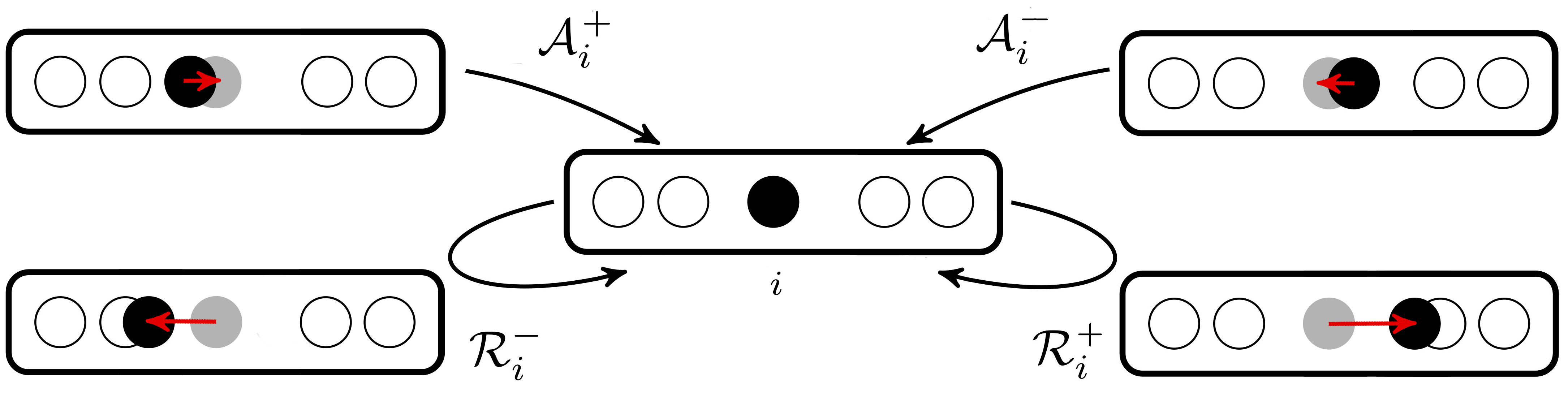
Figure 2: Metropolis flow into configuration $a$ by moves of sphere $i$. For given $\varepsilon$, $\left[\mathcal{A}_{i}^{\pm}(\varepsilon),\mathcal{R}_{i}^{\mp}(\varepsilon)\right]\in\left\{[1,0],[0,1]\right\}$ as a move by $\varepsilon$ is either accepted or rejected. Flows here are integrated over the step distribution $p(\varepsilon)$. The relation $\left[\mathcal{A}_{i}^{+}(\varepsilon),\mathcal{R}_{i-1}^{+}(\varepsilon)\right]\in\left\{[1,0],[0,1]\right\}$ justifies the forward Metropolis algorithm.

The reversible Metropolis algorithm mixes on the same $\mathcal{O}(N^{3}\log N)$ scale as the reversible heatbath algorithm (see Fig. 1c). At each step, it considers a move from $a$ towards a configuration $\tilde{a}$ with $\tilde{x}_{i}=x_{i}+\sigma\varepsilon$, where $\sigma=\pm 1$ samples the forward or backward direction and $\varepsilon>0$ samples the step from some distribution $p(\varepsilon)$ (we use a uniform distribution on the interval $[0;2.5\ell_{\text{free}}]$). If $\tilde{a}$ is invalid because of an overlap or an inversion of $x_{i}$ with $x_{i-1}$ or $x_{i+1}$, the move $a\to a$ results. The reversible Metropolis algorithm satisfies detailed balance between $a$ and any $\tilde{a}$ simply because the moves $\tilde{a}\to a$ and $a\to\tilde{a}$ are equally likely.

The probability flow $\mathcal{F}_{a}$ into $a$ has four components for each sphere $i$ (see Fig. 2), namely accepted forward flow $\mathcal{A}_{i}^{+}=\int\!\mathrm{d}\varepsilon\,p(\varepsilon)\mathcal{A}_{i}^{+}(\varepsilon)$, corresponding to $\sigma=+1$ and analogously accepted backward flow $\mathcal{A}_{i}^{-}$ for $\sigma=-1$. Rejected forward and backward flows $\mathcal{R}_{i}^{+}$ and $\mathcal{R}_{i}^{-}$ from $a$ towards invalid configurations $\tilde{a}$ also contribute to the flow into $a$. For given $\varepsilon$, these flows,

$$\mathcal{A}_{i}^{+}(\varepsilon) =\Theta(\delta_{i}-\varepsilon) \mathcal{R}_{i}^{+}(\varepsilon) =\Theta(\varepsilon-\delta_{i+1})$$ (3)

$$\mathcal{A}_{i}^{-}(\varepsilon) =\Theta(\delta_{i+1}-\varepsilon)\quad \mathcal{R}_{i}^{-}(\varepsilon) =\Theta(\varepsilon-\delta_{i}),$$

(with $\Theta$ the Heaviside step function) are either unity or zero. Moreover, they add up to unity in pairs: $\mathcal{A}_{i}^{+}(\varepsilon)+\mathcal{R}_{i}^{-}(\varepsilon)=1$, $\mathcal{A}_{i}^{-}(\varepsilon)+\mathcal{R}_{i}^{+}(\varepsilon)=1$, because each move is accepted (or rejected) under the same condition as its return move. It follows that for any distribution of $\varepsilon$, the sum of the four flows equals $2$.

Global balance requires the total flow $\mathcal{F}_{a}$ into a valid hard-sphere configuration $a$ to equal $\pi(a)=1$. For the reversible Metropolis algorithm there are $2N$ equal choices of the $N$ spheres and two directions $\sigma=\pm 1$, so that

$$\mathcal{F}_{a}^{\text{rev}}=\frac{1}{2N}\sum_{i}\underbrace{\bigl{(}\mathcal{A}_{i}^{+}+\mathcal{R}_{i}^{+}+\mathcal{A}_{i}^{-}+\mathcal{R}_{i}^{-}\bigr{)}}_{\text{$=2$, see Eq.~{}\ref{e:MetroFlows}}}=1.$$

Global balance is thus established, although it was already implied by the detailed-balance condition.

Global balance is also satisfied for the sequential Metropolis algorithm, the historically first irreversible Markov chain Metropolis et al. (1953), which updates spheres sequentially, say, in ascending order in $i$. At a given time, only a fixed sphere $i$ is updated, and the flow into a configuration $a$ during this move arises from the two choices $\sigma=\pm 1$ for this update of $i$, which each can be either accepted or rejected:

$$\mathcal{F}_{a}^{\text{seq}}=\frac{1}{2}\left(\mathcal{A}_{i}^{+}+\mathcal{R}_{i}^{+}+\mathcal{A}_{i}^{-}+\mathcal{R}_{i}^{-}\right)=1.$$ (4)

Irreducibility and aperiodicity can also be proven for generic distributions $p(\varepsilon)$. With $p(\varepsilon)$ uniform in the interval $[0,2.5\ell_{\text{free}}]$, the sequential Metropolis algorithm mixes $\sim 1.2$ times faster than the reversible Metropolis algorithm, but with the same $\mathcal{O}(N^{3}\log N)$ scaling.

The relation $\mathcal{A}_{i}^{+}(\varepsilon)+\mathcal{R}_{i}^{-}(\varepsilon)=1$ from Eq. 3 can be expressed as $\mathcal{A}_{i}^{+}(\varepsilon)+\mathcal{R}_{i-1}^{+}(\varepsilon)=1$. This motivates the forward Metropolis algorithm, which attempts at each time step a forward move ($\sigma\equiv+1$) sampled from the probability distribution $p(\varepsilon)$, for a randomly sampled sphere $i$. There are now $N$ equal choices for the moves, and the incoming flow into a configuration $a$ is given by

$$\mathcal{F}_{a}^{\text{forw}}=\frac{1}{N}\sum_{i}\underbrace{\left(\mathcal{A}^{+}_{i}+\mathcal{R}^{+}_{i-1}\right)}_{=1}=1,$$ (5)

which again establishes global balance. In contrast, the sequential forward Metropolis algorithm violates global balance. In this algorithm, at a given time step, a fixed sphere $i$ is updated, and the flow $\mathcal{F}_{a}^{\text{seq-forw}}$ into a configuration $a$, at this time step, arises for a given value $\varepsilon$ from a single possible move. The total flow is $\mathcal{F}_{a}^{\text{seq-forw}}=\mathcal{A}^{+}_{i}+\mathcal{R}_{i}^{+}\neq 1$, so that the sequential forward algorithm is not correct.

Remarkably, we find that the forward Metropolis algorithm mixes on a time scale $\mathcal{O}(N^{5/2})$ (see Fig. 1c). The same $N^{5/2}$ time scale also governs the relaxation of the totally asymmetric simple exclusion process (TASEP), a lattice transport model which converges to equilibrium under periodic boundary conditions Baik and Liu (2016). An individual TASEP step attempts to move a randomly-sampled sphere one site to the right (Fig. 3a). Indeed, the TASEP agrees with the forward Metropolis algorithm restricted to integer $x_{i}$ and $L$ and steps $\varepsilon\equiv 1$. By tracking the lattice equivalent of $\operatorname{Var}u_{i}$, we recover the $\mathcal{O}(N^{5/2})$ mixing for the TASEPBaik and Liu (2016), while the symmetric SEP, itself the lattice version of the reversible Metropolis algorithm, mixes in $\sim N^{3}\log N$ Lacoin (2017).

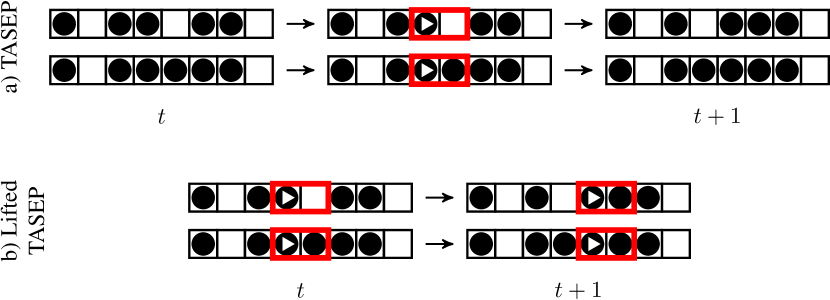
Figure 3: Update rules for discrete models. a) The TASEP advances a random sphere, if possible, and it mixes in $\mathcal{O}(N^{5/2})$. b) The lifted TASEP, without restarts, is deterministic. With restarts, it mixes in $\mathcal{O}(N^{2}\log N)$.

The relation $\mathcal{A}^{+}_{i}(\varepsilon)+\mathcal{R}^{+}_{i-1}(\varepsilon)=1$, for any individual $i$ (see Eq. 5) provides the motivation for the lifted Metropolis algorithm. Here, moves are attempted in the forward direction $\sigma\equiv+1$ but the active sphere $i$ at time step $t+1$ is determined from the outcome at time step $t$ (see Fig. 3b for the discretized example): As long as sphere $i$ can move, it remains active for the next step. Only when it cannot, a lifting move $i\to i+1$ takes place instead and $i+1$ becomes the active sphere (the physical configuration $a$ does not change during this step). Each configuration is now characterized by the active particle $i$, in addition to $a$. The incoming flow $\mathcal{F}_{(a,i)}^{\text{lift}}$ into a lifted configuration $(a,i)$ is either due to an accepted move of $i$ or a rejected move of $i-1$, so that:

$$\mathcal{F}_{(a,i)}^{\text{lift}}=\mathcal{A}^{+}_{i}+\mathcal{R}^{+}_{i-1}=1.$$ (6)

Global balance again holds. We find that the lifted Metropolis algorithm, run as a Markov chain without restarts (see below) mixes in $\mathcal{O}(N^{5/2})$ steps (see Fig. 1c). It thus belongs to the TASEP universality class.

Balance conditions relate the stationary probability distribution $\pi$ at time step $t$ to the distribution at time step $t+1$, which must agree. For the reversible Metropolis algorithm, as discussed, this condition is satisfied for any sequence of $i$ (see Eq. 4). If run for a finite number of steps, the lifted Metropolis algorithm is correct only if started from a random position $i$. It is advantageous to restart this algorithm after $\lambda\sim N$ time steps by resampling the active sphere $i$. The chain length $\lambda$ could also be random, sampled from an appropriate distribution; see the Supplemental Material 4 for details. We then observe mixing on a time scale $\mathcal{O}(N^{2}\log N)$, much faster than all previous Markov chains (see Fig. 1c). The $\mathcal{O}(N^{2})$ time scale is again brought out by a scaling argument for the discrete Fourier mode $\overline{U}$: One chain (sequence of $\sim N$ moves between restarts) of the lifted Metropolis algorithm can change $\overline{U}$ by $\mathcal{O}(1/N^{1/2})$. This change is of random sign. A random walk in $t/N$ then yields $\tau_{\text{mix}}\gtrsim N^{2}$. Simulations indeed show that restarts every $\lambda\sim N$ time steps yield fastest mixing (see Fig. 4a) and outpace restarts with other scalings with $N$ (see Fig. 4b, and below).

The lifted Metropolis algorithm also has a discrete counterpart in the lifted TASEP (see Fig. 3b): A single sphere (occupied lattice site) is active and attempts to advance in forward direction. The sphere remains active if its move is accepted. Otherwise, the lifting index advances to the right-hand neighbor site. The lifted TASEP satisfies global balance, but without restarts fails to be irreducible. With restarts every $\mathcal{O}(N)$ steps, the lifted TASEP also mixes on an $\mathcal{O}(N^{2}\log N)$ time scale. The infinitesimal limit of the lifted Metropolis algorithm, $\varepsilon\to 0$, is the event-chain algorithm (ECMC), which also mixes in $\mathcal{O}(N^{2}\log N)$ lifting moves (see Fig. 1c). It thus also belongs to the lifted TASEP universality class.

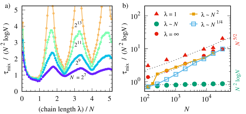
Figure 4: Restarts in the lifted Metropolis algorithm. a) Mixing time as a function of chain length $\lambda\sim N$: The $\mathcal{O}(N^{2}\log N)$ time scale is preserved but mixing is fastest for $\lambda\simeq 0.9N$. b) $\mathcal{O}(N^{5/2})$ mixing for $\lambda\sim N^{1/4}$ (asymptotically equivalent to the (unlifted) forward Metropolis algorithm, $\lambda=1$, red triangles) and for $\lambda\sim N^{2}$ (asymptotically equivalent to lifted Metropolis without any restarts, $\lambda=\infty$, red bullets).

Local 1D Hard-sphere Markov chains		Mixing
Continuous	Discrete	time scale
Heatbath Randall and Winkler (2005), Metropolis	Symm. SEP Lacoin (2017)	$N^{3}\log N$
Forward & Lifted Metrop.	TASEP Baik and Liu (2016)	$N^{5/2}$
Event-chain, Lifted Metrop.	Lifted TASEP	$N^{2}\log N$

Table 1: Mixing time scales for local 1D hard-sphere algorithms on the continuum and on the lattice. The Markov chains on the lowest row all incorporate restarts. See the Supplemental Material 4 for pseudo-code implementations.

The dynamical universality classes for local 1D hard-sphere algorithms are summarized in Table 1. In the lifted TASEP universality class, each sphere only moves $\mathcal{O}(N\log N)$ times to reach equilibrium, almost saturating the lower bound, as $\mathcal{O}(N)$ are required to detach each sphere from the compact initial state.

The irreversible Markov chains presented here are best viewed from their deterministic roots, both on the lattice and in the continuum. Indeed, the lifted TASEP without restarts is a deterministic lattice-gas automaton satisfying global balance, rather than a Markov chain (see Fig. 3b). Irreducibility and aperiodicity call for an element of randomness that can be supplied by restarts. Here, $\lambda\sim N$ (lifted TASEP) and $\lambda\equiv 1$ (TASEP) represent different universality classes. In the continuum, the deterministic root is an algorithm without restarts and invariant step $\varepsilon$, which satisfies global balance. All presented Metropolis-type Markov chains may be obtained from this root by resampling of $i$ or $\varepsilon$. Algorithms belong to different universality classes, depending on the resampling rate: Resampling $\varepsilon$ at every step leads to the lifted Metropolis algorithm without restarts which is in the TASEP class. The additional resampling of $i$ every $\lambda\sim N$ time steps yields the lifted Metropolis algorithm with restarts, which is in the lifted TASEP class (see Fig. 4a, the oscillations suggest that resamplings should ideally correspond to $\sim N/2$ successfully moved spheres and that multiples of $N$ should be avoided). More infrequent restarts ($\lambda\sim N^{2}$) or more frequent ones ($\lambda\sim N^{1/4}$) lead back to the non-lifted TASEP class (see Fig. 4b). Numerical computations of the asymptotic mixing time scales for $\lambda\sim N^{\alpha}$ with $\alpha$ only slightly different from $1$ will require very large system sizes in order to overcome the oscillations at $\alpha=1$.

Injecting randomness with a rate $\sim 1/N$ is thus optimal for mixing. A particular limit of the continuum root algorithm is ECMC without restarts. In 1D, it agrees with Newtonian dynamics with a single sphere of non-zero velocity, and never mixes. Resampling $i$ with rate $\sim 1/N$ (corresponding to an occasional restart of Newtonian dynamics) turns the deterministic dynamics into a very fast local algorithm, the ECMC, which is in the lifted TASEP class, and mixes in $\mathcal{O}(N^{2}\log N)$ lifting moves (see Fig. 1c).

The infinitesimal displacements of ECMC are crucial for its generalization to situations where particles simultaneously interact with several others, such as in more than 1D, or due to long-range forces. This generalization calls for the factorized Metropolis algorithm Michel et al. (2014); Peters and de With (2012); Kapfer and Krauth (2016). The finite-step lifted Metropolis algorithm remains correct for repulsive interactions restricted to nearest neighbors. Indeed, soft repulsive particles with a $1/x^{12}$ potential reproduce the mixing behavior of hard spheres, with $\mathcal{O}(N^{2}\log N)$ mixing for the lifted Metropolis and $\mathcal{O}(N^{5/2})$ mixing for lifted Metropolis without restarts (see the Supplemental Material 5 for details). ECMC has been applied successfully (see Ref. Kapfer and Krauth (2017b) for a review), but prior to the present work, its mixing behavior was not characterized in detail, beyond some partial evidence for faster mixing time scales Nishikawa et al. (2015).

In the future, it will be important to clarify how the different universality classes identified in the present work carry over to higher dimensions and to what degree they depend on the asymmetry of the step distribution. Exact solutions of some of the models in Table 1 may be possible. This would help establish the conceptual framework of lifting and of irreversible Markov chains beyond the single-particle level Diaconis et al. (2000). More generally, the mixing dynamics of hard spheres from an initial compact state may be interpreted as the equilibration process of a physical system in response to a sudden change in its Hamiltonian at time $t=0$. The analysis of the asymmetric evolution of shock fronts may shed further light on the new universality class, as previously for the well-studied TASEP class. An example for a system strongly out of equilibrium, it will be interesting to study how entropy production differs between the three universality classes, and how they may be integrated within the nonequilibrium fluctuation theorems Evans and Searles (2002); Seifert (2012).

I Acknowledgement

SCK thanks the Institut Philippe Meyer for support, and T. Franosch for helpful discussions. We thank the referees for advice on an earlier version of the article.

Supplemental material to “Irreversible local Markov chains with rapid convergence towards equilibrium”

I.1 Supplemental Item 1: Balance conditions, irreducibility, aperiodicity

The mixing of a Markov chain describes how a “worst-case” initial probability distribution $\pi^{t=0}$ converges towards the equilibrium distribution $\pi^{t=\infty}=\pi$. More generally, the time evolution of the distribution $\pi^{t}$ is given by

$$\pi^{t}=T\cdot\pi^{t-1},$$ (S1)

where $T$ is the transfer matrix composed of the algorithmic transition probabilities $T(a\to b)$. This can be expressed as:

$$\pi^{t}(b)=\sum_{a}\pi^{t-1}(a)T(a\to b).$$ (S2)

The steady state, for $t\to\infty$, is defined by $\pi^{t}=\pi^{t-1}=\pi$, and for the hard-sphere system considered in this work it equals $1$ for each valid configuration. For Eq. S2 to be valid, the global balance condition must hold:

$$\pi(b)=\sum_{a}\pi(a)T(a\to b)=\sum_{a}\mathcal{F}_{a\to b}.$$ (S3)

The global-balance condition thus states that the probability flow from all configurations $a$ (including $b$) into $b$ must equal $\pi(b)$. Because of $\sum_{c}T(b\to c)=1$ (if the Markov chain continues, it must go somewhere starting from $b$, maybe even back to $c=b$), it can also be written as

$$\sum_{a}\mathcal{F}_{a\to b}=\pi(b)=\sum_{c}\mathcal{F}_{b\to c},$$ (S4)

that is, the flow into $b$ equals the flow out of $b$. The detailed-balance condition

$$\pi(b)T(b\to a)=\pi(a)T(a\to b)\equiv\mathcal{F}_{b\to a}=\mathcal{F}_{a\to b}\quad\forall a,b$$ (S5)

implies global balance, but it is more restrictive on the algorithmic transition probabilities $T(a\to b)$. It implies that the steady-state flow is reversible and that the net flow $\mathcal{F}_{a\to b}-\mathcal{F}_{b\to a}$ between any $a$ and $b$ vanishes.

For the lifted Metropolis algorithm treated in this work, the configurations are defined by the lifting variables in addition to the “physical” configurations. The global balance condition then requires that the flow into a “lifted” configuration $(a,i)$ equals the weight of $(a,i)$, which is $\pi[(a,i)]=\pi(a)=1$.

Besides the global balance condition, the Markov chain must satisfy two further conditions in order to be sure to converge to the probability distribution $\pi$ in the limit of infinite times. The irreducibility condition requires that for every pair of states $a,b$, there exists a natural number $m$ such that $(T^{m})_{ab}>0$, i. e., if the Markov chain starts at $a$, with $\pi^{0}(a)=1$, there is a finite probability $\pi^{m}(b)$. This condition (in the physics literature often called “ergodicity”) ensures that there is only a single stationary solution of Eq. S3, and that it is reached from an arbitrary initial condition. The event-chain algorithm without restarts violates the irreducibility condition, because after each event, the position $x_{i}$ of sphere $i$ comes to equal $x_{i+1}-d$. For $d=0$, for example, the set of the $N-1$ positions at event times does not change with time. Nevertheless, restarts reinstall the irreducibility. Finally, the Markov chain must satisfy the aperiodicity condition, which means that it should be free of cycles. All Markov chains discussed in this work are aperiodic.

I.2 Supplemental Item 2: Rigorous and operational definitions of mixing time

Rigorously, a Markov chain’s approach to equilibrium is quantified through the total variation distance between the finite-time probability distributions $\pi^{t}$ and the stationary solution $\pi=\pi^{t=\infty}$:

$$||\pi^{t}-\pi||=\frac{1}{2}\sum_{j}|\pi^{t}(j)-\pi(j)|.$$ (S6)

Here, $\pi^{t}=T^{t}\pi^{0}$ depends on the initial distribution $\pi^{0}$ chosen. The total variation distance of Eq. S6 approaches zero as $t\to\infty$, which is equivalent to the statement that the Markov chain defined by $T$ mixes. The mixing time, for a given tolerance $\varepsilon$, is defined as the time at which the total variation distance drops below $\varepsilon$ from a “worst-case” initial state $\pi^{\text{w.c.}}$:

$$\max_{i}||T^{t}\pi^{\text{w.c.}}-\pi||\leq\varepsilon\quad\text{for all $t\geq\tau_{\text{mix}}(\varepsilon)$}.$$ (S7)

The mixing time thus determines the time it takes to obtain a first (single) sample of the equilibrium distribution. The mixing time is usually larger than the correlation time (given by the inverse spectral gap of the transfer matrix), the time it takes to move from one equilibrium configuration to another.

For the Markov chains discussed in this work, we do not compute the mixing time rigorously and rather suppose that the “worst-case” initial distribution is realized when all the spheres $i,i+1,\dots,N,N+1,\dots,N+i-1$, are compactly spaced by the sphere diameter $d$. We then track the approach towards equilibrium through what we suppose to be the slowest variable, namely the half-system distance $u$ between any particle $i$ and particle $i+N/2$ (with periodic boundary conditions applied):

$$u=\underbrace{\delta_{i+N/2}+\dotsc+\delta_{i+1}}_{\text{$N/2$ terms}}.$$ (S8)

Because of periodic boundary conditions, thermal averages of this quantity do not depend on $i$. The probability distribution $\pi(u)$ can be computed exactly (see Krauth (2006)):

$$\pi(u) =\frac{\Gamma(N-1)}{L_{\text{free}}^{N-1}}\frac{(L_{\text{free}}u-u^{2})^{N/2-1}}{(N/2-1)!^{2}}.$$ (S9)

We obtain

$$\langle u\rangle =L_{\text{free}}/2,$$

$$\langle u^{2}\rangle =\frac{L_{\text{free}}^{2}(N+2)}{4(N+1)},$$

$$\operatorname{Var}u =\frac{N^{2}\ell_{\text{free}}^{2}}{4(N+1)}.$$ (S10)

In the compact initial configuration, $\operatorname{Var}u$ takes the value

$$\operatorname{Var}_{\text{compact}}(u)=\langle u^{2}\rangle_{\text{compact}}-\langle u\rangle^{2}_{\text{compact}}=\frac{N^{2}\ell_{\text{free}}^{2}}{4}.$$

In Fig. 1c of the main text, we track the ratio of the empirical variance of the half-system distance and of the exact equilibrium variance given by Eq. S10. We note that this ratio has to go from $\mathcal{O}(N)$ at $t=0$ towards $\sim 1$ at $t\sim\tau_{\text{mix}}$.

I.3 Supplemental Item 3: Density independence of Heatbath and Metropolis algorithms

In higher dimensions, a Monte Carlo algorithm for hard-sphere systems is defined for moves $\mathbf{x}_{i}\to\mathbf{x}_{i}+\boldsymbol{\varepsilon}$ that must satisfy a non-overlap condition which forces the centers of spheres $i$ and $j$ (both of diameter $d$) to remain distant by more than $d$. In one dimension, one may complement this by an ordering constraint $x_{i}<x_{i+1}$ (with appropriate periodic boundary conditions). A move can thus be rejected for two reasons:

1. A physical overlap of two spheres,

2. A violation of the imposed ordering of spheres (an inversion).

These two conditions are respected if a move $x_{i}\to x_{i}+\varepsilon$ (with $\varepsilon$ larger or smaller than $0$) is accepted only if

$$\underbrace{x_{i-1}-x_{i}+d}_{\text{$-\delta_{i}$, ``left'' gap variable}}<\varepsilon<\underbrace{x_{i+1}-x_{i}-d}_{\text{$\delta_{i+1}$, ``right'' gap variable}}.$$ (S11)

It follows that two starting configurations with different values of the $x_{i}$ and $d$ but the same gap variables $\delta_{i}$ perform equivalently under the same Monte Carlo dynamics. Furthermore, two starting configurations and Monte Carlo algorithms with gap variables and distribution $p(\varepsilon)$ scaled by the same factor also realize the same dynamics. It also follows from this simple analysis of the Monte Carlo dynamics that the one-dimensional hard-sphere model cannot have a phase transition (as the sphere diameter $d$ does not modify the dynamics) and that the dynamics, at constant $N$, is independent of the density $Nd/L$ if the distribution of $\varepsilon$ scales with $\ell_{\text{free}}$ (for example, if $\varepsilon$ is a uniform random number in $[0;2.5\ell_{\text{free}}]$, as used in the main text).

I.4 Supplemental Item 4: Pseudo-code implementations of the 1D hard-sphere Metropolis algorithms

In the following pseudo-code implementations of the algorithms discussed in the main text, we suppose real-valued ordered positions $x_{i}<x_{i+1}$. We identify particles $i$ and $i\pm N$, and implicitly apply periodic boundary conditions for the positions, $x_{i}+L\equiv x_{i+N}$.

I.4.1 Reversible Metropolis algorithm

The reversible Metropolis algorithm satisfies detailed balance, as discussed in the main text. The algorithm remains correct for arbitrary interaction potentials if the move from $a$ towards a trial configuration $b$ is accepted with the standard Metropolis acceptance filter $\min[1,\pi(b)/\pi(a)]$ (Metropolis et al. (1953), see Krauth (2006)).

(S12)

I.4.2 Sequential Metropolis algorithm

The sequential Metropolis algorithm performs a sequence of one-particle updates which individually satisfy detailed balance, but the sequence as a whole violates detailed balance. As discussed in the main text, the sequential Metropolis, introduced in Metropolis et al. (1953), is the historically first irreversible Markov chain. The increasing sequence of spheres used in the following pseudo-code implementation can be replaced any other sequence that updates each sphere $i$ with finite frequency. The sequential Metropolis algorithm remains correct for arbitrary interaction potentials if the move from $a$ towards a trial configuration $b$ is accepted with the standard Metropolis acceptance filter $\min[1,\pi(b)/\pi(a)]$ (Metropolis et al. (1953), see Krauth (2006)).

(S13)

I.4.3 Forward Metropolis algorithm

The forward Metropolis algorithm moves spheres only in positive direction ($\sigma=+1$). As discussed in the main text, the uniform random sampling of the sphere index $i$ is essential to insure that this algorithm satisfies the global-balance condition (for example, we prove in the main text that the sequential forward Metropolis algorithm is incorrect.)

(S14)

I.4.4 Lifted Metropolis algorithm (without restarts)

In the lifted Metropolis algorithm without restarts, all spheres move in positive direction $\sigma=+1$. Only the active sphere $i$ can move, and $i$ remains active after a move of $i$ that was accepted. Otherwise, the lifting move $i\to i+1$ ensues. Initially, $i$ must be chosen uniformly among all spheres, although this is only relevant for small running times $t_{\max}$. As illustrated in the following pseudo-code implementation, both the physical move and the lifting move count as one time step. The algorithm is irreducible for a general distribution of steps $p(\varepsilon)$.

(S15)

I.4.5 Lifted Metropolis algorithm (with restarts)

The lifted Metropolis algorithm with restarts is obtained from the previous lifted Metropolis algorithm by resampling the active sphere $i$ (uniformly among all spheres) after $\lambda$ time steps. (The below algorithm continues to satisfy global balance if the same $\varepsilon$ is chosen for the whole chain $c$, rather than to resample it at each time step). $\lambda$ may be a random positive integer, or a constant. For best efficiency, the distribution of chain lengths $p(\lambda)$ should be chosen such that $\langle\lambda\rangle_{p}\sim N$, i. e., a typical chain traverses an extensive part of the system. This ensures that the algorithm is in the lifted TASEP class.

(S16)

I.4.6 Event-chain algorithm

The hard-sphere event-chain Monte Carlo algorithm Bernard et al. (2009) remains valid in arbitrary dimensions. It generalizes to arbitrary interactions using the factorized Metropolis acceptance rule Michel et al. (2014). For simplicity, the following pseudo-code only treats one-dimensional hard spheres, where it presents the continuum limit $\varepsilon\to 0$, $\lambda\to\infty$, $\varepsilon\lambda=\ell$ of the lifted Metropolis with restarts Eq. S16. Restarts are essential for irreducibility of the algorithm. The distribution of chain lengths $\ell$ should be chosen such that $\langle\ell\rangle_{p}\sim L_{\text{free}}$, i. e., a typical chain traverses an extensive part of the system. This ensures that the algorithm is in the lifted TASEP class.

(S17)

I.5 Supplemental Item 5: Lifted forward Metropolis algorithm with soft potentials

The global-balance algorithms discussed in the main text (with finite $\varepsilon$) remain valid under the condition that the interaction is restricted to only nearest neighbors, is monotonous and that it enforces the ordering constraint $x_{i+1}>x_{i}$. Under these conditions, the weight $\pi(a)$ can be written as

$$\pi(a)=\prod_{m=1}^{N}\tilde{\pi}(x_{m+1}-x_{m}),$$ (S18)

where periodic boundary conditions are again assumed, and the function $\tilde{\pi}(\Delta x)$ monotonically increases with $\Delta x$ and is zero for $\Delta x<0$. In addition, the move from a configuration $a$ (with positions $x$) to a configuration $b$ (with positions $x^{\prime}$) is accepted with the factorized Metropolis filter Michel et al. (2014)

$$P_{\text{acc}}(a\to b)=\prod_{m}\min\left[1,\frac{\tilde{\pi}(x^{\prime}_{m+1}-x^{\prime}_{m})}{\tilde{\pi}(x_{m+1}-x_{m})}\right].$$ (S19)

For the considered move $x_{i}\to x_{i}^{\prime}=x_{i}+\varepsilon$ with $\varepsilon>0$, only two terms in Eq. S19 have to be considered (and only one of them contributes), namely

$$\min\left[1,\frac{\tilde{\pi}(x_{i}+\varepsilon-x_{i-1})}{\tilde{\pi}(x_{i}-x_{i-1})}\right]=1\quad\text{and}\quad\min\left[1,\frac{\tilde{\pi}(x_{i+1}-x_{i}-\varepsilon)}{\tilde{\pi}(x_{i+1}-x_{i})}\right]=\frac{\tilde{\pi}(x_{i+1}-x_{i}-\varepsilon)}{\tilde{\pi}(x_{i+1}-x_{i})}\leq 1.$$ (S20)

Note that because of the monotonicity of the weights, $\tilde{\pi}(x_{i}+\varepsilon-x_{i-1})\geq\tilde{\pi}(x_{i}-x_{i-1})$, etc. It follows that the move $x_{i}\to x_{i}+\varepsilon$ is accepted with probability

$$P_{\text{acc}}(x_{i}\to x_{i}+\varepsilon)=\frac{\tilde{\pi}(x_{i+1}-x_{i}-\varepsilon)}{\tilde{\pi}(x_{i+1}-x_{i})}.$$ (S21)

As in the main text, we have to show that the flow $\mathcal{F}_{(a,i)}^{\text{lift}}$ into a lifted configuration $(a,i)$ (either due to an accepted move of sphere $i$ or to a rejected move of sphere $i-1$) satisfies

$$\mathcal{F}_{(a,i)}^{\text{lift}}=\mathcal{A}^{+}_{i}+\mathcal{R}^{+}_{i-1}=\pi(a),$$ (S22)

where $\mathcal{A}^{+}_{i}=\int\mathrm{d}\varepsilon p(\varepsilon)\mathcal{A}^{+}_{i}(\varepsilon)$, and analogous for $\mathcal{R}^{+}_{i-1}$. But this follows because, for any fixed $\varepsilon>0$, the accepted flow corresponds to a move of sphere $i$ from $x_{i}-\varepsilon$ to $x_{i}$:

$$\mathcal{A}^{+}_{i}(\varepsilon) =\pi(\dots,x_{i-1},x_{i}-\varepsilon,x_{i+1},\dots)P_{\text{acc}}(x_{i}-\varepsilon\to x_{i})$$

$$=\left[\dots\tilde{\pi}(x_{i}-x_{i-1}-\varepsilon)\tilde{\pi}(x_{i+1}-x_{i}+\varepsilon)\tilde{\pi}(x_{i+2}-x_{i+1})\dots\right]\frac{\tilde{\pi}(x_{i+1}-x_{i})}{\tilde{\pi}(x_{i+1}-x_{i}+\varepsilon)}$$

and because the rejected flow corresponds to a (rejected) move of sphere $i-1$ from $x_{i-1}$ to $x_{i-1}+\varepsilon$:

$$\mathcal{R}^{+}_{i-1}(\varepsilon) =\pi(\dots,x_{i-1},x_{i},x_{i+1},\dots)\left[1-P_{\text{acc}}(x_{i-1}\to x_{i-1}+\varepsilon)\right]$$

$$=\left[\dots\tilde{\pi}(x_{i}-x_{i-1})\tilde{\pi}(x_{i+1}-x_{i})\tilde{\pi}(x_{i+2}-x_{i+1})\dots\right]\left[1-\frac{\tilde{\pi}(x_{i}-x_{i-1}-\varepsilon)}{\tilde{\pi}(x_{i}-x_{i-1})}\right]$$

Thus Eq. S22 holds irrespective of the distribution $p(\varepsilon)$.

We have implemented soft-potential version of the Metropolis algorithms discussed in the main text for a $1/x^{12}$ potential, and confirmed that without restarts, it belongs to the TASEP universality class, and with restarts every $\lambda\sim N$ steps, to the lifted TASEP class, see Fig. S1 panels b) and c). In the same system, the reversible Metropolis algorithm mixes as $\mathcal{O}(N^{3}\log N)$, just as in hard spheres. The severe conditions on the applicability of the lifted Metropolis finite-$\varepsilon$ algorithm disappear in the limit $\varepsilon\to 0$, that is, for the generalized event-chain algorithm Michel et al. (2014), see Fig. S1a).

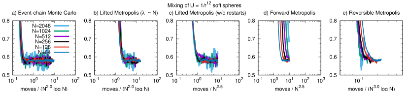
Figure S1: Mixing of Metropolis-type Markov chains with a $1/x^{12}$ soft potential. We plot the quantity $\operatorname{Var}u$ on the vertical axis, and rescale the number of moves on the horizontal axis to extract the scaling of the mixing time $\tau_{\text{mix}}$ with $N$. a) and b) With restarts every $\lambda\sim N$ moves, the lifted Metropolis and event-chain algorithms are in the lifted TASEP class. c) The lifted Metropolis without restarts is in the TASEP class, $\tau_{\text{mix}}=\mathcal{O}(N^{5/2})$. d) The forward Metropolis algorithm for soft spheres mixes slower than $\mathcal{O}(N^{5/2})$, apparently requiring logarithmic corrections. e) The reversible Metropolis algorithm with a factorized filter mixes in $\mathcal{O}(N^{3}\log N)$. For this system, $\tilde{\pi}(x)=\exp(-\Gamma x^{-12})$ for $x>0$ and $\tilde{\pi}(x)=0$ otherwise.

References

- Kirkwood and Monroe (1941) J. G. Kirkwood and E. Monroe, J. Chem. Phys. 9, 514 (1941).
- Hoover and Ree (1968) W. G. Hoover and F. H. Ree, J. Chem. Phys. 49, 3609 (1968).
- Alder and Wainwright (1962) B. J. Alder and T. E. Wainwright, Phys. Rev. 127, 359 (1962).
- Bernard and Krauth (2011) E. P. Bernard and W. Krauth, Phys. Rev. Lett. 107, 155704 (2011).
- Asakura and Oosawa (1954) S. Asakura and F. Oosawa, J. Chem. Phys. 22, 1255 (1954).
- Krauth (2006) W. Krauth, Statistical Mechanics: Algorithms and Computations (Oxford University Press, 2006).
- Halperin and Nelson (1978) B. I. Halperin and D. R. Nelson, Phys. Rev. Lett. 41, 121 (1978).
- Young (1979) A. P. Young, Phys. Rev. B 19, 1855 (1979).
- Alder and Wainwright (1957) B. J. Alder and T. E. Wainwright, J. Chem. Phys. 27, 1208 (1957).
- Alder and Wainwright (1970) B. J. Alder and T. E. Wainwright, Phys. Rev. A 1, 18 (1970).
- Parisi and Zamponi (2010) G. Parisi and F. Zamponi, Rev. Mod. Phys. 82, 789 (2010).
- Torquato and Stillinger (2010) S. Torquato and F. H. Stillinger, Rev. Mod. Phys. 82, 2633 (2010).
- Metropolis et al. (1953) N. Metropolis, A. W. Rosenbluth, M. N. Rosenbluth, A. H. Teller, and E. Teller, J. Chem. Phys. 21, 1087 (1953).
- Kannan et al. (2003) R. Kannan, M. W. Mahoney, and R. Montenegro, in Proc. 14th annual ISAAC, Lecture Notes in Computer Science (Springer, Berlin, Heidelberg, 2003) pp. 663–675.
- Tonks (1936) L. Tonks, Phys. Rev. 50, 955 (1936).
- Randall and Winkler (2005) D. Randall and P. Winkler, “Mixing points on a circle,” in Approximation, Randomization and Combinatorial Optimization, Lecture Notes in Computer Science, Vol. 3624, edited by C. Chekuri et al. (Springer, Berlin, Heidelberg, 2005).
- Kapfer and Krauth (2017a) S. C. Kapfer and W. Krauth, (2017a), supplemental Material XXXX.
- Gwa and Spohn (1992) L.-H. Gwa and H. Spohn, Phys. Rev. Lett. 68, 725 (1992).
- Chou et al. (2011) T. Chou, K. Mallick, and R. K. P. Zia, Rep. Prog. Phys. 74, 116601 (2011).
- Baik and Liu (2016) J. Baik and Z. Liu, J. Stat. Phys. 165, 1051 (2016).
- Bernard et al. (2009) E. P. Bernard, W. Krauth, and D. B. Wilson, Phys. Rev. E 80, 056704 (2009).
- Chen et al. (1999) F. Chen, L. Lovász, and I. Pak, Proc. 17th Ann. ACM Symp. Theory of Computing , 275 (1999).
- Diaconis et al. (2000) P. Diaconis, S. Holmes, and R. M. Neal, Ann. Appl. Probab. 10, 726 (2000).
- Michel et al. (2014) M. Michel, S. C. Kapfer, and W. Krauth, J. Chem. Phys. 140, 054116 (2014).
- Kapfer and Krauth (2017b) S. C. Kapfer and W. Krauth, (2017b), to appear in EPJB.
- Nishikawa et al. (2015) Y. Nishikawa, M. Michel, W. Krauth, and K. Hukushima, Phys. Rev. E 92, 063306 (2015).
- Aldous and Diaconis (1986) D. Aldous and P. Diaconis, Am. Math. Monthly 93, 333 (1986).
- Lacoin (2017) H. Lacoin, Ann I H Poincaré-Pr 53, 1402 (2017).
- Peters and de With (2012) E. A. J. F. Peters and G. de With, Phys. Rev. E 85, 026703 (2012).
- Kapfer and Krauth (2016) S. C. Kapfer and W. Krauth, Phys. Rev. E 94, 031302 (2016).
- Evans and Searles (2002) D. J. Evans and D. J. Searles, Adv. Phys. 51, 1529 (2002).
- Seifert (2012) U. Seifert, Rep. Prog. Phys. 75, 126001 (2012).