TARGET-QUALITY IMAGE COMPRESSION WITH RECURRENT, CONVOLUTIONAL NEURAL NETWORKS

Abstract

We introduce a stop-code tolerant (SCT) approach to training recurrent convolutional neural networks for lossy image compression. Our methods introduce a multi-pass training method to combine the training goals of high-quality reconstructions in areas around stop-code masking as well as in highly-detailed areas. These methods lead to lower true bitrates for a given recursion count, both pre- and post-entropy coding, even using unstructured LZ77 code compression. The pre-LZ77 gains are achieved by trimming stop codes. The post-LZ77 gains are due to the highly unequal distributions of 0/1 codes from the SCT architectures. With these code compressions, the SCT architecture maintains or exceeds the image quality at all compression rates compared to JPEG and to RNN auto-encoders across the Kodak dataset. In addition, the SCT coding results in lower variance in image quality across the extent of the image, a characteristic that has been shown to be important in human ratings of image quality.

Index Terms—  Image Compression, Neural Networks, Adaptive Encoding

1 INTRODUCTION

Earlier work has shown the power of convolutional neural networks in compressing images, both under a single-bitrate target [1] and under multiple-bitrate targets [2, 3]. Both approaches are better than JPEG compression, as long as entropy coding is used on their output symbols [1, 2]. To date, both types of neural networks have suffered from the constraint that their output codes have a fixed symbol dimension (“depth”) over the full extent of the image. In [1], the number of symbols is completely defined by the depth of the bottleneck layer. Similarly, [2] allows for different quality levels, by changing the number of iterations, but the number of iterations is fixed across the full image, giving an equal number of symbols to each area of the image. We seek to send fewer symbols in simpler sections of the image, allowing us to send additional symbols on more difficult-to-compress sections. This allows neural-network based systems to see gains similar to whose from run-length encoding in JPEG DCT coefficient transmission.

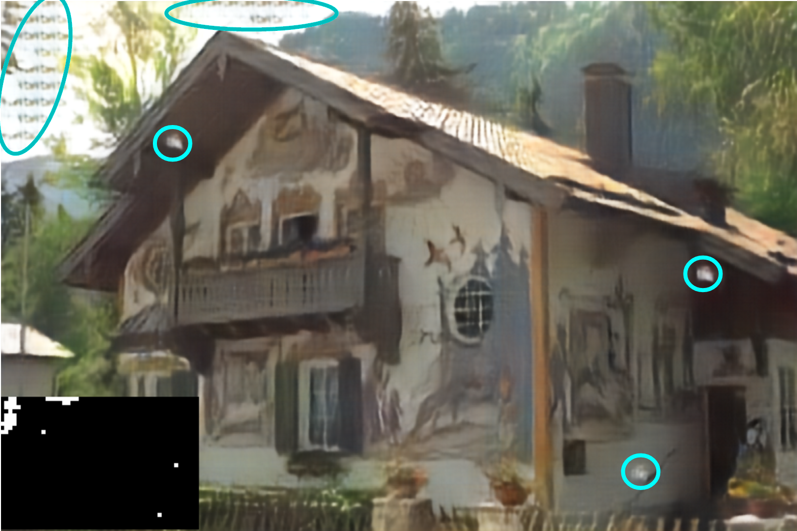
(a) 0.121 bpp non-SCT

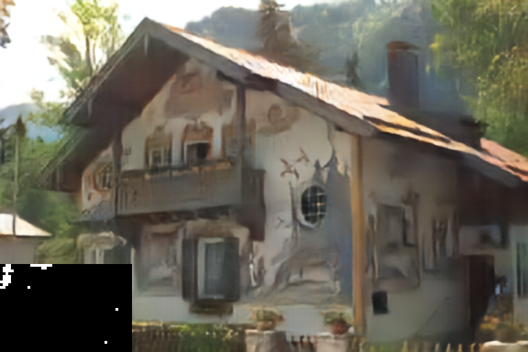
(b) 0.115 bpp SCT

Fig. 1: Examples of recursive compression at 0.125 bpp (nominal), with the stop-code mask in the lower-left corner. (a) Output from LSTM, additive, adaptive-gain network trained as described in [2]; after gzip coding this is 0.121 bpp. Code-trimming-induced artifacts are circled in cyan. (b) Same architecture but trained as described in Section 3; after gzip coding this is 0.115 bpp. Using this modified training, we avoid artifacts from code trimming.

The difficulty in stop codes and code trimming in recursive neural networks (RNNs) is their convolutional nature results in wide spatial dependence on symbols that are omitted (due to earlier stop codes). Simple training approaches for stop-code tolerant (SCT) RNNs tend to produce blocking artifacts and blurry reconstructions. The blocking artifacts in the areas around the stop-code-induced gaps (Figure 1) are due to the RNN’s convolutions relying on neighbor codes too heavily and then failing when those codes are omitted. Blurry reconstructions are due to the learning process attempting to accommodate code trimming even in complicated image patches.

This paper introduces a two-pass approach to training RNN’s for high-quality image reconstruction with stop codes and code trimming: On each iteration, the first pass trains the decoder network with examples that include stop-code masking and the second trains for accurate reconstructions. By introducing the first pass, the full training process (both early and late) includes the SCT requirement, allowing the network to converge to symbol assignments that both satisfy the stop code structure and provide representational power.

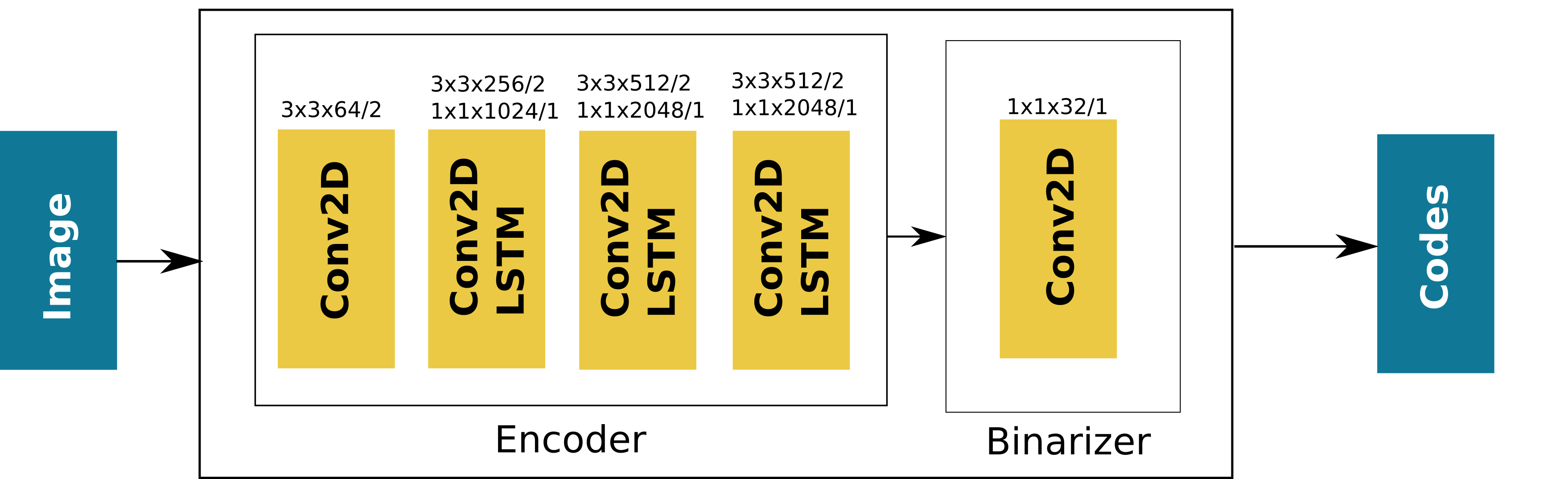
(a) Encoder and binarizer used by both non-SCT and SCT networks.

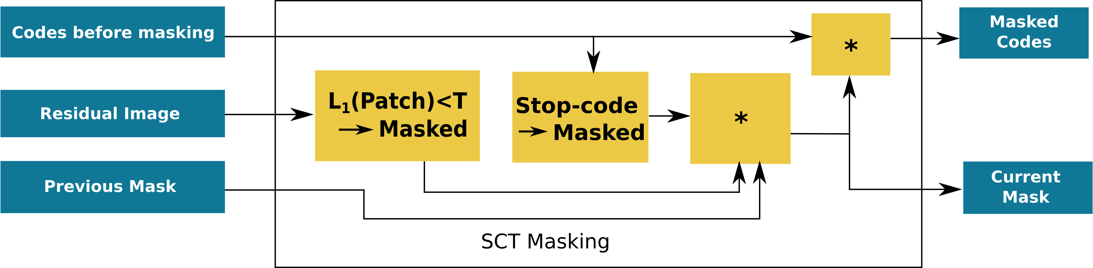
(b) SCT-network masking logic, to enforce stop-code behavior.

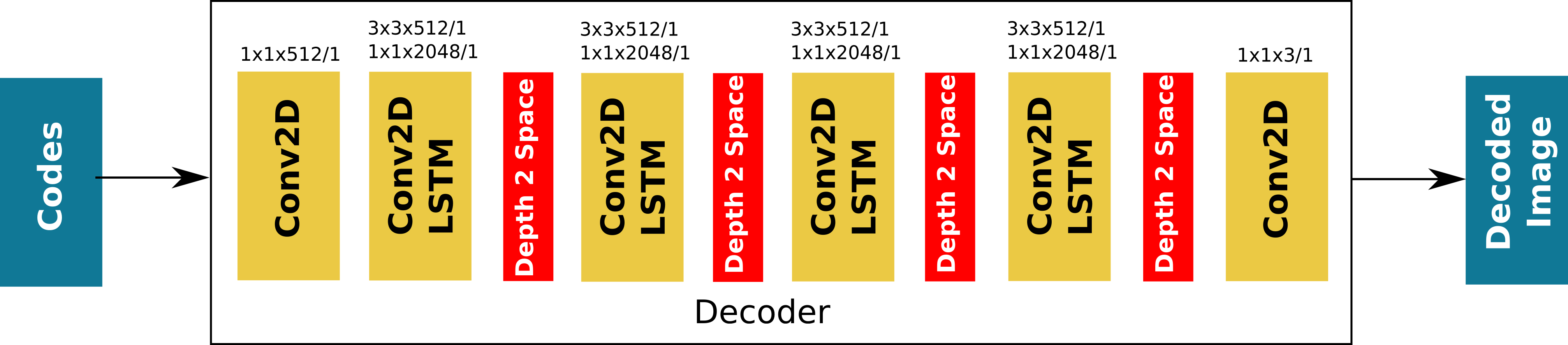
(c) Decoder used by both non-SCT and SCT networks.

Fig. 2: Block diagram for both non-SCT (by omitting b) and SCT (by including b). Parameters for the convolution layers are listed as HxWxD/S, for kernels that are HxW with D channels and a stride of S. Convolutional LSTMs list input convolutions above hidden-state convolutions. The masking logic ensures that once a stop code is emitted (whether accidentally or deliberately), all subsequent iterations feed a stop code at that tile to the decoder.

2 PREVIOUS WORK

Our research is based on the confluence of two long-running areas of research: image compression [4, 5, 6] and neural-network-based ‘auto-encoders’ [7, 8, 9]. Recurrent autoencoders have been successfully applied to the problem of variable-rate image compression [10, 2] while feedforward neural networks have been equally successful at fixed-rate encoding [1]. This previous work in neural-network-based compression implicitly allocates the same number of symbols to each local ‘tile’ of the image: there was no equivalent to code trimming as seen in JPEG [4] via run-length encoding.

In this paper, we focus on training fully convolutional, recurrent neural networks to handle stop codes. A parallel effort in this area [11] looks at solving the same data-adaptive coding problem by moving to a block-based approach, like JPEG and WebP. In contrast, this paper’s work remains in the fully-convolutional framework and establishes a predictible stop code, both to signal to the decoder that a tile is entering code trimming and to allow the decoder to fill in all subsequent unsent (stop) codes for that tile.

3 METHOD

For our SCT approach, we start by using the architecture of one of the best variable-rate-encoding architectures from [2]: LSTM (Residual Scaling). In the encoder network (Figure 2-a), LSTM (Residual Scaling) interleaves LSTM units with four layers of spatial downsampling, giving the binarizer a $\frac{H}{16}\times\frac{W}{16}$ representation of the $H\times W$ image. In the decoder network (Figure 2-c), a full $H\times W$ reconstruction is created from the $\frac{H}{16}\times\frac{W}{16}$ codes using ‘depth-to-space’ shuffling [12]. In this paper, we refer to this baseline as the “non-SCT” network. Figure 2 shows the architectures of our non-SCT model (by excluding Figure 2-b) and our SCT model (by including Figure 2-b). As mentioned above, spatial downsampling in the encoder results in the binarizer outputting one stack of bi-level (-1/1) codes for each $16\times 16$ spatial ‘tile’ from the input image but the image-tile–to–code-stack mapping is not the same as the blocks used in JPEG or BPG [6]: the convolutional support of the encoder network results in spatial dependences far beyond this downsampling-induced $16\times 16$ association.

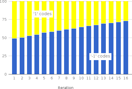
(a) non-SCT -1/1 frequencies

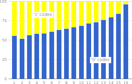
(b) SCT 0/1 frequencies

Fig. 3: The SCT architecture produces more biased code distributions than does the non-SCT, making LZ77 more effective, especially on later iterations.

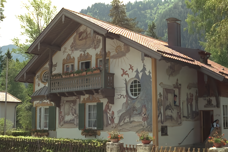
(a) 0.791 bpp SCT reconstruction

(b) 0.745 bpp non-SCT

(c) quality comparison

Fig. 4: Image reconstructions near 0.75 bpp. (a) Reconstruction from SCT architecture at 0.791 bpp ($7^{th}$ iteration which gives the closes true bpp to target). (b) Reconstruction from non-SCT architecture at 0.745 bpp ($6^{th}$ iteration). (c) Quality differences between SCT and non-SCT reconstructions. SCT gives lower $L_{1}$ error on 65.0% of the image (white); non-SCT gives lower error on 11.5% of the image (black); and they are effectively equal ($\pm\frac{1}{2}$ out of 256) on 23.5% of the image (gray).

In [2], the actual bit rates were measured by running the binarizer codes through a custom-trained entropy coder. For the sake of time and clarity, we instead use Lempel–Ziv coding (LZ77) [13] on the flat file that contains the codes. Note that LZ77 compression is less effective than what is possible with a custom entropy coder, since LZ77 does not exploit the underlying spatial and depth structure of the codes.

We make minimal architecture modifications to go from the non-SCT network to our SCT network. We modify the binarizer  [2] to use 0/1, instead of -1/1, to avoid boundary artifacts at the edges of images. We also add a masking process after the binarizer layer, but before “code transmission” (Figure 2-b), to enforce our stop-code behaviors. The mask is computed at the end of each iteration, setting to all ‘0’ (masked) those tiles: (a) where the reconstruction quality for the tile exceeds our target quality level; (b) where the output of the encoder network for this iteration is (accidently) the all-zero stop code; or (c) where the codes were masked off on an earlier iteration. This masking logic allows us to treat an all-zero code as a stop code and to avoid sending any of that tile’s subsequent iterations: the code itself communicates the stop condition. Since the decoder is able to compute the mask for each iteration without any additional information, we explicitly provide the mask as input into the decoder.

The SCT behavior of our trained networks derives from the training loss that we use. Our training loss includes the ‘reconstruction loss’ used in [2]. If this is the only term that is used (as it was in [2]), image regions near masked bits result in highly visible blocking artifacts (Figure 1). In addition to the reconstruction-error term, we add a penalty for non-zero bits in our codes: this helps bias our code distributions towards zero bits (Figure 3), making entropy compression more effective.

The training approach that we found to work best for creating SCT networks is to create a combined loss function from two interleaved reconstruction passes: one pass to train for accurate reconstructions and one pass to train for stop-code tolerance. Without the SCT pass, the networks would not see masked codes and code trimming until very late in the training process. By that point in training, they are less able to adjust to the masked codes without the types of artifacts shown in Figure 1-a: they already have effectively made symbol assignments at the bottleneck/binarizer that can not conform to an all-zero stop code.

To allow this two-pass training, for each mini-batch in the training, just before the $k^{th}$ iteration, we record $S^{k-1}$ and $C^{k-1}$, the ‘state’ and ‘cell’ vectors for all of the decoder’s LSTM units and $E_{\max}^{k-1}$ and $E_{\min}^{k-1}$, the maximum and minimum reconstruction errors on that mini batch. We then run the $k^{th}$, iteration twice, by restoring the LSTM memory to $S^{k-1}$ and $C^{k-1}$ between the two passes at the $k^{th}$ iteration.

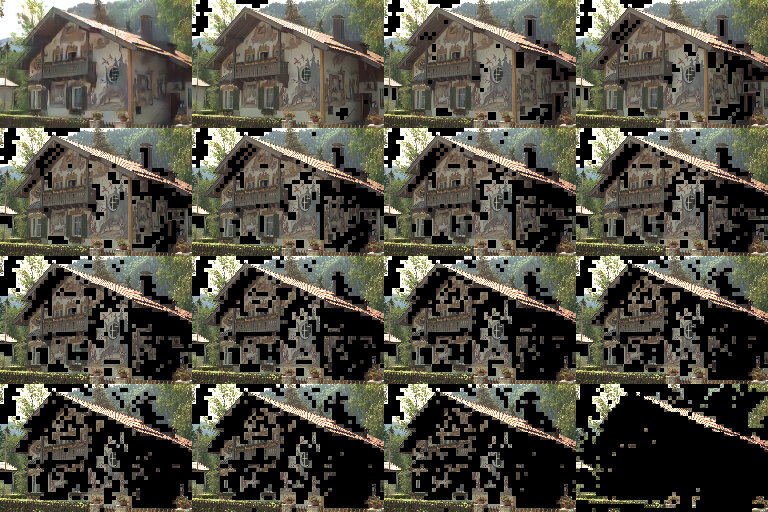
Fig. 5: Visualization of coding progress in SCT method. Each image represents a new iteration. Trimmed codes are represented by masked portions of the image. Areas where the $L_{1}$ error remains above threshold continue to transmit codes, up to our iteration limit.

First, we introduce a SCT-training pass through each iteration in order to allow the neural network to learn on examples with masked codes. To present the network with reasonable examples of masked codes, we set an artificially high masking threshold, creating a ‘fake’ mask that will always have some masked-off areas. In the masked-off areas, we reset all of the bits that will be seen by the decoder to zero, just as they would have been if the mask were generated naturally, with the regular masking threshold. We set the artificially high masking threshold to $(k/K*(E_{\max}^{k-1}-E_{\min}^{k-1})+E_{\min}^{k-1})$ where $K$ is the maximum number of iterations over which we are training. We add the $L_{1}$ reconstruction error of the output generated by these forced-mask iterations to the reconstruction-error loss from the “natural-mask” reconstruction (the second pass). Note that the forced-mask reconstruction builds on the natural-mask reconstruction for all the iterations prior to the current iteration.

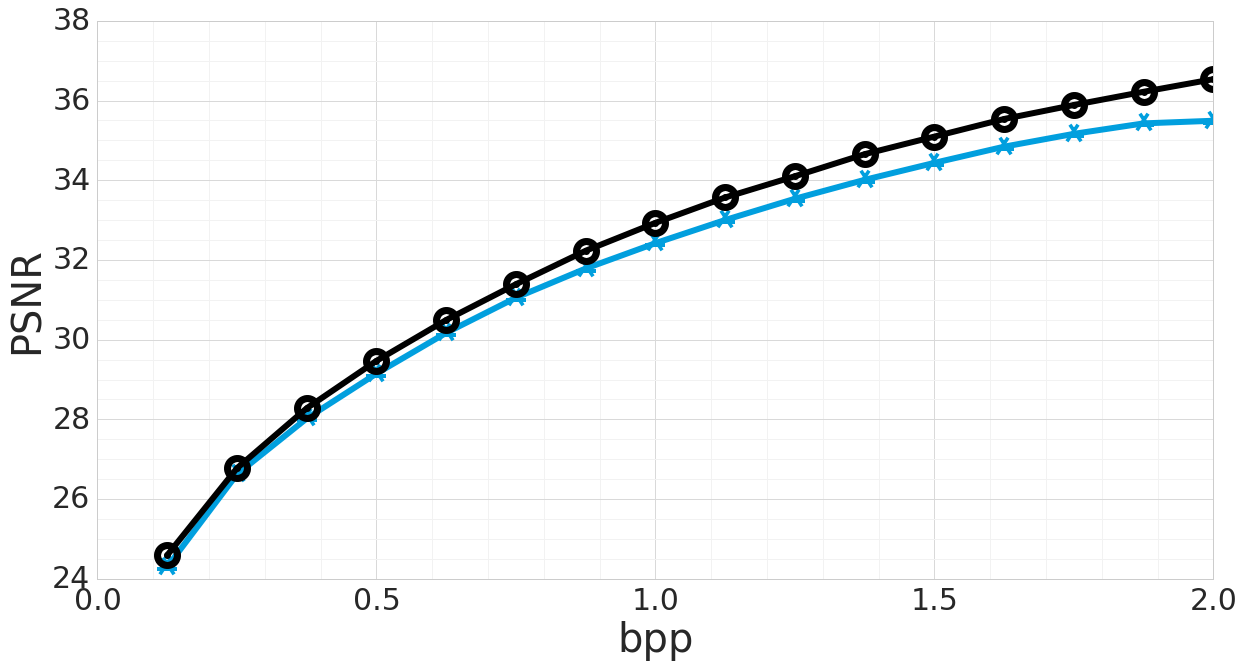
(a) PSNR vs nominal bitrate

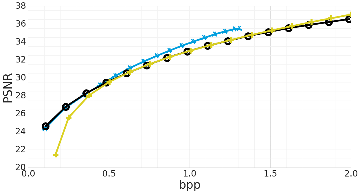
(b) PSNR vs true bitrate

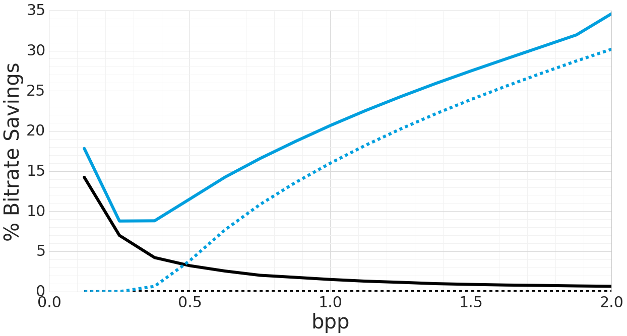
(c) Bitrate savings from LZ77 and code trimming

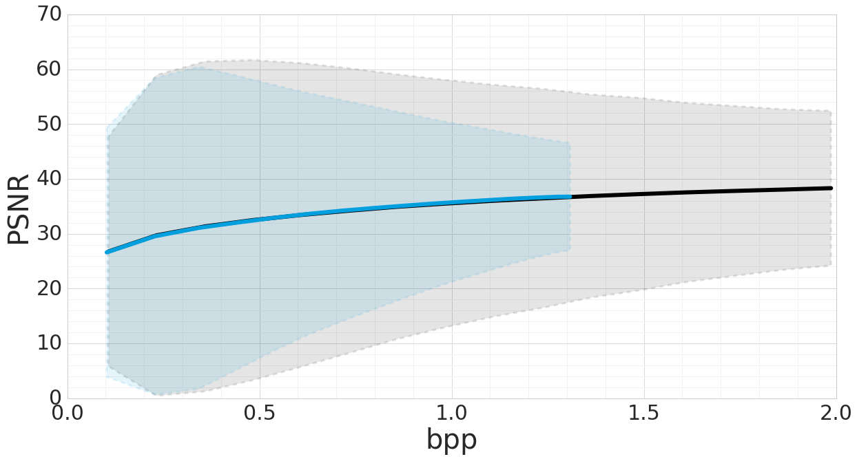
(d) Within-image quality variance

Fig. 6: This figure shows results on the Kodak dataset, with the black lines for non-SCT coding [2] and blue lines for our SCT method: (a) PSNR Rate-distortion (RD) curve, using the nominal bitrate: neither stop-code trimming nor LZ77 is done, so the RD curve for the non-SCT coding is higher. (b) PSNR RD curve using LZ77 compression and stop-code trimming: black line for [2] after LZ77; blue line for EST coding with stop-code trimming and LZ77; yellow line for JPEG420. (c) Percent bitrate savings for SCT coding (blue) and [2] (black) over the nominal bitrate: hashed lines show bitrate savings from stop-code trimming; solid lines show savings including LZ77. (d) Reduction in within-image variance in reconstruction quality using SCT coding: gray shading shows within-reconstruction-image variance with [2]; blue shading shows same with EST coding.

We then run a second pass through the iteration, after restoring $S^{k-1}$ and $C^{k-1}$, so that the previous (forced-masking) pass through the $k^{th}$ iteration does not impact our results. In this second pass, we use the masks generated ‘naturally’ by the expanding the previous iteration’s (natural) mask according to the stop codes present in the current iteration’s (natural) binary codes. This reconstruction is used to form the main reconstruction error (and its corresponding loss), just as it was in [2]. It is the $S^{k}$, $C^{k}$, $E_{\max}^{k}$ and $E_{\min}^{k}$ values from this ‘natural’ decoding that are recorded before the next iteration is run.

4 RESULTS

Figures 1 and 4 provide examples of the difference between non-SCT and SCT reconstructions, for 0.12 bpp and for 0.75 bpp true bit rate (that is, the bitrate after LZ77/stop-trimming). At 0.12 bpp, the non-SCT reconstruction is sharper than the SCT reconstruction (see the vertical edges in Figure 1-b) but the quality of the SCT reconstruction is more uniform than the non-SCT reconstruction (Figure 1-a). At 0.75 bpp, the SCT reconstruction is nearly uniformly better than the non-SCT reconstruction (see Figure 4-c) and is a more uniform quality across the reconstruction.

Figure 5 shows how the SCT reconstruction progresses across iterations. Almost a third of the codes are trimmed before the $10^{th}$ iteration. More than 80% of the codes are trimmed before the $16^{th}$ iteration on this image.

Figure 6-a and 6-b show the rate-distortion (RD) curves for SCT and non-SCT [2] coding, using the nominal bitrate and the bitrate with LZ77/stop-trimming, respectively. If the nominal bitrate is used, SCT coding does worse than non-SCT coding. This is expected since the SCT architecture is required to balance reconstruction quality with robustness to code trimming (to provide SCT) and reduction in bit-level entropy (to improve LZ77). Figure 6-b shows that the SCT more than makes up for this nominal loss, once stop-code trimming and LZ77 are used to be provide a more accurate RD curve.

In Figure 6-c, we show the amount of gain due to LZ77 on both non-SCT and SCT codes. We also show the gains due to trimming stop codes (that is, all zeros) after the transmission of the first instance of that in a given tile. With the non-SCT codes, we see less than 1% additional bitrate compression using LZ77 at the higher bit rates. In contrast, we see a 35% bitrate reduction in SCT codes over the nominal bitrates: about 30% due to stop-code trimming and the last 5% due to LZ77.

To compare the uniformity of the image quality within a reconstruction, we took a reconstruction from the non-SCT architecture at 0.745 bpp (after LZ77) and a reconstruction from the SCT architecture that was closest to that same bitrate (after stop-code trimming and LZ77) and compared the $L_{1}$ error in each $32\times 32$ section of the image. Figure 4-c shows black where the SCT reconstruction is worse than the non-SCT reconstruction and white were it is better. The image areas where SCT reconstruction is worse than non-SCT are those areas where the reconstructions are already quite good, so stop coding has been used (compare Figure 4-c to the first and second line of Figure 5). The $L_{1}$ tile-error mean and, more importantly, standard deviations are both 11% lower for the EST reconstruction than for the non-EST reconstruction: for near 0.75 bpp on this image, it is 4.7 vs 5.3 for the mean and 4.3 vs 4.8 for the standard deviation.

5 CONCLUSIONS

This work has introduced a training method to allow neural-network based compression systems to adaptively vary the number of symbols transmitted for different parts of the compressed image, based on the local underlying content. Our method allows the networks to remain fully convolutional, thereby avoiding the blocking artifacts that often accompany block-based approaches at low bit rates. We have shown promising results with this approach on a recursive auto-encoder structure which was originally reported in [2].

There are many interesting directions to extend the current work. The most immediate would be to train and apply neural-network-based entropy coding [2], to exploit the known spatial structure. Longer term, one interesting area is to consider changing the stop-code threshold on a per-iteration basis, to encourage even more uniform quality distributions. Another research direction is to take this same SCT idea and apply it to non-recurrent auto-encoders. This would require assigning “priority” to different sections of the auto-encoder’s bottleneck, as well as determining the best stop-code structure.

References

- [1] J. Ballé, V. Laparra, and E. Simoncelli, “End-to-end optimized image compression,” CoRR, vol. abs/1611.01704, 2016.
- [2] G. Toderici, D. Vincent, N. Johnston, S.J. Hwang, D. Minnen, J. Shor, and M. Covell, “Full resolution image compression with recurrent neural networks,” CoRR, vol. abs/1608.05148, 2016.
- [3] K. Gregor, F. Besse, D. Jimenez Rezende, I. Danihelka, and D. Wierstra, “Towards Conceptual Compression,” ArXiv e-prints, 2016.
- [4] W. Pennebaker and J. Mitchell, JPEG: Still Image Compression Standard, Kluwer Academic Publishers, 1992.
- [5] Google, “WebP: Compression techniques (http://developers.google.com/speed/webp/docs/compression),” Accessed: 2017-01-30.
- [6] F. Bellard, “BPG image format (http://bellard.org/bpg/),” Accessed: 2017-01-30.
- [7] G. E. Hinton and R. R. Salakhutdinov, “Reducing the dimensionality of data with neural networks,” Science, vol. 313, no. 5786, pp. 504–507, 2006.
- [8] A. Krizhevsky and G. E. Hinton, “Using very deep autoencoders for content-based image retrieval,” in European Symposium on Artificial Neural Networks, 2011.
- [9] P. Vincent, H. Larochelle, Y. Bengio, and P.-A. Manzagol, “Extracting and composing robust features with denoising autoencoders,” Journal of Machine Learning Research, 2012.
- [10] G. Toderici, S. O’Malley, S.J. Hwang, D. Vincent, D. Minnen, S. Baluja, M. Covell, and R. Sukthankar, “Variable rate image compression with recurrent neural networks,” ICLR 2016, 2016.
- [11] D. Minnen, G. Toderici, M. Covell, T. Chinen, N. Johnston, J. Shor, S.J. Hwang, D. Vincent, and S. Singh, “Spatially adaptive image compression using a tiled deep network,” submission to ICIP 2017.
- [12] M. Abadi, A. Agarwal, P. Barham, E. Brevdo, Z. Chen, C. Citro, G. Corrado, A. Davis, J. Dean, M. Devin, S. Ghemawat, I. Goodfellow, A. Harp, G. Irving, M. Isard, Y. Jia, R. Jozefowicz, L. Kaiser, M. Kudlur, J. Levenberg, D. Mané, R. Monga, S. Moore, D. Murray, C. Olah, M. Schuster, J. Shlens, B. Steiner, I. Sutskever, K. Talwar, P. Tucker, V. Vanhoucke, V. Vasudevan, F. Viégas, O. Vinyals, P. Warden, M. Wattenberg, M. Wicke, Y. Yu, and X. Zheng, “TensorFlow: Large-scale machine learning on heterogeneous systems (http://tensorflow.org),” 2015, Software available from tensorflow.org.
- [13] J.-L. Gailly, “GNU Gzip: General file (de)compression (http://www.gnu.org/software/gzip/manual/gzip.html),” Accessed: 2017-01-30.