Kernel clustering: density biases and solutions

Abstract

Kernel methods are popular in clustering due to their generality and discriminating power. However, we show that many kernel clustering criteria have density biases theoretically explaining some practically significant artifacts empirically observed in the past. For example, we provide conditions and formally prove the density mode isolation bias in kernel K-means for a common class of kernels. We call it Breiman’s bias due to its similarity to the histogram mode isolation previously discovered by Breiman in decision tree learning with Gini impurity. We also extend our analysis to other popular kernel clustering methods, e.g. average/normalized cut or dominant sets, where density biases can take different forms. For example, splitting isolated points by cut-based criteria is essentially the sparsest subset bias, which is the opposite of the density mode bias. Our findings suggest that a principled solution for density biases in kernel clustering should directly address data inhomogeneity. We show that density equalization can be implicitly achieved using either locally adaptive weights or locally adaptive kernels. Moreover, density equalization makes many popular kernel clustering objectives equivalent. Our synthetic and real data experiments illustrate density biases and proposed solutions. We anticipate that theoretical understanding of kernel clustering limitations and their principled solutions will be important for a broad spectrum of data analysis applications across the disciplines.

1 Introduction

uniform density data
	(a) K-means	(b) kernel K-means
non-uniform data
	(c) kernel K-means	(d) kernel clustering
	(Breiman’s bias, mode isolation)	(adaptive weights or kernels)

Figure 1: Kernel K-means with Gaussian kernel (1) gives desirable nonlinear separation for uniform density clusters (a,b). But, for non-uniform clusters in (c) it either isolates a small dense “clump” for smaller $\sigma$ due to Breiman’s bias (Section 2) or gives results like (a) for larger $\sigma$. No fixed $\sigma$ yields solution (d) given by locally adaptive kernels or weights eliminating the bias (Sections 4 & 3).

In machine learning, kernel clustering is a well established data analysis technique [1, 2, 3, 4, 5, 6, 7, 8, 9, 10] that can identify non-linearly separable structures, see Figure 1(a-b). Section 1.1 reviews the kernel K-means and related clustering objectives, some of which have theoretically explained biases, see Section 1.2. In particular, Section 1.2.2 describes the discrete Gini clustering criterion standard in decision tree learning where Breiman [11] proved a bias to histogram mode isolation.

Empirically, it is well known that kernel K-means or average association (see Section 1.1.1) has a bias to so-called “tight” clusters for small bandwidths [3]. Figure 1(c) demonstrates this bias on a non-uniform modification of a typical toy example for kernel K-means with common Gaussian kernel

$$k(x,y)\propto\exp\left(-\frac{\|x-y\|^{2}}{2\sigma^{2}}\right).$$ (1)

This paper shows in Section 2 that under certain conditions kernel K-means approximates the continuous generalization of the Gini criterion where we formally prove a mode isolation bias similar to the discrete case analyzed by Breiman. Thus, we refer to the “tight” clusters in kernel K-means as Breiman’s bias.

We propose a density equalization principle directly addressing the cause of Breiman’s bias. First, Section 3 discusses modification of the density with adaptive point weights. Then, Section 4 shows that a general class of locally adaptive geodesic kernels [10] implicitly transforms data and modifies its density. We derive “density laws” relating adaptive weights and kernels to density transformations. They allow to implement density equalization resolving Breiman’s bias, see Figure 1(d). One popular heuristic [12] approximates a special case of our Riemannian kernels.

Besides mode isolation, kernel clustering may have the opposite density bias, e.g. sparse subsets in Normalized Cut [3], see Figure 9(a). Section 5 presents “normalization” as implicit density inversion establishing a formal relation between sparse subsets and Breiman’s bias. Equalization addresses any density biases. Interestingly, density equalization makes many standard kernel clustering criteria conceptually equivalent, see Section 6.

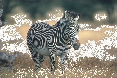
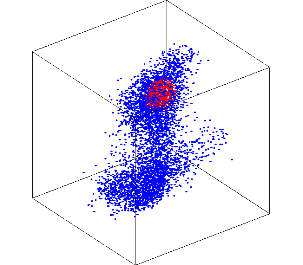
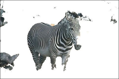
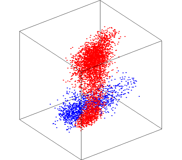
(a) Breiman’s bias	(b) good clustering

Figure 2: Example of Breiman’s bias on real data. Feature vectors are 3-dimensional LAB colours corresponding to image pixels. Clustering results are shown in two ways. First, red and blue show different clusters inside LAB space. Second, pixels with colours in the “background” (red) cluster are removed from the original image. (a) shows the result for kernel K-means with a fixed-width Gaussian kernel isolating a small dense group of pixels from the rest. (b) shows the result for an adaptive kernel, see Section 4.

1.1 Kernel K-means

A popular data clustering technique, kernel K-means [1] is a generalization of the basic K-means method. Assuming $\Omega$ denotes a finite set of points and $f_{p}\in\mathcal{R}^{N}$ is a feature (vector) for point $p$, the basic K-means minimizes the sum of squared errors within clusters, that is, distances from points $f_{p}$ in each cluster $S_{k}\subset\Omega$ to the cluster means $m_{k}$

$$\left(\parbox{38.74988pt}{\centering\bf\small k-means criterion\@add@centering}\right)\quad\quad\quad\quad\quad\quad\sum_{k}\sum_{p\in S^{k}}\|f_{p}-m_{k}\|^{2}.\quad\quad\quad\quad$$ (2)

Instead of clustering data points $\{f_{p}\;|\;p\in\Omega\}\subset\mathcal{R}^{N}$ in their original space, kernel K-means uses mapping $\phi\;\;:\;\;\mathcal{R}^{N}\rightarrow\mathcal{H}$ embedding input data $f_{p}\in\mathcal{R}^{N}$ as points $\phi_{p}\equiv\phi(f_{p})$ in a higher-dimensional Hilbert space $\mathcal{H}$. Kernel K-means minimizes the sum of squared errors in the embedding space corresponding to the following (mixed) objective function

$$F(S,m)\;\;=\;\;\sum_{k}\sum_{p\in S^{k}}\|\phi_{p}-m_{k}\|^{2}$$ (3)

where $S=(S^{1},S^{2},\dots,S^{K})$ is a partitioning (clustering) of $\Omega$ into $K$ clusters, $m=(m_{1},m_{2},\dots m_{K})$ is a set of parameters for the clusters, and $\|.\|$ denotes the Hilbertian norm. Kernel K-means finds clusters separated by hyperplanes in $\mathcal{H}$. In general, these hyperplanes correspond to non-linear surfaces in the original input space $\mathcal{R}^{N}$. In contrast to (3), standard K-means objective (2) is able to identify only linearly separable clusters in $\mathcal{R}^{N}$.

Optimizing $F$ with respect to the parameters yields closed-form solutions corresponding to the cluster means in the embedding space:

$$\hat{m}_{k}=\frac{\sum_{q\in S^{k}}\phi_{q}}{|S^{k}|}$$ (4)

where $|.|$ denotes the cardinality (number of points) in a cluster. Plugging optimal means (4) into objective (3) yields a high-order function, which depends solely on the partition variable $S$:

$$F(S)\;\;=\;\;\sum_{k}\sum_{p\in S^{k}}\left\|\phi_{p}-\frac{\sum_{q\in S^{k}}\phi_{q}}{|S^{k}|}\right\|^{2}.$$ (5)

Expanding the Euclidean distances in (5), one can obtain an equivalent pairwise clustering criterion expressed solely in terms of inner products $\langle\phi(f_{p}),\phi(f_{q})\rangle$ in the embedding space $\mathcal{H}$:

$$F(S)\;\;\mbox{$\;\overset{c}{=}\;$}\;\;-\sum_{k}\frac{\sum_{pq\in S^{k}}\langle\phi(f_{p}),\phi(f_{q})\rangle}{|S^{k}|}$$ (6)

where $\;\overset{c}{=}\;$ means equality up to an additive constant. The inner product is often replaced with kernel $k$, a symmetric function:

$$k(x,y):=\langle\phi(x),\phi(y)\rangle.$$ (7)

Then, kernel K-means objective (5) can be presented as

$$\left(\parbox{38.74988pt}{\centering\bf\small kernel \\ k-means criterion\@add@centering}\right)\quad\quad\quad F(S)\;\;\mbox{$\;\overset{c}{=}\;$}\;\;-\sum_{k}\frac{\sum_{pq\in S^{k}}k(f_{p},f_{q})}{|S^{k}|}.\quad$$ (8)

Formulation (8) enables optimization in high-dimensional space $\mathcal{H}$ that only uses kernel computation and does not require computing the embedding $\phi(x)$. Given a kernel function, one can use the kernel K-means without knowing the corresponding embedding. However, not any symmetric function corresponds to the inner product in some space. Mercer’s theorem [2] states that any positive semidefinite (p.s.d.) kernel function $k(x,y)$ can be expressed as an inner product in a higher-dimensional space. While p.s.d. is a common assumption for kernels, pairwise clustering objective (8) is often extended beyond p.s.d. affinities. There are many other extension of kernel K-means criterion (8). Despite the connection to density modes made in our paper, kernel clustering has only a weak relation to mean-shift [13], e.g. see [14].

1.1.1 Related graph clustering criteria

Positive semidefinite kernel $k(f_{p},f_{q})$ in (8) can be replaced by an arbitrary pairwise similarity or affinity matrix $A=[A_{pq}]$. This yields the average association criterion, which is known in the context of graph clustering [3, 15, 7]:

$$-\sum_{k}\frac{\sum_{pq\in S^{k}}A_{pq}}{|S^{k}|}.$$ (9)

The standard kernel K-means algorithm [7, 9] is not guaranteed to decrease (9) for improper (non p.s.d.) kernel $k:=A$. However, [15] showed that dropping p.s.d. assumption is not essential: for arbitrary association $A$ there is a p.s.d. kernel $k$ such that objective (8) is equivalent to (9) up to a constant.

In [3] authors experimentally observed that the average association (9) or kernel K-means (8) objectives have a bias to separate small dense group of data points from the rest, e.g. see Figure 2.

Besides average association, there are other pairwise graph clustering criteria related to kernel K-means. Normalized cut is a common objective in the context of spectral clustering [3, 16]. It optimizes the following objective

$$-\sum_{k}\frac{\sum_{pq\in S^{k}}A_{pq}}{\sum_{p\in S^{k}}d_{p}}.$$ (10)

where $d_{p}=\sum_{q\in\Omega}A_{pq}$. Note that for $d_{p}=1$ equation (10) reduces to (9). It is known that Normalized cut objective is equivalent to a weighted version of kernel K-means criterion [17, 7].

1.1.2 Probabilistic interpretation via kernel densities

Besides kernel clustering, kernels are also commonly used for probability density estimation. This section relates these two independent problems. Standard multivariate kernel density estimate or Parzen density estimate for the distribution of data points within cluster $S^{k}$ can be expressed as follows [18]:

$$\mbox{${\cal P}_{\Sigma}$}(x|S^{k})\;\;:=\;\;\frac{\sum_{q\in S^{k}}k(x,f_{q})}{|S^{k}|},$$ (11)

with kernel $k$ having the form:

$$k(x,y)\;\;=\;\;|\Sigma|^{-\frac{1}{2}}\;\mbox{$\psi$}\left(\Sigma^{-\frac{1}{2}}(x-y)\right)$$ (12)

where $\psi$ is a symmetric multivariate density and $\Sigma$ is a symmetric positive definite bandwidth matrix controlling the density estimator’s smoothness. One standard example is the Gaussian (normal) kernel (1) corresponding to

$$\mbox{$\psi$}(t)\;\propto\;\exp\left(-\frac{\|t\|^{2}}{2\;}\right),$$ (13)

which is commonly used both in kernel density estimation [18] and kernel clustering [6, 3].

The choice of bandwidth $\Sigma$ is crucial for accurate density estimation, while the choice of $\psi$ plays only a minor role [19]. There are numerous works regarding kernel selection for accurate density estimation using either fixed [20, 19, 21] or variable bandwidth [22]. For example, Scott’s rule of thumb is

$$\sqrt{\Sigma_{ii}}=\frac{r_{i}}{\sqrt[N+4]{n}},\quad\quad\Sigma_{ij}=0\text{ for }i\neq j$$ (14)

where $n$ is the number of points, and $r_{i}^{2}$ is the variance of the $i$-th feature that could be interpreted as the range or scale of the data. Scott’s rule gives optimal mean integrated squared error for normal data distribution, but in practice it works well in more general settings. In all cases the optimal bandwidth for sufficiently large datasets is a small fraction of the data range [23, 18]. For shortness, we use adjective $r$-small to describe bandwidths providing accurate density estimation.

If kernel $k$ has form (12) up to a positive multiplicative constant then kernel K-means objective (8) can be expressed in terms of kernel densities (11) for points in each cluster [6]:

$$F(S)\;\mbox{$\;\overset{c}{=}\;$}\;-\sum_{k}\sum_{p\in S^{k}}\mbox{${\cal P}_{\Sigma}$}(f_{p}|S^{k}).$$ (15)

1.2 Other clustering criteria and their known biases

One of the goals of this paper is a theoretical explanation for the bias of kernel K-means with small bandwidths toward tight dense clusters, which we call Breiman’s bias, see Figs 1-2. This bias was observed in the past only empirically. As discussed in Section 4.1, large bandwidth reduces kernel K-means to basic K-means where bias to equal cardinality clusters is known [24]. This section reviews other standard clustering objectives, entropy and Gini criteria, that have biases already well-understood theoretically. In Section 2 we establish a connection between Gini clustering and kernel K-means in case of $r$-small kernels. This connection allows theoretical analysis of Breiman’s bias in kernel K-means.

1.2.1 Probabilistic K-means and entropy criterion

Besides non-parametric kernel K-means clustering there are well-known parametric extensions of basic K-means (2) based on probability models. Probabilistic K-means [24] or model based clustering [25] use some given likelihood functions $P(f_{p}|\theta_{k})$ instead of distances $\|f_{p}-\theta_{k}\|^{2}$ in (2) as in clustering objective

$$-\sum_{k}\sum_{p\in S^{k}}\log P(f_{p}|\theta_{k}).$$ (16)

Note that objective (16) reduces to basic K-means (2) for Gaussian probability model $P(.|\theta_{k})$ with mean $\theta_{k}$ and a fixed scalar covariance matrix.

In probabilistic K-means (16) models can differ from Gaussians depending on a priori assumptions about the data in each cluster, e.g. gamma, Gibbs, or other distributions can be used. For more complex data, each cluster can be described by highly-descriptive parametric models such as Gaussian mixtures (GMM). Instead of kernel density estimates in kernel K-means (15), probabilistic K-means (16) uses parametric distribution models. Another difference is the absence of the $\log$ in (15) compared to (16).

The analysis in [24] shows that in case of highly descriptive model $P$, e.g. GMM or histograms, (16) can be approximated by the standard entropy criterion for clustering:

$$\left(\parbox{38.74988pt}{\centering\bf\small entropy \\ criterion\@add@centering}\right)\quad\quad\quad\quad\quad\sum_{k}|S^{k}|\cdot H(S^{k})\quad\quad\quad\quad\quad\quad\quad$$ (17)

where $H(S^{k})$ is the entropy of the distribution of the data in $S^{k}$:

$$H(S^{k})\;\;:=\;\;-\int P(x|\theta_{k})\log P(x|\theta_{k})\,\mathrm{d}x.$$

The discrete version of the entropy criterion is widely used for learning binary decision trees in classification [11, 18, 26]. It is known that the entropy criterion above is biased toward equal size clusters [11, 24, 27].

1.2.2 Discrete Gini impurity and criterion

Both Gini and entropy clustering criteria are widely used in the context of decision trees [18, 26]. These criteria are used to decide the best split at a given node of a binary classification tree [28]. The Gini criterion can be written for clustering $\{S^{k}\}$ as

$$\left(\parbox{55.97205pt}{\centering\bf\small discrete \\ Gini criterion\@add@centering}\right)\quad\quad\quad\quad\quad\sum_{k}|S^{k}|\cdot G(S^{k})\quad\quad\quad\quad\quad$$ (18)

where $G(S^{k})$ is the Gini impurity for the points in $S^{k}$. Assuming discrete feature space $\cal L$ instead of $\mathcal{R}^{N}$, the Gini impurity is

$$G(S^{k})\;:=\;1-\sum_{l\in\cal L}\mbox{${\cal P}$}(l\,|S^{k})^{2}$$ (19)

where $\mbox{${\cal P}$}(\cdot\,|S^{k})$ is the empirical probability (histogram) of discrete-valued features $f_{p}\in\cal L$ in cluster $S^{k}$.

Similarly to the entropy, Gini impurity $G(S^{k})$ can be viewed as a measure of sparsity or “peakedness” of the distribution for points in $S^{k}$. Note that (18) has a form similar to the entropy criterion in (17), except that entropy $H$ is replaced by the Gini impurity. Breiman [11] analyzed the theoretical properties of the discrete Gini criterion (18) when $\mbox{${\cal P}$}(\cdot\,|S^{k})$ are discrete histograms. He proved

Theorem 1 (Breiman).

For $K=2$ the minimum of the Gini criterion (18) for discrete Gini impurity (19) is achieved by assigning all data points with the highest-probability feature value in $\mathcal{L}$ to one cluster and the remaining data points to the other cluster, as in example for $\mathcal{L}=\{1,\dots,14\}$ on the left. ∎

2 Breiman’s bias (numerical features)

In this section we show that the kernel K-means objective reduces to a novel continuous Gini criterion under some general conditions on the kernel function, see Section 2.1. We formally prove in Section 2.2 that the optimum of the continuous Gini criterion isolates the data density mode. That is, we show that the discussed earlier biases observed in the context of clustering [3] and decision tree learning [11] are the same phenomena. Section 2.3 establishes connection to maximum cliques [29] and dominant sets [8].

For further analysis we reformulate the problem of clustering a discrete set of points $\{f_{p}\,|\,p\in\Omega\}\subset\mathcal{R}^{N}$, see Section 1.1, as a continuous domain clustering problem. Let $P$ be a probability measure over domain $\mathcal{R}^{N}$ and $\rho$ be the corresponding continuous probability density function such that the discrete points $f_{p}$ could be treated as samples from this distribution. The clustering of the continuous domain will be described by an assignment function $s:\mathcal{R}^{N}\to\{1,2,\dots,K\}$. Density $\rho$ implies conditional probability densities $\mbox{$\rho^{s}_{k}$}(x):=\rho(x\,|\,s(x)=k)$. Feature points $f_{p}$ in cluster $S^{k}$ could be interpreted as a sample from conditional density $\rho^{s}_{k}$.

Then, the continuous clustering problem is to find an assignment function optimizing a clustering criteria. For example, we can analogously to (18) define continuous Gini clustering criterion

$$\left(\parbox{55.97205pt}{\centering\bf\small continuous \\ Gini criterion\@add@centering}\right)\quad\quad\quad\quad\sum_{k}w_{k}\cdot G(s,k),\quad\quad\quad\quad\quad\quad$$ (20)

where $w_{k}$ is the probability to draw a point from $k$-th cluster and

$$G(s,k)\;:=\;1-\int\mbox{$\rho^{s}_{k}$}(x)^{2}\,\mathrm{d}x.$$ (21)

In the next section we show that kernel K-means energy (15) can be approximated by continuous Gini-clustering criterion (20) for $r$-small kernels.

2.1 Kernel K-means and continuous Gini criterion

To establish the connection between kernel clustering and the Gini criterion, let us first recall Monte-Carlo estimation [24], which yields the following expectation-based approximation for a continuous function $g(x)$ and cluster $C\subset\Omega$:

$$\sum_{p\in C}g(f_{p})\approx|C|\int g(x)\,\rho_{C}(x)\,\,\mathrm{d}x$$ (22)

where $\rho_{C}$ is the “true” continuous density of features in cluster $C$. Using (22) for $C=S^{k}$ and $g(x)=\mbox{${\cal P}_{\Sigma}$}(x|S^{k})$, we can approximate the kernel density formulation in (15) by its expectation

$$F(S)\;\mbox{$\;\overset{c}{\approx}\;$}\;-\sum_{k}|S^{k}|\int\mbox{${\cal P}_{\Sigma}$}(x|S^{k})\,\mbox{$\rho^{s}_{k}$}(x)\,\,\mathrm{d}x.$$ (23)

Note that partition $S=(S^{1},\dots,S^{K})$ is determined by dataset $\Omega$ and assignment function $s$. We also assume

$$\mbox{${\cal P}_{\Sigma}$}(\cdot\,|S^{k})\;\;\approx\;\;\mbox{$\rho^{s}_{k}$}(\cdot).$$ (24)

This is essentially an assumption on kernel bandwidth. That is, we assume that kernel bandwidth gives accurate density estimation. For shortness, we call such bandwidths $r$-small, see Section 1.1.2. Then (23) reduces to approximation

$$F(S)\;\;\mbox{$\;\overset{c}{\approx}\;$}\;\;-\sum_{k}|S^{k}|\cdot\int\mbox{$\rho^{s}_{k}$}(x)^{2}\,\mathrm{d}x\;\;\mbox{$\;\overset{c}{\equiv}\;$}\;\;\sum_{k}|S^{k}|\cdot G(s,k).$$ (25)

Additional application of Monte-Carlo estimation $|S^{k}|/|\Omega|\approx w_{k}$ allows replacing set cardinality $|S^{k}|$ by probability $w_{k}$ of drawing a point from $S^{k}$. This results in continuous Gini clustering criterion (20), which approximates (15) or (8) up to an additive and positive multiplicative constants.

Next section proves that the continuous Gini criterion (20) has a similar bias observed by Breiman in the discrete case.

2.2 Breiman’s bias in continuous Gini criterion

This section extends Theorem 1 to continuous Gini criterion (20). Since Section 2.1 has already established a close relation between continuous Gini criterion and kernel K-means for $r$-small bandwidth kernels, then Breiman’s bias also applies to the latter. For simplicity, we focus on $K=2$ as in Breiman’s Theorem 1.

Theorem 2 (Breiman’s bias in continuous case).

For $K=2$ the continuous Gini clustering criterion (20) achieves its optimal value at the partitioning of $\mathcal{R}^{N}$ into regions

$$s_{1}=\arg\max_{x}\rho(x)\quad\text{and}\quad s_{2}=\mathcal{R}^{N}\setminus s_{1}.$$

Proof.

The statement follows from Lemma 2 below. ∎

We denote mathematical expectation of function $z\;:\;\Omega\to{\mathcal{R}}^{1}$

$${\mathbf{E}}z\;:=\int z(x)\rho(x)\,\mathrm{d}x.$$

Minimization of (20) corresponds to maximization of the following objective function

$$L(s)\;\;:=\;\;w\int\mbox{$\rho^{s}_{1}$}(x)^{2}\,\mathrm{d}x\;+\;(1-w)\int\mbox{$\rho^{s}_{2}$}(x)^{2}\,\mathrm{d}x$$ (26)

where the probability to draw a point from cluster $1$ is

$$w\;\;:=\;\;w_{1}\;\;=\;\;\int_{s(x)=1}\rho(x)\,\mathrm{d}x={\mathbf{E}}[s(x)=1]$$

where $[\cdot]$ is the indicator function. Note that mixed joint density

$$\rho(x,k)\;=\;\rho(x)\cdot[s(x)=k]$$

allows to write conditional density $\rho^{s}_{1}$ in (26) as

$$\mbox{$\rho^{s}_{1}$}(x)\;=\;\frac{\rho(x,1)}{P(s(x)=1)}\;=\;\rho(x)\cdot\frac{[s(x)=1]}{w}.$$ (27)

Equations (26) and (27) give

$$L(s)\;\;=\;\; \frac{1}{w}\int\rho(x)^{2}[s(x)=1]\,\mathrm{d}x$$

$$+\;\frac{1}{1-w}\int\rho(x)^{2}[s(x)=2]\,\mathrm{d}x.$$ (28)

Introducing notation

$$I\;\;:=\;\;[s(x)=1]\;\;\;\;\;\;\mbox{and}\;\;\;\;\;\;\rho\;\;:=\;\;\rho(x)$$

allows to further rewrite objective function $L(s)$ as

$$L(s)\;\;=\;\;\frac{{\mathbf{E}}I\rho}{{\mathbf{E}}I}\;+\;\frac{{\mathbf{E}}(1-I)\rho}{1-{\mathbf{E}}I}.$$ (29)

Without loss of generality assume that $\frac{{\mathbf{E}}(1-I)\rho}{1-{\mathbf{E}}I}\leq\frac{{\mathbf{E}}I\rho}{{\mathbf{E}}I}$ (the opposite case would yield a similar result). We now need following

Lemma 1.

Let $a,b,c,d$ be some positive numbers, then

$$\frac{a}{b}\leq\frac{c}{d}\implies\frac{a}{b}\leq\frac{a+c}{b+d}\leq\frac{c}{d}.$$

Proof.

Use reduction to a common denominator. ∎

Lemma 1 implies inequality

$$\frac{{\mathbf{E}}(1-I)\rho}{1-{\mathbf{E}}I}\;\;\leq\;\;{\mathbf{E}}\rho\;\;\leq\;\;\frac{{\mathbf{E}}I\rho}{{\mathbf{E}}I},$$ (30)

which is needed to prove the Lemma below.

Lemma 2.

Assume that function $s_{\varepsilon}$ is

$$s_{\varepsilon}(x)\;\;:=\;\;\begin{cases}1,&\rho(x)\geq\sup_{x}\rho(x)-\varepsilon,\\ 2,&\text{otherwise}.\end{cases}$$ (31)

Then

$$\sup_{s}L(s)=\lim_{\varepsilon\to 0}L(s_{\varepsilon})={\mathbf{E}}\rho+\sup_{x}\rho(x).$$ (32)

Proof.

Due to monotonicity of expectation we have

$$\frac{{\mathbf{E}}I\rho}{{\mathbf{E}}I}\leq\frac{{\mathbf{E}}\left(I\sup_{x}\rho(x)\right)}{{\mathbf{E}}I}=\sup_{x}\rho(x).$$ (33)

Then (30) and (33) imply

$$L(s) =\frac{{\mathbf{E}}I\rho}{{\mathbf{E}}I}+\frac{{\mathbf{E}}(1-I)\rho}{1-{\mathbf{E}}I}\leq\sup_{x}\rho(x)+{\mathbf{E}}\rho.$$ (34)

That is, the right part of (32) is an upper bound for $L(s)$.

Let $I_{\varepsilon}\equiv[s_{\varepsilon}(x)=1]$. It is easy to check that

$$\lim_{\varepsilon\to 0}\frac{{\mathbf{E}}(1-I_{\varepsilon})\rho}{1-{\mathbf{E}}I_{\varepsilon}}={\mathbf{E}}\rho.$$ (35)

Definition (31) also implies

$$\lim_{\varepsilon\to 0}\frac{{\mathbf{E}}I_{\varepsilon}\rho}{{\mathbf{E}}I_{\varepsilon}}\geq\lim_{\varepsilon\to 0}\frac{{\mathbf{E}}(\sup_{x}\rho(x)-\varepsilon)I_{\varepsilon}}{{\mathbf{E}}I_{\varepsilon}}=\sup_{x}\rho(x).$$ (36)

This result and (33) conclude that

$$\lim_{\varepsilon\to 0}\frac{{\mathbf{E}}I_{\varepsilon}\rho}{{\mathbf{E}}I_{\varepsilon}}=\sup_{x}\rho(x).$$ (37)

Finally, the limits in (35) and (37) imply

$$\lim_{\varepsilon\to 0}L(s_{\varepsilon}) =\lim_{\varepsilon\to 0}\frac{{\mathbf{E}}(1-I_{\varepsilon})\rho}{1-{\mathbf{E}}I_{\varepsilon}}+\lim_{\varepsilon\to 0}\frac{{\mathbf{E}}I_{\varepsilon}\rho}{{\mathbf{E}}I_{\varepsilon}}$$

$$={\mathbf{E}}\rho+\sup_{x}\rho(x).$$ (38)

This equality and bound (34) prove (32). ∎

This result states that the optimal assignment function separates the mode of the density function from the rest of the data. The proof considers case $K=2$ for continuous Gini criterion approximating kernel K-means for $r$-small kernels. The multi-cluster version for $K>2$ also has Breiman’s bias. Indeed, it is easy to show that any two clusters in the optimal solution shall give optimum of objective (20). Then, these two clusters are also subject to Breiman’s bias. See a multi-cluster example in Figure 3.

Practical considerations: While Theorem 2 suggests that the isolated density mode should be a single point, in practice Breiman’s bias in kernel k-means isolates a slightly wider cluster around the mode, see Figures 2, 3, 7(a-d), 8. Indeed, Breiman’s bias holds for kernel k-means when the assumptions in Section 2.1 are valid. In practice, shrinking of the clusters invalidates approximations (23) and (24) preventing the collapse of the clusters.

2.3 Connection to maximal cliques and dominant sets

Interestingly, there is also a relation between maximum cliques and density modes. Assume $0$-​$1$ kernel $[\|x-y\|\leq\sigma]$ with bandwidth $\sigma$. Then, kernel matrix $A$ is a connectivity matrix corresponding to a $\sigma$-disk graph. Intuitively, the maximum clique on this graph should be inside a disk with the largest number of points in it, which corresponds to the density mode.

Formally, mode isolation bias can be linked to both maximum clique and its weighted-graph generalization, dominant set [8]. It is known that maximum clique [29] and dominant set [8] solve a two-region clustering problem with energy

$$-\frac{\sum_{pq\in S^{1}}A_{pq}}{|S^{1}|}$$ (39)

corresponding to average association (9) for $K=1$ and $S^{1}\subseteq\Omega$. Under the same assumptions as above, Gini impurity (21) can be used as an approximation reducing objective (39) to

$$\frac{{\mathbf{E}}I\rho}{{\mathbf{E}}I}.$$ (40)

Using (33) and (37) we can conclude that the optimum of (40) isolates the mode of density function $\rho$. Thus, clustering minimizing (39) for $r$-small bandwidths also has Breiman’s bias. That is, for such bandwidths the concepts of maximum clique and dominant set for graphs correspond to the concept of mode isolation for data densities. Dominant sets for the examples in Figures 1(c), 2(a), and 7(d) would be similar to the shown mode-isolating solutions.

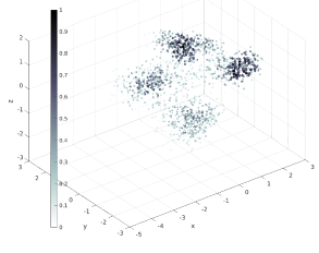
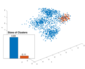
(a) density	(b) Gaussian kernel, 2 clusters
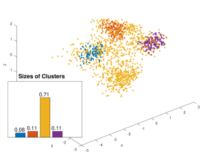
(c) Gaussian kernel, 4 clusters	(d) $K\!N\!N$ kernel, 4 clusters

Figure 3: Breiman’s bias in clustering of images. We select 4 categories from the LabelMe dataset [30]. The last fully connected layer of the neural network in [31] gives 4096-dimensional feature vector for each image. We reduce the dimension to 5 via PCA. For visualization purposes, we obtain 3D embeddings via MDS [32]. (a) Kernel densities estimates for data points are color-coded: darker points correspond to higher density. (b,c) The result of the kernel K-means with the Gaussian kernel (1). Scott’s rule of thumb defines the bandwidth. Breiman’s bias causes poor clustering, i.e. small cluster is formed in the densest part of the data in (b), three clusters occupy few points within densest regions while the fourth cluster contains 71% of the data in (c). The normalized mutual information (NMI) in (c) is 0.38. (d) Good clustering produced by $K\!N\!N$ kernel $u_{p}$ (Example 3) gives NMI of 0.90, which is slightly better than the basic K-means (0.89).

3 Adaptive weights solving Breiman’s bias

We can use a simple modification of average association by introducing weights $w_{p}\geq 0$ for each point “error” within the equivalent kernel K-means objective (3)

$$F_{w}(S,m)\;\;=\;\;\sum_{k}\sum_{p\in S^{k}}w_{p}\|\phi_{p}-m_{k}\|^{2}.$$ (41)

Such weighting is common for K-means [23]. Similarly to Section 1.1 we can expand the Euclidean distances in (41) to obtain an equivalent weighted average association criterion generalizing (9)

$$-\sum_{k}\frac{\sum_{pq\in S_{k}}w_{p}w_{q}A_{pq}}{\sum_{p\in S_{k}}w_{p}}.$$ (42)

Weights $w_{p}$ have an obvious interpretation based on (41); they change the data by replicating each point $p$ by a number of points in the same location (Figure 4a) in proportion to $w_{p}$. Therefore, this weighted formulation directly modifies the data density as

$$\rho^{\prime}_{p}\propto w_{p}\rho_{p}$$ (43)

where $\rho_{p}$ and $\rho^{\prime}_{p}$ are respectively the densities of the original and the new (replicated) points. The choice of $w_{p}=1/\rho_{p}$ is a simple way for equalizing data density to solve Breiman’s bias. As shown in Figure 4(a), such a choice enables low-density points to be replicated more frequently than high-density ones. This is one of density equalization approaches giving the solution in Figure 1(d).

- original data     - replicated data	- original data     - transformed data
(a) adaptive weights (Sec. 3)	(b) adaptive kernels (Sec. 4.3)

Figure 4: Density equalization via (a) adaptive weights and (b) adaptive kernels. In (a) the density is modified as in (43) via “replicating” each data point inverse-proportionately to the observed density using $w_{p}\propto 1/\rho_{p}$. For simplicity (a) assumes positive integer weights $w_{p}$. In (b) the density is modified according to (58) for bandwidth (61) via implicit embedding of data points in a higher dimensional space that changes their relative positions.

4 Adaptive kernels solving Breiman’s bias

Breiman’s bias in kernel K-means is specific to $r$-small bandwidths. Thus, it has direct implications for the bandwidth selection problem discussed in this section. Note that kernel bandwidth selection for clustering should not be confused with kernel bandwidth selection for density estimation, an entirely different problem outlined in Section 1.1.2. In fact, $r$-small bandwidths give accurate density estimation, but yield poor clustering due to Breiman’s bias. Larger bandwidths can avoid this bias in clustering. However, Section 4.1 shows that for extremely large bandwidths kernel K-means reduces to standard K-means, which loses ability of non-linear cluster separation and has a different bias to equal cardinality clusters [24, 27].

In practice, avoiding extreme bandwidths is problematic since the notions of small and large strongly depend on data properties that may significantly vary across the domain, e.g. in Figure 1c,d where no fixed bandwidth gives a reasonable separation. This motivates locally adaptive strategies. Interestingly, Section 4.2 shows that any locally adaptive bandwidth strategy implicitly corresponds to some data embedding $\Omega\to\mathcal{R}^{N^{\prime}}$ deforming density of the points. That is, locally adaptive selection of bandwidth is equivalent to selection of density transformation. Local kernel bandwidth and transformed density are related via the density law established in (59). As we already know from Theorem 2, Breiman’s bias is caused by high non-uniformity of the data, which can be addressed by density equalizing transformations. Section 4.3 proposes adaptive kernel strategies based on our density law and motivated by a density equalization principle addressing Breiman’s bias. In fact, a popular locally adaptive kernel in [12] is a special case of our density equalization principle.

4.1 Overview of extreme bandwidth cases

Section 2.1 and Theorem 2 prove that for $r$-small bandwidths the kernel K-means is biased toward “tight” clusters, as illustrated in Figures 1, 2 and 7(d). As bandwidth increases, continuous kernel density (11) no longer approximates the true distribution $\rho^{s}_{k}$ violating (24). Thus, Gini criterion (25) is no longer valid as an approximation for kernel K-means objective (15). In practice, Breiman’s bias disappears gradually as bandwidth gets larger. This is also consistent with experimental comparison of smaller and larger bandwidths in [3].

The other extreme case of bandwidth for kernel K-means comes from its reduction to basic K-means for large kernels. For simplicity, assume Gaussian kernels (1) of large bandwidth $\sigma$ approaching data diameter. Then the kernel can be approximated by its Taylor expansion $\exp\left(-\frac{\|x-y\|^{2}}{2\sigma^{2}}\right)\approx 1-\frac{\|x-y\|^{2}}{2\sigma^{2}}$ and kernel K-means objective (8) for $\sigma\gg\|x-y\|$ becomes (up to a constant)

$$\sum_{k}\frac{\sum_{pq\in S^{k}}\|f_{p}-f_{q}\|^{2}}{2\sigma^{2}|S^{k}|}\;\;\mbox{$\;\overset{c}{=}\;$}\;\;\frac{1}{\sigma^{2}}\;\;\sum_{k}\sum_{p\in S^{k}}\|f_{p}-m_{k}\|^{2},$$ (44)

which is equivalent to basic K-means (2) for any fixed $\sigma$.

Figure 5: Kernel K-means biases over the range of bandwidth $\sigma$. Data diameter is denoted by $d_{\Omega}=\max_{pq\in\Omega}\|f_{p}-f_{q}\|$. Breiman’s bias is established for $r$-small $\sigma$ (Section 1.1.2). Points stop interacting for $\sigma$ smaller than $r$-small making kernel K-means fail. Larger $\sigma$ reduce kernel K-means to the basic K-means removing an ability to separate the clusters non-linearly. In practice, there could be no intermediate good $\sigma$. In the example of Fig.1(c) any fixed $\sigma$ leads to either Breiman’s bias or to the lack of non-linear separability.

Figure 5 summarizes kernel K-means biases for different bandwidths. For large bandwidths the kernel K-means loses its ability to find non-linear cluster separation due to reduction to the basic K-means. Moreover, it inherits the bias to equal cardinality clusters, which is well-known for the basic K-means [24, 27]. On the other hand, for small bandwidths kernel K-means has Breiman’s bias proven in Section 2. To avoid the biases in Figure 5, kernel K-means should use a bandwidth neither too small nor too large. This motivates locally adaptive bandwidths.

4.2 Adaptive kernels as density transformation

This section shows that kernel clustering (8) with any locally adaptive bandwidth strategy satisfying some reasonable assumptions is equivalent to fixed bandwidth kernel clustering in a new feature space (Theorem 3) with a deformed point density. The adaptive bandwidths relate to density transformations via density law (59). To derive it, we interpret adaptiveness as non-uniform variation of distances across the feature space. In particular, we use a general concept of geodesic kernel defining adaptiveness via a metric tensor and illustrate it by simple practical examples.

Our analysis of Breiman’s bias in Section 2 applies to general kernels (12) suitable for density estimation. Here we focus on clustering with kernels based on radial basis functions $\psi$ s.t.

$$\mbox{$\psi$}(x-y)=\mbox{$\psi$}(\|x-y\|).$$ (45)

To obtain adaptive kernels, we replace Euclidean metric with Riemannian inside (45). In particular, $\|x-y\|$ is replaced with geodesic distances $d_{g}(x,y)$ between features $x,y\in{\cal R}^{N}$ based on any given metric tensor $g(f)$ for $f\in{\cal R}^{N}$. This allows to define a geodesic or Riemannian kernel at any points $f_{p}$ and $f_{q}$ as in [10]

$$k_{g}(f_{p},f_{q})\;\;:=\;\;\mbox{$\psi$}(d_{g}(f_{p},f_{q}))\;\;\equiv\;\;\mbox{$\psi$}(d_{pq})$$ (46)

where $d_{pq}:=d_{g}(f_{p},f_{q})$ is introduced for shortness.

In practice, the metric tensor can be defined only at the data points $g_{p}:=g(f_{p})$ for $p\in\Omega$. Often, quickly decaying radial basis functions $\psi$ allow Mahalanobis distance approximation inside (46)

$$d_{g}(f_{p},x)^{2}\;\;\approx\;\;(f_{p}-x)^{T}g_{p}\,(f_{p}-x),$$ (47)

which is normally valid only in a small neighborhood of $f_{p}$. If necessary, one can use more accurate approximations for $d_{g}(f_{p},f_{q})$ based on Dijkstra [33] or Fast Marching method [34].

Example 1 (Adaptive non-normalized Gaussian kernel).

Mahalanobis distances based on (adaptive) bandwidth matrices $\Sigma_{p}$ defined at each point $p$ can be used to define adaptive kernel

$$\kappa_{p}(f_{p},f_{q})\;:=\;\exp\frac{-(f_{p}-f_{q})^{T}\Sigma^{-1}_{p}(f_{p}-f_{q})}{2},$$ (48)

which equals fixed bandwidth Gaussian kernel (1) for $\Sigma_{p}=\sigma^{2}I$. Kernel (48) approximates (46) for exponential function $\psi$ in (13) and tensor $g$ continuously extending matrices $\Sigma^{-1}_{p}$ over the whole feature space so that $g_{p}=\Sigma^{-1}_{p}$ for $p\in\Omega$. Indeed, assuming matrices $\Sigma^{-1}_{p}$ and tensor $g$ change slowly between points within bandwidth neighbourhoods, one can use (47) for all points in

$$\kappa_{p}(f_{p},f_{q})\;\;\approx\;\;\exp\frac{-d_{g}(f_{p},f_{q})^{2}}{2}\;\;\equiv\;\;\exp\frac{-d^{2}_{pq}}{2}$$ (49)

due to exponential decay outside the bandwidth neighbourhoods.

Example 2 (Zelnik-Manor & Perona kernel [12]).

This popular kernel is defined as $\kappa_{pq}:=\exp\frac{-\|f_{p}-f_{q}\|^{2}}{2\sigma_{p}\sigma_{q}}$. This kernel’s relation to (46) is less intuitive due to the lack of “local” Riemannian tensor. However, under assumptions similar to those in (49), it can still be seen as an approximation of geodesic kernel (46) for some tensor $g$ such that $g_{p}=\sigma_{p}^{-2}I$ for $p\in\Omega$. They use heuristic $\sigma_{p}=R_{p}^{K}$, which is the distance to the K-th nearest neighbour of $f_{p}$.

Example 3 (KNN kernel).

This adaptive kernel is defined as $u_{p}(f_{p},f_{q})=[f_{q}\in\mbox{$K\!N\!N$}(f_{p})]$ where $\mbox{$K\!N\!N$}(f_{p})$ is the set of $K$ nearest neighbors of $f_{p}$. This kernel approximates (46) for uniform function $\psi(t)=[t<1]$ and tensor $g$ such that $g_{p}=I/(R^{K}_{p})^{2}$.

(a) space of points $f$	(b) transformed points $f^{\prime}$
with Riemannian metric $g$	with Euclidean metric
unit balls in Riemannian metric	unit balls in Euclidean metric

Figure 6: Adaptive kernel (46) based on Riemannian distances (a) is equivalent to fixed bandwidth kernel after some quasi-isometric (50) embedding into Euclidean space (b), see Theorem 3, mapping ellipsoids (52) to balls (54) and modifying data density as in (57).

Theorem 3.

Clustering (8) with (adaptive) geodesic kernel (46) is equivalent to clustering with fixed bandwidth kernel $k^{\prime}(f^{\prime}_{p},f^{\prime}_{q}):=\psi^{\prime}(\|f^{\prime}_{p}-f^{\prime}_{q}\|)$ in new feature space $\mathcal{R}^{N^{\prime}}$ for some radial basis function $\psi^{\prime}$ using the Euclidean distance and some constant $N^{\prime}$.

Proof.

A powerful general result in [35, 36, 15] states that for any symmetric matrix $(d_{pq})$ with zeros on the diagonal there is a constant $h$ such that squared distances

$$\widetilde{d}_{pq}^{2}\;\;=\;\;d^{2}_{pq}+h^{2}[p\neq q]$$ (50)

form Euclidean matrix $(\widetilde{d}_{pq})$. That is, there exists some Euclidean embedding $\Omega\to{\cal R}^{N^{\prime}}$ where for $\forall p\in\Omega$ there corresponds a point $f^{\prime}_{p}\in{\cal R}^{N^{\prime}}$ such that $\|f^{\prime}_{p}-f^{\prime}_{q}\|=\widetilde{d}_{pq}$, see Figure 6. Therefore,

$$\psi(d_{pq})\;\;=\;\;\psi\left(\sqrt{\widetilde{d}_{pq}^{2}-h^{2}\,[d_{pq}\geq h]}\right)\;\;\equiv\;\;\psi^{\prime}(\widetilde{d}_{pq})$$ (51)

for $\psi^{\prime}(t)\!:=\!\psi(\sqrt{t^{2}-h^{2}[t\geq h]})$ and $k_{g}(f_{p},f_{q})\!=\!k^{\prime}(f^{\prime}_{p},f^{\prime}_{q})$. ∎

Theorem 3 proves that adaptive kernels for $\{f_{p}\}\subset{\cal R}^{N}$ can be equivalently replaced by a fixed bandwidth kernel for some implicit embedding $\{f^{\prime}_{p}\}\subset{\cal R}^{N^{\prime}}$ in a new space. Below we establish a relation between three local properties at point $p\,$: adaptive bandwidth represented by matrix $g_{p}$ and two densities $\rho_{p}$ and $\rho^{\prime}_{p}$ in the original and the new feature spaces. For $\varepsilon>0$ consider an ellipsoid in the original space $\mathcal{R}^{N}$, see Figure 6(a),

$$B_{p}\;\;:=\;\;\{x\;|\;(x-f_{p})^{T}g_{p}\,(x-f_{p})\leq\varepsilon^{2}\}.$$ (52)

Assuming $\varepsilon$ is small enough so that approximation (47) holds, ellipsoid (52) covers features $\{f_{q}\,|\,q\in\Omega_{p}\}$ for subset of points

$$\Omega_{p}\;:=\;\;\{q\in\Omega\;|\;d_{pq}\leq\varepsilon\}.$$ (53)

Similarly, consider a ball in the new space $\mathcal{R}^{N^{\prime}}$, see Figure 6(b),

$$B^{\prime}_{p}\;\;:=\;\;\{x\;|\;\|x-f^{\prime}_{p}\|^{2}\leq\varepsilon^{2}+h^{2}\}$$ (54)

covering features $\{f^{\prime}_{q}\,|\,q\in\Omega^{\prime}_{p}\}$ for points

$$\Omega^{\prime}_{p}\;\;:=\;\;\{q\in\Omega\;|\;\widetilde{d}^{2}_{pq}\leq\varepsilon^{2}+h^{2}\}.$$ (55)

It is easy to see that (50) implies $\Omega_{p}=\Omega^{\prime}_{p}$. Let $\rho_{p}$ and $\rho^{\prime}_{p}$ be the densities of points within $B_{p}$ and $B^{\prime}_{p}$ correspondingly. Assuming $|\cdot|$ denotes volumes or cardinalities of sets, we have

$$\rho_{p}\cdot|B_{p}|\;\;=\;\;|\Omega_{p}|\;\;=\;\;|\Omega^{\prime}_{p}|\;\;=\;\;\rho^{\prime}_{p}\cdot|B^{\prime}_{p}|.$$ (56)

Omitting a constant factor depending on $\varepsilon$, $h$, $N$ and $N^{\prime}$ we get

$$\rho^{\prime}_{p}\;\;=\;\;\rho_{p}\;\frac{|B_{p}|}{|B^{\prime}_{p}|}\;\;\propto\;\;\rho_{p}\;|\!\det g_{p}|^{-\frac{1}{2}}$$ (57)

representing the general form of the density law. For the basic isotropic metric tensor such that $g_{p}=I/\sigma_{p}^{2}$ it simplifies to

$$\rho^{\prime}_{p}\;\;\propto\;\;\rho_{p}\,\sigma_{p}^{N}.$$ (58)

Thus, bandwidth $\sigma_{p}$ can be selected adaptively based on any desired transformation of density $\rho^{\prime}_{p}\equiv\tau(\rho_{p})$ using

$$\sigma_{p}\;\;\propto\;\;\sqrt[N]{\tau(\rho_{p})/\rho_{p}}.$$ (59)

where observed density $\rho_{p}$ in the original feature space can be evaluated at any point $p$ using any standard estimators, e.g. (11).

4.3 Density equalizing locally adaptive kernels

Bandwidth formula (59) works for any density transform $\tau$. To address Breiman’s bias, one can use density equalizing transforms $\tau(\rho)=\mbox{$\mathit{const}$}$ or $\tau(\rho)=\frac{1}{\alpha}\log(1+\alpha\rho)$, which even up

the highly dense parts of the feature space as illustrated on the right. Some empirical results using density equalization $\tau(\rho)=\mbox{$\mathit{const}$}$ for synthetic and real data are shown in Figures 1(d) and 7(e,f).

using fixed width kernel		using adaptive kernel
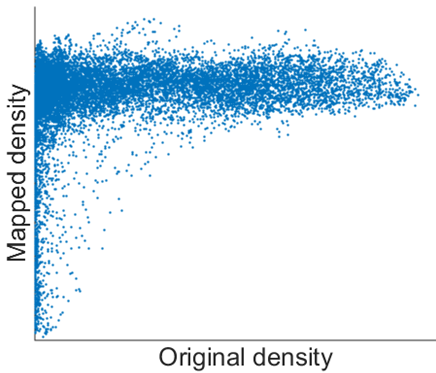
(a) input image	(b) 2D color histogram	(e) density mapping
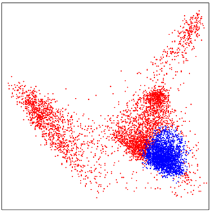
(c) clustering result	(d) color coded result	(f) clustering result

Figure 7: (a)-(d): Breiman’s bias for fixed bandwidth kernel (1). (f): result for (48) with adaptive bandwidth (61) s.t. $\tau(\rho)\!=\mbox{$\mathit{const}$}$. (e) density equalization: scatter plot of empirical densities in the original/new feature spaces obtained via (11) and (50).

One way to estimate the density in (59) is $K\!N\!N$ approach [18]

$$\rho_{p}\;\;\approx\;\;\frac{K}{nV_{K}}\;\;\propto\;\;\frac{K}{n(R_{p}^{K})^{N}}$$ (60)

where $n\equiv|\Omega|$ is the size of the dataset, $R_{p}^{K}$ is the distance to the $K$-th nearest neighbor of $f_{p}$, $V_{K}$ is the volume of a ball of radius $R_{p}^{K}$ centered at $f_{p}$. Then, density law (59) for $\tau(\rho)=\mbox{$\mathit{const}$}$ gives

$$\sigma_{p}\;\;\propto\;\;R_{p}^{K}$$ (61)

consistent with heuristic bandwidth in [12], see Example 2.

The result in Figure 1(d) uses adaptive Gaussian kernel (48) for $\Sigma_{p}=\sigma_{p}I$ with $\sigma_{p}$ derived in (61). Theorem 3 claims equivalence to a fixed bandwidth kernel in some transformed higher-dimensional space $\mathcal{R}^{N^{\prime}}\!$. Bandwidths (61) are chosen specifically to equalize the data density in this space so that $\tau(\rho)=\mbox{$\mathit{const}$}$.

The picture on the right illustrates such density equalization for the data in Figure 1(d). It shows a 3D projection of the transformed data obtained by multi-dimensional scaling [32] for matrix $(\widetilde{d}_{pq})$ in (50). The observed density equalization removes Breiman’s bias from the clustering in Figure 1(d).

Real data experiments for kernels with adaptive bandwidth (61) are reported in Figures 2, 3, 7, 8 and Table I. Figure 7(e) illustrates the empirical density equalization effect for this bandwidth. Such data homogenization removes the conditions leading to Breiman’s bias, see Theorem 2. Also, we observe empirically that $K\!N\!N$ kernel is competitive with adaptive Gaussian kernels, but its sparsity gives efficiency and simplicity of implementation.

Figure 8: Representative interactive segmentation results. Regularized average association (AA) with fixed bandwidth kernel (1) or adaptive $K\!N\!N$ kernels (Example 3) is optimized as in [37]. Red boxes define initial clustering, green contours define ground-truth clustering. Table I provides the error statistics. Breiman’s bias manifests itself by isolating the most frequent color from the rest.

regularization	average error, %
(boundary smoothness)	Gaussian AA	Gaussian NC	$K\!N\!N$ AA	$K\!N\!N$ NC
none†	20.4	17.6	12.2	12.4
Euclidean length∗	15.1	16.0	10.2	11.0
contrast-sensitive∗	9.7	13.8	7.1	7.8

TABLE I: Interactive segmentation errors. AA stands for the average association, NC stands for the normalized cut. Errors are averaged over the GrabCut dataset[38], see samples in Figure 8. ^∗We use [37, 39] for a combination of Kernel K-means objective (8) with Markov Random Field (MRF) regularization terms. The relative weight of the MRF terms is chosen to minimize the average error on the dataset. ^†Without the MRF term, [37] and [39] correspond to the standard kernel K-means [7, 9].

5 Normalized Cut and Breiman’s bias

Breiman’s bias for kernel K-means criterion (8), a.k.a. average association (AA) (9), was empirically identified in [3], but our Theorem 2 is its first theoretical explanation. This bias was the main critique against AA in [3]. They also criticize graph cut [40] that “favors cutting small sets of isolated nodes”. These critiques are used to motivate normalized cut (NC) criterion (10) aiming at balanced clustering without “clumping” or “splitting”.

We do not obeserve any evidence of the mode isolation bias in NC. However, Section 5.1 demonstrates that NC still has a bias to isolating sparse subsets. Moreover, using the general density analysis approach introduced in Section 4.2 we also show in Section 5.2 that normalization implicitly corresponds to some density-inverting embedding of the data. Thus, mode isolation (Breiman’s bias) in this implicit embedding corresponds to the sparse subset bias of NC in the original data.

5.1 Sparse subset bias in Normalized Cut

The normalization in NC does not fully remove the bias to small isolated subsets and it is easy to find examples of “splitting” for weakly connected nodes, see Figure 9(a). The motivation argument for the NC objective below Fig.1 in [3] implicitly assumes similarity matrices with zero diagonal, which excludes many common similarities like Gaussian kernel (1). Moreover, their argument is built specifically for an example with a single isolated point, while an isolated pair of points will have a near-zero NC cost even for zero diagonal similarities.

Intuitively, this NC issue can be interpreted as a bias to the “sparsest” subset (Figure 9a), the opposite of AA’s bias to the “densest” subset, i.e. Breiman’s bias (Figure 1c). The next subsection discusses the relation between these opposite biases in detail. In any case, both of these density inhomogeneity problems in NC and AA are directly addressed by our density equalization principle embodied in adaptive weights $w_{p}\propto 1/\rho_{p}$ in Section 3 or in the locally adaptive kernels derived in Section 4.3. Indeed, the result in Figure 1(d) can be replicated with NC using such adaptive kernel. Interestingly, [12] observed another data non-homogeneity problem in NC different from the sparse subset bias in Figure 9(a), but suggested a similar adaptive kernel as a heuristic solving it.

(a) NC for smaller bandwidth	(b) NC for larger bandwidth
(bias to “sparsest” subsets)	(loss of non-linear separation)

Figure 9: Normalized Cut with kernel (1) on the same data as in Figure 1(c,d). For small bandwidths NC shows bias to small isolated subsets (a). As bandwidth increases, the first non-trivial solution overcoming this bias (b) requires bandwidth large enough so that problems with non-linear separation become visible. Indeed, for larger bandwidths the node degrees become more uniform $d_{p}\approx\mbox{$\mathit{const}$}$ reducing NC to average association, which is known to degenerate into basic K-means (see Section 4.1). Thus, any further increase of $\sigma$ leads to solutions even worse than (b). In this simple example no fixed $\sigma$ leads NC to a good solution as in Figure 1(d). That good solution uses adaptive kernel from Section 4.3 making specific clustering criterion (AA, NC, or AC) irrelevant, see (68).

5.2 Normalization as density inversion

The bias to sparse clusters in NC with small bandwidths (Figure 9a) seems the opposite of mode isolation in AA (Figure 1c). Here we show that this observation is not a coincidence since NC can be reduced to AA after some density-inverting data transformation. While it is known [17, 7] that NC is equivalent to weighted kernel K-means (i.e. weighted AA) with some modified affinity, this section relates such kernel modification to an implicit density-inverting embedding where mode isolation (Breiman’s bias) corresponds to sparse clusters in the original data.

First, consider standard weighted AA objective for any given affinity/kernel matrix $\hat{A}_{pq}=k(f_{p},f_{q})$ as in (42)

$$-\sum_{k}\frac{\sum_{pq\in S_{k}}w_{p}w_{q}\hat{A}_{pq}}{\sum_{p\in S_{k}}w_{p}}.$$

Clearly, weights based on node degrees $w=d$ and “normalized” affinities $\hat{A}_{pq}=\frac{A_{pq}}{d_{p}d_{q}}$ turn this into NC objective (10). Thus, average association (9) becomes NC (10) after two modifications:

• replacing $A_{pq}$ by normalized affinities $\hat{A}_{pq}=\frac{A_{pq}}{d_{p}d_{q}}$ and

• introducing point weights $w_{p}=d_{p}$.

Both of these modifications of AA can be presented as implicit data transformations modifying denisty. In particular, we show that the first one “inverses” density turning sparser regions into denser ones, see Figure 10(a). The second data modification is generally discussed as a density transform in (43). We show that node degree weights $w_{p}=d_{p}$ do not remove the “density inversion”.

(a) density transform (65)	(b) density transform (66)
(kernel normalization only)	(with additional point weighting)

Figure 10: “Density inversion” in sparse regions. Using node degree approximation $d_{p}\propto\rho_{p}$ (67) we show representative density transformation plots (a) $\bar{\rho}_{p}=\tau(\rho_{p})$ and (b) $\rho^{\prime}_{p}=\tau(\rho_{p})$ corresponding to AA with kernel modification $\hat{A}_{pq}=\frac{A_{pq}}{d_{p}d_{q}}$ (65) and additional point weighting $w_{p}=d_{p}$ (66) exactly corresponding to NC. This additional weighting weakens the density inversion in (b) compared to (a), see the $x$-axis scale difference. However, it is easy to check that the minima in (65) and (66) are achieved at some $x^{*}$ exponentially growing with $\bar{N}$. This makes the density inversion significant for NC since $\bar{N}$ may equal the data size.

For simplicity, assume standard Gaussian kernel (1) based on Euclidean distances $d_{pq}=\|f_{p}-f_{q}\|$ in $\mathcal{R}^{N}$

$$A_{pq}=\exp\frac{-d^{2}_{pq}}{2\sigma^{2}}.$$

To convert AA into NC we first need an affinity “normalization”

$$\hat{A}_{pq}=\frac{A_{pq}}{d_{p}d_{q}}=\exp\frac{-d^{2}_{pq}-2\sigma^{2}\log(d_{p}d_{q})}{2\sigma^{2}}=\exp\frac{-\hat{d}^{2}_{pq}}{2\sigma^{2}}$$ (62)

equivalently formulated as a modification of distances

$$\hat{d}^{2}_{pq}\;\;:=\;\;d^{2}_{pq}+2\sigma^{2}\log(d_{p}d_{q}).$$ (63)

Using a general approach in the proof of Theorem 3, there exists some Euclidean embedding $\bar{f}_{p}\in\mathcal{R}^{\bar{N}}$ and constant $h\geq 0$ such that

$$\bar{d}^{2}_{pq}\;\;:=\;\;\|\bar{f}_{p}-\bar{f}_{q}\|^{2}\;\;=\;\;\hat{d}^{2}_{pq}+h^{2}[p\neq q].$$ (64)

Thus, modified affinities $\hat{A}_{pq}$ in (62) correspond to the Gaussian kernel for the new embedding $\{\bar{f}_{p}\}$ in $\mathcal{R}^{\bar{N}}$

$$\hat{A}_{pq}\;\;\propto\;\;\exp\frac{-\bar{d}^{2}_{pq}}{2\sigma^{2}}\;\;\equiv\;\;\exp\frac{-\|\bar{f}_{p}-\bar{f}_{q}\|^{2}}{2\sigma^{2}}.$$

Assuming $d_{q}\approx d_{p}$ for features $f_{q}$ near $f_{p}$, equations (63) and (64) imply the following relation for such neighbors of $f_{p}$

$$\bar{d}^{2}_{pq}\;\;\approx\;\;d^{2}_{pq}+h^{2}+4\sigma^{2}\log(d_{p}).$$

Then, similarly to the arguments in (56), a small ball of radius $\varepsilon$ centered at $f_{p}$ in $\mathcal{R}^{N}$ and a ball of radius $\sqrt{\varepsilon^{2}+h^{2}+4\sigma^{2}\log(d_{p})}$ at $\bar{f}_{p}$ in $\mathcal{R}^{\bar{N}}$ contain the same number of points. Thus, similarly to (57) we get a relation between densities at points $f_{p}$ and $\bar{f}_{p}$

$$\bar{\rho}_{p}\;\;\approx\;\;\frac{\rho_{p}\;\varepsilon^{N}}{(\varepsilon^{2}+h^{2}+4\sigma^{2}\log(d_{p}))^{\bar{N}/2}}.$$ (65)

This implicit density transformation is shown in Figure 10(a). Sub-linearity in dense regions addresses mode isolation (Breiman’s bias). However, sparser regions become relatively dense and kernel-modified AA may split them. Indeed, the result in Figure 9(a) can be obtained by AA with normalized affinity $\frac{A_{pq}}{d_{p}d_{q}}$.

	(a) original data $\{f_{p}\}\subset\mathcal{R}^{1}$	(b) embedding $\{\bar{f}_{p}\}\subset\mathcal{R}^{\bar{N}}$

Figure 11: Illustration of “density inversion” for 1D data. The original data points (a) are getting progressively denser along the line. The points are color-coded according to the log of their density. Plot (b) shows 3D approximation $\{y_{p}\}\subset\mathcal{R}^{3}$ of high-dimensional Euclidean embedding $\{\bar{f}_{p}\}\subset\mathcal{R}^{\bar{N}}$ minimizing metric errors $\sum_{pq}(\hat{d}^{2}_{pq}-\|y_{p}-y_{q}\|^{2})^{2}$ where $\hat{d}_{pq}$ are distances (63).

The second required modification of AA introduces point weights $w_{p}=d_{p}$. It has an obvious equivalent formulation via data points replication discussed in Section 3, see Figure 4(a). Following (43), we obtain its implicit density modification effect $\rho^{\prime}_{p}=d_{p}\bar{\rho}_{p}$. Combining this with density transformation (65) implied by affinity normalization $\frac{A_{pq}}{d_{p}d_{q}}$, we obtain the following density transformation effect corresponding to NC, see Figure 10(b),

$$\rho^{\prime}_{p}\;\;\approx\;\;\frac{d_{p}\;\rho_{p}\;\varepsilon^{N}}{(\varepsilon^{2}+h^{2}+4\sigma^{2}\log(d_{p}))^{\bar{N}/2}}.$$ (66)

The density inversion in sparse regions relates NC’s result in Figure 9(a) to Breiman’s bias for embedding $\{\bar{f}_{p}\}$ in $\mathcal{R}^{\bar{N}}$.

Figure 10 shows representative plots for density transformations (65), (66) using the following node degree approximation based on Parzen approach (11) for Gaussian affinity (kernel) $A$

$$d_{p}=\sum_{q}A_{pq}\propto\rho_{p}.$$ (67)

Empirical relation between $d_{p}$ and $\rho_{p}$ is illistrated below: some

overestimation occurs for sparcer regions and underestimation happens for denser regions. The node degree for Gaussian kernels has to be at least $1$ (for an isolated node) and at most $N$ (for a dense graph).

6 Discussion (kernel clustering equivalence)

Density equalization with adaptive weights in Section 3 or adaptive kernels in Section 4 are useful for either AA or NC due to their density biases (mode isolation or sparse subset). Interestingly, kernel clustering criteria discussed in [3] such as normalized cut (NC), average cut (AC), average association (AA) or kernel K-means are practically equivalent for such adaptive methods. This can be seen both empirically (Table I) and conceptually. Note, weights $w_{p}\propto 1/\rho_{p}$ in Section 3 produce modified data with near constant node degrees $d^{\prime}_{p}\propto\rho^{\prime}_{p}\propto 1$, see (67) and (43). Alternatively, KNN kernel (Example 3) with density equalizing bandwidth (61) also produce nearly constant node degrees $d_{p}\approx K$ where $K$ is the neighborhood size. Therefore, both cases give

$$-\frac{\sum_{pq\in S^{k}}A_{pq}}{\sum_{p\in S^{k}}d_{p}}\;\;\propto\;\;-\frac{\sum_{pq\in S^{k}}A_{pq}}{K\,|S^{k}|}\;\;\mbox{$\;\overset{c}{\approx}\;$}\;\;\frac{\sum_{p\in S^{k},q\in\bar{S}^{k}}A_{pq}}{K\,|S^{k}|},$$ (68)

which correspond to NC (10), AA (9), and AC criteria. As discussed in [3], the last objective also has very close relations with standard partitioning concepts in spectral graph theory: isoperimetric or Cheeger number, Cheeger set, ratio cut.

This equivalence argument applies to the corresponding clustering objectives and is independent of specific optimization algorithms developed for them. Interestingly, the relation between (9) and basic K-means objective (3) suggests that standard Lloyd’s algorithm can be used as a basic iterative approach for approximate optimization of all clustering criteria in (68). In practice, however, kernel K-means algorithm corresponding to the exact high-dimensional embedding $\{\phi_{p}\}$ in (3) is more sensitive to local minima compared to iterative K-means over approximate lower-dimensional embeddings based on PCA [14, Section 3.1].

7 Conclusions

This paper identifies and proves density biases, i.e. isolation of modes or sparsest subsets, in many well-known kernel clustering criteria such as kernel K-means (average association), ratio cut, normalized cut, dominant sets. In particular, we show conditions when such biases happen. Moreover, we propose density equalization as a general principle for resolving such biases. We suggest two types of density equalization techniques using adaptive weights or adaptive kernels. We also show that density equalization unifies many popular kernel clustering objectives by making them equivalent.

Dmitrii Marin received Diploma of Specialist from the Ufa State Aviational Technical University in 2011, and M.Sc. degree in Applied Mathematics and Information Science from the National Research University Higher School of Economics, Moscow, and graduated from the Yandex School of Data Analysis, Moscow, in 2013. In 2010 obtained a certificate of achievement at ACM ICPC World Finals, Harbin. He is a PhD candidate at the Department of Computer Science, University of Western Ontario under supervision of Yuri Boykov. His research is focused on designing general unsupervised and semi-supervised methods for accurate image segmentation and object delineation.

Meng Tang is a PhD candidate in computer science at the University of Western Ontario, Canada, supervised by Prof. Yuri Boykov. He obtained MSc in computer science in 2014 from the same institution for his thesis titled ”Color Separation for Image Segmentation”. Previously in 2012 he received B.E. in Automation from the Huazhong University of Science and Technology, China. He is interested in image segmentation and semi-supervised data clustering. He is also obsessed and has experiences on discrete optimization problems for computer vision and machine learning.

Ismail Ben Ayed received the PhD degree (with the highest honor) in computer vision from the Institut National de la Recherche Scientifique (INRS-EMT), Montreal, QC, in 2007. He is currently Associate Professor at the Ecole de Technologie Superieure (ETS), University of Quebec, where he holds a research chair on Artificial Intelligence in Medical Imaging. Before joining the ETS, he worked for 8 years as a research scientist at GE Healthcare, London, ON, conducting research in medical image analysis. He also holds an adjunct professor appointment at the University of Western Ontario (since 2012). Ismail’s research interests are in computer vision, optimization, machine learning and their potential applications in medical image analysis.

Yuri Boykov received ”Diploma of Higher Education” with honors at Moscow Institute of Physics and Technology (department of Radio Engineering and Cybernetics) in 1992 and completed his Ph.D. at the department of Operations Research at Cornell University in 1996. He is currently a full professor at the department of Computer Science at the University of Western Ontario. His research is concentrated in the area of computer vision and biomedical image analysis. In particular, he is interested in problems of early vision, image segmentation, restoration, registration, stereo, motion, model fitting, feature-based object recognition, photo-video editing and others. He is a recipient of the Helmholtz Prize (Test of Time) awarded at International Conference on Computer Vision (ICCV), 2011 and Florence Bucke Science Award, Faculty of Science, The University of Western Ontario, 2008.

References

- [1] B. Schölkopf, A. Smola, and K.-R. Müller, “Nonlinear component analysis as a kernel eigenvalue problem,” Neural computation, vol. 10, no. 5, pp. 1299–1319, 1998.
- [2] V. Vapnik, Statistical Learning Theory. Wiley, 1998.
- [3] J. Shi and J. Malik, “Normalized cuts and image segmentation,” IEEE Transactions on Pattern Analysis and Machine Intelligence, vol. 22, pp. 888–905, 2000.
- [4] K. Muller, S. Mika, G. Ratsch, K. Tsuda, and B. Scholkopf, “An introduction to kernel-based learning algorithms,” IEEE Trans. Neural Networks, vol. 12, no. 2, pp. 181–201, 2001.
- [5] R. Zhang and A. Rudnicky, “A large scale clustering scheme for kernel k-means,” in Pattern Recognition, 2002., vol. 4, 2002, pp. 289–292.
- [6] M. Girolami, “Mercer kernel-based clustering in feature space,” IEEE Trans. Neural Networks, vol. 13, no. 3, pp. 780–784, 2002.
- [7] I. Dhillon, Y. Guan, and B. Kulis, “Kernel k-means, spectral clustering and normalized cuts,” in KDD, 2004.
- [8] M. Pavan and M. Pelillo, “Dominant sets and pairwise clustering,” IEEE Transactions on Pattern Analysis and Machine Intelligence, vol. 29, no. 1, pp. 167–172, 2007.
- [9] R. Chitta, R. Jin, T. Havens, and A. Jain, “Scalable kernel clustering: Approximate kernel k-means,” in KDD, 2011, pp. 895–903.
- [10] S. Jayasumana, R. Hartley, M. Salzmann, H. Li, and M. Harandi, “Kernel methods on Riemannian manifolds with Gaussian RBF kernels,” IEEE Transactions on Pattern Analysis and Machine Intelligence (TPAMI), vol. 37, no. 12, pp. 2464–2477, 2015.
- [11] L. Breiman, “Technical note: Some properties of splitting criteria,” Machine Learning, vol. 24, no. 1, pp. 41–47, 1996.
- [12] L. Zelnik-Manor and P. Perona, “Self-tuning spectral clustering,” in Advances in NIPS, 2004, pp. 1601–1608.
- [13] D. Comaniciu and P. Meer, “Mean shift: A robust approach toward feature space analysis,” IEEE Transactions on Pattern Analysis and Machine Intelligence (PAMI), 2002.
- [14] M. Tang, D. Marin, I. B. Ayed, and Y. Boykov, “Kernel Cuts: MRF meets kernel and spectral clustering,” in arXiv:1506.07439, September 2016 (also submitted to IJCV).
- [15] V. Roth, J. Laub, M. Kawanabe, and J. Buhmann, “Optimal cluster preserving embedding of nonmetric proximity data,” IEEE Trans. Pattern Anal. Mach. Intell., vol. 25, no. 12, pp. 1540—1551, 2003.
- [16] U. Von Luxburg, “A tutorial on spectral clustering,” Statistics and computing, vol. 17, no. 4, pp. 395–416, 2007.
- [17] F. Bach and M. Jordan, “Learning spectral clustering,” Advances in Neural Information Processing Systems, vol. 16, pp. 305–312, 2003.
- [18] C. M. Bishop, Pattern Recognition and Machine Learning. Springer, August 2006.
- [19] D. W. Scott, Multivariate density estimation: theory, practice, and visualization. John Wiley & Sons, 1992.
- [20] B. W. Silverman, Density estimation for statistics and data analysis. CRC press, 1986, vol. 26.
- [21] A. J. Izenman, “Review papers: Recent developments in nonparametric density estimation,” Journal of the American Statistical Association, vol. 86, no. 413, pp. 205–224, 1991.
- [22] G. R. Terrell and D. W. Scott, “Variable kernel density estimation,” The Annals of Statistics, vol. 20, no. 3, pp. 1236–1265, 1992. [Online]. Available: http://www.jstor.org/stable/2242011
- [23] R. O. Duda and P. E. Hart, Pattern Classification and Scene Analysis. Wiley, 1973.
- [24] M. Kearns, Y. Mansour, and A. Ng, “An Information-Theoretic Analysis of Hard and Soft Assignment Methods for Clustering,” in Conf. on Uncertainty in Artificial Intelligence (UAI), August 1997.
- [25] C. Fraley and A. E. Raftery, “Model-Based Clustering, Discriminant Analysis, and Density Estimation,” Journal of the American Statistical Association, vol. 97, no. 458, pp. 611–631, 2002.
- [26] A. Criminisi and J. Shotton, Decision Forests for Computer Vision and Medical Image Analysis. Springer, 2013.
- [27] Y. Boykov, H. Isack, C. Olsson, and I. B. Ayed, “Volumetric Bias in Segmentation and Reconstruction: Secrets and Solutions,” in International Conference on Computer Vision (ICCV), December 2015.
- [28] L. Breiman, J. Friedman, C. J. Stone, and R. A. Olshen, Classification and regression trees. CRC press, 1984.
- [29] T. S. Motzkin and E. G. Straus, “Maxima for graphs and a new proof of a theorem of turán,” Canad. J. Math, vol. 17, no. 4, pp. 533–540, 1965.
- [30] A. Oliva and A. Torralba, “Modeling the shape of the scene: A holistic representation of the spatial envelope,” International journal of computer vision, vol. 42, no. 3, pp. 145–175, 2001.
- [31] A. Krizhevsky, I. Sutskever, and G. E. Hinton, “Imagenet classification with deep convolutional neural networks,” in Advances in neural information processing systems, 2012, pp. 1097–1105.
- [32] T. Cox and M. Cox, Multidimensional scaling. CRC Press, 2000.
- [33] T. H. Cormen, C. E. Leiserson, R. L. Rivest, and C. Stein, Introduction to algorithms. MIT press, 2006.
- [34] J. A. Sethian, Level set methods and fast marching methods. Cambridge university press, 1999, vol. 3.
- [35] J. Lingoes, “Some boundary conditions for a monotone analysis of symmetric matrices,” Psychometrika, 1971.
- [36] J. C. Gower and P. Legendre, “Metric and euclidean properties of dissimilarity coefficients,” Journal of classification, vol. 3, no. 1, pp. 5–48, 1986.
- [37] M. Tang, I. B. Ayed, D. Marin, and Y. Boykov, “Secrets of grabcut and kernel k-means,” in International Conference on Computer Vision (ICCV), Santiago, Chile, December 2015.
- [38] C. Rother, V. Kolmogorov, and A. Blake, “Grabcut - interactive foreground extraction using iterated graph cuts,” in ACM trans. on Graphics (SIGGRAPH), 2004.
- [39] M. Tang, D. Marin, I. B. Ayed, and Y. Boykov, “Normalized Cut meets MRF,” in European Conference on Computer Vision (ECCV), 2016.
- [40] Z. Wu and R. Leahy, “An optimal graph theoretic approach to data clustering: theory and its application to image segmentation,” IEEE Trans. Pattern Anal. Mach. Intell., vol. 15, no. 11, pp. 1101–1113, Nov 1993.
- [41] J. Cheeger, “A lower bound for the smallest eigenvalue of the laplacian,” Problems in Analysis, R.C. Gunning, ed., pp. 195–199, 1970.
- [42] W. Donath and A. Hoffman, “Lower bounds for the partitioning of graphs,” IBM J. Research and Development, pp. 420–425, 1973.
- [43] M. Fiedler, “A property of eigenvectors of nonnegative symmetric matrices and its applications to graph theory,” Czech. Math. J., vol. 25, no. 100, pp. 619–633, 1975.