Invariance of topological indices under Hilbert space truncation

Abstract

We show that the topological index of a wavefunction, computed in the space of twisted boundary phases, is preserved under Hilbert space truncation, provided the truncated state remains normalizable. If truncation affects the boundary condition of the resulting state, the invariant index may acquire a different physical interpretation. If the index is symmetry protected, the truncation should preserve the protecting symmetry. We discuss implications of this invariance using paradigmatic integer and fractional Chern insulators, $Z_{2}$ topological insulators, and Spin-$1$ AKLT and Heisenberg chains, as well as its relation with the notion of bulk entanglement. As a possible application, we propose a partial quantum tomography scheme from which the topological index of a generic multi-component wavefunction can be extracted by measuring only a small subset of wavefunction components, equivalent to the measurement of a bulk entanglement topological index.

Introduction

The investigation of topological phases and their classification Bernevig and Hughes (2013); Qi and Zhang (2011); Ryu et al. (2010); Chiu et al. (2016) has grown into a major endeavor in condensed matter physics, thanks to rapid advancements in material realization Hasan and Kane (2010); Ando (2013) and experimental platforms for “quantum simulation” such as ultra cold atomic systems Bloch et al. (2008, 2012); Langen et al. (2015). The appeal of topology is that related physical quantities, for example quantized Hall conductance Thouless et al. (1982) and charge polarization Zak (1989); King-Smith and Vanderbilt (1993), can be formulated as discrete topological indices, which are thus robust against continuous deformations of the system.

A topological index is fundamentally a property of a wavefunction. Yet apart from free fermions and a few exactly solvable models, it is impractical to obtain an exact wavefunction through the diagonalization of a Hamiltonian. One alternative is to build candidate wavefunctions through projective construction, whereby a parent state defined in a larger Hilbert space is linked to a projected state in a smaller, truncated Hilbert space Suzuki and Lee (1980); Anderson (1987); Gros (1989). Both the parent and the truncated Hilbert spaces can play the role of the physical space. For example, a matrix product state is constructed by projecting a parent state, defined in a tensor product of site Hilbert spaces, onto bond Hilbert spaces, where truncation in bond dimension is implemented according to the entanglement content Schollwöck (2011). In this case, the parent space is physical, while the projected state offers a more economical description suitable for numerical solution. In parton-type constructions Wen (2002), on the other hand, one first fractionalizes the physical degrees of freedom into partons, with which a mean field state can be written down in the enlarged parton Hilbert space, then a Gutzwiller type projection is employed to pull the state back to the physical space. In this case, the truncated space is physical, while the enlarged space provides a more natural platform for exotic phenomena such as fractionalization. Treated as variational ansatz, the projected wavefunctions thus obtained can be further optimized for better approximation of target states, yet for the issue of topological characterization, a fundamental question remains rarely touched: how does the truncation procedure itself affect topology?

In this work, we investigate the connection between Hilbert space truncation and topology on the wavefunction level. Specifically, we address the question: what is the relation between the parent and the projected wavefunctions in terms of their topological index? The topological indices we will consider are those that can be computed via the formalism of twisted boundary phases Niu et al. (1985), such as integer and fractional Chern numbers, quantized Berry phase, and various symmetry protected $Z_{2}$ indices. We will assume that the parent state is a gapped eigenstate $|\Psi({\boldsymbol{\kappa}})\rangle$ of a many-body Hamiltonian, hence it has well-defined topological indices. Here ${\boldsymbol{\kappa}}\equiv(\kappa_{1},\kappa_{2},\cdots)$ are the boundary phases implemented as $a^{+}_{{\boldsymbol{r}}+N_{i}\hat{e}_{i}}=a^{+}_{{\boldsymbol{r}}}e^{i\kappa_{i}}$, where $a^{+}_{{\boldsymbol{r}}}$ is a fermionic/bosonic creation operator or a spin raising operator on lattice site ${\boldsymbol{r}}$, and $N_{i}$ is the linear size along direction $\hat{e}_{i}$. The full parameter space of ${\boldsymbol{\kappa}}$, with $\kappa_{i}\in[0,2\pi)\forall i$, will be referred to as a “Brillouin Zone” (BZ). We will show that the topological index of $|\Psi\rangle$ is fully preserved by its truncated version, $|\widetilde{\Psi}\rangle=P|\Psi\rangle/\sqrt{\langle\Psi|P|\Psi\rangle}$, if both indices are computed using the same ${\boldsymbol{\kappa}}$ BZ, provided the ${\boldsymbol{\kappa}}$-independent projection $P$ fulfills the following conditions: (1) At no point in the ${\boldsymbol{\kappa}}$ BZ does the truncated wavefunction become a null vector, whereby information of the parent state is fully lost. (2) For a parent state belonging to symmetry protected topological classes, the truncation should also preserve the protecting symmetry in order for the classification to remain meaningful. This is consistent with recent works on the node structure in wavefunctions overlaps Gu and Sun (2016); Huang and Balatsky (2016), and we discuss their relation and distinction in the SM. Note that under certain truncation schemes, ${\boldsymbol{\kappa}}$ may no longer correspond to physical boundary phases for the truncated state. In such cases, truncation invariance remains true mathematically, but acquires a different physical interpretation, and may place the truncated state in a different topological class from the parent state, see later discussion on the parton construction of fractional Chern insulators.

Truncation invariance of Chern number and related topological indices

We begin by constructively showing that the Chern number is invariant under Hilbert space truncation. This serves as a generic proof that any topological index obtainable from a Chern number calculation will remain invariant under such a truncation. Calculation of the Chern number is at the heart of topological classification of two-parameter-family wavefunctions. In addition to the integer and fractional quantum Hall effect Thouless et al. (1982); Kohmoto (1985); Niu et al. (1985), it can also be used to classify symmetry protected topological (SPT) states by restricting its calculation to a subset of states or a reduced parameter space, examples include spin Chern number for time-reversal-invariant TIs Sheng et al. (2006); Fukui and Hatsugai (2007); Prodan (2009); Yang et al. (2011), mirror Chern number Teo et al. (2008) and more generally Chern numbers over 2D high symmetry manifold within a 3D single particle BZ for crystalline TIs Alexandradinata et al. (2014). We will discuss its implication on fractional Chern insulator states later in the text. A step by step illustration of the proof to be discussed below can be found in the SM using a $3$-band Hofstadter model. Further examples of band Chern insulators and $Z_{2}$ TIs are also provided in the SM.

Consider a gapped eigenstate of a many-body Hamiltonian in two dimensions, $|\Psi({\boldsymbol{\kappa}})\rangle=\sum_{i=1}^{M}\Psi_{i}({\boldsymbol{\kappa}})|B_{i}\rangle$, where ${\boldsymbol{\kappa}}=(\kappa_{x},\kappa_{y})$ are twisted boundary phases, $\kappa_{x,y}\in[0,2\pi)$. $\{|B_{i}\rangle\}$ are orthonormal many-body bases independent of ${\boldsymbol{\kappa}}$, and $\Psi_{i}({\boldsymbol{\kappa}})=\langle B_{i}|\Psi({\boldsymbol{\kappa}})\rangle$ is periodic in ${\boldsymbol{\kappa}}$. The Chern number of $\Psi$ is $C=\frac{1}{2\pi}\iint_{\text{BZ}}d^{2}\kappa\,\nabla_{{\boldsymbol{\kappa}}}\times\langle\Psi|i\nabla_{{\boldsymbol{\kappa}}}|\Psi\rangle.$ We first show that $C$ can be computed using any two components of $|\Psi({\boldsymbol{\kappa}})\rangle$, say $\Psi_{i_{1}}({\boldsymbol{\kappa}})$ and $\Psi_{i_{2}}({\boldsymbol{\kappa}})$, provided they do not vanish at the same ${\boldsymbol{\kappa}}$ point(s). We adopt the gauge fixing scheme of Ref. Kohmoto (1985). Assume for simplicity that a component $\Psi_{i_{1}}({\boldsymbol{\kappa}})$ has a single zero in the entire BZ at, say, ${\boldsymbol{\kappa}}^{*}$. Cases with multiple such zeros will be discussed later. Divide the BZ into two patches, where one patch, denoted as $R_{2}$, is an infinitesimal neighborhood around ${\boldsymbol{\kappa}}^{*}$, and the remainder of the BZ is the other patch, denoted as $R_{1}$. We choose the gauge of $|\Psi\rangle$ such that

$$\Psi_{i_{a}}({\boldsymbol{\kappa}})>0\text{ for }{\boldsymbol{\kappa}}\in R_{a}\ ,\ a=1,2\ .$$ (1)

The gauge of $|\Psi\rangle$ is therefore smooth in both $R_{1}$ and $R_{2}$, but has a phase mismatch across their interface,

$$|\Psi({\boldsymbol{\kappa}}_{\cap})\rangle_{R_{1}}=e^{i\lambda({\boldsymbol{\kappa}}_{\cap})}|\Psi({\boldsymbol{\kappa}}_{\cap})\rangle_{R_{2}}\ ,\ {\boldsymbol{\kappa}}_{\cap}\in R_{1}\cap R_{2}\ ,$$ (2)

where subscripts $R_{i}$ denote gauge choice. In gauge $R_{1}$, one can write $(\Psi_{i_{1}},\Psi_{i_{2}})_{R_{1}}=(r_{1},r_{2}e^{i\chi})$ with $r_{1,2}>0$ and real $\chi$. Then under gauge $R_{2}$, $(\Psi_{i_{1}},\Psi_{i_{2}})_{R_{2}}=(r_{1}e^{-i\chi},r_{2})$. By Eq. 2, one can identify $\lambda=\chi$, viz.,

$$\lambda({\boldsymbol{\kappa}}_{\cap})=\textsf{Arg}\left[\Psi_{i_{2}}({\boldsymbol{\kappa}}_{\cap})/\Psi_{i_{1}}({\boldsymbol{\kappa}}_{\cap})\right]\ ,$$ (3)

which is gauge invariant. The BZ integral for computing $C$ is now a sum over the two patches $R_{1,2}$, and by Stokes Theorem, each patch contributes a line integral of the Berry connection vector over the patch’s boundary, thus

$$C=\frac{1}{2\pi}\sum_{i=1,2}\oint\limits_{\partial R_{i}}d{\boldsymbol{\kappa}}_{\cap}\cdot\langle\Psi|i\nabla_{{\boldsymbol{\kappa}}_{\cap}}|\Psi\rangle_{R_{i}}=w[\lambda]\ ,$$ (4)

where $w[\lambda]=\frac{1}{2\pi}\ointctrclockwise_{\,\partial R_{2}}d{\boldsymbol{\kappa}}_{\cap}\cdot\partial_{{\boldsymbol{\kappa}}_{\cap}}\lambda$ is the winding number of the phase mismatch $\lambda({\boldsymbol{\kappa}}_{\cap})$ in the counter-clockwise direction—note that the two boundaries, $\partial R_{1}$ and $\partial R_{2}$, are identical but in opposite directions. If $\Psi_{i_{1}}$ has multiple zeros, one can define a phase mismatch $\lambda_{a}$ around the $a^{th}$ zero, and $C=\sum_{a}w[\lambda_{a}]$. Eqs. 3 and 4 together establish that the Chern number of $|\Psi\rangle$ can be computed using any two of its components.

Now consider a truncated state $|\widetilde{\Psi}\rangle$ obtained by taking a subset of wavefunction components from $|\Psi\rangle$ and renormalizing. Its Chern number can be computed in the same way using $\widetilde{\Psi}_{i_{1}}$ and $\widetilde{\Psi}_{i_{2}}$. Since both are simply rescaled from their pre-truncation values, the phase mismatch (Eq. 3) is not affected by the truncation, hence $|\widetilde{\Psi}\rangle$ and $|\Psi\rangle$ have the same Chern number.

Truncation invariance of quantized Berry phase

Symmetry-protected 1D topological phases exhibit a robust $Z_{2}$ index due to the quantization of the Berry phase to either $0$ or $\pi$. We now prove the truncation invariance of the $Z_{2}$ class protected by inversion-like symmetries. Examples in this class include the Su-Schrieffer-Heeger model, Kitaev’s $p$-wave superconductor, and Spin-$1$ antiferromagnetic chain. Consider a parent many-body Hamiltonian $H(\kappa)=H(\kappa+2\pi)$, where $\kappa\in[0,2\pi)$ is the boundary phase. Inversion-like invariance is defined as $SH(\kappa)S^{-1}=H(-\kappa)$ where the unitary $S$ represents the symmetry operation. At the symmetry invariant points $\kappa_{\textsf{SIP}}\in\{0,\pi\}$, $S$ commutes with $H(\kappa_{\textsf{SIP}})$, hence the ground state of $H$, assumed unique, must also be a symmetry eigenstate, $S|\Psi(\kappa_{\textsf{SIP}})\rangle=s_{\kappa_{\textsf{SIP}}}|\Psi(\kappa_{\textsf{SIP}})\rangle$, where $s_{\kappa_{\textsf{SIP}}}=\pm 1$. Hughes et al showed Hughes et al. (2011) that the Berry phase of $|\Psi(\kappa)\rangle$ can be computed from the symmetry eigenvalues at $\kappa_{\textsf{SIP}}$, $e^{i\gamma}=s_{0}s_{\pi}$. Now consider a truncation $P$ that preserves inversion, $[P,S]=0$. It follows that the truncated state $P|\Psi(\kappa_{\textsf{SIP}})\rangle$ remains an inversion eigenstate with the same eigenvalue $s_{\kappa_{\textsf{SIP}}}$ as the parent state $|\Psi(\kappa_{\textsf{SIP}})\rangle$. Hence, the Berry phase also remains invariant, provided $P$ does not annihilate $|\Psi(\kappa)\rangle$ for any $\kappa$.

Parton construction of fractional Chern insulators

Truncation invariance of the Chern number is closely related to the parton construction of fractional Chern insulator (FCI) states McGreevy et al. (2012); Lu and Ran (2012); Zhang and Vishwanath (2013); Hu et al. (2015); Kourtis et al. (2014). Consider the $\textsf{SU}(m)$ FCI state McGreevy et al. (2012); Lu and Ran (2012), a lattice analogue of the Laughlin $\frac{1}{m}$ state. One writes the electron (or boson) operator as a product of $m$ partons, $c_{{\boldsymbol{r}}}=\prod_{\alpha=1}^{m}f_{{\boldsymbol{r}}}^{(\alpha)}$. Each parton species is subjected to a tight binding Hamiltonian with lowest band Chern number $1$. Filling one band per species then leads to a parton mean field state $|\Psi_{\text{MF}}\rangle$ with Chern number $C_{\text{MF}}=m$ by construction. The FCI state is obtained by Gutzwiller projecting $|\Psi_{\text{MF}}\rangle$ back to the electron Hilbert space, $|\Psi_{\text{el}}\rangle\propto P_{G}|\Psi_{\text{MF}}\rangle$, that is, $0$ or $m$ partons per lattice site. From truncation invariance, $|\Psi_{\text{el}}\rangle$ and $|\Psi_{\text{MF}}\rangle$ have the same Chern number over a parton BZ, $\kappa_{x,y}\in[0,2\pi)$. Here, $\kappa_{x,y}$ are parton twisted boundary phases, $f_{{\boldsymbol{r}}+N_{i}\hat{e}_{i}}^{(\alpha)}=e^{i\kappa_{i}}f^{(\alpha)}_{{\boldsymbol{r}}}$. The corresponding boundary conditions for electrons are $c_{{\boldsymbol{r}}+N_{i}\hat{e}_{i}}=\prod_{\alpha=1}^{m}f_{{\boldsymbol{r}}+N_{i}\hat{e}_{i}}^{(\alpha)}=e^{im\kappa_{i}}c_{{\boldsymbol{r}}}$, hence one parton BZ is equivalent to $m^{2}$ electron BZs. Thus although the Chern number remains invariant after truncation when computed using the parton BZ, the physical Hall conductance is related to the Chern number per electron BZ Niu et al. (1985), and we recover the fractional Hall conductance of $|\Psi_{\text{el}}\rangle$ as $C=\frac{C_{\text{MF}}}{m^{2}}=\frac{1}{m}$.

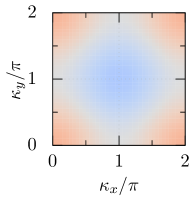
(a) Parton mean field state

(b) Bosonic FCI state

Figure 1: Chern number density in the space of parton boundary phases for (a) the parent (untruncated) parton mean-field state, and (b) the bosonic fractional Chern insulator state obtained via Gutzwiller projection. In both cases, the Chern number density integrates to the same $C_{\text{MF}}=2$ over the parton BZ, as required by truncation invariance. The physical Hall conductance of the FCI state is given by $C=\frac{C_{\text{MF}}}{m^{2}}=\frac{1}{2}$ with $m=2$ parton species, see text for detail. Calculation is done with a $4\times 4$ lattice and a $40\times 40$ grid of $(\kappa_{x},\kappa_{y})$.

In Fig. 1, we use the $\pi$-flux square lattice model of Ref. Zhang and Vishwanath (2013) as the mean field Hamiltonian for $m=2$ parton species, and plot the Chern number density for both the untruncated parton mean field state $|\Psi_{\text{MF}}\rangle$ and the bosonic FCI state obtained by Gutzwiller projecting $|\Psi_{\text{MF}}\rangle$ to $0$ or $2$ partons per site. In both cases, the Chern number density integrates to $C_{\text{MF}}=2$ over the parton BZ, as guaranteed by truncation invariance. The physical Hall conductance is given by $C=\frac{C_{\text{MF}}}{m^{2}}=\frac{1}{2}$.

We note that numerical calculations of the fractional Chern number of Gutzwiller-projected parton states are severely limited by system size Hu et al. (2015). Our theorem establishes such results on a more general ground, without system size restriction. The same argument applies to the ground states of non-Abelian FCIs as well (see SM), although its connection with quasi-particle statistics remains an open question.

Spin-$1$ antiferromagnetic chain

We use the Spin-$1$ AKLT and Heisenberg models to illustrate truncation invariance of the quantized Berry phase Haldane (1983); Hirano et al. (2008). The Hamiltonian is $H(\kappa)=\sum_{i=1}^{N}{\boldsymbol{S}}_{i}\cdot{\boldsymbol{S}}_{i+1}+\beta({\boldsymbol{S}}_{i}\cdot{\boldsymbol{S}}_{i+1})^{2}$, where $\kappa$ is a boundary phase: $S_{N+1}^{\pm}=S_{1}^{\pm}e^{\mp i\kappa}$ and $S_{N+1}^{z}=S_{1}^{z}$. Define inversion $\mathcal{I}$ as $\mathcal{I}{\boldsymbol{S}}_{i}\mathcal{I}^{-1}\equiv{\boldsymbol{S}}_{N+1-i}$, then $H(\kappa)$ is inversion symmetric, $\mathcal{I}H(\kappa)\mathcal{I}^{-1}=H(-\kappa)$. For $|\beta|<1$, its gapped ground state $|\Psi(\kappa)\rangle$ has a nontrivial $Z_{2}$ index characterized by a quantized $\pi$ Berry phase. We first consider the AKLT $\beta=\frac{1}{3}$, for which $|\Psi(\kappa)\rangle$ can be obtained analytically Affleck et al. (1987); Arovas et al. (1988), $|\Psi(\kappa)\rangle=\prod_{i=1}^{N}(a_{i}^{\dagger}b_{i+1}^{\dagger}-b_{i}^{\dagger}a_{i+1}^{\dagger})|\emptyset\rangle$, where $a$ and $b$ are Schwinger bosons, $S_{i}^{+}=a_{i}^{\dagger}b_{i}$, $S_{i}^{z}=\frac{1}{2}(a_{i}^{\dagger}a_{i}-b_{i}^{\dagger}b_{i})$, $a_{i}^{\dagger}a_{i}+b_{i}^{\dagger}b_{i}\stackrel{{\scriptstyle!}}{{=}}2$, $|\emptyset\rangle$ is the boson vacuum, and $(a_{N+1},b_{N+1})=(a_{1},b_{1}e^{-i\kappa})$. Now project $|\Psi(\kappa)\rangle$ onto two inversion conjugate spin configurations $|B\rangle=|s_{1}^{z},s_{2}^{z},\cdots,s_{N}^{z}\rangle$ and $|\bar{B}\rangle=\mathcal{I}|B\rangle$, $s_{i}^{z}\in\{0,\pm 1\}$. To have $\langle B|\Psi(\kappa)\rangle\neq 0$, the nonzero spins in $|B\rangle$ must have alternating signs, a manifestation of string order Rommelse and den Nijs (1987); Girvin and Arovas (1989). One can show that the normalized truncated wavefunction is $|\widetilde{\Psi}(\kappa)\rangle=\frac{1}{\sqrt{2}}(|B\rangle+(-1)^{N}e^{is\kappa}|\bar{B}\rangle)$, where $s$ is the leftmost nonzero spin in configuration $|B\rangle$. This form is largely fixed by the inversion conjugacy between $|B\rangle$ and $|\bar{B}\rangle$, which ensures that (1) they have the same number of nonzero spins, and hence are of equal absolute weight, and (2) their leftmost nonzero spins are opposite, which leads to the relative phase $e^{is\kappa}$. Spoiling either condition will lead to a non-quantized Berry phase. See SM for derivation. Parametrized on a Bloch sphere, $|\widetilde{\Psi}\rangle$ lies on the equator and manifestly has a winding number $w_{\widetilde{\Psi}}=s$, hence its Berry phase is $s\pi\equiv\pi\mod 2\pi$.

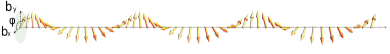
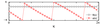
Figure 2: Projected Heisenberg ground state. (Top) Schematic plot showing the helical precession of the Bloch vector parametrizing the projected state, $|\widetilde{\Psi}\rangle=\cos\frac{\theta}{2}|B\rangle+\sin\frac{\theta}{2}e^{i\varphi}|\bar{B}\rangle$. (Bottom) Spherical angles $\varphi$ and $\theta$. Over the cycle $\kappa=0\rightarrow 2\pi$, $\theta$ remains a constant $\frac{\pi}{2}$, and $\varphi(\kappa)$ changes by $-6\pi$, hence the winding number of $\hat{b}$ is $-3$, consistent with a Berry phase of $\pi(\text{mod }2\pi)$. $N=12$ spin-1 sites are used. The ground state is truncated to the many-body basis $|B\rangle=|\uparrow\uparrow\uparrow\uparrow 0\downarrow\downarrow\downarrow\downarrow\uparrow\downarrow 0\rangle$ and its inversion partner.

When $\beta\neq\frac{1}{3}$, the Hamiltonian is no longer a projection operator onto bond singlets, hence there is a proliferation of spin configurations in the ground state that violate the sign-alternating string order, and the winding number of a truncated state, $w_{\widetilde{\Psi}}$, is not restricted to $\pm 1$. Nevertheless, since inversion symmetry is intact, the post-truncation Berry phase remains $\pi$, indicating that $w_{\widetilde{\Psi}}$ is an odd integer. Using the Heisenberg model ($\beta=0$), we have numerically verified that (1) if $|B\rangle$ and $|\bar{B}\rangle$ are string ordered, the winding number remains $\pm 1$; if not, the winding number is an odd integer but not necessarily $\pm 1$, see Fig. 2. (2) If we instead twist the Hamiltonian on the bond between ${\boldsymbol{S}}_{\ell}$ and ${\boldsymbol{S}}_{\ell+1}$, the new winding number $w_{\widetilde{\Psi}}^{(\ell)}$ is related to $w_{\widetilde{\Psi}}$ via a “Gauss law”, $w_{\widetilde{\Psi}}^{(\ell)}-w_{\widetilde{\Psi}}=-2\sum_{n=1}^{\ell}s_{n}^{z}$, suggesting that $s_{n}^{z}=\pm 1$ in a given spin configuration act as charge $\mp 2$ sources of winding numbers. (3) For projections that violate inversion symmetry, the Berry phase is in general not quantized any more. These results are numerically robust even though the typical weight on a many-body basis state is exponentially small ($\sim\frac{1}{\sqrt{3^{N}}}$).

Relation with bulk entanglement

Connection between Hilbert space truncation and topology has previously been studied from the perspective of quantum entanglement Peschel (2003); Cheong and Henley (2004); Li and Haldane (2008); Thomale et al. (2010); Pollmann et al. (2010); Prodan et al. (2010); Hughes et al. (2011); Huang and Arovas (2012). We briefly discuss the relation between entanglement and wavefunction truncation in the context of bulk entanglement Hsieh and Fu (2014); Fukui and Hatsugai (2014); Chiou et al. (2016); Legner and Neupert (2013); Schliemann (2013) due to a sublattice bipartition. Consider a single occupied Bloch band $|\psi_{{\boldsymbol{k}}}\rangle$ with momentum ${\boldsymbol{k}}$. Generalization to multiple occupied bands is straightforward. The Schmidt decomposition of $|\psi_{{\boldsymbol{k}}}\rangle$ into two sublattice groups $A$ and $B$ is

$$|\psi_{{\boldsymbol{k}}}\rangle=\sqrt{f_{{\boldsymbol{k}}}}|\widetilde{\psi}_{A,{\boldsymbol{k}}}\rangle\otimes|\emptyset_{B}\rangle+\sqrt{1-f_{{\boldsymbol{k}}}}|\emptyset_{A}\rangle\otimes|\widetilde{\psi}_{B,{\boldsymbol{k}}}\rangle,$$ (5)

where $|\emptyset_{A(B)}\rangle$ and $|\widetilde{\psi}_{{\boldsymbol{k}},A(B)}\rangle$ are respectively the vacuum and the truncated state in part $A(B)$, $f_{{\boldsymbol{k}}}=\langle\psi_{{\boldsymbol{k}}}|P_{A}|\psi_{{\boldsymbol{k}}}\rangle$. $|\widetilde{\psi}_{{\boldsymbol{k}},A}\rangle$ is thus an entanglement eigenstate for part $A$ in the single particle sector, with entanglement eigenvalue $f_{{\boldsymbol{k}}}$. For a partition with $N_{A}$ sublattices in $A$, there should be a total of $N_{A}$ (single particle) entanglement levels, thus $N_{A}-1$ of them are identically zero. If $f_{{\boldsymbol{k}}}\neq 0\forall{\boldsymbol{k}}$, it is gapped from the remainder, hence one can introduce a topological index, such as an entanglement Chern number Fukui and Hatsugai (2014), for the corresponding entanglement eigenstate, i.e., the truncated state $|\widetilde{\psi}_{{\boldsymbol{k}},A}\rangle$. Truncation invariance thus implies that the entanglement topological index must be identical to the topological index of the parent state if (1) the bulk entanglement spectrum is gapped from zero, and (2) for SPT parent states, the entanglement partition preserves the protecting symmetry.

Measuring topological index via partial tomography

Truncation invariance of the topological index is experimentally relevant. Recent breakthrough in quench-based quantum tomography has made it possible to extract topological indices of two-component Bloch wavefunctions by performing a full measurement of both wavefunction components over the entire BZ (of Bloch momenta) Hauke et al. (2014); Fläschner et al. (2016). We now discuss a quench-based partial quantum tomography for a multi-component Bloch wavefunction $|\psi({\boldsymbol{k}})\rangle=\sum_{a=1}^{N}\psi_{a}({\boldsymbol{k}})|a\rangle$, from which two chosen components $\psi_{a_{1}}({\boldsymbol{k}})$ and $\psi_{a_{2}}({\boldsymbol{k}})$ can be measured. Here $a$ labels sublattices within a unit cell. Combined with truncation invariance, this allows us to determine the Chern number of the full state $|\psi({\boldsymbol{k}})\rangle$. We follow the experimental protocol of Refs. Hauke et al. (2014); Fläschner et al. (2016). Assume at $t=0$ the system has been prepared as a filled Bloch band described by $|\psi({\boldsymbol{k}})\rangle$. For $0<t<t_{h}$, we quench the system with a flat band Hamiltonian $H({\boldsymbol{k}})=\sum_{a=1}^{N}\varepsilon_{a}|a\rangle\langle a|$. The values of $\{\varepsilon_{a}\}$ will be specified later. At the end of the quench, one has $|\psi({\boldsymbol{k}},t_{h})\rangle=\sum_{a=1}^{N}\psi_{a}({\boldsymbol{k}},t_{h})|a\rangle$ where $\psi_{a}({\boldsymbol{k}},t_{h})=\psi_{a}({\boldsymbol{k}})e^{-i\varepsilon_{a}t_{h}}$. The system is then released for a time of flight (TOF) measurement. The resulting momentum distribution from the TOF analysis is given by Hauke et al. (2014) $n({\boldsymbol{k}},t_{h})=\left|\sum_{a=1}^{N}\psi_{a}({\boldsymbol{k}},t_{h})\right|^{2}$, and by monitoring $n({\boldsymbol{k}},t_{h})$ as a continuous function of $t_{h}$, contributions from different $\psi_{a}({\boldsymbol{k}})$ (at $t=0$) can in principle be resolved.

To perform a partial tomography on, say, the first two sublattices $a=1,2$, we set $\varepsilon_{a}$ for all other sublattices $a>2$ to a common level $E$, and require that $\varepsilon_{1}\neq\varepsilon_{2}\neq E$. Consequently, the momentum distribution $n({\boldsymbol{k}},t_{h})$ has only three distinctive frequency modes,

$$\omega_{1(2)}=\varepsilon_{1(2)}-E\ ,\ \omega_{3}=\varepsilon_{2}-\varepsilon_{1}\ ,$$ (6)

and from the TOF experiment, one can extract the corresponding Fourier coefficients $A_{i},B_{i}$,

$$n({\boldsymbol{k}},t_{h})=A_{0}({\boldsymbol{k}})+\sum_{i=1}^{3}\Bigl{[}A_{i}({\boldsymbol{k}})\cos(\omega_{i}t_{h})+B_{i}({\boldsymbol{k}})\sin(\omega_{i}t_{h})\Bigr{]}\ .$$ (7)

Parametrize $\psi_{1}=u\sin\frac{\theta}{2}$ and $\psi_{2}=-u\cos\frac{\theta}{2}e^{i\varphi}$, $u>0$. The overall scale $u$ does not enter the topological index evaluation. The Bloch vector angles $\varphi$ and $\theta$ are

$$\tan\varphi({\boldsymbol{k}})=\frac{B_{3}({\boldsymbol{k}})}{A_{3}({\boldsymbol{k}})}\ ,\ \tan\frac{\theta({\boldsymbol{k}})}{2}=\sqrt{\frac{A_{1}^{2}({\boldsymbol{k}})+B_{1}^{2}({\boldsymbol{k}})}{A_{2}^{2}({\boldsymbol{k}})+B_{2}^{2}({\boldsymbol{k}})}}\ ,$$ (8)

see SM for derivation and $\varphi$,$\theta$ plots of a truncated Hofstadter band. Eq. 8 allows us to extract the projected state $|\widetilde{\psi}\rangle=(\frac{\psi_{1}}{u},\frac{\psi_{2}}{u})^{t}$, from which the Chern number of the full state can be computed. In fact, since $|\widetilde{\psi}\rangle$ is also a bulk entanglement eigenstate, this is a measurement protocol for the entanglement Chern number of a sublattice truncation as discussed in the previous section.

Conclusion

We have shown that a normalizable truncated wavefunction preserves the topological index of its parent state, if both indices are computed in the space of the parent state’s twisted boundary phases. The physical interpretation of the index may change for the truncated state if its boundary condition is affected by the truncation, and we gave an example using the parton construction of the $\textsf{SU}(m)$ FCI state. We also showed that a sublattice-truncated state can be identified as an entanglement eigenstate resulting from a sublattice bipartition, revealing a connection between wavefunction truncation and quantum entanglement. Our finding provides a new perspective on the topological structure of wavefunctions, and indicates that mathematical specification of a topological index, and perhaps even its physical manifestation, can be achieved in a much smaller Hilbert space, such as the 2-sublattice space that may be probed by the partial tomography scheme discussed in the text.

Acknowledgments

We are grateful to Yi Zhang for critical reading and comments of an early draft, and to D. N. Sheng, Kai Sun, Christof Weitenberg, Avadh Saxena, Hongchul Choi, and S. Kourtis for useful discussions and communications. W.Z. thanks T. S. Zeng for helpful discussion and F. D. M. Haldane for education of the physics of spin-1 antiferromagnetic chain. Work at LANL was supported by US DOE BES E3B7 (ZSH, JXZ, and AVB), and by US DOE NNSA through LANL LDRD (ZSH, WZ, and AVB). Work at NORDITA was supported by ERC DM 321031 (AVB).

I Supplemental Materials

In this note, we give additional examples and derivations showing truncation invariance in (1) the Hofstadter model, a band Chern insulator, (2) the BHZ model, a time-reversal-invariant $Z_{2}$ topological insulator, (3) the AKLT model, which belongs to the $Z_{2}$ Haldane phase and (4) a fractional Chern insulator model hosting non-Abelian fractional quantum Hall effect. We also provide derivation details of the partial quantum tomography scheme introduced in the main text, and discuss the relation and distinction of truncation invariance with recent works on the node structure in wavefunction overlaps.

II Hofstadter model

We go through the general proof of truncation invariance of the Chern number in detail, and and provide additional demonstrations, using the paradigmatic Hofstadter model Hofstadter (1976). This model describes electrons hopping on a square lattice in the $xy$ plane placed in a uniform magnetic field along $z$. For a rational flux per square plaquette, $\phi=2\pi p/q$ ($p$ and $q$ are coprime integers), the magnetic unit cell consists of $q$ consecutive plaquettes, which we choose to align in the $y$ direction. Correspondingly, there are $q$ Bloch bands. Each band wavefunction can be expressed as a $q$-element column vector, $|\psi({\boldsymbol{k}})\rangle=(\psi_{1}({\boldsymbol{k}}),\psi_{2}({\boldsymbol{k}}),\cdots,\psi_{q}({\boldsymbol{k}}))^{t}$, where $\psi_{a}({\boldsymbol{k}})=\langle a|\psi({\boldsymbol{k}})\rangle$ and $|a\rangle$ is the atomic state on the $a^{th}$ site of the magnetic unit cell.

II.1 Wavefunction zeros and phase vortices

In this section, we go through the general proof of truncation invariance of the Chern number in more detail, using the three-band case $p/q=1/3$ as an example. The lowest band $|\psi({\boldsymbol{k}})\rangle$ has a Chern number $C=1$, therefore all three of its wavefunction components, $\psi_{i}({\boldsymbol{k}}),i=1,2,3$, have at least one zero in the Brillouin zone. One can verify that the zeros of $\psi_{1},\psi_{2}$, and $\psi_{3}$ occur at $k_{y}=0$ and $k_{x}=\frac{4\pi}{3},\frac{2\pi}{3}$, and $0$, respectively, see Fig. 3.

To compute the Chern number of $|\psi({\boldsymbol{k}})\rangle$, we now divide the Brillouin zone into two patches, see Fig. 4. One patch, denoted as $R_{2}$, is an infinitesimal neighborhood of radius $\epsilon$ around the zero of $\psi_{1}$, at ${\boldsymbol{k}}_{1}=(\frac{4\pi}{3},0)$: $R_{2}=\{{\boldsymbol{k}}:|{\boldsymbol{k}}-{\boldsymbol{k}}_{1}|\leq\epsilon\}$. The remainder constitutes the other patch, $R_{1}=\{{\boldsymbol{k}}:|{\boldsymbol{k}}-{\boldsymbol{k}}_{1}|\geq\epsilon\}$. Since $\psi_{1}$ has only one zero at ${\boldsymbol{k}}_{1}$, one can always choose a gauge for $R_{1}$ such that $\psi_{1}$ is real and positive,

$$|\psi({\boldsymbol{k}})\rangle_{R_{1}}=\begin{pmatrix}|\psi_{1}({\boldsymbol{k}})|\\ |\psi_{2}({\boldsymbol{k}})|e^{i\phi_{2}({\boldsymbol{k}})}\\ |\psi_{3}({\boldsymbol{k}})|e^{i\phi_{3}({\boldsymbol{k}})}\end{pmatrix}\quad,\quad{\boldsymbol{k}}\in R_{1}\ .$$ (9)

We have used the subscript $R_{1}$ to denote the gauge choice. In the patch $R_{2}$, we instead choose a gauge where $\psi_{2}$ is real and positive. This is always achievable because the zeros of $\psi_{1}$ and $\psi_{2}$ do not coincide, see Fig. 3. Thus

$$|\psi({\boldsymbol{k}})\rangle_{R_{2}}=\begin{pmatrix}|\psi_{1}({\boldsymbol{k}})|e^{i\varphi_{1}({\boldsymbol{k}})}\\ |\psi_{2}({\boldsymbol{k}})|\\ |\psi_{3}({\boldsymbol{k}})|e^{i\varphi_{3}({\boldsymbol{k}})}\end{pmatrix}\quad,\quad{\boldsymbol{k}}\in R_{2}\ .$$ (10)

On the interface between the two patches, defined as

$$R_{1}\cap R_{2}=\{{\boldsymbol{k}}_{\cap}:|{\boldsymbol{k}}-{\boldsymbol{k}}_{1}|=\epsilon\}\ ,$$ (11)

$|\psi({\boldsymbol{k}})\rangle_{R_{1}}$ and $|\psi({\boldsymbol{k}})\rangle_{R_{2}}$ differ by an overall phase $\lambda({\boldsymbol{k}})$,

$$|\psi({\boldsymbol{k}}_{\cap})\rangle_{R_{1}}=e^{i\lambda({\boldsymbol{k}}_{\cap})}|\psi({\boldsymbol{k}}_{\cap})\rangle_{R_{2}}\quad,\quad{\boldsymbol{k}}_{\cap}\in R_{1}\cap R_{2}\ .$$ (12)

From Eqs. 9 and 10, one has that

$$\lambda({\boldsymbol{k}}_{\cap}) =-\varphi_{1}({\boldsymbol{k}}_{\cap})=\phi_{2}({\boldsymbol{k}}_{\cap})$$

$$=\textsf{Arg}\frac{\psi_{2}({\boldsymbol{k}}_{\cap})}{\psi_{1}({\boldsymbol{k}}_{\cap})}\quad,\quad{\boldsymbol{k}}_{\cap}\in R_{1}\cap R_{2}\ .$$ (13)

The second line is manifestly gauge invariant.

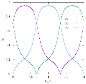
Figure 3: The lowest subband wavefunction of the $p/q=1/3$ Hofstadter model, at $k_{y}=0$. All three components show one zero as $k_{x}$ varies from $0$ to $2\pi$, consistent with the band Chern number being $C=1$. We have verified that the zeros only occur at $k_{y}=0$.

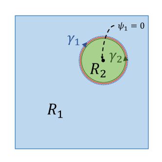
Figure 4: Schematics of the wavefunction gauge choice according to the zero of $\psi_{1}({\boldsymbol{k}})$. The Chern number computed with this gauge is the sum of two Berry phases, $\gamma_{1}$ along $\partial R_{1}$ in clockwise direction, and $\gamma_{2}$ along $\partial R_{2}$ in counter-clockwise direction.

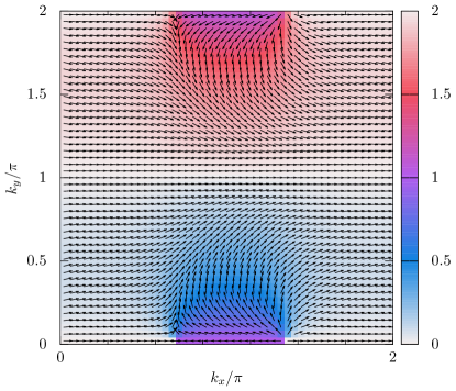
(a) $\textsf{Arg}\frac{\psi_{2}}{\psi_{1}}$

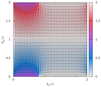
(b) $\textsf{Arg}\frac{\psi_{3}}{\psi_{2}}$

Figure 5: Phases of $\psi_{2}/\psi_{1}$ and $\psi_{3}/\psi_{2}$ for the lowest band of the $p/q=1/3$ Hofstadter model. Color encodes the phase angles in unit of $\pi$, and arrows show the same information represented as polar vectors $(\cos\varphi_{{\boldsymbol{k}}},\sin\varphi_{{\boldsymbol{k}}})$. The phases show two singularities corresponding to the zero of the numerator and the denominator, respectively. The zero of the denominator is a vortex of the relative phase, around which the relative phase has a winding number $1$. The zero of the numerator is an anti-vortex of the relative phase, around which the relative phase has a winding number $-1$; see Fig. 3 for the location of zeros. Following the general construction outlined in the text, the Chern number of both the truncated state and the untruncated state can be identified as the winding number of the phase around the zero of the denominator, and equivalently the negative winding number of around the zero of the numerator.

The Chern number of $|\psi({\boldsymbol{k}})\rangle$ can now be computed as

$$C=\frac{1}{2\pi}\iint\limits_{BZ}d^{2}k\nabla_{{\boldsymbol{k}}}\times\langle\psi({\boldsymbol{k}})|i\nabla_{{\boldsymbol{k}}}|\psi({\boldsymbol{k}})\rangle=\frac{1}{2\pi}(\iint\limits_{R_{1}}+\iint\limits_{R_{2}})\cdots=\frac{1}{2\pi}\sum_{i=1,2}\oint\limits_{\partial R_{i}}d{\boldsymbol{k}}_{\cap}\cdot\langle\psi({\boldsymbol{k}}_{\cap})|i\nabla_{{\boldsymbol{k}}_{\cap}}|\psi({\boldsymbol{k}}_{\cap})\rangle_{R_{i}}\ ,$$ (14)

where we have used Stokes theorem to convert the area integrals over $R_{1}$ and $R_{2}$ into line integrals over their boundaries. Note that the two boundaries, $\partial R_{1}$ and $\partial R_{2}$, are identical but in opposite directions; both consist of the infinitesimal loop Eq. 11, with $\partial R_{2}$ in the counter-clockwise and $\partial R_{1}$ in the clockwise direction. The Chern number is thus

$$C=\frac{1}{2\pi}\ointctrclockwise\limits_{R_{1}\cap R_{2}}d{\boldsymbol{k}}_{\cap}\cdot\Bigl{[}\langle\psi({\boldsymbol{k}}_{\cap})|i\nabla_{{\boldsymbol{k}}_{\cap}}|\psi({\boldsymbol{k}}_{\cap})\rangle_{R_{2}}-\langle\psi({\boldsymbol{k}}_{\cap})|i\nabla_{{\boldsymbol{k}}_{\cap}}|\psi({\boldsymbol{k}}_{\cap})\rangle_{R_{1}}\Bigr{]}=\frac{1}{2\pi}\ointctrclockwise\limits_{R_{1}\cap R_{2}}d{\boldsymbol{k}}_{\cap}\cdot\nabla_{{\boldsymbol{k}}_{\cap}}\lambda({\boldsymbol{k}}_{\cap})\equiv w[\lambda]\ ,$$ (15)

which is the counter-clockwise winding number of the gauge invariant phase mismatch $\lambda({\boldsymbol{k}}_{\cap})$. To obtain the second equality, we have used $\langle e^{-i\lambda({\boldsymbol{k}})}\psi({\boldsymbol{k}})|i\nabla_{{\boldsymbol{k}}}|e^{i\lambda({\boldsymbol{k}})}\psi({\boldsymbol{k}})\rangle=\langle\psi({\boldsymbol{k}})|i\nabla_{{\boldsymbol{k}}}|\psi({\boldsymbol{k}})\rangle-\nabla_{{\boldsymbol{k}}}\lambda({\boldsymbol{k}})$. This is also equivalent to the difference of Berry phases evaluated with the two different gauges $|\psi\rangle_{R_{1}}$ and $|\psi\rangle_{R_{2}}$, over the same path $R_{1}\cap R_{2}$ in counter-clockwise direction, see Fig. 4. It is known that when evaluated with different gauge choices, the physical (gauge invariant) Berry phase is only defined up to integer multiples $2\pi$, and we see that the said integer, in this context, is the Chern number.

The above computational scheme for the Chern number can be summarized as: The Chern number of $|\psi({\boldsymbol{k}})\rangle$ can be computed from any two components, $\psi_{i_{1}}$ and $\psi_{i_{2}}$, as the winding number of the gauge invariant relative phase $\textsf{Arg}\frac{\psi_{i_{2}}}{\psi_{i_{1}}}$ around the zero of the denominator $\psi_{i_{1}}$. If multiple zeros exist, the Chern number is the total vorticity around these zeros.

Since truncation does not change the ratio between any pair of wavefunction elements, the Chern number of a renormalizable truncated state must be the same as the parent state.

II.2 Sublattice truncation invariance

We consider truncation to a $2$-sublattice Hilbert space, $|\widetilde{\psi}({\boldsymbol{k}})\rangle\equiv(\widetilde{\psi}_{i_{1}}({\boldsymbol{k}}),\widetilde{\psi}_{i_{2}}({\boldsymbol{k}}))^{t}$, where $\widetilde{\psi}_{i_{1}}/\widetilde{\psi}_{i_{2}}=\psi_{i_{1}}/\psi_{i_{2}}$ and $\langle\widetilde{\psi}|\widetilde{\psi}\rangle=1$. $|\widetilde{\psi}({\boldsymbol{k}})\rangle$ can be parametrized by a vector $\hat{b}\equiv(\theta,\varphi)$ on the unit Bloch sphere, $\widetilde{\psi}_{i_{1}}=\sin\frac{\theta}{2}$ and $\widetilde{\psi}_{i_{2}}=-\cos\frac{\theta}{2}e^{i\varphi}$. This parametrization is also used in the partial tomography discussed in the text and a later section in this SM. The Chern number of $\widetilde{\psi}$ measures the number of times $\hat{b}$ covers the Bloch sphere, $\widetilde{C}=\frac{1}{4\pi}\iint d^{2}k\ \hat{b}({\boldsymbol{k}})\cdot\Bigl{[}\partial_{k_{x}}\hat{b}({\boldsymbol{k}})\times\partial_{k_{y}}\hat{b}({\boldsymbol{k}})\Bigr{]}$. In Fig. 6, we plot the Bloch vector $\hat{b}({\boldsymbol{k}})$ for the state truncated to sublattices $(i_{1},i_{2})=(1,2)$. The parent state is chosen as the lowest Hofstadter band with flux $p/q=3/7$, which has a Chern number of $C=-2$. One can verify from Fig. 6 that $\widetilde{C}=C$.

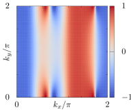
(a) $\cos\theta({\boldsymbol{k}})$

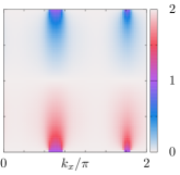
(b) $\varphi({\boldsymbol{k}})/\pi$

Figure 6: Bloch vector representation of a $2$-element truncation of a Hofstadter band. We truncate the lowest band $|\psi({\boldsymbol{k}})\rangle$ to sublattices $1$ and $2$, $P|\psi\rangle/\sqrt{\langle\psi|P|\psi\rangle}=(\widetilde{\psi}_{1},\widetilde{\psi}_{2})^{t}\equiv(\sin\frac{\theta}{2},-\cos\frac{\theta}{2}e^{i\varphi})$. The Hofstadter flux is set as $p/q=3/7$, hence $|\psi({\boldsymbol{k}})\rangle$ has a Chern number $C=-2$. Panel (a): $z$-component of the Bloch vector, $b_{z}=\cos\theta$. Panel (b): its azimuthal angle $\varphi$. The north pole of the Bloch sphere ($b_{z}=1$) can be identified as the darkest red spots in (a), and the south pole ($b_{z}=-1$) the darkest blue spots, all located on $k_{y}=0$. Each pole is covered twice, consistent with $C=-2$. The azimuth $\varphi$ around each pole exhibits a vortex ($\varphi$ traverses $0\rightarrow 2\pi$ going around a pole), as can be verified in (b). Vertical white stripes in (a) correspond to the equator of the Bloch sphere ($b_{z}=0$); of the four such stripes, only two have $\varphi$ winding from $0$ to $2\pi$ in (b), hence the equator is also covered twice, consistent with $C=-2$.

III BHZ model

We use the BHZ model to illustrate truncation invariance of the $Z_{2}$ class in 2D, which, in principle, follows from the invariance of the spin Chern number. The BHZ model has a four-element unit cell $(A_{\uparrow},B_{\uparrow},A_{\downarrow},B_{\downarrow})$, where $A,B$ denote sublattices and $\uparrow,\downarrow$ denote spin. The Hamiltonian is Bernevig et al. (2006)

$$H({\boldsymbol{k}})=\sin k_{x}\sigma_{z}\otimes\tau_{x}+\sin k_{y}\mathbb{I}\otimes\tau_{y}+(2-m-\cos k_{x}-\cos k_{y})\mathbb{I}\otimes\tau_{z}+\Delta\sigma_{y}\otimes\tau_{y}\ ,$$ (16)

where $\tau$ and $\sigma$ are Pauli matrices acting on the sublattice and spin spaces, respectively, and $\Delta\neq 0$ breaks inversion symmetry.

We will implement a truncation by projecting out every other $A$ site along the $x$ direction for both spin species. This effectively doubles the unit cell along $x$, yielding an $8$-band model prior to truncation. The Hamiltonian with doubled unit cell is

$$H(q_{x},k_{y})=\begin{pmatrix}H_{0}&H_{1}+H_{-1}e^{-iq_{x}}\\ H_{-1}+H_{1}e^{iq_{x}}&H_{0}\end{pmatrix}\ ,$$ (17)

where $q_{x}$ is the Bloch momentum with respect to the doubled unit cell along $x$, and the $k_{y}$-dependent $4\times 4$ blocks are

$$H_{0}(k_{y})=\sin k_{y}\mathbb{I}\otimes\tau_{y}+(2-m-\cos k_{y})\mathbb{I}\otimes\tau_{z}+\Delta\sigma_{y}\otimes\tau_{y}\ ,$$ (18)

$$H_{\pm 1}(k_{y})=\pm\frac{1}{2i}\sigma_{z}\otimes\tau_{x}-\frac{1}{2}\mathbb{I}\otimes\tau_{z}\ .$$ (19)

In Fig. 7, we compare the Wannier spectral flow Yu et al. (2011) of the ground state at half filling (black dots) with that of a truncated state (purple circles). The $Z_{2}$ index can be identified Yu et al. (2011) as the parity of the number of times the Wannier spectra cross a given value of Wannier center (a constant $\gamma$ in Fig. 7) in the half BZ $k_{x}\in[0,\pi]$. The truncated state preserves time reversal symmetry because $A_{\uparrow}$ and $A_{\downarrow}$ are time reversal partners, hence it still allows for a $Z_{2}$ classification. Fig. 7 shows that the $Z_{2}$ index is indeed truncation invariant.

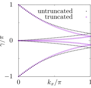
(a) $Z_{2}=1$

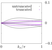
(b) $Z_{2}=0$

Figure 7: Wannier spectral flow of the full and truncated BHZ ground state (at half filling), demonstrating that a symmetry-preserving truncation does not change the $Z_{2}$ index. The BHZ model has two sublattices $A$ and $B$, and we use a truncation where every other $A$ sublattice along the $x$ direction is projected out. This breaks the invariance of translation by one unit cell along the $x$ direction, and effectively doubles the unit cell size, hence there are four Wannier spectral lines (instead of two). Black dots: Wannier flow of the untruncated state. Purple circles: Wannier flow of the truncated state. (a): Non-trivial phase (parameters: $\Delta=0.3,m=1.1$). (b): Trivial phase ($\Delta=0.3,m=-1.1$). Note different $y$-scales.

IV Berry phase of truncated $S=1$ AKLT wavefunctions

The $S=1$ AKLT wavefunction of $N$ spins with a twisted boundary phase $\kappa$ is

$$|\Psi(\kappa)\rangle=(a_{N}^{\dagger}b_{1}^{\dagger}e^{i\kappa}-b_{N}^{\dagger}a_{1}^{\dagger})\prod_{i=1}^{N-1}(a_{i}^{\dagger}b_{i+1}^{\dagger}-b_{i}^{\dagger}a_{i+1}^{\dagger})|\emptyset\rangle\ ,$$ (20)

where $a$ and $b$ are Schwinger bosons satisfying

$$S_{i}^{+}=a_{i}^{\dagger}b_{i}\quad,\quad S_{i}^{z}=\frac{1}{2}(a_{i}^{\dagger}a_{i}-b_{i}^{\dagger}b_{i})\quad,\quad a_{i}^{\dagger}a_{i}+b_{i}^{\dagger}b_{i}\stackrel{{\scriptstyle!}}{{=}}2\ ,$$ (21)

and $|\emptyset\rangle$ is the boson vacuum. On the $i^{th}$ site, one has

$$(a_{i}^{\dagger})^{2}|\emptyset\rangle=\sqrt{2}|\uparrow\rangle\quad,\quad a_{i}^{\dagger}b_{i}^{\dagger}|\emptyset\rangle=|0\rangle\quad,\quad(b_{i}^{\dagger})^{2}|\emptyset\rangle=\sqrt{2}|\downarrow\rangle\ .$$ (22)

Inversion $\mathcal{I}$ is defined as

$$\mathcal{I}a_{i}\mathcal{I}^{-1}=a_{N+1-i}\quad,\quad\mathcal{I}b_{i}\mathcal{I}^{-1}=b_{N+1-i}\quad,\quad\mathcal{I}i\mathcal{I}^{-1}=i\ .$$ (23)

This implies that $|\Psi(\kappa)\rangle$ transforms under inversion as

$$\mathcal{I}|\Psi(\kappa)\rangle=(-1)^{N}e^{i\kappa}|\Psi(-\kappa)\rangle\ .$$ (24)

When fully expanded, Eq. 20 contains $2^{N}$ monomials by selecting one of the two terms $\{a_{i}^{\dagger}b_{i+1}^{\dagger},b_{i}^{\dagger}a_{i+1}^{\dagger}\}$ from each bond . One can verify the spin configurations corresponding to the monomials in the resulting expansion must satisfy a string order, wherein the nonzero spins have alternating signs. For example, $|1,0,\cdots,0,-1\rangle\propto a_{1}^{\dagger}b_{2}^{\dagger}\cdot a_{2}^{\dagger}b_{3}^{\dagger}\cdots a_{N-1}^{\dagger}b_{N}^{\dagger}\cdot b_{N}^{\dagger}a_{1}^{\dagger}|\emptyset\rangle$, and the (ordered) list of its nonzero spins $\{1,-1\}$ satisfies the string order.

To gain intuition on the form of projected wavefunctions, consider first the projection onto a spin configuration $|B_{0}\rangle$ and its inversion conjugate $|\bar{B}_{0}\rangle$, where

$$|B_{0}\rangle=|1,0,0,\cdots,0,0,-1\rangle\quad,\quad|\bar{B}_{0}\rangle=\mathcal{I}|B_{0}\rangle=|-1,0,0,\cdots,0,0,1\rangle\ .$$ (25)

There is only one monomial in the expansion of Eq. 20 that has non-zero overlap with $|B_{0}\rangle$,

$$\langle B_{0}|\Psi(\kappa)\rangle=\langle B_{0}|a_{1}^{\dagger}b_{2}^{\dagger}\cdot a_{2}^{\dagger}b_{3}^{\dagger}\cdots\cdot a_{N-1}^{\dagger}b_{N}^{\dagger}\cdot(-b_{N}^{\dagger}a_{1}^{\dagger})|\emptyset\rangle=-2\ ,$$ (26)

and similarly for $|\bar{B}_{0}\rangle$,

$$\langle\bar{B}_{0}|\Psi(\kappa)\rangle=\langle B_{0}|(-b_{1}^{\dagger}a_{2}^{\dagger})\cdot(-b_{2}^{\dagger}a_{3}^{\dagger})\cdots\cdot(-b_{N-1}^{\dagger}a_{N}^{\dagger})\cdot(a_{N}^{\dagger}b_{1}^{\dagger}e^{i\kappa}|\emptyset\rangle=(-1)^{N-1}\times 2e^{i\kappa}\ ,$$ (27)

which can be alternatively obtained as $\langle B_{0}|\mathcal{I}\Psi(\kappa)\rangle$. The resulting normalized projected wavefunction is thus

$$|\widetilde{\Psi}(\kappa)\rangle_{B_{0}}=\frac{1}{\sqrt{2}}\left(|B_{0}\rangle+(-1)^{N}e^{i\kappa}|\bar{B}_{0}\rangle\right)\ .$$ (28)

The factor $(-1)^{N}$ arises due to the inversion conjugacy between $|B_{0}\rangle$ and $|\bar{B}_{0}\rangle$.

One observes from the above example that the phase in the wavefunction coefficient of $|B_{0}\rangle$ depends only on which term in the boundary link, $a_{N}^{\dagger}b_{1}^{\dagger}e^{i\kappa}$ or $-b_{N}^{\dagger}a_{1}^{\dagger}$, is present in the monomial. If the leftmost nonzero spin in a configuration $|B_{0}\rangle$ is $1$, then string order demands that $-b_{N}^{\dagger}a_{1}^{\dagger}$ be present, and the corresponding wavefunction coefficient is purely real, whereas if it is $-1$, $a_{N}^{\dagger}b_{1}^{\dagger}e^{i\kappa}$ will be present, and the corresponding wavefunction coefficient has a phase $e^{i\kappa}$. This observation is in fact true for any string ordered configuration $|B\rangle$, and the projected state is

$$|\widetilde{\Psi}(\kappa)\rangle_{B}=\frac{1}{\sqrt{2}}\left(|B\rangle+(-1)^{N}e^{is\kappa}|\bar{B}\rangle\right)\ ,$$ (29)

where $s$ is the leftmost nonzero spin in configuration $B$.

V Quench protocol for partial tomography

In a time-of-flight measurement of a Fermi gas released from an optical lattice, the momentum distribution is Bloch et al. (2008)

$$n({\boldsymbol{k}})\propto|\widetilde{w}({\boldsymbol{k}})|^{2}\mathcal{G}({\boldsymbol{k}})\ ,$$ (30)

where $\widetilde{w}({\boldsymbol{k}})$ is the Fourier transform of Wannier functions and $\mathcal{G}({\boldsymbol{k}})$ is the Fourier transform of the one-particle correlation matrix at the time of release, $\mathcal{G}({\boldsymbol{k}})=\sum_{{\boldsymbol{R}},{\boldsymbol{R}}^{\prime}}e^{i{\boldsymbol{k}}\cdot({\boldsymbol{R}}-{\boldsymbol{R}}^{\prime})}\langle c^{\dagger}_{{\boldsymbol{R}}}c^{\phantom{}}_{{\boldsymbol{R}}^{\prime}}\rangle$. Here, $c^{\dagger}_{{\boldsymbol{R}}}$ is the creation operator at lattice site ${\boldsymbol{R}}$. If there is a sublattice structure, ${\boldsymbol{R}}$ becomes a composite label, ${\boldsymbol{R}}={\boldsymbol{X}}+{\boldsymbol{r}}_{a}$, where ${\boldsymbol{X}}$ is the spatial coordinate associated with the center of a unit cell, and ${\boldsymbol{r}}_{a}$ is the position of the $a^{th}$ sublattice within a unit cell. Using the Fourier transform $c_{{\boldsymbol{k}},a}^{\dagger}=e^{i{\boldsymbol{k}}\cdot{\boldsymbol{r}}_{a}}\left[\sum_{{\boldsymbol{X}}}e^{i{\boldsymbol{k}}\cdot{\boldsymbol{X}}}c_{{\boldsymbol{X}},a}^{\dagger}\right]$, the correlation matrix becomes $\mathcal{G}({\boldsymbol{k}})=\sum_{a,b}\langle c_{{\boldsymbol{k}},a}^{\dagger}c_{{\boldsymbol{k}},b}^{\phantom{}}\rangle$. The correlator is evaluated with the many-body state $|\Psi\rangle$ of the Fermi gas at the time of release. For a filled Bloch band, $|\Psi\rangle=\prod_{{\boldsymbol{q}}\in BZ}\psi_{{\boldsymbol{q}}}^{\dagger}|\emptyset\rangle$, where $\psi_{{\boldsymbol{q}}}^{\dagger}$ creates a Bloch band state of momentum ${\boldsymbol{q}}$: $\langle\emptyset|c_{{\boldsymbol{X}},a}\psi_{{\boldsymbol{q}}}^{\dagger}|\emptyset\rangle\equiv e^{i{\boldsymbol{q}}\cdot({\boldsymbol{X}}+{\boldsymbol{r}}_{a})}\psi_{a}({\boldsymbol{q}})$, and $\psi_{a}({\boldsymbol{q}})$ is the Bloch cell function on sublattice $a$. Knowledge of $\psi_{a}({\boldsymbol{q}})$ for all ${\boldsymbol{q}}$ and $a$ would allow the calculation of the topological index of the single particle Bloch band $|\psi({\boldsymbol{q}})\rangle=(\psi_{1}({\boldsymbol{q}}),\psi_{2}({\boldsymbol{q}}),\cdots,\psi_{N_{B}}({\boldsymbol{q}}))^{t}$, where $N_{B}$ is the number of sublattices within a unit cell. Using Wick’s theorem, one then has

$$\mathcal{G}({\boldsymbol{k}})=\sum_{a,b}\langle\emptyset|\psi_{{\boldsymbol{k}}}^{\phantom{}}c_{{\boldsymbol{k}},a}^{\dagger}c_{{\boldsymbol{k}},b}^{\phantom{}}\psi_{{\boldsymbol{k}}}^{\dagger}|\emptyset\rangle=\left|\sum_{a}\psi_{a}({\boldsymbol{k}})\right|^{2}\ .$$ (31)

Following Ref. Hauke et al., 2014, we will ignore the Wannier envelope $\widetilde{w}({\boldsymbol{k}})$ in the momentum distribution, and treat the correlator $\mathcal{G}({\boldsymbol{k}})$ itself as the momentum distribution. This is justified because in the quench protocal to be discussed below, $\widetilde{w}({\boldsymbol{k}})$ does not pick up a time dependence, and since everything of interest will turn out to depend on a ratio, the $\widetilde{w}({\boldsymbol{k}})$ dependence will drop out. Here we also assume that all atomic basis states originate from the same orbital, e.g., the $s$ orbital. If basis states arise from different orbitals, their Wannier envelopes will not cancel each other in the way described above Weitenberg .

From Eq. 31, different wavefunction components (labeled by $a$) are intermixed in the momentum distribution and thus cannot be distinguished from each other. The key insight of Refs. Hauke et al., 2014; Fläschner et al., 2016 is that they can be separated in time domain if the state $|\Psi\rangle$ is subjected to a quench, for a duration $t_{h}$ before the ToF measurement, by a flat band Hamiltonian $H_{\text{FB}}=\sum_{{\boldsymbol{k}},a}\varepsilon_{a}c_{{\boldsymbol{k}},a}^{\dagger}c_{{\boldsymbol{k}},a}^{\phantom{}}$ between $0<t<t_{h}$. $H_{\text{FB}}$ can be achieved by “turning off” electron hopping, and bias different sublattices at different potentials $\varepsilon_{a}$. As a consequence, each wavefunction component will pick up a distinctive dynamical phase at the end of the quench, $\psi_{a}({\boldsymbol{k}},t_{h})=\psi_{a}({\boldsymbol{k}})e^{-i\varepsilon_{a}t_{h}}$. The electrons are then released for a time-of-flight measurement. The resulting momentum distribution is thus

$$n({\boldsymbol{k}},t_{h})=\left|\sum_{a}\psi_{a}({\boldsymbol{k}})e^{-i\varepsilon_{a}t_{h}}\right|^{2}\ ,$$ (32)

note that we have dropped the $\widetilde{w}({\boldsymbol{k}})$ dependence as discussed before, and rescaled to a dimensionless $n({\boldsymbol{k}},t_{h})$, see also the Supplementary Material of Ref. Hauke et al., 2014.

In general, $n({\boldsymbol{k}},t_{h})$ will contain terms oscillating at frequencies $\omega_{a,b}=|\varepsilon_{a}-\varepsilon_{b}|$ due to the interference between different sublattices. For $N_{B}$ sublattices, there are $N_{\omega}=N_{B}(N_{B}-1)/2$ such frequencies (assuming no degeneracy in $\omega$), hence there are $2N_{\omega}+1$ real Fourier coefficients $A_{\omega},B_{\omega}$: $n({\boldsymbol{k}},t_{h})=A_{0}({\boldsymbol{k}})+\sum_{\omega}[A_{\omega}({\boldsymbol{k}})\cos(\omega t_{h})+B_{\omega}({\boldsymbol{k}})\sin(\omega t_{h})]$. For a full tomography of $|\psi({\boldsymbol{k}})\rangle$, one needs to deduce $2N_{B}-1$ real-valued unknowns—corresponding to the real and imaginary parts of the $N_{B}$ wavefunction components sans the normalization constraint—from the $2N_{\omega}+1$ experimentally accessible Fourier coefficients. It is easy to check that $2N_{\omega}+1\geq 2N_{B}-1$, for $N_{B}\geq 2$, where equality occurs for $N_{B}=2$. That is, we always have enough Fourier coefficients to fully determine all wavefunction components, hence a full tomography of a band wavefunction is in principle always achievable for any number of sublattices. That we have more than enough Fourier coefficients simply means some of them are not independent. In practice, however, analytical determination of all wavefunction components becomes untractable with increasing $N_{B}$. As shown in the text, such a full tomography is also unnecessary for determining the topological index of a wavefunction, for which a partial tomography of a small subset of wavefunction components would be sufficient. Below, we discuss a quench protocol for partial tomography of two wavefunction components. Note that a full tomography can also be built up from successive partial tomographies.

To perform a partial tomography on, say, the first two sublattices $a=1,2$, we set the flat band energy of all other sublattices to a common level, $\varepsilon_{a>2}=E$, and require that $\varepsilon_{1}\neq\varepsilon_{2}\neq E$. The momentum distribution becomes

$$n({\boldsymbol{k}},t_{h})=\left|\psi_{1}({\boldsymbol{k}})e^{-i\varepsilon_{1}t_{h}}+\psi_{2}({\boldsymbol{k}})e^{-i\varepsilon_{2}t_{h}}+\left(\sum_{a=3}^{N_{B}}\psi_{a}({\boldsymbol{k}})\right)e^{-iEt_{h}}\right|^{2}\ .$$ (33)

Introduce the following parametrization,

$$\psi_{1}({\boldsymbol{k}})=u({\boldsymbol{k}})\sin\frac{\theta({\boldsymbol{k}})}{2}\quad,\quad\psi_{2}({\boldsymbol{k}})=-u({\boldsymbol{k}})\cos\frac{\theta({\boldsymbol{k}})}{2}e^{i\varphi({\boldsymbol{k}})}\quad,\quad\sum_{a=3}^{N_{B}}\psi_{a}({\boldsymbol{k}})=v({\boldsymbol{k}})e^{i\chi({\boldsymbol{k}})}\ ,$$ (34)

where $u({\boldsymbol{k}})>0$, $v({\boldsymbol{k}})\geq 0$, $\theta({\boldsymbol{k}})\in[0,\pi]$, and $\varphi({\boldsymbol{k}}),\chi({\boldsymbol{k}})\in[0,2\pi]$. Further introduce three frequencies,

$$\omega_{1}=\varepsilon_{1}-E\quad,\quad\omega_{2}=\varepsilon_{2}-E\quad,\quad\omega_{3}=\varepsilon_{2}-\varepsilon_{1}\ .$$ (35)

Then $n({\boldsymbol{k}},t_{h})$ has the following Fourier decomposition (suppressing the ${\boldsymbol{k}}$ dependence),

$$n(t_{h})=A_{0}+\sum_{i=1}^{3}\left[A_{i}\cos(\omega_{i}t_{h})+B_{i}\sin(\omega_{i}t_{h})\right]\ ,$$ (36)

$$A_{0}=u^{2}+v^{2}\ ,$$ (37)

$$A_{1}=2uv\sin\frac{\theta}{2}\cos\chi\quad,\quad B_{1}=-2uv\sin\frac{\theta}{2}\sin\chi\ ,$$ (38)

$$A_{2}=-2uv\cos\frac{\theta}{2}\cos(\varphi-\chi)\quad,\quad B_{2}=-2uv\cos\frac{\theta}{2}\sin(\varphi-\chi)\ ,$$ (39)

$$A_{3}=-u^{2}\sin\theta\cos\varphi\quad,\quad B_{3}=-u^{2}\sin\theta\sin\varphi\ .$$ (40)

Note that if $v=0$, $A_{1,2}=B_{1,2}=0$ and we recover the $2$-component formalism of Ref. Hauke et al., 2014. In general, $v\neq 0$, and the Bloch sphere angles $\theta$ and $\varphi$ can be determined as

$$\tan\varphi=\frac{B_{3}}{A_{3}}\quad,\quad\tan\frac{\theta}{2}=\sqrt{\frac{A_{1}^{2}+B_{1}^{2}}{A_{2}^{2}+B_{2}^{2}}}\ .$$ (41)

The overall scale $u$ can be obtained as $u=\sqrt[4]{(A_{3}^{2}+B_{3}^{2})/\sin^{2}\theta}$, although it does not enter the evaluation of topological indices such as the Chern number or the Berry phase. Note that (1) $\varphi$ and $\theta$ only depend on ratios of the Fourier coefficients, and remain unchanged even when the Wannier envelope $\widetilde{w}({\boldsymbol{k}})$ (cf. Eq. 30) is reinstated, and (2) there are other equivalent expressions for $\varphi$ and $\theta$ due to the Fourier coefficients not entirely independent of each other, as discussed before; for example, one can verify that $\theta$ can be obtained alternatively by $\tan\frac{\theta({\boldsymbol{k}})}{2}=\left[\frac{B_{1}({\boldsymbol{k}})}{A_{2}({\boldsymbol{k}})}\sin\varphi({\boldsymbol{k}})-\frac{A_{1}({\boldsymbol{k}})}{A_{2}({\boldsymbol{k}})}\cos\varphi({\boldsymbol{k}})\right]$.

See Fig. 6 for the $\varphi$ and $\theta$ plots resulting from a 2-sublattice truncation of a Hofstadter band.

VI Relation with node structure in overlaps of topological wavefunctions

Recent works Gu and Sun (2016); Huang and Balatsky (2016) have shown that if two topological wavefunctions in the same symmetry class, $|\Psi_{1}({\boldsymbol{\kappa}})\rangle$ and $|\Psi_{2}({\boldsymbol{\kappa}})\rangle$, have nonzero overlaps in the entire parameter space of ${\boldsymbol{\kappa}}$, then they must have the same topological index. Hereafter, we refer to this as the “no-node” theorem, and discuss its relation with the truncation invariance of topological indices.

We first note that truncation invariance of topological indices is consistent with the no-node theorem. Consider a topological state $|\Psi({\boldsymbol{\kappa}})\rangle$ and its truncation $|\widetilde{\Psi}({\boldsymbol{\kappa}})\rangle=P|\Psi({\boldsymbol{\kappa}})/\sqrt{\langle\Psi({\boldsymbol{\kappa}})|P|\Psi({\boldsymbol{\kappa}})\rangle}$. In the text we have shown that $|\widetilde{\Psi}\rangle$ and $|\Psi\rangle$ have the same index as long as $P|\Psi({\boldsymbol{\kappa}})\rangle\neq 0\forall{\boldsymbol{\kappa}}$ and $P$ preserves the protecting symmetry. One can also explicitly verify that $\langle\widetilde{\Psi}|\Psi\rangle$ has no node, because $\langle\widetilde{\Psi}|\Psi\rangle\propto\langle\Psi|P|\Psi\rangle>0$ due the nonnegative-definitesess of projection operators (and we have ruled out $P|\Psi\rangle=0$). Hence truncation invariance is consistent with the no-node theorem.

The no-node theorem, however, cannot be used to prove that $|\Psi\rangle$ and $|\widetilde{\Psi}\rangle$ have the same index. This is because the theorem requires both participating wavefunctions to be “gapped states”. In Refs. Gu and Sun, 2016; Huang and Balatsky, 2016, this condition is satisfied because both states are explicitly obtained as gapped ground states of certain physical Hamiltonians. Without first establishing the “gapfulness” of both states, the theorem would not work. Consider for example the BHZ Hamiltonian, Eq. 16. At $\Delta=0$, the two spin components are decoupled, and the lower two bands, $|\psi_{\uparrow}({\boldsymbol{k}})\rangle$ and $|\psi_{\downarrow}({\boldsymbol{k}})\rangle$, are degenerate. By construction, $|\psi_{\uparrow}\rangle$ and $|\psi_{\downarrow}\rangle$ have opposite Chern numbers $C=2s_{z}=\pm 1$ in the $Z_{2}$ phase. A generic linear combination $|\phi({\boldsymbol{k}})\rangle=\sqrt{f({\boldsymbol{k}})}|\psi_{\uparrow}({\boldsymbol{k}})\rangle+\sqrt{1-f({\boldsymbol{k}})}|\psi_{\downarrow}({\boldsymbol{k}})\rangle$, while still an energy eigenstate, no longer has a quantized Chern number. Now if $f({\boldsymbol{k}})\neq 0\forall{\boldsymbol{k}}$, the overlap of $|\phi({\boldsymbol{k}})\rangle$ with $|\psi({\boldsymbol{k}})\rangle$ does not vanish anywhere in the BZ, yet clearly they have different Chern numbers by construction. This example illustrates the importance of establishing the “gapfulness” before the no-node theorem can be used. In the investigation of truncation invariance, while we always take a parent state $|\Psi\rangle$ as a gapped eigenstate of a Hamiltonian, it is not a priori clear whether or not the truncated state $|\widetilde{\Psi}\rangle$ is “gapped”. Therefore one cannot deduce truncation invariance from the no-node theorem.

VII Fractional Chern Insulator

In the main text, we discussed the implication of Hilbert space truncation on parton construction and showed that the topological index computed in the twisted boundary phases of the parent state does not change after truncation. Here, we perform a direct numerical calculation to demonstrate the invariance of topological index in fractional quantum Hall states on a lattice model (also known as fractional Chern insulator), which host intrinsic topological order in topologically protected degenerate ground states manifold.

We use a specific topological flat-band lattice model as an example Wang et al. (2012), where a robust non-Abelian Moore-Read state exists at $\nu=1$. The Chern number of the many-body ground states can be calculated in the space of twisted boundary phases $\theta_{x}$ and $\theta_{y}$,

$$C=\frac{1}{2\pi}\int\limits_{0}^{2\pi}d\theta_{x}\int\limits_{0}^{2\pi}d\theta_{y}F(\theta_{x},\theta_{y})\quad,\quad F(\theta_{x},\theta_{y})=\textsf{Im}\left[\langle\frac{\partial\Psi}{\partial\theta_{x}}|\frac{\partial\Psi}{\partial\theta_{y}}\rangle-\langle\frac{\partial\Psi}{\partial\theta_{y}}|\frac{\partial\Psi}{\partial\theta_{x}}\rangle\right]\ ,$$ (42)

where $F$ is the Berry curvature. The Chern number is equivalent to the winding number of the accumulated Berry phase $\gamma(\theta_{x})$,

$$\gamma(\theta_{x})=\int\limits_{0}^{\theta_{x}}d\theta_{x}^{\prime}\int\limits_{0}^{2\pi}d\theta_{y}F(\theta_{x}^{\prime},\theta_{y})\quad,\quad C=\frac{1}{2\pi}\int d\theta_{x}\partial_{\theta_{x}}\gamma(\theta_{x})\ .$$ (43)

For the $\nu=1$ Moore-Read state, there are three quasidegenerate ground states: a doublet pair in momentum sector $(K_{x},K_{y})=(0,0)$ and a singlet in momentum sector $(K_{x},K_{y})=(0,\pi)$. We truncate to half of the many-body basis states, and have verified that the post-truncation Chern number remains invariant regardless of the truncation basis used. Result from one particular truncation basis is shown in Fig. 8, where we plot the winding of the accumulated Berry phase before (left panel) and after (right panel) truncation, using the singlet state at $(K_{x},K_{y})=(0,\pi)$. Before truncation, the total Berry flux over the whole Brilluin zone is $2\pi$ within numerical precision, therefore the Chern number is $C=1$. The accumulated Berry phase $\gamma(\theta_{x})$ of the truncated state is almost the same as that of the parent state, and the post-truncation Chern number remains quantized to $C=1$.

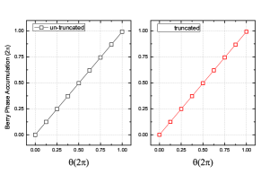
Figure 8: Winding of the accumulated Berry phase as a function of $\theta_{x}$, for (a) the untruncated ground state of $\nu=1$ non-Abelian Moore-Read state and (b) the corresponding truncated ground state. The accumulated Berry phase is defined in Eq. 43. Calculation is done with a flat-band model on a $2\times 3\times 4$ honeycomb lattice. Wang et al. (2012)

References

- Bernevig and Hughes (2013) B. A. Bernevig and T. L. Hughes, Topological Insulators and Topological Superconductors (Princeton University Press, 2013).
- Qi and Zhang (2011) X.-L. Qi and S.-C. Zhang, Rev. Mod. Phys. 83, 1057 (2011).
- Ryu et al. (2010) S. Ryu, A. P. Schnyder, A. Furusaki, and A. W. W. Ludwig, New Journal of Physics 12, 065010 (2010), eprint 0912.2157.
- Chiu et al. (2016) C.-K. Chiu, J. C. Y. Teo, A. P. Schnyder, and S. Ryu, Rev. Mod. Phys. 88, 035005 (2016).
- Hasan and Kane (2010) M. Z. Hasan and C. L. Kane, Rev. Mod. Phys. 82, 3045 (2010).
- Ando (2013) Y. Ando, Journal of the Physical Society of Japan 82, 102001 (2013), eprint 1304.5693.
- Bloch et al. (2008) I. Bloch, J. Dalibard, and W. Zwerger, Rev. Mod. Phys. 80, 885 (2008).
- Bloch et al. (2012) I. Bloch, J. Dalibard, and S. Nascimbène, Nature Physics 8, 267 (2012).
- Langen et al. (2015) T. Langen, R. Geiger, and J. Schmiedmayer, Annual Review of Condensed Matter Physics 6, 201 (2015), eprint 1408.6377.
- Thouless et al. (1982) D. J. Thouless, M. Kohmoto, M. P. Nightingale, and M. den Nijs, Phys. Rev. Lett. 49, 405 (1982).
- Zak (1989) J. Zak, Phys. Rev. Lett. 62, 2747 (1989).
- King-Smith and Vanderbilt (1993) R. D. King-Smith and D. Vanderbilt, Phys. Rev. B 47, 1651 (1993).
- Suzuki and Lee (1980) K. Suzuki and S. Y. Lee, Progress of Theoretical Physics 64, 2091 (1980).
- Anderson (1987) P. W. Anderson, Science 235, 1196 (1987).
- Gros (1989) C. Gros, Annals of Physics 189, 53 (1989).
- Schollwöck (2011) U. Schollwöck, Annals of Physics 326, 96 (2011), eprint 1008.3477.
- Wen (2002) X.-G. Wen, Phys. Rev. B 65, 165113 (2002).
- Niu et al. (1985) Q. Niu, D. J. Thouless, and Y.-S. Wu, Phys. Rev. B 31, 3372 (1985).
- Gu and Sun (2016) J. Gu and K. Sun, Phys. Rev. B 94, 125111 (2016), eprint 1605.07627.
- Huang and Balatsky (2016) Z. Huang and A. V. Balatsky, Phys. Rev. Lett. 117, 086802 (2016), eprint 1604.04698.
- Kohmoto (1985) M. Kohmoto, Annals of Physics 160, 343 (1985).
- Sheng et al. (2006) D. N. Sheng, Z. Y. Weng, L. Sheng, and F. D. M. Haldane, Phys. Rev. Lett. 97, 036808 (2006).
- Fukui and Hatsugai (2007) T. Fukui and Y. Hatsugai, Phys. Rev. B 75, 121403 (2007).
- Prodan (2009) E. Prodan, Phys. Rev. B 80, 125327 (2009).
- Yang et al. (2011) Y. Yang, Z. Xu, L. Sheng, B. Wang, D. Y. Xing, and D. N. Sheng, Phys. Rev. Lett. 107, 066602 (2011).
- Teo et al. (2008) J. C. Y. Teo, L. Fu, and C. L. Kane, Phys. Rev. B 78, 045426 (2008).
- Alexandradinata et al. (2014) A. Alexandradinata, C. Fang, M. J. Gilbert, and B. A. Bernevig, Phys. Rev. Lett. 113, 116403 (2014).
- Hughes et al. (2011) T. L. Hughes, E. Prodan, and B. A. Bernevig, Phys. Rev. B 83, 245132 (2011).
- McGreevy et al. (2012) J. McGreevy, B. Swingle, and K.-A. Tran, Phys. Rev. B 85, 125105 (2012).
- Lu and Ran (2012) Y.-M. Lu and Y. Ran, Phys. Rev. B 85, 165134 (2012).
- Zhang and Vishwanath (2013) Y. Zhang and A. Vishwanath, Phys. Rev. B 87, 161113 (2013).
- Hu et al. (2015) W.-J. Hu, W. Zhu, Y. Zhang, S. Gong, F. Becca, and D. N. Sheng, Phys. Rev. B 91, 041124 (2015).
- Kourtis et al. (2014) S. Kourtis, T. Neupert, C. Chamon, and C. Mudry, Phys. Rev. Lett. 112, 126806 (2014).
- Haldane (1983) F. D. M. Haldane, Phys. Rev. Lett. 50, 1153 (1983).
- Hirano et al. (2008) T. Hirano, H. Katsura, and Y. Hatsugai, Phys. Rev. B 77, 094431 (2008).
- Affleck et al. (1987) I. Affleck, T. Kennedy, E. H. Lieb, and H. Tasaki, Phys. Rev. Lett. 59, 799 (1987).
- Arovas et al. (1988) D. P. Arovas, R. N. Bhatt, F. D. M. Haldane, P. B. Littlewood, and R. Rammal, Phys. Rev. Lett. 60, 619 (1988).
- Rommelse and den Nijs (1987) K. Rommelse and M. den Nijs, Phys. Rev. Lett. 59, 2578 (1987).
- Girvin and Arovas (1989) S. M. Girvin and D. P. Arovas, Physica Scripta 1989, 156 (1989).
- Peschel (2003) I. Peschel, Journal of Physics A: Mathematical and General 36, L205 (2003).
- Cheong and Henley (2004) S.-A. Cheong and C. L. Henley, Phys. Rev. B 69, 075111 (2004).
- Li and Haldane (2008) H. Li and F. D. M. Haldane, Phys. Rev. Lett. 101, 010504 (2008).
- Thomale et al. (2010) R. Thomale, D. P. Arovas, and B. A. Bernevig, Phys. Rev. Lett. 105, 116805 (2010).
- Pollmann et al. (2010) F. Pollmann, A. M. Turner, E. Berg, and M. Oshikawa, Phys. Rev. B 81, 064439 (2010).
- Prodan et al. (2010) E. Prodan, T. L. Hughes, and B. A. Bernevig, Physical Review Letters 105, 115501 (2010), eprint 1005.5148.
- Huang and Arovas (2012) Z. Huang and D. P. Arovas, Phys. Rev. B 86, 245109 (2012), eprint 1201.0733.
- Hsieh and Fu (2014) T. H. Hsieh and L. Fu, Phys. Rev. Lett. 113, 106801 (2014).
- Fukui and Hatsugai (2014) T. Fukui and Y. Hatsugai, Journal of the Physical Society of Japan 83, 113705 (2014).
- Chiou et al. (2016) D.-W. Chiou, H.-C. Kao, and F.-L. Lin, Phys. Rev. B 94, 235129 (2016).
- Legner and Neupert (2013) M. Legner and T. Neupert, Phys. Rev. B 88, 115114 (2013).
- Schliemann (2013) J. Schliemann, New Journal of Physics 15, 053017 (2013), eprint 1302.5517.
- Hauke et al. (2014) P. Hauke, M. Lewenstein, and A. Eckardt, Physical Review Letters 113, 045303 (2014), eprint 1401.8240.
- Fläschner et al. (2016) N. Fläschner, B. S. Rem, M. Tarnowski, D. Vogel, D.-S. Lühmann, K. Sengstock, and C. Weitenberg, Science 352, 1091 (2016), eprint 1509.05763.
- Hofstadter (1976) D. R. Hofstadter, Phys. Rev. B 14, 2239 (1976).
- Bernevig et al. (2006) B. A. Bernevig, T. L. Hughes, and S.-C. Zhang, Science 314, 1757 (2006).
- Yu et al. (2011) R. Yu, X. L. Qi, A. Bernevig, Z. Fang, and X. Dai, Phys. Rev. B 84, 075119 (2011).
- Note (1) Note1, there are only distinctive terms for even and distinctive terms for odd , depending on whether or not the spin configuration is present in the expansion.
- (58) C. Weitenberg, Private communication.
- Wang et al. (2012) Y.-F. Wang, H. Yao, Z.-C. Gu, C.-D. Gong, and D. N. Sheng, Phys. Rev. Lett. 108, 126805 (2012).