Lagrangian Reachabililty

Abstract

We introduce LRT, a new Lagrangian-based ReachTube computation algorithm that conservatively approximates the set of reachable states of a nonlinear dynamical system. LRT makes use of the Cauchy-Green stretching factor (SF), which is derived from an over-approximation of the gradient of the solution-flows. The SF measures the discrepancy between two states propagated by the system solution from two initial states lying in a well-defined region, thereby allowing LRT to compute a reachtube with a ball-overestimate in a metric where the computed enclosure is as tight as possible. To evaluate its performance, we implemented a prototype of LRT in C++/Matlab, and ran it on a set of well-established benchmarks. Our results show that LRT compares very favorably with respect to the CAPD and Flow* tools.

1 Introduction

Bounded-time reachability analysis is an essential technique for ensuring the safety of emerging systems, such as cyber-physical systems (CPS) and controlled biological systems (CBS). However, computing the reachable states of CPS and CBS is a very difficult task as these systems are most often nonlinear, and their state-space is uncountably infinite. As such, these systems typically do not admit a closed-form solution that can be exploited during their analysis.

For CPS/CBS, one can therefore only compute point solutions (trajectories) through numerical integration and for predefined inputs. To cover the infinite set of states reachable by the system from an initial region, one needs to conservatively extend (symbolically surround) these pointwise solutions by enclosing them in reachtubes. Moreover, the starting regions of these reachtubes have to cover the initial states region.

The class of continuous dynamical systems we are interested in this paper are nonlinear, time-variant ordinary differential equations (ODEs):

$$x^{\prime}(t) =F(t,x(t)),$$ (1a)

$$x(t_{0}) =x_{0},$$ (1b)

where $x\colon\mathbb{R}\to\mathbb{R}^{n}$. We assume that $F$ is a smooth function, which guarantees short-time existence of solutions. The class of time-variant systems includes the class of time-invariant systems. Time-variant equations may contain additional terms, e.g. an excitation variable, and/or periodic forcing terms.

For a given initial time $t_{0}$, set of initial states $\mathcal{X}\subset\mathbb{R}^{n}$, and time bound $T>t_{0}$, our goal is to compute conservative reachtube of (1), that is, a sequence of time-stamped sets of states $(R_{1},t_{1}),\dots,(R_{k},t_{k})$ satisfying:

$$\text{Reach}\left((t_{0},\mathcal{X}\right),[t_{i-1},t_{i}])\subset R_{i}\text{ for }i=1,\dots,k,$$

where $\text{Reach}\left((t_{0},\mathcal{X}\right),[t_{i-1},t_{i}])$ denotes the set of reachable states of (1) in the interval $[t_{i-1},t_{i}]$. Whereas there are many sets satisfying this requirement, of particular interest to us are reasonably tight reachtubes; i.e. reachtubes whose over-approximation is the tightest possible, having in mind the goal of proving that a certain region of the phase space is (un)safe, and avoiding false positives. In practice and for the sake of comparision with other methods, we compute a discrete-time reachtube; as we discuss, a continuous reachtube can be obtained using our algorithm.

Existing tools and techniques for conservative reachtube computation can be classified by the time-space approximation they perform into three categories: (1) Taylor-expansion in time, variational-expansion in space (wrapping-effect reduction) of the solution set (CAPD [4, 32, 33], VNode-LP [26, 25], (2) Taylor-expansion in time and space of the solution set (Cosy Infinity [21, 3, 22], Flow* [5, 6]), and (3) Bloating-factor-based and discrepancy-function-based [10, 11]. The last technique computes a conservative reachtube using a discrepancy function (DF) that is derived from an over-approximation of the Jacobian of the vector field (usually given by the RHS of the differential equations) defining the continuous dynamical system.

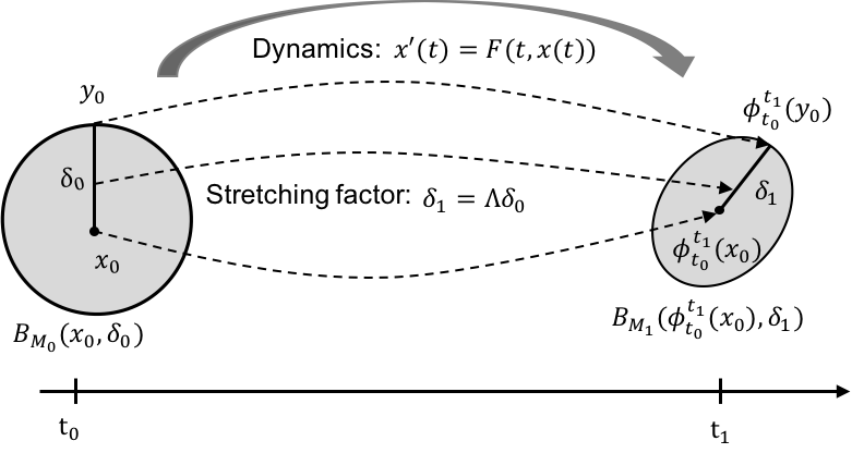
Figure 1: An overview of LRT. The figure shows one execution step of the LRT described in detail in Section 3. The dashed arrows reflect the solution flow $\phi$ and the evolution of state discrepancy.

This paper proposes an alternative (and orthogonal to [10, 11]) technique for computing a conservative reachtube, by using a stretching factor (SF) that is derived from an over-approximation of the gradient of the solution-flows, also referred to as the sensitivity matrix [8, 9], and the deformation tensor. An illustration of our method is given in Figure 1. $B_{M_{0}}(x_{0},\delta_{0})$ is a well-defined initial region given as a ball in metric space $M_{0}$ centered at $x_{0}$ of radius $\delta_{0}$. The SF $\Lambda$ measures the discrepancy of two states $x_{0}$, $y_{0}$ in $B_{M_{0}}$ propagated by the solution flow induced by (1), i.e. $\phi_{t_{0}}^{t_{1}}$. We can thus use the SF to bound the infinite set of reachable states at time $t_{1}$ with the ball-overestimate $B_{M_{1}}(\phi_{t_{0}}^{t_{1}}(x_{0}),\delta_{1})$ in an appropriate metric (which may differ from the initial $M_{0}$), where $\delta_{1}=\Lambda\cdot\delta_{0}$. Similar to [10], this metric is based on a weighted norm, yielding a tightest-possible enclosure of the reach-set [7, 19, 17, 20]. For two-dimensional system, we present an analytical method to compute $M_{1}$, but for higher dimensional system, we solve a semi-definite optimization problem. Analytical formulas derived for 2d case allow for faster computation. We point out that the output provided by LRT can be used to compute a validated bound for the so-called finite-time Lyapunov exponent ($FTLE=\frac{1}{T}\ln(SF)$) for a whole set of solutions. FTLE are widely computed in e.g. climate research in order to detect Lagrangian coherent structures.

We call this approach and its associated the LRT, for Lagrangian Reachtube computation. The LRT uses analogues of Cauchy-Green deformation tensors (CGD) from finite strain theory (FST) to determine the SF of the solution-flows, after each of its time-step iterations. The LRT algorithm is described thoroughly in Section 3.

To compute the gradient of the flows, we currently make use of the CAPD $C^{1}$ routine, which propagates the initial ball (box) using interval arithmetic. The CAPD library has been certified to compute a conservative enclosure of the true solution, and it has been used in many peer-reviewed computer proofs of theorems in dynamical systems, including [12, 15, 31].

To evaluate the LRT’s performance, we implemented a prototype in C++/Matlab and ran it on a set of eight benchmarks. Our results show that the LRT compares very favorably to a direct use of CAPD and Flow* (see Section 4), while still leaving room for further improvement. In general, we expect the LRT to behave favorably on systems that exhibit long-run stable behavior, such as orbital stability.

We did not compare the LRT with the DF-based tools [11, 10], although we would have liked to do this very much. The reason is that the publicly-available DF-prototype has not yet been certified to produce conservative results. Moreover, the prototype only considers time-invariant systems.

The rest of the paper is organized as follows. Section 2 reviews finite-strain theory and the Cauchy-Green-deformation tensor for flows. Section 3 presents the LRT, our main contribution, and proves that it conservatively computes the reachtube of a Cauchy system. Section 4 compares our results to CAPD and Flow* on six benchmarks from [6, 10], the forced Van der Pol oscillator (time-variant system) [30], and the Mitchell Schaeffer cardiac cell model [23]. Section 5 offers our concluding remarks and discusses future work.

2 Background on Flow Deformation

In this section we present some background on the LRT. First, in Section 2.1 we briefly recall the general FST, as in the LRT we deal with matrices analogous to Cauchy-Green deformation tensors. Second, in Section 2.2 we show how the Cauchy-Green deformation tensor can be used to measure discrepancy of two initial states propagated by the flow induced by Eq. (1).

2.1 Finite Strain Theory and Lagrangian Description of the Flow

In classical continuum mechanics, finite strain theory (FST) deals with the deformation of a continuum body in which both rotation and strain can be arbitrarily large. Changes in the configuration of the body are described by a displacement field. Displacement fields relate the initial configuration with the deformed configuration, which can be significantly different. FST has been applied, for example, in stress/deformation analysis of media like elastomers, plastically-deforming materials, and fluids, modeled by constitutive models (see e.g., [13], and the references provided there). In the Lagrangian representation, the coordinates describe the deformed configuration (in the material-reference-frame spatial coordinates), whereas in the Eulerian representation, the coordinates describe the undeformed configuration (in a fixed-reference-frame spatial coordinates).

Notation

In this section we use the standard notation used in the literature on FST. We use $X$ to denote the position of a particle in the Eulerian coordinates (undeformed), and $x$ to denote the position of a particle in the Lagrangian coordinates (deformed). The Lagrangian coordinates depend on the initial (Eulerian) position, and the time $t$, so we use $x(X,t)$ to denote the position of a particle in Lagrangian coordinates.

The displacement field from the initial configuration to the deformed configuration in Lagrangian coordinates is given by the following equation:

$$u(X,t)=x(X,t)-X.$$ (2)

The dependence $\nabla_{X}{u}$ of the displacement field $u(X,t)$ on the initial condition $X$ is called the material displacement gradient tensor, with

$$\nabla_{X}{u(X,t)}=\nabla_{X}{x}(X,t)-I,$$ (3)

where $\nabla_{X}{x}$ is called the deformation gradient tensor.

We now investigate how an initial perturbation $X+dX$ in the Eulerian coordinates evolves to the deformed configuration $dx(X+dX,t)$ in Lagrangian coordinates by using (2). This is called a relative displacement vector:

$$dx(X+dX,t)=x(X+dX,t)-x(X,t)=u(X+dX,t)+dX-u(X,t),$$

As a consequence, for small $dX$ we obtain the following approximate equality:

$$dx(X+dX,t)\approx u(X+dX,t)-u(X,t).$$ (4)

Now let us compute $u(X+dX,t)$ by expressing $du(X+dX,t)$ as with $x(X+dX,t)$ above. One obtains:

$$u(X+dX,t)=u(X,t)+du(X+dX,t)=u(X,t)+\nabla_{X}{u(X+dX,t)}dX.$$

Now by replacing $u(X+dX,t)$ in Equation (4) above, one obtains the following result:

$$dx(X+dX,t)\approx\nabla_{X}{x(X+dX,t)}dX.$$

Several rotation-independent tensors have been introduced in the literature. Classical examples include the right Cauchy-Green deformation tensor:

$$CG=\|\nabla_{X}{x}\|^{2}=(\nabla_{X}{x})^{T}\cdot\nabla_{X}{x}.$$ (5)

2.2 Cauchy-Green Deformation Tensor for Flows

Notation

By $[x]$ we denote a product of intervals (a box), i.e. a compact and connected set $[x]\subset\mathbb{R}^{n}$. We will use the same notation for interval matrices. By $\|\cdot\|_{2}$ we denote the Euclidean norm, by $\|\cdot\|_{\infty}$ we denote the max norm, we use the same notation for the induced operator norms. Let $B(x,\delta)$ denote the closed ball centered at $x$ with the radius $\delta$. It will be clear from the context in which metric space we consider the ball. By $\phi_{t_{0}}^{t_{1}}$ we denote the flow induced by (1), by $D_{x}\phi_{t_{0}}^{t_{1}}$ we denote the partial derivative in $x$ of the flow with respect to the initial condition, at time $t_{1}$, which we call the gradient of the flow, also referred to as the sensitivity matrix [8, 9].

Let us now relate the finite strain theory presented in Section 2.1 to the study of flows induced by the ODE (1). For expressing deformation in time of a continuum we first consider the set of initial conditions (e.g. a ball), which is being evolved (deformed) in time by the flow $\phi$. For the case of flows we have that the positions in Eulerian coordinates are coordinates of the initial condition (denoted here using lower case letters with subscript $0$, i.e. $x_{0}$, $y_{0}$). The equivalent of $x(X,t)$ – the Lagrangian coordinates of $X$ at time $t$ – is $\phi_{t_{0}}^{t}(x_{0})$. Obviously, the equivalent of $u(X,t)$ is $(\phi_{t_{0}}^{t}(x_{0})-x_{0})$, and the deformation gradient $\nabla_{X}{x}$ here is just the derivative of the flow with respect to the initial condition $D_{x}\phi_{t_{0}}^{t}$ (sensitivity matrix).

In this section we show that deformation tensors arise in a study of discrepancy of solutions of (1). First, we provide some basic lemmas that we use in the analysis of our reachtube-computation algorithm. We work with the metric spaces that are based on weighted norms. We aim at finding weights, such that the induced weighted norms provides to be smaller than those in the Euclidean norm for the computed gradients of solutions. This procedure is similar to finding appropriate induced matrix measures (also known as logarithmic norms), which provides rate of expansion between two solutions, see [7, 19, 17, 20].

Definition 1

Given positive-definite symmetric matrix $M\in\mathbb{R}^{n\times n}$ we define the $M$-norm of $\mathbb{R}^{n}$ vectors by

$$\|y\|_{M}=\sqrt{y^{T}My}.$$ (6)

Given the decomposition

$$M=C^{T}C,$$

the matrix norm induced by (6) is

$$\|A\|_{M}=\sqrt{\lambda_{max}\left((C^{T})^{-1}\cdot A^{T}\cdot M\cdot A\cdot C^{-1}\right)},$$ (7)

where $\lambda_{max}(\cdot)$ denotes the maximal eigenvalue.

Observe that the square-root is well defined, as $\lambda_{max}\,{\geq}\,0$, because $M$ is symmetric semi-positive definite, and hence, the matrix $(C^{T})^{-1}\cdot A^{T}\cdot M\cdot A\cdot C^{-1}$ is also symmetric semi-positive definite.

Lemma 1

Consider the Cauchy problem (1). Let $x_{0},y_{0}\in\mathbb{R}^{n}$ be two initial conditions at time $t_{0}$. Let $M\in\mathbb{R}^{n\times n}$ be a positive-definite symmetric matrix and $C^{T}C=M$ be its decomposition. For $t_{1}\geq t_{0}$, it holds that

$$\|\phi_{t_{0}}^{t_{1}}(x_{0}){-}\phi_{t_{0}}^{t_{1}}(y_{0})\|_{M}\,{\leq}\,\sqrt{\lambda_{max}\left((C^{T})^{-1}D_{x}\phi_{t_{0}}^{t_{1}}(\xi)^{T}M\,D_{x}\phi_{t_{0}}^{t_{1}}(\xi)C^{-1}\right)}~{}\|x_{0}-y_{0}\|_{M}$$ (8)

where $\xi=\omega x_{0}+(1-\omega)y_{0}$ for some $\omega\in[0,1]$. For the particular case of the Euclidean norm, (8) takes the form

$$\|\phi_{t_{0}}^{t_{1}}(x_{0})-\phi_{t_{0}}^{t_{1}}(y_{0})\|_{2}\leq\sqrt{\lambda_{max}\left(\left(D_{x}\phi_{t_{0}}^{t_{1}}(\xi)\right)^{T}\cdot D_{x}\phi_{t_{0}}^{t_{1}}(\xi)\right)}~{}\|x_{0}-y_{0}\|_{2}.$$ (9)

A proof can be found in Appendix 0.A.

Remark 1

Let $\xi\in\mathbb{R}$ be a given vector. Observe that $\left(D_{x}\phi_{t_{0}}^{t_{1}}(\xi)\right)^{T}\cdot D_{x}\phi_{t_{0}}^{t_{1}}(\xi)$ appearing in (9) is the right Cauchy-Green deformation tensor (5) for two given initial vectors $x_{0}$ and $y_{0}$. We call the value $\sqrt{\lambda_{max}}$ appearing in (9) Cauchy-Green stretching factor for given initial vectors $x_{0}$ and $y_{0}$, which is necessarily positive as the CG deformation tensor is positive definite $\sqrt{\lambda_{max}(\cdot)}>0$.

Lemma 1 is used when both of the discrepancy of the solutions at time $t_{1}$ as well as the initial conditions is measured in the same $M$-norm. In the practical Lagrangian Reachtube Algorithm the norm used is changed during the computation. Hence we need another version of Lemma 1, where the norm in which the discrepancy of the initial condition in measured differs from the norm in which the discrepancy of the solutions at time $t_{1}$ is measured.

Lemma 2

Consider the Cauchy problem (1). Let $x_{0},y_{0}\in\mathbb{R}^{n}$ be two initial conditions at time $t_{0}$. Let $M_{0},M_{1}\in\mathbb{R}^{n\times n}$ be positive-definite symmetric matrices, and $C_{0}^{T}C_{0}=M_{0}$, $C_{1}^{T}C_{1}=M_{1}$ their decompositions respectively. For $t_{1}\geq t_{0}$, it holds that

$$\|\phi_{t_{0}}^{t_{1}}(x_{0})-\phi_{t_{0}}^{t_{1}}(y_{0})\|_{M_{1}}\\ \leq\sqrt{\lambda_{max}\left((C_{0}^{T})^{-1}\cdot\left(D_{x}\phi_{t_{0}}^{t_{1}}(\xi)\right)^{T}\cdot M_{1}\cdot D_{x}\phi_{t_{0}}^{t_{1}}(\xi)\cdot C_{0}^{-1}\right)}~{}\|x_{0}-y_{0}\|_{M_{0}},$$ (10)

where $\xi=\omega x_{0}+(1-\omega)y_{0}$ for some $\omega\in[0,1]$.

A proof can be found in Appendix 0.A.

Remark 2

Given a positive-definite symmetric matrix $M$. We call the value appearing in (10) $(C_{0}^{T})^{-1}\cdot\left(D_{x}\phi_{t_{0}}^{t_{1}}(\xi)\right)^{T}\cdot M_{1}\cdot D_{x}\phi_{t_{0}}^{t_{1}}(\xi)\cdot C_{0}^{-1}$ as the $M_{0}/M_{1}$-deformation tensor, and the value $\sqrt{\lambda_{max}}$ as the $M_{0}/M_{1}$-stretching factor.

The idea behind using weighted norms in our approach is that the stretching factor in $M$-norm (10) is expected to be smaller than that in the Euclidean norm (9). Ultimately, this permits a tighter reachtube computation, whose complete procedure is presented in Section 3.3.

3 Lagrangian Reachtube Computation

3.1 Reachtube Computation: Problem-Statement

In this section we provide first some lemmas that we then use to show that our method-and-algorithm produces a conservative output, in the sense that it encloses the set of solutions starting from a set of initial conditions. Precisely, we define what we mean by conservative enclosures.

Definition 2

Given an initial set $\mathcal{X}$, initial time $t_{0}$, and the target time $t_{1}\geq t_{0}$. We call the following compact sets:

• $\mathcal{W}\subset\mathbb{R}^{n}$ a conservative, reach-set enclosure, if $\phi_{t_{0}}^{t_{1}}(x)\in\mathcal{W}$ for all $x\in\mathcal{X}$.

• $\mathcal{D}\subset\mathbb{R}^{n\times n}$ a conservative, gradient enclosure, if $D_{x}\phi_{t_{0}}^{t_{1}}(x)\in\mathcal{D}$ for all $x\in\mathcal{X}$.

Following the notation used in [10], and extending the corresponding definitions to our time variant setting, we introduce the notion of reachibility as follows: Given an initial set $\mathcal{X}\subset\mathbb{R}^{n}$ and a time $t_{0}$, we call a state $x$ in $\mathbb{R}^{n}$ as reachable within a time interval $[t_{1},t_{2}]$, if there exists an initial state $x_{0}\in\mathcal{X}$ at time $t_{0}$ and a time $t\in[t_{1},t_{2}]$, such that $x=\phi_{t_{0}}^{t}(x_{0})$. The set of all reachable states in the interval $[t_{1},t_{2}]$ is called the reach set and is denoted by $\mbox{Reach}((t_{0},\mathcal{X}),[t_{1},t_{2}])$.

Definition 3 ([10] Def. 2.4)

Given an initial set $\mathcal{X}$, initial time $t_{0}$, and a time bound $T$, a $((t_{0},X),T)$-reachtube of System (1) is a sequence of time-stamped sets $(R_{1},t_{1}),\dots,(R_{k},t_{k})$ satisfying the following: (1) $t_{0}\leq t_{1}\leq\dots\leq t_{k}=T$, (2) $\mbox{Reach}((t_{0},\mathcal{X}),[t_{i-1},t_{i}])\subset R_{i},\forall i=1,\dots,k$.

Definition 4

Whenever the initial set $\mathcal{X}$ and the time horizon $T$ are known from the context we will skip the $(\mathcal{X},[t_{0},T])$ part, and will simply use the name (conservative) reachtube over-approximation of the flow defined by (1).

Observe that we do not address here the question what is the exact structure of the solution set at time $t$ initiating at $\mathcal{X}$. In general it could have, for instance, a fractal structure. We aim at constructing an over-approximation for the solution set, and its gradient, which is amenable for rigorous numeric computations.

In the theorems below we show that the method presented in this paper can be used to construct a reachtube over-approximation $\mathcal{R}$. The theorems below is the foundation of our novel Lagrangian Reachtube Algorithm (LRT) presented in Section 3.3. In particular, the theorems below provide estimates we use for constructing $\mathcal{R}$. First, we present a theorem for the discrete case.

3.2 Conservative Reachtube Construction

Theorem 3.1

Let $t_{0}\leq t_{1}$ be two time points. Let $\phi_{t_{0}}^{t_{1}}(x)$ be the solution of (1) with the initial condition $(t_{0},x)$ at time $t_{1}$, let $D_{x}\phi_{t_{0}}^{t_{1}}$ be the gradient of the flow. Let $M_{0},M_{1}\in\mathbb{R}^{n\times n}$ be positive-definite symmetric matrices, and $C_{0}^{T}C_{0}=M_{0}$, $C_{1}^{T}C_{1}=M_{1}$ be their decompositions respectively. Let $\mathcal{X}=B_{M_{0}}(x_{0},\delta_{0})\subset\mathbb{R}^{n}$ be a set of initial states for the Cauchy problem (1) (ball in $M_{0}$-norm with the center at $x_{0}$, and radius $\delta_{0}$). Assume that there exists a compact, conservative enclosure $\mathcal{D}\subset\mathbb{R}^{n\times n}$ for the gradients, such that:

$$D_{x}\phi_{t_{0}}^{t_{1}}(x)\in\mathcal{D}\text{ for all }x\in\mathcal{X}.$$ (11)

Suppose $\Lambda>0$ is such that:

$$\Lambda\geq\sqrt{\lambda_{max}\left((C_{0}^{T})^{-1}D^{T}M_{1}DC^{-1}_{0}\right)},\text{ for all }D\in\mathcal{D}.$$ (12)

Then it holds that:

$$\phi_{t_{0}}^{t_{1}}(x)\in B_{M_{1}}(\phi_{t_{0}}^{t_{1}}(x_{0}),\Lambda\cdot\delta_{0}).$$

Proof

Let $x_{0}$ be the center of the ball of initial conditions $\mathcal{X}=B_{M_{0}}(x_{0},\delta_{0})$, and let us pick $x\in\mathcal{X}$. From Lemma 4 the discrepancy of the solutions initiating at $x_{0}$ and $x$ at time $t_{1}$ is bounded in $M_{1}$-norm by:

$$\|\phi_{t_{0}}^{t_{1}}(x_{0})-\phi_{t_{0}}^{t_{1}}(x)\|_{M_{1}}\leq\delta_{0}\sqrt{\lambda_{max}\left((C_{0}^{T})^{-1}\cdot\left(D_{x}\phi_{t_{0}}^{t_{1}}(\xi)\right)^{T}\cdot M_{1}\cdot D_{x}\phi_{t_{0}}^{t_{1}}(\xi)\cdot C_{0}^{-1}\right)},$$

where $\xi=\omega x_{0}+(1-\omega)x$ for some $\omega\in[0,1]$. Obviously, $\xi\in B_{M_{0}}(x_{0},\delta_{0})$. Hence, $D_{x}\phi_{t_{0}}^{t_{1}}(\xi)\in\mathcal{D}.$ Moreover, if $\Lambda>0$ satisfies (12), then

$$\Lambda\geq\sqrt{\lambda_{max}\left((C_{0}^{T})^{-1}\cdot\left(D_{x}\phi_{t_{0}}^{t_{1}}(\xi)\right)^{T}\cdot M_{1}\cdot D_{x}\phi_{t_{0}}^{t_{1}}(\xi)\cdot C_{0}^{-1}\right)},$$

and $\phi_{t_{0}}^{t_{1}}(x)\in B_{M_{1}}(\phi_{t_{0}}^{t_{1}}(x_{0}),\Lambda\delta_{0}).$ As $x$ was chosen in an arbitrary way, we are done. ∎

The next theorem is the variant of Theorem 3.1 for obtaining a continuous reachtube.

Theorem 3.2

Let $\phi_{t_{0}}^{t_{1}}(x)$ be the solution of (1) with the initial condition $(t_{0},x)$ at time $t_{1}$, let $D_{x}\phi_{t_{0}}^{t_{1}}$ be the gradient of the flow. Let $M_{0},M_{1}\in\mathbb{R}^{n\times n}$ be positive definite symmetric matrices, and $C_{0}^{T}C_{0}=M_{0}$, $C_{1}^{T}C_{1}=M_{1}$ be their decompositions respectively. Let $\mathcal{X}=B_{M_{0}}(x_{0},\delta_{0})\subset\mathbb{R}^{n}$ be a set of initial conditions for the Cauchy problem (1) (ball in $M_{0}$-norm). Assume that there exists $\{\mathcal{D}_{t}\}_{t\in[t_{0},t_{1}]}$ – a compact $t$-parametrized set, such that

$$\mathcal{D}_{t}\subset\mathbb{R}^{n\times n}\text{ for }t\in[t_{0},t_{1}],$$

$$D_{x}\phi_{t_{0}}^{t}(x)\in\mathcal{D}_{t}\text{ for all }x\in\mathcal{X}\text{, and }t\in[t_{0},t_{1}].$$

If $\Lambda>0$ is such that $\text{for all }D\colon D\in\mathcal{D}_{t}\text{ for some }t\in[t_{0},t_{1}]$

$$\Lambda\geq\sqrt{\lambda_{max}\left((C_{0}^{T})^{-1}D^{T}M_{1}DC^{-1}_{0}\right)}$$

Then for all $t\in[t_{0},t_{1}]$ it holds that

$$\phi_{t_{0}}^{t}(x)\in B_{M_{1}}(\phi_{t_{0}}^{t}(x_{0}),\Lambda\cdot\delta_{0}).$$ (13)

Proof

It follows from the proof of Theorem 3.1 applied to all times $t\in[t_{0},t_{1}]$. ∎

Corollary 1

Let $T\geq t_{0}$. Assume that that there exists $\{\mathcal{D}_{t}\}_{t\in[t_{0},T]}$ – a compact $t$-parametrized set, such that

$$\mathcal{D}_{t}\subset\mathbb{R}^{n\times n}\text{ for }t\in[t_{0},T],$$

$$D_{x}\phi_{t_{0}}^{t}(x)\in\mathcal{D}_{t}\text{ for all }x\in\mathcal{X}\text{, and }t\in[t_{0},T].$$

Then the existence of a $((t_{0},X),T)$-reachtube of the system described in Eq. (1) in sense of Definition 3, i.e. a sequence of time-stamped sets $(R_{1},t_{1}),\dots,(R_{k},t_{k})$ is provided by an application of Lemma 3.2. We provide an algorithm computing the reachtube in Section 3.3.

Proof

Immediate application of Theorem 3.2 shows that if the first segment $(R_{1},t_{1})$ is defined

$$(R_{1},t_{1}):=\bigcup_{t\in[t_{0},t_{1}]}{B_{M_{1}}(\phi_{t_{0}}^{t}(x_{0}),\Lambda\cdot\delta_{0})},$$

then it satisfies

$$\mbox{Reach}((t_{0},\mathcal{X}),[t_{0},t_{1}])\subset(R_{1},t_{1}),$$

which is exactly provided by (13). The $j$-th segment $(R_{j},t_{j})$ for $j=2,\dots,k$ is obtained by replacing in Theorem 3.2 the time interval $[t_{0},t_{1}]$ with the interval $[t_{j-1},t_{j}]$ (Observe that the norm may be different in each step). ∎

3.3 LRT: A Rigorous Lagrangian Computation Algorithm

We now present a complete description of our algorithm. In the next section we prove its correctness. First let us comment on how in practice we compute a representable enclosure for the gradients (11).

• First, given an initial ball $B_{M_{0}}(x_{0},\delta_{0})$ we compute its representable over-approximation, i.e., a product of intervals (a box in canonical coordinates $[X]\subset\mathbb{R}^{n}$), such that $B_{M_{0}}(x_{0},\delta_{0})\subset[X]$.

• Next, using the $C^{1}$-CAPD algorithm [33, 32] all trajectories initiating in $[X]$ are rigorously propagated forward in time, in order to compute a conservative enclosure for $\left\{D_{x}\phi_{t_{0}}^{t_{1}}(\xi)|\ \xi\in[X]\right\},$ the gradients. We use the notation $[D_{x}\phi_{t_{0}}^{t_{1}}([X])]\subset\mathbb{R}^{n\times n},$ to denote a representable enclosure (an interval matrix) for the set of gradients $\left\{D_{x}\phi_{t_{0}}^{t_{1}}(\xi)|\ \xi\in[X]\right\}.$

The norm of an interval vector $\|[x]\|$ is defined as the supremum of the norms of all vectors within the bounds $[x]$. For an interval set $[x]\subset\mathbb{R}^{n}$ we denote by $\mathbb{R}^{n}\supset B_{M}([x],r):=\bigcup_{x\in[x]}{B_{M}(x,r)}$, the union of the balls in $M$-norm of radius $r$ having the center in $[x]$. Each product of two interval matrices is overestimated by using the interval-arithmetic operations.

Definition 5

We will call the $C^{1}$-CAPD algorithm the rigorous tool, which is currently used to generate conservative enclosures for the gradient in the LRT.

The output of the LRT are discrete-time reachtube over-approximation cross-sections $\{t_{0},t_{1},\dots,t_{k}\}$, $t_{k}\,{=}\,t_{0}\,{+}\,kT$, i.e., reachtube over-approximations $B_{M_{j}}(x_{j},\delta_{j})$ of the flow induced by (1) at time $t_{j}$. We note that the algorithm can be easily modified to provide a validated bounds for the finite-time Laypunov exponent. We use the discrete-time output for the sake of comparison. However, as a byproduct, a continuous reachtube over-approximation is obtained by means of rough enclosures (Fig. 2) produced by the rigorous tool used and by applying Theorem 3.2. The implementation details of the algorithm can be found in Section 4.

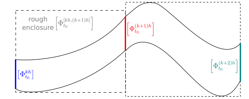
Figure 2: Fine bounds provided at equally spaced time steps (colored), and coarse bounds provided for the intermediate times by the rough enclosure (dotted boxes).

We are now ready to give the formal description of the LRT: (1) its inputs, (2) its outputs, and (3) its computation.

LRT: The Lagrangian Reachtube Algorithm
Input:

• ODEs (1): time-variant ordinary differential equations,

• $T$: time horizon, $t_{0}$: initial time, $k$: number of steps, $h\,{=}\,T{/}k$: time step

• $M_{0}$: initial positive-definite symmetric matrix defining the norm (6),

• $[x_{0}]\subset\mathbb{R}^{n}$: the initial bounds for the position of the center of the ball at $t_{0}$,

• $\delta_{0}>0$: the radius of the ball (in $M_{0}$ norm) about $x_{0}$ at $t_{0}$.
  

Output:

• $\{[x_{j}]\}_{j=1}^{k}\,{\subset}\,\mathbb{R}^{n\times{k}}$: interval enclosures for ball centers $x_{j}$ at time $t_{0}\,{+}\,jh$,

• $\{M_{j}\}_{j=1}^{k}$: norms defining metric spaces for the ball enclosures,

• $\{\delta_{j}\}_{j=1}^{k}\,{\in}\,\mathbb{R}_{+}^{k}$: radii of the ball enclosures at $x_{j}$ for $j=1,\dots,k$.

Begin LRT

1. Set $t_{1}\,{=}\,t_{0}\,{+}\,h$. Propagate the center of the ball $[x_{0}]$ forward in time by the time-step $h$, using the rigorous tool. The result is a conservative enclosure for the solutions $[\phi_{t_{0}}^{t_{1}}([x_{0}])]$ and the gradients $[D_{x}\phi_{t_{0}}^{t_{1}}([x_{0}])]$.

2. Choose a matrix $D\in[D_{x}\phi_{t_{0}}^{t_{1}}([x_{0}])]$, and compute a symmetric positive-definite matrix $M_{1}$, and its decomposition $M_{1}=C_{1}^{T}C_{1}$, such that, it minimizes the stretching factor for $D$. In other words, it holds that:

   $$\sqrt{\lambda_{max}\left((C_{1}^{T})^{-1}D^{T}M_{1}DC_{1}^{-1}\right)}\leq\sqrt{\lambda_{max}\left((\widetilde{C}^{T})^{-1}D^{T}\widetilde{M}D\widetilde{C}^{-1}\right)},$$ (14)

   for all positive-definite symmetric matrices $\widetilde{M}$. In the actual code we find the minimum with some resolution, i.e., we compute $M_{1}$, such that it is close to the optimal in the sense of (18), using the procedure presented in subsection 3.6.

3. Decide whether to change the norm of the ball enclosure from $M_{0}$ to $M_{1}$ (if it leads to a smaller stretching factor). If the norm is to be changed keep $M_{1}$ as it is, otherwise $M_{1}=M_{0}$,

4. Compute an over-approximation for $B_{M_{0}}([x_{0}],\delta_{0})$, which is representable in the rigorous tool employed by the LRT, and can be used as input to propagate forward in time all solutions initiating in $B_{M_{0}}([x_{0}],\delta_{0})$. This is a product of intervals in canonical coordinates $[X]\subset\mathbb{R}^{n}$, such that:

   $$B_{M_{0}}([x_{0}],\delta_{0})\subset[X].$$

   We compute the over-approximation using the interval arithmetic expression:

   $${C_{0}^{-1}(C_{0}\cdot[x_{0}]+[-\delta_{0},\delta_{0}]^{n})}$$

5. Rigorously propagate $[X]$ forward in time, using the rigorous tool over the time interval $[t_{0},t_{1}]$. The result is a continuous reachtube, providing bounds for $[\phi_{t_{0}}^{t}([X])]$, and $[D_{x}\phi_{t_{0}}^{t}([X])]$ for all $t\in[t_{0},t_{1}]$. We employ an integration algorithm with a fixed time-step $h$. As a consequence "fine" bounds are obtained for $t=t_{1}$. We denote those bounds by:

   $$[\phi_{t_{0}}^{t_{1}}([X])],\quad[D_{x}\phi_{t_{0}}^{t_{1}}([X])].$$

   We remark that for the intermediate time-bounds, i.e., for:

   $$[\phi_{t_{0}}^{t}([X])]\text{, for }t\in\left(t_{0},t_{1}\right),$$ (15)

   the so-called rough enclosures can be used. These provide coarse bounds, as graphically illustrated in Figure 2 in the appendix.

6. Compute interval matrix bounds for the $M_{0}/M_{1}$ Cauchy-Green deformation tensors:

   $$\left[\left((C^{T}_{0})^{-1}\cdot\left[D_{x}\phi_{t_{0}}^{t_{1}}([X])\right]^{T}\cdot C_{1}^{T}\right)\cdot\left(C_{1}\cdot\left[D_{x}\phi_{t_{0}}^{t_{1}}([X])\right]\cdot C^{-1}_{0}\right)\right],$$ (16)

   where $C^{T}_{0},C_{0}$ are s.t. $C^{T}_{0}C_{0}=M_{0}$, and $C^{T}_{1},C_{1}$ are s.t. $C^{T}_{1}C^{T}=M_{1}$. The interval matrix operations are executed in the order given by the brackets.

7. Compute a value $\Lambda>0$ ($M_{0}/M_{1}$ stretching factor) as an upper bound for the square-root of the maximal eigenvalue of each (symmetric) matrix in (16):

   $$\Lambda\geq\sqrt{\lambda_{max}\left(C\right)},$$

   $$\text{for all }C\in\left[\left((C^{T}_{0})^{-1}\cdot\left[D_{x}\phi_{t_{0}}^{t_{1}}([X])\right]^{T}\cdot C_{1}^{T}\right)\cdot\left(C_{1}\cdot\left[D_{x}\phi_{t_{0}}^{t_{1}}([X])\right]\cdot C^{-1}_{0}\right)\right].$$

   This quantity $\Lambda$ can be used for the purpose of computation of validated bound for the finite-time Lyapunov exponent

   $$FTLE(B_{M_{0}}([x_{0}],\delta_{0}))=\frac{1}{t_{1}-t_{0}}\ln(\Lambda_{prev}\cdot\Lambda),$$

   where $\Lambda_{prev}$ is the product of all stretching factors computed in previous steps.

8. Compute the new radius for the ball at time $t_{1}\,{=}\,t_{0}\,{+}\,h$:

   $$\delta(t_{1})=\Lambda\cdot\delta(t_{0}),$$

9. Set the new center of the ball at time $t_{1}$ as follows:

   $$[x_{1}]=[\phi_{t_{0}}^{t_{1}}([x_{0}])].$$

10. Set the initial time to $t_{1}$, the bounds for the initial center of the ball to $[x_{1}]$, the current norm to $M_{1}$, the radius in $M_{1}$-norm to $\delta_{1}\,{=}\,\Lambda\cdot\delta_{0}$, and the ball enclosure for the set of initial states to $B_{M_{1}}([x_{1}],\Lambda\cdot\delta(t_{0}))$. If $t_{1}\geq T$ terminate. Otherwise go back to 1.

End LRT

3.4 LRT-Algorithm Correctness Proof

In this section we provide a proof that the LRT, our new reachtube-computation algorithm, is an overapproximation of the behavior of the system described by Equations (1). This main result is captured by the following theorem.

Theorem 3.3 (LRT-Conservativity)

Assume that the rigorous tool used in the Lagrangian Reachtube Algorithm (LRT) produces conservative gradient enclosures for system (1) in the sense of Definition 2, and it guarantees the existence of the solutions within time intervals. Assume also that the LRT terminates on the provided inputs.

Then, the output of the LRT is a conservative reachtube over-approximation of (1) at times $\{t_{j}\}_{j=0}^{k}$, that is:

$$\mbox{Reach}((t_{0},\mathcal{X}),t_{j})\subset B_{M_{j}}([x_{j}],\delta_{j})\text{, for }j=1,\dots,k,$$

bounded solutions exists for all intermediate times $t\in(t_{j},t_{j+1})$.

Proof

Let $\mathcal{X}=B_{M_{0}}([x_{0}],\delta_{0})$ be a ball enclosure for the set of initial states. Without loosing generality we analyze the first step of the algorithm. The same argument applies to the consecutive steps (with the initial condition changed appropriately, as explained in the last step of the algorithm).

The representable enclosure $[X]\subset\mathbb{R}^{n}$ (product of intervals in canonical coordinates) computed in Step 4 satisfies $B_{M_{0}}([x_{0}],\delta_{0})\subset[X]$. By the assumption the rigorous-tool used produces conservative enclosures for the gradient of the flow induced by ODEs (1). Hence, as the set $[X]$ containing $B_{M_{0}}([x_{0}],\delta_{0})$ is the input to the rigorous forward-time integration procedure in Step 5, for the gradient enclosure $[D_{x}\phi_{t_{0}}^{t_{1}}([X])]$ computed in Step 5, it holds that

$$\left\{D_{x}\phi_{t_{0}}^{t_{1}}(x)\text{ for all }x\in\mathcal{X}\right\}\subset[D_{x}\phi_{t_{0}}^{t_{1}}([X])].$$

Therefore, the set $[D_{x}\phi_{t_{0}}^{t_{1}}([X])]$ can be interpreted as the set $\mathcal{D}$, i.e., the compact set containing all gradients of the solution at time $t_{1}$ with initial condition in $B_{M_{0}}([x_{0}],\delta_{0})$ appearing in Theorem 3.1, see (11). As a consequence, the value $\Lambda$ computed in Step 7 satisfies the following inequality:

$$\Lambda\geq\sqrt{\lambda_{max}\left((C_{1}^{T})^{-1}D^{T}M_{0}DC^{-1}_{1}\right)},\text{ for all }D\in\mathcal{D}.$$

From Theorem 3.2 it follows that:

$$\phi_{t_{0}}^{t_{1}}(x)\in B_{M_{1}}(\phi_{t_{0}}^{t_{1}}([x_{0}]),\Lambda\cdot\delta(t_{0}))\text{ for all }x\in\mathcal{X},$$

which implies that:

$$\mbox{Reach}((t_{0},\mathcal{X}),t_{1})\subset B_{M_{1}}([\phi_{t_{0}}^{t_{1}}([x_{0}])],\Lambda\cdot\delta(t_{0}))$$

which proves our overapproximation (conservativity) claim. Existence of the solutions for all times $t\in(t_{0},t_{1})$ is guaranteed by the assumption about the rigorous tool (in the step 5 of the LRT algorithm we use rough enclosures, see Figure 2). ∎

3.5 Wrapping Effect in the Algorithm

A very important precision-loss issue of conservative approximations, and therefore of validated methods for ODEs, is the wrapping effect. This occurs when a set of states is wrapped (conservatively enclosed) within a box defined in a particular norm. The weighted $M$-norms technique the LRT uses (instead of the standard Euclidean norm) is a way of reducing the effect of wrapping. More precisely, in Step 7 of every iteration, the LRT finds an appropriate norm which minimizes the stretching factor computed from the set of Cauchy-Green deformation tensors.

However, there are other sources of the wrapping effect in the algorithm. The discrete reachtube bounds are in a form of a ball in appropriate metric space, which is an ellipsoidal set in canonical coordinates, see example on Fig. 3a. In Step 4 of the LRT algorithm, a representable enclosure in canonical coordinates for the ellipsoidal reachtube over-approximation is computed. When the ellipsoidal set is being directly wrapped into a box in canonical coordinates (how it is done in the algorithm currently), the wrapping effect is considerably larger than when the ellipsoidal set is wrapped into a rectangular set reflecting the eigen-coordinates. We illustrate the wrapping effect using the following weighted norm (taken from one of our experiments):

$$M=\begin{bmatrix}7&-9.5\\ -9.5&19\end{bmatrix}$$ (17)

Figure 3 shows the computation of enclosures for a ball represented in the weighted norm given by $M$. It is clear from Figure 1(c) that the box enclosure of the ball in the eigen-coordinates (blue rectangle) is much tighter than the box enclosure of it in the canonical coordinates (green square).

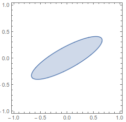
(a)

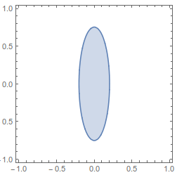
(b)

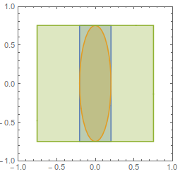
(c)

Figure 3: (a) A ball in the weighted norm given by $M$ of radius $1$ (the ellipsoidal set). (b) The ellipsoidal set in its eigen-coordinates (unrotated). (c) Wrapping the ellipsoidal set in a box: blue rectangle in eigen-coordinates and green square in canonical-coordinates.

Step 6 of the LRT is another place where reducing the wrapping effect has the potential to considerably increase the precision of the LRT. This step computes the product of interval matrices, which results in large overapproximations for wide-intervals matrices. In fact, in the experiments considered in Section 4, if the initial-ball radius is large, we observed that the overestimate of the stretching factor tends to worsen the LRT performance in reachtube construction, when compared to a direct application of CAPD and Flow*. We plan to find workarounds for this problem. One possible solution would be to use matrix decomposition, and compute the eigenvalues of the matrix by using this decomposition.

3.6 Direct computation of the optimal $M$-norm

The computation of the optimal $M$-norm enables the estimation of the streching factor. Step 7 of the LRT finds norm $M_{1}$ and decomposes it as $M_{1}=C_{1}^{T}C_{1}$, such that, for a gradient matrix $D$ the following inequality holds for all positive-definite symmetric matrices $\widetilde{M}$:

$$\sqrt{\lambda_{max}\left((C_{1}^{T})^{-1}D^{T}M_{1}DC_{1}^{-1}\right)}\leq\sqrt{\lambda_{max}\left((\widetilde{C}^{T})^{-1}D^{T}\widetilde{M}D\widetilde{C}^{-1}\right)},$$ (18)

Below we illustrate how to compute $M_{1}$ for 2D systems. This can be generalized to higher-dimensional systems.

I) $\mathbf{D}$ has complex conjugate eigenvalues $\mathbf{\lambda}\,\mathbf{=}\,\mathbf{\alpha}\,\mathbf{\pm}\,\mathbf{i}\mathbf{\beta}$.

In this case $w\pm iv$ is the associated pair of complex conjugate eigenvectors, where $w,v\in\mathbb{R}^{2}$. Define:

$$C=\begin{bmatrix}w&v\end{bmatrix}^{-1}$$

As a consequence we have the following equations:

$$CDC^{-1}=\begin{bmatrix}\alpha&\beta\\ -\beta&\alpha\end{bmatrix},\text{ and }(C^{T})^{-1}D^{T}C^{T}=\begin{bmatrix}\alpha&-\beta\\ \beta&\alpha\end{bmatrix},$$

Thus, one obtains the following results:

$$(C^{T})^{-1}D^{T}MAC^{-1}=((C^{T})^{-1}D^{T}C^{T})(CDC^{-1})=\begin{bmatrix}\alpha^{2}+\beta^{2}&0\\ 0&\alpha^{2}+\beta^{2}\end{bmatrix},$$

Clearly, one has that:

$$\lambda_{max}((C^{T})^{-1}D^{T}MDC^{-1})=\alpha^{2}+\beta^{2}.$$

As the eigenvalues of $(C^{T})^{-1}D^{T}MDC^{-1}$ are equal, it follows from the identity of the determinants that the inequality below holds for any $\widetilde{M}=\widetilde{C}^{T}\widetilde{C}$:

$$\lambda_{max}((C^{T})^{-1}D^{T}MDC^{-1})\leq\lambda_{max}((\widetilde{C}^{T})^{-1}D^{T}\widetilde{M}D\widetilde{C}^{-1})$$

II) $\mathbf{D}$ has two distinct real eigenvalues $\lambda_{1}\neq\lambda_{2}$

In this case we do not find a positive-definite symmetric matrix. However, we can find a rotation matrix, defining coordinates in which the stretching factor is smaller than in canonical coordinates ($M$-norm). Let $B\in\mathbb{R}^{2\times 2}$ be the eigenvectors matrix of $D$. Denote:

$$B^{-1}DB=\widetilde{D}=\begin{bmatrix}\lambda_{1}&0\\ 0&\lambda_{2}\end{bmatrix}.$$

Let $R$ be the rotation matrix

$$R=\begin{bmatrix}c&-s\\ s&c\end{bmatrix},\ c,s\neq 0\text{, hence, }R^{-1}\widetilde{D}R=\begin{bmatrix}\frac{\lambda_{1}c^{2}+\lambda_{2}s^{2}}{c^{2}+s^{2}}&\frac{(\lambda_{1}-\lambda_{2})cs}{c^{2}+s^{2}}\\ -\frac{(\lambda_{1}-\lambda_{2})cs}{c^{2}+s^{2}}&\frac{\lambda_{1}c^{2}+\lambda_{2}s^{2}}{c^{2}+s^{2}}\end{bmatrix}.$$

$$\text{For }s,c=1\text{ we have }R^{T}\widetilde{D}^{T}(R^{T})^{-1}R^{-1}\widetilde{D}R=\begin{bmatrix}\left(\frac{\lambda_{1}+\lambda_{2}}{2}\right)^{2}&0\\ 0&\left(\frac{\lambda_{1}+\lambda_{2}}{2}\right)^{2}\end{bmatrix}.$$

Therefore, we may set $C=(BR)^{-1},$ which for $\lambda_{1}<\lambda_{2}$ results in
$\lambda_{max}(C^{T}D^{T}(C^{T})^{-1}C^{-1}DC)<\lambda_{max}(D^{T}D)$, because $\left(\frac{\lambda_{1}+\lambda_{2}}{2}\right)^{2}<\lambda_{2}^{2}$ .

III) $\mathbf{D\in\mathbb{R}^{n\times n}}$, where $\mathbf{n>2}$.

In this case we call the Matlab engine part of our code. Precisely, we use the external linear-optimization packages [24, 16]. We initially set $\gamma=(\lambda_{1}\lambda_{2}\cdots\lambda_{n})^{1/n}$. Then, using the optimization package, we try to find $M_{1}$ and its decomposition, such that:

$$\sqrt{\lambda_{max}\left((C_{1}^{T})^{-1}D^{T}M_{1}DC_{1}^{-1}\right)}\leq\gamma,$$ (19)

If we are not successful, we increase $\gamma$ until an $M_{1}$ satisfying (19) is found.

4 Implementation and Experimental Evaluation

Prototype Implementation

Our implementation is based on interval arithmetic, i.e. all variables used in the algorithm are over intervals, and all computations performed are executed using interval arithmetic. The main procedure is implemented in C++, which includes header files for the CAPD tool (implemented in C++ as well) to compute rigorous enclosures for the center of the ball at time $t_{1}$ in step 1, and for the gradient of the flow at time $t_{1}$ in step 5 of the LRT algorithm (see Section 3.3).

To compute the optimal norm and its decomposition for dimensions higher than $2$ in step 2 of the LRT algorithm, we solve a semidefinite optimization problem. We found it convenient to use dedicated Matlab packages for that purpose [24, 16], in particular for Case 3 in Section 3.6.

To compute an upper bound $\Lambda$ for the square-root of the maximal eigenvalue of all symmetric matrices in some interval bounds, we used the VERSOFT package [27, 28] implemented in Intlab [29]. To combine C++ and the Matlab/Intlab part of the implementation, we use an engine that allows one to call Matlab code within C++ using a special makefile. The source code, numerical data, and readme file describing compilation procedure for LRT can be found online [14].

We remark that the current implementation is a proof of concept; in particular, it is not optimized in terms of the runtime—a direct CAPD implementation is an order of magnitude faster. We will investigate ways of significantly improving the runtime of the implementation in future work.

BM	dt	T	ID	LRT		Flow*		(direct) CAPD		nLRT
				(F/I)V	(A/I)V	(F/I)V	(A/I)V	(F/I)V	(A/I)V	(F/I)V	(A/I)V
B(2)	0.01	20	0.02	7.7e-5	0.09	7.9e-5	0.15	Fail	Fail	Fail	Fail
I(2)	0.01	20	0.02	4.3e-9	0.09	5e-9	0.12	7.4e-9	0.10	1.45	1.31
L(3)	0.001	2	1.4e-6	1.6e5	9.0e3	2.1e13	7.1e12	4.5e4	1.7e3	1.2e22	4.9e19
F(2)	0.01	40	2e-3	1.2e-42	1.01	NA	NA	6.86e-4	0.18	5.64e7	3.21e5
M(2)	0.001	4	2e-3	0.006	0.22	0.29	0.54	0.29	0.52	4.01	2.24
R(4)	0.01	20	1e-2	2.2e-19	0.07	2.4e-15	0.31	2.9e-11	0.23	Fail	Fail
O(7)	0.01	4	2e-4	71.08	34.35	272	5.1e4	4.3e3	620	Fail	Fail
P(12))	5e-4	0.1	0.01	5.25	4.76	290	64.6	280	62.4	19.4	6.2

Table 1: Performance comparison with Flow* and CAPD. We use the following abbreviations: B(2)-Brusselator, I(2)-Inverse Van der Pol oscillator, L(3)-Lorenz attractor, F(2)-Forced Van der Pol oscillator, M(2)-Mitchell Schaeffer cardiac cell model, R(4)-Robot arm, O(7)-Biology model, A(12)-Polynomial system (number inside parenthesis denotes dimension). T: time horizon, dt: time step, ID: initial diameter in each dimension, (F/I)V: ratio of final and initial volume, (A/I)V: ratio of average and initial volume. NA: Not applicable, Fail: Volume blow-up. We mark in bold the best performers.

Experimental Evaluation

We compare the results obtained by LRT with direct CAPD and Flow* on a set of standard benchmarks [6, 10]: the Brusselator, inverse-time Van der Pol oscillator, the Lorenz equations [18], a robot arm model [2], a 7-dimensional biological model [10], and a 12-dimensional polynomial [1] system. Additionally, we consider the forced Van der Pol oscillator [30] (a time-variant system), and the Mitchell Schaeffer [23] cardiac cell model.

Our results are given in Table 1, and were obtained on a Ubuntu 14.04 LTS machine, with an Intel Core i7-4770 CPU 3.40GHz x 8 processor and 16 GB memory. The results presented in the columns labeled (direct) CAPD and Flow* were obtained using the CAPD software package and Flow*, respectively. The internal parameters used in the codes can be checked online [14]. The comparison metric that we chose is ratio of the final and initial volume, and ratio of the average and initial volume. We compute directly volumes of the reachtube over-approximations in form of rectangular sets obtained using CAPD, and Flow* software. Whereas, the volumes of the reachtube over-approximations obtained using the LRT algorithm are approximated by the volumes of the tightest rectangular enclosure of the ellipsoidal set, as illustrated on Fig. 3c. The results in nLRT column were obtained using a naive implementation of the LRT algorithm, in which the metric space is chosen to be globally Euclidean, i.e., $M_{0}=M_{1}=\dots=M_{k}=Id$. For MS model the initial condition (i.c.) is in stable regime. For Lorenz i.c. is a period $2$ unstable periodic orbit. For all the other benchmark equations the initial condition was chosen as in [10].

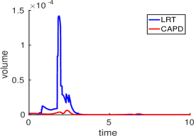
(a) horizon = $[0,10]$

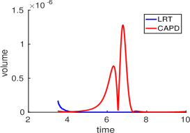
(b) horizon = $[3.5,10]$

Figure 4: Volume comparison for forced Van der Pol Oscillator

Some interesting observations about our experiments are as follows. Fig. 4 illustrates that the volumes of the LRT reachtube of the forced Van der Pol oscillator increase significantly for some initial time-steps compared to CAPD reachtube (nevertheless reduce in the long run). This initial increase is related to the computation of new coordinates, which are significantly different from the previous coordinates, resulting in a large stretching factor in step 7 of the LRT algorithm. Namely, we observed that it happens when the coordinates are switched from Case II to Case I, as presented in Section 3.6. We, however, observe that this does not happen in the system like MS cardiac model (see Fig. 5(a)). We believe those large increases of stretching factors in systems like fVDP can be avoided by smarter choices of the norms. We will further investigate those possibilities in future work.

Table 1 shows that LRT does not perform well for Lorentz attractor compared to CAPD (see also Fig. 5(b)), as the CAPD tool is current state of the art for such chaotic systems. LRT, however, performs much better than Flow* for this example. In all other examples, the LRT algorithm behaves favorably (outputs tighter reachtube, compare (F/I)V) in the long run.

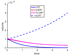
(a) Cardiac Model

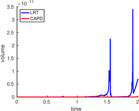
(b) Lorentz Attractor (Volumes computed by Flow* and nLRT are too large)

Figure 5: Volume comparison in two important benchmarks

5 Conclusions

We presented LRT, a rigorous procedure for computing ReachTube overapproximations based on Cauchy-Green stretching factor computation, in Lagrangian coordinates. We plan to pursue further research on our algorithm. One appealing possibility is to extend LRT to hybrid systems widely used in research on cardiac dynamics, and many other fields of study.

We also plan to implement LRT with forward-in-time integration and conservative-enclosures computation of the gradient, by just using a simple independent code (instead of CAPD). By such a code we mean a rigorous integration procedure based, for example, on the Taylor’s method. This code would directly compute an interval enclosure for the Cauchy-Green deformation tensors in an appropriate metric space. It would then be interesting to compare the wrapping-reduction performance of such a code with the procedure described above.

Acknowledgments

Research supported in part by the following grants: NSF IIS-1447549, NSF CPS-1446832, NSF CPS-1446725, NSF CNS-1445770, NSF CNS-1430010, AFOSR FA9550-14-1-0261 and ONR N00014-13-1-0090. J. Cyranka was supported in part by NSF grant DMS 1125174 and DARPA contract HR0011-16-2-0033.

Appendix 0.A Proofs of the Lemmas in Section 2

Lemma 3

Consider the Cauchy problem (1). Let $x_{0},y_{0}\in\mathbb{R}^{n}$ be two initial conditions at time $t_{0}$. Let $M\in\mathbb{R}^{n\times n}$ be a positive-definite symmetric matrix and $C^{T}C=M$ be its decomposition. For $t_{1}\geq t_{0}$, it holds that

$$\|\phi_{t_{0}}^{t_{1}}(x_{0}){-}\phi_{t_{0}}^{t_{1}}(y_{0})\|_{M}\,{\leq}\,\sqrt{\hat{\lambda}\left((C^{T})^{-1}\left(D_{x}\phi_{t_{0}}^{t_{1}}(\xi)\right)^{T}M\,D_{x}\phi_{t_{0}}^{t_{1}}(\xi)C^{-1}\right)}~{}\|x_{0}-y_{0}\|_{M}$$

where $\xi=\omega x_{0}+(1-\omega)y_{0}$ for some $\omega\in[0,1]$. For the particular case of the Euclidean norm, (8) takes the form

$$\|\phi_{t_{0}}^{t_{1}}(x_{0})-\phi_{t_{0}}^{t_{1}}(y_{0})\|_{2}\leq\sqrt{\lambda_{max}\left(\left(D_{x}\phi_{t_{0}}^{t_{1}}(\xi)\right)^{T}\cdot D_{x}\phi_{t_{0}}^{t_{1}}(\xi)\right)}~{}\|x_{0}-y_{0}\|_{2}.$$

Proof

Let $\xi(\omega)=\omega x_{0}+(1-\omega)y_{0}$. From

$$\int_{0}^{1}{D_{x}\phi_{t_{0}}^{t_{1}}(\xi(\omega))\,d\omega}=\frac{1}{x_{0}-y_{0}}\left(\phi_{t_{0}}^{t_{1}}(x_{0})-\phi_{t_{0}}^{t_{1}}(y_{0})\right),$$

and the well known mean value theorem for integrals, it holds that

$$\phi_{t_{0}}^{t_{1}}(x_{0})-\phi_{t_{0}}^{t_{1}}(y_{0})=D_{x}\phi_{t_{0}}^{t_{1}}(\hat{\xi})(x_{0}-y_{0})$$

for some $\hat{\omega}\in[0,1]$, $\xi(\hat{\omega})=\hat{\xi}$. From taking norms in above equation we obtain

$${\|\phi_{t_{0}}^{t_{1}}(x_{0})-\phi_{t_{0}}^{t_{1}}(y_{0})\|}=\|D_{x}\phi_{t_{0}}^{t_{1}}(\hat{\xi})(x_{0}-y_{0})\|\leq\|D_{x}\phi_{t_{0}}^{t_{1}}(\hat{\xi})\|\|x_{0}-y_{0}\|.$$

Replacing $\|D_{x}\phi_{t_{0}}^{t_{1}}(\hat{\xi})\|_{2}$ with the induced Euclidean matrix norm we obtain (9). If we use the weighted $M$-norm (6) we have for the matrix norm (7)

$$\|\phi_{t_{0}}^{t_{1}}(x_{0}){-}\phi_{t_{0}}^{t_{1}}(y_{0})\|_{M}\,{\leq}\,\sqrt{\lambda_{max}((C^{T})^{-1}\left(D_{x}\phi_{t_{0}}^{t_{1}}(\hat{\xi})\right)^{T}M\,D_{x}\phi_{t_{0}}^{t_{1}}(\hat{\xi})C^{-1})}~{}\|x_{0}-y_{0}\|_{M}$$

∎

Lemma 4

Consider the Cauchy problem (1). Let $x_{0},y_{0}\in\mathbb{R}^{n}$ be two initial conditions at time $t_{0}$. Let $M_{0},M_{1}\in\mathbb{R}^{n\times n}$ be positive-definite symmetric matrices, and $C_{0}^{T}C_{0}=M_{0}$, $C_{1}^{T}C_{1}=M_{1}$ their decompositions respectively. For $t_{1}\geq t_{0}$, it holds that

$$\|\phi_{t_{0}}^{t_{1}}(x_{0})-\phi_{t_{0}}^{t_{1}}(y_{0})\|_{M_{1}}\\ \leq\sqrt{\lambda_{max}\left((C_{0}^{T})^{-1}\cdot\left(D_{x}\phi_{t_{0}}^{t_{1}}(\xi)\right)^{T}\cdot M_{1}\cdot D_{x}\phi_{t_{0}}^{t_{1}}(\xi)\cdot C_{0}^{-1}\right)}~{}\|x_{0}-y_{0}\|_{M_{0}},$$

where $\xi=\omega x_{0}+(1-\omega)y_{0}$ for some $\omega\in[0,1]$.

Proof

Let $\xi=\omega x_{0}+(1-\omega)y_{0}$ for some $\omega\in[0,1]$. We use the equality $\phi_{t_{0}}^{t_{1}}(x_{0})-\phi_{t_{0}}^{t_{1}}(y_{0})=D_{x}\phi_{t_{0}}^{t_{1}}(\xi)(x_{0}-y_{0})$ derived in the proof of Lemma 1. Let us denote $A:=D_{x}\phi_{t_{0}}^{t_{1}}(\xi)$, and $w=(x_{0}-y_{0})$. It holds that

$$\|\phi_{t_{0}}^{t_{1}}(x_{0})-\phi_{t_{0}}^{t_{1}}(y_{0})\|_{M_{1}}=\|Aw\|_{M_{1}}=\sqrt{(Aw)^{T}M_{1}(Aw)}=\sqrt{w^{T}(A^{T}M_{1}A)w}=\\ \sqrt{w^{T}C_{0}^{T}((C_{0}^{T})^{-1}A^{T}M_{1}AC_{0}^{-1})C_{0}w}\leq\sqrt{\lambda_{max}\left((C_{0}^{T})^{-1}A^{T}M_{1}AC_{0}^{-1}\right)}\sqrt{w^{T}C_{0}^{T}C_{0}w}\\ =\sqrt{\lambda_{max}\left((C_{0}^{T})^{-1}A^{T}M_{1}AC_{0}^{-1}\right)}~{}\|w\|_{M_{0}}\quad\squareforqed$$

References

• [1] J. Anderson and A. Papachristodoulou. A decomposition technique for nonlinear dynamical system analysis. IEEE Transactions on Automatic Control, 57(6):1516–1521, 2012.
• [2] D. Angeli, E. D. Sontag, and Y. Wang. A characterization of integral input-to-state stability. IEEE Transactions on Automatic Control, 45(6):1082–1097, 2000.
• [3] M. Berz and K. Makino. Verified integration of odes and flows using differential algebraic methods on high-order taylor models. Reliable Computing, 4(4):361–369, 1998.
• [4] M. Capiński, J. Cyranka, Z. Galias, T. Kapela, M. Mrozek, P. Pilarczyk, D. Wilczak, P. Zgliczyński, and M. Żelawski. CAPD - computer assisted proofs in dynamics, a package for rigorous numerics, http://capd.ii.edu.pl/. Technical report, Jagiellonian University, Kraków, 2016.
• [5] X. Chen, E. Abraham, and S. Sankaranarayanan. Taylor model flowpipe construction for non-linear hybrid systems. In Proceedings of the 2012 IEEE 33rd Real-Time Systems Symposium, RTSS ’12, pages 183–192, Washington, DC, USA, 2012. IEEE Computer Society.
• [6] X. Chen, E. Ábrahám, and S. Sankaranarayanan. Flow*: An Analyzer for Non-linear Hybrid Systems, pages 258–263. Springer Berlin Heidelberg, Berlin, Heidelberg, 2013.
• [7] G. Dahlquist. Stability and Error Bounds in the Numerical Intgration of Ordinary Differential Equations. Transactions of the Royal Institute of Technology. Almqvist & Wiksells, Uppsala, 1958.
• [8] A. Donzé. Breach, A Toolbox for Verification and Parameter Synthesis of Hybrid Systems, pages 167–170. Springer Berlin Heidelberg, Berlin, Heidelberg, 2010.
• [9] A. Donzé and O. Maler. Systematic Simulation Using Sensitivity Analysis, pages 174–189. Springer Berlin Heidelberg, Berlin, Heidelberg, 2007.
• [10] C. Fan, J. Kapinski, X. Jin, and S. Mitra. Locally optimal reach set over-approximation for nonlinear systems. In Proceedings of the 13th International Conference on Embedded Software, EMSOFT ’16, pages 6:1–6:10, New York, NY, USA, 2016. ACM.
• [11] C. Fan and S. Mitra. Bounded Verification with On-the-Fly Discrepancy Computation, pages 446–463. Springer International Publishing, Cham, 2015.
• [12] Z. Galias and P. Zgliczyński. Computer assisted proof of chaos in the Lorenz equations. Physica D: Nonlinear Phenomena, 115(3):165 – 188, 1998.
• [13] K. Hashiguchi and Y. Yamakawa. Introduction to Finite Strain Theory for Continuum Elasto-Plasticity. Wiley Series in Computational Mechanics. Wiley, 2012.
• [14] M. A. Islam and J. Cyranka. LRT prototype implementation. http://www.cs.cmu.edu/~mdarifui/cav_codes.html, 2017.
• [15] T. Kapela and P. Zgliczyński. The existence of simple choreographies for the N-body problem—–a computer-assisted proof. Nonlinearity, 16(6):1899, 2003.
• [16] J. Lofberg. Yalmip: A toolbox for modeling and optimization in matlab. In Computer Aided Control Systems Design, 2004 IEEE International Symposium on, pages 284–289. IEEE, 2005.
• [17] W. Lohmiller and J.-J. E. Slotine. On contraction analysis for non-linear systems. Automatica, 34(6):683–696, June 1998.
• [18] E. N. Lorenz. Deterministic nonperiodic flow. Journal of the atmospheric sciences, 20(2):130–141, 1963.
• [19] S. M. Lozinskii. Error estimates for the numerical integration of ordinary differential equations, part i. Izv. Vyss. Uceb. Zaved. Matematica, 6:52–90, 1958.
• [20] J. Maidens and M. Arcak. Reachability analysis of nonlinear systems using matrix measures. IEEE Transactions on Automatic Control, 60(1):265–270, Jan 2015.
• [21] K. Makino and M. Berz. Cosy infinity version 9. Nuclear Instruments and Methods in Physics Research Section A: Accelerators, Spectrometers, Detectors and Associated Equipment, 558(1):346–350, 2006.
• [22] K. Makino and M. Berz. Rigorous integration of flows and odes using taylor models. Symbolic Numeric Computation, pages 79–84, 2009.
• [23] C. C. Mitchell and D. G. Schaeffer. A two-current model for the dynamics of cardiac membrane. Bulletin of mathematical biology, 65(5):767–793, 2003.
• [24] A. MOSEK. The mosek optimization tools version 3.2 (revision 8) user’s manual and reference, 2002.
• [25] N. S. Nedialkov. Interval tools for odes and daes. In 12th GAMM - IMACS International Symposium on Scientific Computing, Computer Arithmetic and Validated Numerics (SCAN 2006), pages 4–4, Sept 2006.
• [26] N. S. Nedialkov. Vnode-lp—a validated solver for initial value problems in ordinary differential equations. In Technical Report CAS-06-06-NN. 2006.
• [27] J. Rohn. Bounds on eigenvalues of interval matrices. ZAMM-Zeitschrift fur Angewandte Mathematik und Mechanik, 78(3):S1049, 1998.
• [28] J. Rohn. Versoft: Guide. Technical report, Technical Report, 2011.
• [29] S. Rump. Developments in Reliable Computing, chapter INTLAB - INTerval LABoratory, pages 77–104. Kluwer Academic Publishers, Dordrecht, 1999.
• [30] B. Van Der Pol. Vii. forced oscillations in a circuit with non-linear resistance.(reception with reactive triode). The London, Edinburgh, and Dublin Philosophical Magazine and Journal of Science, 3(13):65–80, 1927.
• [31] D. Wilczak and P. Zgliczyński. Heteroclinic connections between periodic orbits in planar restricted circular three body problem. Part ii. Communications in Mathematical Physics, 259(3):561–576, 2005.
• [32] D. Wilczak and P. Zgliczyński. $C^{r}$-Lohner algorithm. Schedae Informaticae, 2011(Volume 20), 2012.
• [33] P. Zgliczynski. $C^{1}$ Lohner Algorithm. Foundations of Computational Mathematics, 2(4):429–465, 2002.