Low energy constituent quark and pion effective couplings in a weak external magnetic field

Abstract

An effective model with pions and constituent quarks in the presence of a weak external background electromagnetic field is derived by starting from a dressed one gluon exchange quark-quark interaction. By applying the auxiliary field and background field methods, the structureless pion limit is considered to extract effective pion and constituent quark couplings in the presence of a weak magnetic field. The leading terms of a large quark and gluon masses expansion are obtained by resolving effective coupling constants which turn out to depend on a weak magnetic field. Two pion field definitions are considered for that. Several relations between the effective coupling constants and parameters can be derived exactly or in the limit of very large quark mass at zero and weak constant magnetic field. Among these ratios, the Gell Mann Oakes Renner and the quark level Goldberger Treiman relations are obtained. In addition to that, in the pion sector, the leading terms of Chiral Perturbation Theory coupled to the electromagnetic field is recovered. Some numerical estimates are provided for the effective coupling constants and parameters.

1 Introduction

The intrincated structure of Quantum Chromodynamics (QCD) makes very difficult the identification of the relation between its fundamental degrees of freedom and the models that describe quite well hadron and nuclear Physics in the vacuum and in a certain range of variables such as temperature, baryonic density, magnetic field and so on. Low energy effective models are usually based on phenomenology and also general theoretical results and symmetries from QCD. Effective field theory (EFT) have been developed and strengthened since the formulation of Chiral Perturbation Theory (ChPT) [1, 2, 3, 4] and they contribute for establishing these conceptual and calculational gaps between the two levels in the description of strong interactions systems. However they do not provide microscopic first ground numerical predictions for the low energy coefficients. First principles calculations provided by lattice QCD also contributes to these programs since they should offer the ultimate full theoretical numerical predictions. However it is also very interesting to establish sound relations between low energy effective models and EFT with QCD by deriving them from QCD. Different mechanisms have already been found to yield a large variety of effective couplings between hadrons, in particular quark-antiquark light mesons chiral dynamics have been investigated extensively with focus on reproducing the low energy coefficients of chiral perturbation theory with progressively improved account of QCD non Abelian effects, for example in Refs. [5, 6, 7, 8, 9, 10, 11, 12]. Quark-based models such as NJL [11] and constituent quark models [13, 14, 15] are some of the most successful ones describing a large variety of mesons and baryons observables and properties with least number of parameters. One of the most important ingredients of these models emerges from both the phenomenology of hadrons and also QCD: approximate chiral symmetry and its dynamical symmetry breaking (DChSB) [16]. The relevance of the chiral condensate as the order parameter for the DChSB is widely recognized in spite of some recent controverse about its location [17, 18, 19]. In this context, it was claimed that the chiral constituent quark model [13, 20] can give rise to a large Nc EFT that copes the large Nc expansion and the constituent quark model in Ref. [21]. This EFT is composed by the leading large $N_{c}$ terms for constituent quarks coupled to pions and constituent gluons, besides the leading terms of chiral perturbation theory. This EFT has been derived recently from a single leading term of the QCD effective action by considering quark polarization for a dressed (non perturbative) gluon exchange between quarks [12]. In the present work this derivation is addressed again with the coupling to a background electromagnetic field by considering one term of the QCD effective action that is the dressed one gluon exchange between quarks as discussed below.

Hadron dynamics in the presence of magnetic fields ($B_{0}$) have attracted the attention due to sizeable values in several systems such as in magnetars, $B_{0}\simeq 10^{15}$G, and non central relativistic heavy ions collisions (RHIC), $B_{0}\simeq 10^{18}$G, in spite of being formed for very short time interval [22]. Even such strong magnetic fields can be considered to be relatively small with respect to some hadron energy scales. For example, one may have a large constituent quark effective mass with respect to a weak magnetic field limit, and a small parameter such as $eB_{0}/{M^{*}}^{2}$ can be considered. For a constituent quark effective mass ${M^{*}}\simeq 0.31$GeV and $eB_{0}/{M^{*}}^{2}\sim 0.6$ it follows $eB_{0}\sim 0.06$GeV² or equivalently $eB_{0}\sim 3m_{\pi}^{2}$. By considering further that, with the magnetic catalysis the quark effective mass increases with the magnetic field, it might reach $M^{*}\sim 0.45$GeV for $B_{0}\sim 7m_{\pi}^{2}$, expected to appear in RHIC, the parameter of the expansion is $eB_{0}/{M^{*}}^{2}\sim 0.6$. This parameter is completely compatible with a weak electromagnetic background field such that: $|eA_{\mu}|<<M^{*}$ or $|eA_{\mu}|<M^{*}$. Many phenomena are expected to take place under finite magnetic field [23, 24, 25, 26, 27, 28, 29, 30, 31, 32, 33, 34, 35]. In particular it has been found that a magnetic field can yield modifications and corrections in the strength and type of the hadron interactions, in particular constituent quarks, gluons and pions [36, 37, 38, 39, 40, 41, 42].

The following low energy quark effective global color model [7, 8] coupled to a background electromagnetic field will be considered:

$$Z=N\int{\cal D}[\bar{\psi},\psi]\exp\;i\int_{x}\left[\bar{\psi}\left(i\not{D}-m\right)\psi-\frac{g^{2}}{2}\int_{y}j_{\mu}^{b}(x){\tilde{R}}^{\mu\nu}_{bc}(x-y)j_{\nu}^{c}(y)+\bar{\psi}J+J^{*}\psi\right],$$ (1)

where the color quark current is $j^{\mu}_{a}=\bar{\psi}\lambda_{a}\gamma^{\mu}\psi$, the sums in color, flavor and Dirac indices are implicit, $\int_{x}$ stands for $\int d^{4}x$, $a,b...=1,...(N_{c}^{2}-1)$ stand for color in the adjoint representation, and $i,j,k=0,1..$ will be used for SU(2) flavor indices, and the covariant quark derivative with the minimal coupling to the background photon is: $D_{\mu}=\partial_{\mu}-ieQA_{\mu}$ with the diagonal matrix $\hat{Q}=diag(2/3,-1/3)$. In several gauges the gluon kernel can be written in terms of the transversal and longitudinal components, $R_{T}(k)$ and $R_{L}(k)$, as:

$$\tilde{R}^{\mu\nu}_{ab}(k)=\delta_{ab}\left[\left(g^{\mu\nu}-\frac{k^{\mu}k^{\nu}}{k^{2}}\right)R_{T}(k)+\frac{k^{\mu}k^{\nu}}{k^{2}}R_{L}(k)\right].$$ (2)

Even if other terms arise from the non Abelian structure of the gluon sector, the quark-quark interaction (1) is a leading term of the QCD effective action. The use of a dressed (non perturbative) gluon propagator already takes into account non abelian contributions that garantees important effects. This approximation for the QCD effective action also is basically equivalent to the Schwinger Dyson equations at the rainbown ladder approximation [43]. Furthermore, it will be assumed and required that this dressed gluon propagator provides enough strength for DChSB as obtained for example in [43, 44, 45, 46, 47, 48, 49]. Although it is possible to include the contribution of further terms from the QCD effective action [10] the aim of this work is to identify and to compute the resulting pion and constituent quark interactions resulting from a one loop background field analysis for the interaction (1). Along this work the same method proposed in Ref. [12] will be considered with the use of the background field method to introduce the sea and constituent quarks and of the auxilary field method to introduce the light quark-antiquark chiral states and mesons. Vector currents associated to light vector mesons are neglected since they represent heavier states and mesons being less important at lower energies. Two different non linear definitions of the pion field are chosen by performing chiral rotations and they are exhibited in the Appendix A. Nevertheless all the steps of the calculation will be presented to incorporate the coupling to background photons. The resulting sea quark determinant is expanded for large quark and gluon masses.

Interactions of pions with constituent quarks within constituent quark models are expected to be equivalent to pion-nucleons couplings and our results reinforce this view. Firstly, effective couplings are written in terms of an external photon field that, in a second step, is reduced to a weak magnetic field $B_{0}$ that is incorporated into the effective coupling constants. Several exact or approximated ratios of the effective coupling constants and parameters are calculated. Among them, the Gell Mann Oakes Renner [50] and the Goldberger Treiman [51, 52] relations arise at zero or weak magnetic fields. Numerical estimates for the resulting effective coupling constants and parameters are presented in Section (5). In spite of the fact that the gluon propagator and the quark-gluon vertex may present magnetic field dependence as well these will not be considered. Since the gluon propagator is not really completely known two different gluon propagators are considered to provide numerical estimates. This work therefore extends the work presented in [12] by including the electromagnetic coupling of pions and constituent quarks. Some leading corrections to pion and constituent quark effective coupling constants due to weak magnetic field are also calculated in the logics of Ref. [41] where exclusively constituent quark effective self interactions had been considered. The pion sector has been investigated in similar and even more general calculations by considering their structure and by taking into account gluon 3-point and 4-point Green’s functions [7, 8, 10, 53]. The pion sector will be presented as a sort of benchmark to assure the procedure, within the limit of structureless mesons, reproduces all the leading terms of chiral perturbation theory even if the resulting expressions for the low energy coefficients do not contain all the structures from a more general calculation. The work is organized as follows. The background field method and the auxiliary field method are briefly reminded in Section (2). The two pion field definitions are presented shortly in the Appendix A and the equivalence between the leading pion and constituent couplings to the background photon of the two pion field definitions is shown in Appendix B. In section (3), the quark determinant is expanded in the leading order by choosing the pion field in the Weinberg’s definition in terms of covariant derivatives [54] and the effective coupling constants are resolved. Ratios between effective coupling constants are exhibited. In Section (4), the usual pion field in terms of exponential representation, $U,U^{\dagger}$, is considered for the expansion of the corresponding quark determinant. It yields, in the pion sector, Chiral Perturbation Theory coupled to the electromagnetic field. The constituent quark sector in the leading order yields the most relevant pion-quark effective couplings that are also calculated in the presence of the external electromagnetic field. Relations between the effective coupling constants are also exhibited at zero and weak magnetic field and numerical estimates are presented in Section (5). In the last Section there is a Summary.

2 Flavor structure and light mesons fields

A Fierz transformation [7, 8, 11] is performed for the interaction (1) and the color singlet terms are selected as usually. These non singlet color terms that are already smaller than the color singlet by a factor $1/N_{c}$. It will be shown just before Section (2.1) they yield only higher orders interaction terms being outside of the scope of the work. The Fierz transformation of the quark interaction above, denoted here by ${\cal F}(\Omega)=\Omega_{F}$, can be rewritten in terms of bilocal quark currents, $j_{i}^{q}(x,y)=\bar{\psi}(x)\Gamma^{q}\psi(y)$ where $q=s,p,v,a$ and $\Gamma_{s}=I_{2}.I_{4}$ (for the 2x2 flavor and 4x4 Dirac identities), $\Gamma_{p}=i\gamma_{5}\sigma_{i}$, $\Gamma_{v}^{\mu}=\gamma^{\mu}\sigma_{i}$ and $\Gamma_{a}^{\mu}=i\gamma_{5}\gamma^{\mu}\sigma_{i}$, where $\sigma_{i}$ are the flavor SU(2) Pauli matrices. The resulting non local interactions $\Omega_{F}$ are the following:

$$\Omega \equiv g^{2}j_{\mu}^{a}(x)\tilde{R}^{\mu\nu}_{ab}(x-y)j_{\nu}^{b}(y)$$ (3)

$$\Omega_{F} = 4\alpha g^{2}\left\{\left[j_{S}(x,y)j_{S}(y,x)+j_{P}^{i}(x,y)j_{P}^{i}(y,x)\right]R(x-y)\right.$$

$$- \left.\frac{1}{2}\left[j_{\mu}^{i}(x,y)j_{\nu}^{i}(y,x)+{j_{\mu}^{i}}_{A}(x,y){j_{\nu}^{i}}_{A}(y,x)\right]\bar{R}^{\mu\nu}(x-y)\right\},$$

where $i,j,k=0,...(N_{f}^{2}-1)$ and $4\alpha=8/9$ for SU(2) flavor. The kernels above can be written as:

$$R(x-y) \equiv 3R_{T}(x-y)+R_{L}(x-y),$$

$$\bar{R}^{\mu\nu}(x-y) \equiv g^{\mu\nu}(R_{T}(x-y)+R_{L}(x-y))+2\frac{\partial^{\mu}\partial^{\nu}}{\partial^{2}}(R_{T}(x-y)-R_{L}(x-y)).$$ (4)

A longwavelength local limit of expression (3) yields the Nambu Jona Lasinio (NJL) and vector NJL couplings.

By employing the background field method (BFM) [55, 16] it will be considered that quarks might either form light mesons and the chiral condensate or to be constituent quarks for baryons. So the quark field will be splitted into the (constituent quark) background field ($\psi_{1}$) and the sea quark field ($\psi_{2}$) that will be integrated out. For this, the following shift is performed: $\psi\to\psi_{1}+\psi_{2}$. This sort of decomposition is not exclusive to the BFM and it is found in other approaches [56]. The field $\psi_{2},\bar{\psi}_{2}$ will be integrated out and, for this, the action in (1) is expanded for the lowest one loop order as:

$$S\simeq S_{eff}[\bar{\psi}_{1},\psi_{1}]+\int\left({J}^{*}+\frac{\delta S_{eff}[\bar{\psi}_{1},\psi_{1}]}{\delta\psi_{1}}\right)\psi_{2}+\int\bar{\psi}_{2}\left(\frac{\delta S_{eff}[\bar{\psi}_{1},\psi_{1}]}{\delta\bar{\psi}_{1}}+J\right)+\int\bar{\psi}_{2}\frac{\delta S_{eff}[\bar{\psi}_{1},\psi_{1}]}{\delta\psi_{1}\delta\bar{\psi}_{1}}\psi_{2}+...,$$ (5)

where the first term is the tree level contribution and the linear terms are simply zero. Therefore at the one loop BFM level only the quadratic term contributes and it yield the same result as to perform the field splitting for the bilinears $\bar{\psi}\Gamma_{q}\psi$ [55]. It can be written that:

$$\bar{\psi}\Gamma^{q}\psi \to (\bar{\psi}\Gamma^{q}\psi)_{2}+(\bar{\psi}\Gamma^{q}\psi)_{1},$$ (6)

where $(\bar{\psi}\psi)_{2}$ will be treated in the usual way as valence quark of the NJL model. After a rearrangment the resulting full interaction $\Omega_{F}$ is splitted accordingly

$$\Omega_{F}\to\Omega_{1}+\Omega_{2}+\Omega_{12},$$

where $\Omega_{12}$ contains the interactions between the two components. This separation preserves chiral symmetry, and it might not be simply a mode separation of low and high energies. Besides that, the above shift of quark bilinears looks suitable for incorporating quark-anti-quark states which are the most relevant states for the low energy below the nucleon mass scale. To make possible to integrate out the component $\psi_{2}$, the interactions $\Omega_{2}$ can be handled in two ways:
(i) By considering a weak field approximation it can be neglected $\Omega_{2}<<\Omega_{1}$. This yields directly the one loop BFM that might receive corrections by a perturbative expansion which incorporates $\Omega_{2}$ [55];
(ii) By resorting to the auxiliary field method (AFM) with the introduction of a set of auxiliary fields by means of unitary functional integrals in the generating functional [7, 8, 12, 57]. A further advantadge of doing so is that the auxiliary fields (a.f.) allow to incorporate properly DChSB with the formation of the scalar quark condensate which endows quarks with a large effective mass. Therefore the second alternative improves the one loop BFM. Bilocal auxiliary fields ($S(x,y),P_{i}(x,y),V_{\mu}^{i}(x,y)$ and $\bar{A}_{\mu}^{i}(x,y)$) will be introduced by multiplying the generating functional by the following normalized Gaussian integrals:

$$1 = N\int D[S]D[P_{i}]e^{-\frac{i}{2}\int_{x,y}R\alpha\left[(S-gj^{S}_{(2)})^{2}+(P_{i}-gj^{P}_{i,(2)})^{2}\right]}\int D[V_{\mu}^{i}]e^{-\frac{i}{4}\int_{x,y}{\bar{R}^{\mu\nu}}\alpha\left[(V^{i}_{\mu}-gj_{V,\mu}^{i,(2)})(V^{i}_{\nu}-gj_{V,\nu}^{i,(2)})\right]}$$ (7)

$$\int D[\bar{A}_{\mu}^{i}]e^{-\frac{i}{4}\int_{x,y}{\bar{R}^{\mu\nu}}\alpha\left[(\bar{A}^{i}_{\mu}-g{j_{A,\mu}^{i,(2)}})(\bar{A}^{i}_{\nu}-g{j_{A,\nu}^{i,(2)}})\right]}.$$

The bilocal a.f. in this expression have been shifted by quark currents such as to cancel out the fourth order interactions $\Omega_{2}$. These shifts have unit Jacobian and they generate a.f. couplings to valence quarks. The procedure for the auxiliary field adopted in the present work for the meson sector follows the development proposed in Refs. [8, 7, 53]. This is discussed next by considering however the structureless mesons limit. Besides the meson sector however it contains bilinears of constituent quark field. They will compose interaction terms for baryons and mesons. The bilocal auxiliary fields can reduce to punctual meson fields by expanding in an infinite basis of local meson fields [8], for instance a particular bilocal field $\phi_{\alpha}(x,y)=S(x,y),P_{i}(x,y),V_{\mu}^{i}(x,y),\bar{A}_{\mu}^{i}(x,y)$ can be writtten in terms of a corresponding complete orhonormal sum of local fields $\xi_{\alpha}^{k}(u)$ as:

$$\phi_{\alpha}(x,y)=\Phi_{\alpha}\left(\frac{x+y}{2},x-y\right)=\Phi_{\alpha}(u,z)={F}_{\alpha}(z)+\sum_{k}F_{k,\alpha}(z)\xi_{\alpha}^{k}(u),$$ (8)

where $F_{\alpha},F_{k,\alpha}$ are vacuum functions invariant under translation for each of the bilocal mode and corresponding local field $\xi_{\alpha}^{k}(z)$ The low energy regime amounts to picking up only the low lying (lighest) modes $k=0$ and making the form factors to reduce to the zero momentum limit $F_{k,\alpha}(z)=F_{k,\alpha}(0)$, i.e. to constants. At the end the very long-wavelength limit can be reached by selecting the leading terms of these expansion which roughly correspond to simply considering the local limit for structureless lightest mesons. In this case $\xi_{\alpha}(u)=\xi_{\alpha}(x)$. This work is concerned with weak magnetic field effects in the low energy regime, the leading local field states of composite fields can be considered also the effects of magnetic field on the meson structure will be neglected. As a matter of fact, these effects should be relevant for much larger magnetic fields. Moreover, in the low energy regime the vector mesons should not be relevant to the dynamics since they are considerably heavier than the pion. In this limit, the above valence quark coupling to the local meson fields from expression (7), by omitting the index ₂, reduces to:

$$\bar{\psi}(x)\Xi(x,y)\psi(y)\simeq\bar{\psi}(x)F\left[s(x)+p_{i}(x)\gamma_{5}\sigma_{i}\right]\delta(x-y)\psi(y),$$ (9)

where $F$ is the pion decay constant that allows for the canonical definition of the pion field as $\pi_{i}=Fp_{i}$.

By considering the identity $\det A=\exp\;Tr\;\ln(A)$, the Gaussian integration of the valence quark field yields:

$$I_{det} = \;Tr\;\ln\;\left\{iS^{-1}(x-y)\right\}$$ (10)

where

$$S^{-1}(x-y) = {S_{0,c}}^{-1}(x-y)+\Xi(x-y)$$

$$+ 2R(x-y)\alpha g^{2}\left[(\bar{\psi}(y)\psi(x))+i\gamma_{5}\sigma_{i}(\bar{\psi}(y)i\gamma_{5}\sigma_{i}\psi(x))\right]$$

$$- \alpha g^{2}\bar{R}^{\mu\nu}(x-y)\gamma_{\mu}\sigma_{i}\left[\bar{\psi}(y)\gamma_{\nu}\sigma_{i}\psi(x)+i\gamma_{5}(\bar{\psi}(y)i\gamma_{5}\gamma_{\nu}\sigma_{i}\psi(x)\right],$$

where $Tr$ stands for traces of discrete internal indices and integration of spacetime coordinates, the quark kernel was defined as $S_{0,c}^{-1}(x-y)=\left(i\not{D}-m\right)\delta(x-y)$. In the absence of the external photon field $S_{0}^{-1}(x-y)=\left(i\not{\partial}-m\right)\delta(x-y)$. The above determinant has been already investigated in different limits. By neglecting the constituent quark field, it arises a low energy model in terms of low lying meson states [8, 53, 58]. By considering only the electromagnetic field, without mesons and quarks, an Euler-Heisenberg-type effective model emerges [59, 60, 61]. By considering only the constituent quark currents higher order quark effective interactions were obtained [62]. It was possible to trace back the symmetry breaking effective interactions to the quark mass and curiously these effective interactions were found to have strengths of the order of the chiral invariant effective interactions. Besides that, the conclusions from large Nc Witten analysis [63] were verified since the couplings behave as $N_{c}^{1-n}$ for $n$ quarks interactions. Finally pions and constituent quark currents have been considered for zero magnetic field in [12] and the resulting model turns out to be the large Nc effective field theory (EFT) proposed by Weinberg [21].

Now it is shown that the color non singlet terms neglected in expression (3) yield higher order contributions. Consider terms such as $1/N_{c}R(x-y)(\bar{\psi}\lambda_{\alpha}\psi)(\bar{\psi}\lambda_{\alpha}\psi)$ where $\lambda_{\alpha}$ are the Gell Mann color matrices. In the one loop BFM method their contribution in $\Omega_{2}$ are simply neglected [55]. The contribution of this term appears only in the integration of the quark field in expression (2) with extra terms of the type: $\Delta S^{-1}(x-y)=\lambda_{\alpha}R(x-y)g^{2}\bar{\psi}\lambda_{\alpha}\psi+...$ When performing the expansion of the determinant these terms only contribute in colorless combinations with extra factor $1/N_{c}$ for each quark current. Therefore they do not contribute to the leading pion and constituent quark sectors investigated in this work. If colorfull auxiliary fields $\tilde{S}_{\alpha}$ were introduced to make possible the integration of the corresponding term in $\Omega_{2}$, these fields would be not observables and they would have to be integrated out. These terms, after the use of the BFM as done above, would bring several corrections to the argument of the determinant (10) of the following type:

$$\Delta S^{-1}(x-y)=\lambda_{\alpha}\tilde{S}_{\alpha}+R(x-y)g^{2}\lambda_{\alpha}\bar{\psi}\lambda_{\alpha}\psi+...$$ (12)

With a saddle point expansion of the quark determinant there will have leading terms linear and quadratic $\tilde{S}_{\alpha}$ and $\tilde{S}_{\alpha}\tilde{S}_{\alpha}$. By integrating out these non observable colorfull auxiliary fields an additional determinant can be expanded again in a large quark mass limit for pions and constituent quark currents. This would yield extra terms that could be added to those terms found below in this work. These resulting contributions would have additional quark kernels $S_{0}(x-y)$ or, equivalently, extra factors $1/M^{*},1/{M^{*}}^{2}$ with respect to the terms of the expansion shown below. Therefore they are of higher order and numerically smaller in the large quark mass expansion. All these non leading terms however are outside the scope of the present work.

There is an ambiguity to define the pion field due to chiral invariance [64] and it is convenient to perform a chiral rotation to investigate only fluctuations around the ground state without the scalar field as a dynamical degree of freedom. In the Appendix A two different choices of the pion field are exhibited and they are used respectively in Sections (3) and (4) to investigate the quark determinant. In the first of them, for the chiral invariant terms the pion field always show up in terms of a covariant derivative ${\cal D}_{\mu}\vec{\pi}$. In the second and more usual definition, the exponential representation with functions $U,U^{\dagger}$ is chosen.

2.1 Gap equation

The a.f. were introduced without further considerations about their dynamics, in particular about their behavior in the ground state. To account for that, the saddle point equations for the effective action above (1) yield the usual gap equations. By denoting the auxiliary fields $\phi_{q}=S(x,y)$,$P_{i}(x,y)$, $V^{\mu}_{i}(x,y)$, $\bar{A}^{\mu}_{i}(x,y)$ these equations can be written as

$$\frac{\partial S_{eff}}{\partial\phi_{q}}=0.$$ (13)

These equations for the NJL model and GCM have been analyzed in many works for the vacuum, under external B, at finite temperatures or quark densities, including in the complete form which correspond to Dyson Schwinger equations in the rainbow ladder approximation. In the vacuum the only possible non trivial homogeneous solution might exist for the scalar field. The magnetic field is known to produce magnetic catalysis and it increases the resulting effective mass [26, 27, 24, 60]. In particular in Ref. [41] the same gap equation was solved for zero and weak magnetic field by considering an effective (and confining) non perturbative gluon propagator and some numerical values were exhibited. With the non zero expected value of the scalar field due to DChSB, the chiral rotation to the non linear realisations of chiral symmetry are usually performed and the dynamical field correspond to the fluctuations around the ground state which is described by the chiral condensate. This happens at the expense of defining a quark effective mass. The quark determinant (10) will therefore, from here on, be composed by the quark kernel given by:

$$S_{0,c}(x-y) \to S_{0,c}^{-1}(x-y)\equiv i\not{D}-M^{*},$$ (14)

where $M^{*}=m+\bar{S}$ where $m$ is the current quark mass and $\bar{S}$ the scalar quark condensate. When a particular gauge is choosen for $R$ and $\bar{R}$, the gauge fixing parameter can be determined by a condition of gauge independence such as: $\frac{\partial S_{eff}}{\partial\lambda}=0$. All the quantities in the effective action found below for quarks and pions, and also the gap equations above, depend basically on the gluon propagator and on the original QCD Lagrangian parameters: u-d current quark masses, gauge coupling $g$, a gauge fixing parameter $\lambda$.

To exhibit a numerical solution for the gap equation above, let us consider an effective longitudinal (confining) gluon propagator from [45, 65] form of: $g^{2}R^{\mu\nu}_{ab}(k)=K_{F}/(k^{2}+M_{g}^{2})^{2}g^{\mu\nu}\delta_{ab}$ where $K_{F}=8\pi^{3}M^{2}/9$, $g^{2}$ is the bare gauge coupling constant and $M_{G}^{2}$ an effective gluon mass [49, 43]. This effective propagator presents the strength of the zero momentum running coupling constant and a qualitative behavior of the deep infrared behavior. The gap equation, as well as all the expressions for the effective coupling constants derived below are finite, i.e. free of ultraviolet and infrared divergences. By considering $M_{g}=M\simeq 378$ MeV [45] and a current quark mass $m=10$MeV, it yields, for $B_{0}=0$, $s_{0}\simeq 210$ MeV for the scalar auxiliary field $s$ as defined, for which $M^{*}\simeq 220$ MeV. The dependence of the chiral condensate, and therefore the quark effective mass, on the constant magnetic field has been investigated extensively [24, 66, 67]. The increase of the density of states by accounting the lowest Landau levels with high degeneracy in this regime yields the increase of the chiral condensate. This so called magnetic catalysis has also been related to the positivity of the scalar QED $\beta-$ function [60]. The resulting effective quark mass dependence on the weak magnetic field was analysed in [41].

3 Large effective masses expansion for the Weinberg pion field

By performing the first chiral rotation as presented in the Appendix A, in expressions (94-95) for the so called Weinberg pion field definition, the quark determinant can be written (by omitting the dependence on spacetime coordinates) as:

$$S_{d} = C_{0}+\frac{i}{2}\;Tr\ln\left\{\left(1+{S}_{0,c}\left[\Phi_{W}+\left(\sum_{q}\bar{a}_{q}\Gamma_{q}j_{q}\right)\right]\right)^{*}\right.$$ (15)

$$\left.\left(1+S_{0,c}\left[\Phi_{W}+\left(\sum_{q}\bar{a}_{q}\Gamma_{q}j_{q}\right)\right]\right)\right\},$$

where the following quantities were defined:

$$\Phi_{W}=\Xi = \gamma^{\mu}\vec{\sigma}\cdot{\cal D}_{\mu}\vec{\pi}i\gamma_{5}+i\gamma^{\mu}\vec{\sigma}\cdot\frac{\vec{\pi}\times\partial_{\mu}\vec{\pi}}{1+{\vec{\pi}}^{2}}+4m\left(\frac{\vec{\pi}^{2}}{1+\vec{\pi}^{2}}-\frac{\epsilon_{ijk}\sigma_{k}\pi_{i}\pi_{j}}{1+\vec{\pi}^{2}}\right),$$ (16)

$$\sum_{q}a_{q}\Gamma_{q}j_{q}(x,y) = -K_{0}\bar{R}^{\mu\nu}(x-y)\gamma_{\mu}\sigma_{i}\left[(\bar{\psi}(y)\gamma_{\nu}\sigma_{i}\psi(x))+i\gamma_{5}(\bar{\psi}(y)i\gamma_{5}\gamma_{\nu}\sigma_{i}\psi(x))\right]$$ (17)

$$+ 2K_{0}R(x-y)\left[(\bar{\psi}(y)\psi(x))+i\gamma_{5}\sigma_{i}(\bar{\psi}(y)i\gamma_{5}\sigma_{i}\psi(x))\right],$$

$$C_{0} = \frac{i}{2}\;Tr\;\ln\bar{S}_{0,c}^{-1}S_{0,c},$$ (18)

where $K_{0}=\alpha g^{2}$ and $C_{0}$ contains corrections to the electromagnetic field effective action that will not be presented here and it reduces to a constant in the generating functional in the absence of the background photon field. The leading quark-pion and pion effective interactions in the absence of magnetic field correspond to the Weinberg large Nc EFT and they have already been obtained in [12]. Higher order terms of the expansion generate non leading contributions for the pion-quark couplings, however they can be seen to be suppressed by higher order powers of the kernel $S_{0}$ in the large quark mass limit. By neglecting the constituent quark currents this determinant has been investigated mainly for the large quark mass regime, or weak pion field, and more generally weak light mesons fields without the electromagnetic couplings in different works. The resulting leading terms shown below are written with coefficients (effective coupling constants) which contain momentum integrals with progressively higher powers of the quark and gluon kernels $S_{0}(k)$ and $R(k)$. The internal momentum structure of these terms, in the zero momentum exchange limit, can be written in general as $\int_{k}S_{0}^{n}(k)R^{m}(k)$ for $n=1,2,3..$ and $m=0,1,2...$ as presented in the next sections. Pion normalization constant is $F\simeq 92$MeV that is relatively small when compared to $M^{*}\simeq 200-300$MeV and therefore this expansion is compatible with the weak pion field expansion. These coefficients or effective coupling constants contain therefore momentum integrals $\int_{k}S_{0}^{n}(k)R^{m}(k)$ will be therefore progressively numerically smaller, already for quark and gluon effective masses of the order of 200-500 MeV. Therefore this action will be expanded for large quark and gluon effective masses and the strict convergence of this expansion will not be addressed in the present work.

3.1 First order terms

The expansion of the determinant yields non-local interaction terms and therefore form factors such as the following one:

$$I_{2}^{p} = i^{3}d_{1}2(\alpha g^{2})\;Tr\;\left[(({S}_{0}(x-z)S_{0}(z-y){\bar{R}^{\nu\rho}}(x-y)))\right.$$ (19)

$$\left.\gamma_{\mu}\gamma_{5}\sigma_{i}\gamma_{\nu}\gamma_{5}\sigma_{j}\epsilon_{imn}\frac{{\pi}_{m}(z)\partial^{\mu}{\pi}_{n}(z)}{1+\vec{\pi}^{2}(z)}(\bar{\psi}(y)\gamma_{\rho}\sigma_{j}\psi(x))\right],$$

where $d_{n}=i\frac{(-1)^{n+1}}{2n}$, the trace $Tr=tr_{C}\;tr_{F}\;tr_{D}\;tr_{k}$ is composed by the traces in all internal quantum numbers, color, flavor and Dirac indices, and spacetime with eventual momenta integration. However in the low energy limit one might resolve the traces above by considering zero momentum transfer between pions and constituent quarks. Therefore, by resolving the effective coupling constants in the corresponding local limit, the non zero first order leading effective quark-pion couplings and pameteres are given by:

$${\cal L}_{W}^{(1)} = g_{\chi 1}{\cal D}^{\mu}\vec{\pi}{\cal D}_{\mu}\vec{\pi}+i2g_{\pi v}\frac{\vec{\pi}\times\partial^{\nu}\vec{\pi}}{1+\vec{\pi}^{2}}\cdot(\bar{\psi}\gamma_{\nu}\vec{\sigma}\psi)+i2g_{\pi v}{\cal D}^{\nu}{\pi}^{i}\bar{\psi}i\gamma_{5}\gamma_{\nu}\sigma_{i}\psi,$$ (20)

$${\cal L}_{sb,1} = g_{sb1}(\bar{\psi}\psi)+g_{\beta sb1}F\left(\frac{\vec{\pi}^{2}}{1+\vec{\pi}^{2}}\right)(\bar{\psi}\psi)-g_{\beta psb}F^{2}\frac{\vec{\pi}^{2}}{1+\vec{\pi}^{2}}+g_{\chi sb}F^{4}\left(\frac{\vec{\pi}^{2}}{1+\vec{\pi}^{2}}\right)^{2},$$ (21)

where $F$ is the pion decay constant suitably introduced to provide the correct canonical definition of the pion field. In these expressions there are chiral invariant and symmetry breaking terms. The following effective coupling constants have been defined:

$$g_{\chi 1} = -iN_{c}d_{1}8\;Tr^{\prime}\;((\tilde{S}_{2}(k))),$$ (22)

$$g_{\pi v} = iN_{c}d_{1}4(\alpha g^{2})\;Tr^{\prime}\;((\tilde{S}_{2}(k)\bar{\bar{R}}(k))),$$ (23)

$$g_{sb1} = iN_{c}d_{1}16M^{*}(\alpha g^{2})\;Tr^{\prime}\;((\tilde{S}_{0}(k)R(k))),$$ (24)

$$g_{\beta sb1} = iN_{c}d_{1}64\frac{m}{F^{2}}(\alpha g^{2})\;Tr^{\prime}\;((\tilde{S}_{2}(k){R}(k)))$$ (25)

$$g_{\beta psb} = -iN_{c}d_{1}64\frac{M^{*}m}{F^{2}}\;Tr^{\prime}\;((\tilde{S}_{0}(k))),$$ (26)

$$g_{\chi sb} = iN_{c}d_{1}128\frac{m^{2}}{F^{4}}\;Tr^{\prime}\;((\tilde{S}_{2}(k))),$$ (27)

where the symbols $Tr^{\prime}\;((S_{m}(k)))$ indicates integration in momentum for combinations of the gluon kernel, $R(k)$ was written in expression (2), and the following functions for the local limit of the couplings:

$$\ \tilde{S}_{0}(k) = \frac{1}{k^{2}-M^{2}},$$ (28)

$$\tilde{S}_{2}(k) = \frac{k^{2}+M^{2}}{(k^{2}-M^{2})^{2}},$$ (29)

$$\bar{\bar{R}}(k) = g_{\mu\nu}\bar{R}^{\mu\nu}(k),$$ (30)

The first term in expression (20) $g_{\chi 1}$ reduces to the usual pion kinetic term with its coefficient the square pion decay constant $g_{\chi 1}=\frac{F^{2}_{\pi}}{2}$ [8, 12]. The effective constant $g_{\pi v}$ is the usual pion vector coupling constant which turns out to be equal to the axial coupling constant $g_{A}$. There are other terms of higher order in the pion field and they are not shown being also of higher order in the large $N_{c}$ limit.

The four terms in expression (21) are explicit symmetry breaking terms being their effective coupling constants proportional to the effective quark mass ( $M^{*}$) and to the current quark mass ($m$): $g_{sb1}$ is a correction to the constituent quark effetive mass, the second term ($g_{\beta sb1}$) corresponds to the sigma term effective coupling of pions to constituent quarks, and therefore to nucleons, the third term provides the Lagrangian mass to the pion $g_{\beta psb}=\frac{M_{\pi}^{2}}{2}.$ Expression (26) can be rewritten by considering the gap equation for the scalar auxiliary field $\bar{S}$ as to yield the Gell Mann Oakes Renner relation already presented in [12]:

$$\bar{S}\equiv<\bar{q}q> = -\frac{M_{\pi}^{2}}{m}F^{2},$$ (31)

where $M_{\pi}^{2}$ is proportional to $M^{*}$ according to expression (26). The last term $g_{\chi sb}$ contains the leading pion self interaction due to explicit symmetry breaking.

3.2 Leading couplings to the background photon

The leading effective couplings to photons are obtained by expanding the quark kernel. The next leading terms arise also from the second order terms of the quark determinant expansion that will not be presented here since they are smaller by a factor proportional to ${S}_{0}$ and therefore smaller by $1/{M^{*}}^{2}$. The leading corrections to the effective terms (20) in the very longwavelength and zero momentum transfer are the following:

$${\cal L}_{W}^{(1)} = ig_{\beta V}^{ij}F^{\mu\nu}\epsilon_{imn}\frac{{\pi}_{m}\times\partial_{\mu}{\pi}_{n}}{1+\vec{\pi}^{2}}(\bar{\psi}\gamma_{\nu}\sigma_{j}\psi)$$

$$+ ig_{\beta A}^{ij}F^{\mu\nu}{\cal D}_{\mu}{\pi}^{i}\bar{\psi}i\gamma_{5}\gamma_{\nu}\sigma_{j}\psi+g_{F\chi}^{ij}F^{\mu\nu}{\cal D}_{\mu}{\pi}_{i}{\cal D}_{\nu}{\pi}_{j},$$

where the effective coupling constants are given below. The coupling $g_{F\chi}$ provides an electromagnetic correction to the pion decay constant, the terms $g_{\beta V},g_{\beta A}$ provides a correction to the (constituent) quark vector and axial couplings to pions respectively.

The leading corrections to the leading chiral symmetry breaking couplings due to the background photon field are of higher order being given by:

$${\cal L}_{sb,1} = \left(g_{\beta sbF}F^{\mu\nu}F_{\mu\nu}+g_{\beta sbA}A_{\mu}A^{\mu}\right)\frac{\vec{\pi}^{2}}{1+\vec{\pi}^{2}}\bar{\psi}\psi$$

$$+ (g_{sb1F}F^{\mu\nu}F_{\mu\nu}+g_{sb1A}A_{\mu}A^{\mu})\bar{\psi}\psi$$

$$+ \left(g_{\beta psbF}F^{\mu\nu}F_{\mu\nu}+g_{\beta psbA}A_{\mu}A^{\mu}\right)\frac{\vec{\pi}^{2}}{1+\vec{\pi}^{2}}$$

$$+ \left(g_{\chi sbF}F^{\mu\nu}F_{\mu\nu}+g_{\chi sbA}A_{\mu}A^{\mu}\right)\left(\frac{\vec{\pi}^{2}}{1+\vec{\pi}^{2}}\right)^{2},$$

In this expression $g_{sb1F}$ and $g_{sb1A}$ provide electromagnetic correction to the constituent quark mass, whereas $g_{\beta psbA}$ and $g_{\beta psbF}$ for the pion mass. After taking the traces in Dirac and color indices, by separating the trace in flavor indices in the first expressions to explicitate its structure, the effective coupling constants in expressions (3.2,3.2) can be written as:

$$g_{\beta V}^{ij}=g_{\beta A}^{ij} = ieN_{c}d_{1}8(\alpha g^{2})\;tr_{F}(\left[\sigma_{i},Q\right]\sigma_{j})\;Tr^{\prime}\;((\tilde{S}_{2}(k)\tilde{S}_{0}(k)\bar{\bar{R}}(k))),$$ (34)

$$g_{F\chi}^{ij} = ieN_{c}d_{1}8\;tr_{F}(\left[Q,\sigma_{i}\right]\sigma_{j})\;Tr^{\prime}\;((\tilde{S}_{2}(k)\tilde{S}_{0}(k))),$$ (35)

$$g_{\beta sbF} = -ie^{2}N_{c}d_{1}\frac{80}{9}m(\alpha g^{2})\;Tr^{\prime}\;((\tilde{S}_{2}(k)\tilde{S}_{0}^{2}(k)\bar{\bar{R}}(k)))$$ (36)

$$g_{\beta sbA} = -ie^{2}N_{c}d_{1}\frac{80}{9}m(\alpha g^{2})\;Tr^{\prime}\;((\tilde{S}_{2}(k)\tilde{S}_{0}(k)R(k))),$$ (37)

$$g_{sb1F} = -ie^{2}N_{c}d_{1}\frac{40}{9}M^{*}(\alpha g^{2})\;Tr^{\prime}\;((\tilde{S}_{0}^{3}(k)R(k))),$$ (38)

$$g_{sb1A} = -ie^{2}N_{c}d_{1}\frac{40}{9}M^{*}(\alpha g^{2})\;Tr^{\prime}\;((\tilde{S}_{0}^{2}(k)R(k))),$$ (39)

$$g_{\beta psbF} = -ie^{2}N_{c}d_{1}\frac{160}{9}M^{*}m\;Tr^{\prime}\;((\tilde{S}_{0}^{3}(k))),$$ (40)

$$g_{\beta psbA} = -ie^{2}N_{c}d_{1}\frac{160}{9}M^{*}m\;Tr^{\prime}\;((\tilde{S}_{0}^{2}(k))),$$ (41)

$$g_{\chi sbA} = -ie^{2}N_{c}d_{1}\frac{128}{9}m^{2}\;Tr^{\prime}\;((\tilde{S}_{2}(k)\tilde{S}_{0}(k))),$$ (42)

$$g_{\chi sbF} = -ie^{2}N_{c}d_{1}\frac{128}{9}m^{2}\;Tr^{\prime}\;((\tilde{S}_{2}(k)\tilde{S}_{0}^{2}(k))).$$ (43)

Electromagnetic corrections to the chiral symmetry breaking terms shown in expression (3.2) also are all proportional to the current quark mass or effective valence quark mass. It can be noted that while the leading corrections to the chiral invariant effective couplings in the weak magnetic field regime correspond to the dipole magnetic couplings, being proportional to $F^{\mu\nu}$, the leading correctons to intrinsic symmetry breaking interactions are of higher order ($F_{\mu\nu}^{2}$ or $A_{\mu}^{2}$) and therefore they increase slower for weak magnetic field. Of course the interactions with the electromagnetic field break chiral and isospin symmetry.

In Figure 1, the diagrams corresponding to the expressions (3.2) for the weak electromanetic field coupling to the quark-pion effective interactions are exhibited. The dressed (non perturbative) gluon propagator is indicated by a wavy line with a full circle and pion represented by dashed lines. There are one photon (dotted line) couplings to the internal quark lines coupled to one and two pions in diagrams (1a) and (1b). The one pion coupling is the axial coupling and the two-pion coupling to quarks is the vector one. In diagrams (1c) and (1d) the corrections to the constituent quark mass are indicated.

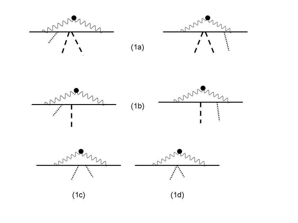
Figure 1: Diagrams (1a) and (1b) correspond to the quark-pion effective couplings from expression (3.2). The wavy line with a full dot is a (dressed) non perturbative gluon propagator, and the dotted and dashed lines represents respectively the background photon and pion fields, Diagrams (1c) and (1d) represent the quark mass corrections.

3.3 Ratios between effective coupling constants under finite magnetic field

Consider now a weak magnetic field in the Landau gauge by taking $A^{\mu}=B_{0}(0,-x,0,0)$, This magnetic field can be incorporated into the effective couplings shown in (34-43). The following terms with redefined effective coupling constants are obtained:

$${\cal L}_{W}^{(1)} = \textasciidieresis i\bar{g}_{\beta V}\epsilon_{ij3}\epsilon_{imn}\frac{{\pi}_{m}\times\partial_{x}{\pi}_{n}}{1+\vec{\pi}^{2}}(\bar{\psi}\gamma_{2}\sigma_{j}\psi)+i\bar{g}_{\beta A}\epsilon_{ij3}{\cal D}_{x}{\pi}^{i}\bar{\psi}i\gamma_{5}\gamma_{2}\sigma_{j}\psi+(\bar{g}_{sb1F}+\bar{g}_{sb1A})\bar{\psi}\psi$$ (44)

$$+ \bar{g}_{F\chi}\epsilon_{ij3}{\cal D}_{x}{\pi}_{i}{\cal D}_{y}{\pi}_{j}+\left(\bar{g}_{\beta sbF}+\bar{g}_{\beta sbA}\right)\frac{\vec{\pi}^{2}}{1+\vec{\pi}^{2}}\bar{\psi}\psi+\left(\bar{g}_{\beta psbF}+\bar{g}_{\beta psbA}\right)\frac{\vec{\pi}^{2}}{1+\vec{\pi}^{2}}$$

$$+ \left(\bar{g}_{\chi sbF}+\bar{g}_{\chi sbA}\right)\left(\frac{\vec{\pi}^{2}}{1+\vec{\pi}^{2}}\right)^{2},$$

where the effective coupling constants are:

$$\bar{g}_{\beta V}^{ij}=\bar{g}_{\beta A}^{ij} = B_{0}{g}_{\beta A}\epsilon_{ij3},$$ (45)

$$\bar{g}_{F\chi}^{ij} = B_{0}{g}_{F\chi}\epsilon_{ij3},$$ (46)

$$\bar{g}_{\beta sbF} = B_{0}g_{\beta sbF},$$ (47)

$$g_{\beta sbA} \simeq -ie^{2}B_{0}^{2}d_{1}\frac{80}{9}m(\alpha g^{2})\;Tr^{\prime}\;((\frac{\partial^{2}}{\partial q_{x}^{2}}[\tilde{S}_{2}(k)\tilde{S}(k)R(k)])),$$ (48)

$$\bar{g}_{sb1F} = B_{0}^{2}g_{sb1F},$$ (49)

$$\bar{g}_{sb1A} = -ie^{2}B_{0}^{2}d_{1}\frac{80}{9}m(\alpha g^{2})\;Tr^{\prime}\;((\frac{\partial^{2}}{\partial q_{x}^{2}}[\tilde{S}_{2}(k)\tilde{S}(k)R(k)])),$$ (50)

$$\bar{g}_{\beta psbF} = B_{0}^{2}g_{\beta psbF},$$ (51)

$$g_{\beta psbA} \simeq -ie^{2}B_{0}^{2}d_{1}M^{*}m\frac{320}{9}\;Tr^{\prime}\;((\frac{\partial^{2}}{\partial q_{x}^{2}}[\tilde{S}_{0}(k)\tilde{S}(k)])),$$ (52)

$$g_{\chi sbA} \simeq -ie^{2}B_{0}^{2}d_{1}\frac{128}{9}m^{2}\;Tr^{\prime}\;((\frac{\partial^{2}}{\partial q_{x}^{2}}[\tilde{S}_{2}(k)\tilde{S}(k)])),$$ (53)

$$\bar{g}_{\chi sbF} = B_{0}^{2}g_{\chi sbF}.$$ (54)

Some of the possible gauge invariant ratios between the $B$- dependent (45-54) and $B$- independent (22-27) effective coupling constants in the limit of very large quark effective mass are given by:

$$(i)\;\;\frac{\bar{g}_{\beta A}}{g_{\pi v}}\simeq\frac{eB_{0}}{{M^{*}}^{2}}, (ii)\;\;\frac{\bar{g}_{F\chi}}{g_{\chi 1}}\simeq\frac{eB_{0}}{{M^{*}}^{2}},$$

$$(iii)\;\;\frac{\bar{g}_{sb1F}}{g_{sb1}}\simeq\frac{5(eB_{0})^{2}}{9{M^{*}}^{4}}, (iv)\;\;\frac{\bar{g}_{\beta psbF}}{g_{\beta psb}}\simeq\frac{5(eB_{0})^{2}}{18{M^{*}}^{4}}.$$ (55)

The first and the second of these ratios indicate respectively the relative strength of the leading B-dependent correction for the axial coupling and of the pion decay constant with their values in the vacuum. The pion-constituent quark vector coupling constant presents the same expression as the axial coupling constant as shown above, and therefore the corresponding ratio is the same. They both yield contributions only for the charged pions due to the isospin tensor $\epsilon_{ij3}$. The second and third ratios are the leading B-dependent corrections to (chiral symmetry breaking) effective quark and pion masses being of higher order.

4 Large quark mass expansion for the second pion field - $U,U^{\dagger}$

Next let us consider the second pion field definition in terms of exponential functions $U$ and $U^{\dagger}$ presented in expression (97) of the Appendix. The quark determinant can be rewritten as:

$$I_{det} = \frac{1}{2}Tr\ln\left[\left(S_{0,c}^{-1}+\Xi+\sum_{q}a_{q}\Gamma_{q}j_{q}\right)\times\left({S}_{0,c}^{-1}+\Xi^{*}+\left(\sum_{q}\bar{a}_{q}\Gamma_{q}j_{q}\right)\right)^{*}\right],$$ (56)

where constituent quark bilinears were given in expression (17), being that $\bar{a}_{s}=-a_{s}$, $\bar{a}_{v}=-a_{v}$ and $\bar{a}_{p}=a_{p}$, $\bar{a}_{a}=a_{a}$. By neglecting quark bilinears and pion field this determinant yields a model of the type of the celebrated Euler Heisenberg effective action for for the electromagnetic field [59, 60, 61, 68]. Below, the leading quark-pion effective interactions and pion self interactions in the presence of the external photon field are presented. Most of the expressions in the absence of the photon field have been presented in [12]. However the pion coupling to the constituent quarks are exploited further below.

The action of the derivative operator and the background photon coupling (${\not{D}}$) on the terms for the pion field, $\Xi$, can be suitably written by making use of the following pion covariant derivative:

$$D_{\mu}U=\partial_{\mu}U+ieA_{\mu}\left[\frac{\tau_{3}}{2}\>,\;U\right],$$ (57)

$$(D_{\mu}U)^{\dagger}=\partial_{\mu}U^{\dagger}-ieA_{\mu}\left[\frac{\tau_{3}}{2}\>,\;U^{\dagger}\right],$$ (58)

where it was used that: $\left[Q\;,\;U\right]=\left[\frac{\tau_{3}}{2}\;,\;U\right]$.

The leading terms of this expansion will be calculated in the zero order derivative expansion. Besides that, only the leading terms in the pion field and in the pion derivative will be shown, i.e., terms of higher order in $(\pi_{i})^{m}$ (for $m>2$ or $4$) and $(\partial^{n}\vec{\pi})$ ($n\geq 2)$ will be neglected.

4.1 Leading and next leading pion and external photon couplings

The leading terms of the pion sector can be calculated to resolve the corresponding effective couplings constants which turn out to be the low energy coefficients (lec’s). These lec’s are written below in a different way than they were presented in [12]. By taking the traces of Dirac and color, the leading terms in the very longwavelength limit, by accounting the leading term from the expansion of the quark kernel for the bacground photon field coupling, are given by:

$${\cal L}_{1} = -g_{1}\;tr_{F}\;(U+U^{\dagger})+\frac{F^{2}}{4}g_{c}\;tr_{F}\;{D}^{\dagger}U^{\dagger}{D}U-l_{5}\;e^{2}\;tr_{F}\left(QF_{\mu\nu}U^{\dagger}QF^{\mu\nu}U\right),$$ (59)

where $tr_{F}$ stands for the trace in flavor indices and

$$g_{1} = -id_{1}4MFN_{c}\;Tr^{\prime}\;((\tilde{S}_{0}(k))),$$ (60)

$$g_{c}g_{\mu\nu} = id_{1}16g_{\mu\nu}N_{c}\;Tr^{\prime}\;((\tilde{S}_{0}^{2}(k))),$$ (61)

$$l_{5} = -id_{1}2F^{2}N_{c}\;Tr^{\prime}\;((\tilde{S}_{2}(k)\tilde{S}_{0}^{2}(k))).$$ (62)

In expression (59), the term $g_{1}$ is the usual leading symmetry breaking term that yields the pion mass, so that it can be written: $g_{1}=\frac{M_{\pi}^{2}F^{2}}{4}$. With the help of the gap equation (13) this term reduces to the usual Gell Mann Oakes Renner (GOR) relation $M\bar{S}=M<\bar{q}q>=-F^{2}M_{\pi}^{2}$. The second term is the lowest order pion kinetic term with the correct coupling to photons [1, 69]. The expected numerical value for the corresponding parameter is $g_{c}=1$. The leading correction to the GOR for a weak magnetic field will be presented below. The last term $l_{5}$ is one of the leading chiral symmetry breaking terms with coupling to the electromagnetic field.

The leading second order terms are precisely those for the next leading part of chiral perturbation theory. Again, by resolving effective coupling constants (lec’s) for the limit of zero momentum transfer, they can be written as:

$$I_{\pi-A_{\mu}} = +\frac{(l_{3}+l_{4})}{16}m_{\pi}^{4}\;tr_{F}\;(U^{2}+{U^{\dagger}}^{2})+\frac{l_{4}}{8}m_{\pi}^{2}\;tr_{F}\;\left({D}_{\mu}U^{\dagger}{D}^{\mu}U\right)\;(U+U^{\dagger})$$ (63)

$$- \frac{l_{1}}{4}\;tr_{F}\;(D_{\mu}U^{\dagger}D^{\mu}U)^{2}-\frac{l_{2}}{4}\;tr_{F}\;(D_{\mu}U^{\dagger}D_{\nu}U)\cdot(D^{\mu}U^{\dagger}D^{\nu}U),$$

where factors with powers of the pion mass were introduced in $l_{3},l_{4}$ coefficients to compare with usual notation [3], and the following low energy constants have been defined in the presence of an electromagnetic field:

$$l_{1}=-\frac{l_{2}}{2} = id_{2}N_{c}F^{4}64\;Tr^{\prime}\;((\tilde{S}_{0,c}^{4}(k))),$$ (64)

$$(l_{3}+l_{4}) = -id_{1}N_{c}16\frac{F^{2}M^{2}}{m_{\pi}^{4}}\;Tr^{\prime}\;((\tilde{S}_{0,c}^{2}(k))),$$ (65)

$$l_{4} = i\frac{1}{m_{\pi}^{2}}d_{2}N_{c}4\times 12F^{3}M\;Tr^{\prime}\;((\tilde{S}_{0,c}^{3}(k))),$$ (66)

where

$$\tilde{S}_{0,c}(k) = \frac{1}{({k}^{2}-\Delta_{A}-{M}^{2})},$$ (67)

and $\Delta_{A}$ given by $\Delta_{A}=e^{2}\hat{Q}^{2}A_{\mu}A^{\mu}+\frac{ie}{2}\hat{Q}\sigma_{\mu\nu}F^{\mu\nu}$. In the second order of the determinant expansion there are higher order terms of chiral perturbation theory that are not presented here.

In the limit of $\Delta_{A}=0$ for the expressions above the effective couplings (63) reduce basically to the fourth order terms ChPT weakly coupled to the electromagnetic field with coefficients defined differently. By considering the full expressions for the lec’s dependence on the electromagnetic field there appear corrections for the case of strong electromagnetic field, i.e. electromagnetic field dependent low energy constants. These corrections due to electromagnetic field can also be written in the usual way by expanding $\tilde{S}_{0,c}$ for weak electromagnetic field and this second procedure yields higher order terms of $B_{0}$-dependent ChPT.

There is another leading electromagnetic coupling to pions that arise from expanding the the low energy coefficient $g_{c}$ for weak electromagnetic field (61). By resolving the effective coupling by taking the traces in color and Dirac indices, it can be written as

$${\cal L}_{D-F} = -i\frac{l_{6}}{2}tr_{F}\left[\left(QF_{\mu\nu}(D^{\mu}U)^{\dagger}(D^{\nu}U)\right)+\left(QF_{\mu\nu}(D^{\mu}U)(D^{\nu}U)^{\dagger}\right)\right],$$ (68)

where

$$l_{6} = id_{1}e4N_{c}F^{2}\;Tr^{\prime}\;((\tilde{S}_{0}^{3}(k))).$$ (69)

This completes the leading terms of ChPT in the presence of a weak electromagnetic field [69, 1]. This structureless pion limit corresponds to a truncated version of more general calculations [8, 10] and the resulting leading terms of Chiral Perturbation Theory are the correct ones.

4.2 First order constituent quark-pion effective couplings

The leading effective constituent quark-pion terms arise in the very longwavelength limit are the following:

$${\cal L}_{q-\pi} = M_{3}\;j_{s}+g_{2js}F\;tr_{F}\;Z_{+}j_{s}+g_{ps}F\;tr_{F}(\sigma_{i}Z_{-})j_{ps}^{i}+i2g_{V}\;tr_{F}(\sigma_{i}\partial_{\mu}Z_{+})j^{V,\mu}_{i}$$ (70)

$$+ i2g_{A}\;tr_{F}(\sigma_{i}\partial_{\mu}Z_{-})j_{A,\mu}^{i},$$

where $Z_{\pm}=\frac{1}{2}(U\pm U^{\dagger})$ and where the following effective coupling constants were defined by calculating the traces in Dirac and color indices:

$$M_{3} = id_{1}16N_{c}{M^{*}}(\alpha g^{2})\;Tr^{\prime}\;((R(k)\tilde{S}_{0}(k))),$$ (71)

$$g_{2js}=-g_{ps} = id_{1}32N_{c}(\alpha g^{2})\;Tr^{\prime}\;((R(k)\tilde{S}_{2}(k))),$$ (72)

$$g_{V}=g_{A} = -id_{1}8M^{*}FN_{c}(\alpha g^{2})\;Tr^{\prime}\;((\bar{\bar{R}}(k)\tilde{S}_{0}^{2}(k))),$$ (73)

where the functions $\tilde{S}_{0}(k)$ and $\tilde{S}_{2}(k)$ were defined in (28-29), and $R(k)$, $\bar{\bar{R}}(k)$ were defined previously as well. The first term is a correction to the constituent quark mass, that is not necessarily the same as the effective mass from the gap equation [70], $g_{2js}$ yields a scalar coupling of two pions to a scalar quark current, the term $g_{ps}$ is the usual leading pseudoscalar pion coupling to quarks, $g_{V}$ the two pion coupling to a vector quark current and the last one is the usual $g_{A}$ the axial coupling. For the chiral sector defined by the Weinberg pion definition given in the previous Section, only the last two effective derivative couplings appear. For the correct canonical normalization of the pion field multiplicative factors $1/F$ must redefine the effective coupling constants.

4.3 Relations among pion-quark effective couplings

Although numerical estimations of these effective coupling constants are strongly dependent on the gluon propagator and on the value for the quark-gluon coupling constant, it is possible to obtain an estimation of their relative strength by considering their ratios in the large quark mass limit. It is interesting to note that the functions $R(k)$ and $\bar{\bar{R}}(k)$ obtained from the gluon kernels are related by $\bar{\bar{R}}(k)=2R(k)$. To mantain the standard dimensionless coupling constants, the axial and vector couplings must be divided by $F$ to cope with the canonical pion definition. Some ratios between the effective coupling constants are exact and others can be obtained for the limit of very large quark effective mass. By denoting $g_{A}^{\prime}$ and $g_{V}^{\prime}$ the dimensionless definition of the effective couplings, the following exact and approximated ratios between the effective coupling constants were obtained:

$$(i)\;\;\frac{g_{ps}}{g_{2js}} = -1,,\;\;\;\;\;\;\;\;(ii)\;\;\frac{g_{A}^{\prime}}{g_{V}^{\prime}}=1,$$ (74)

$$(iii)\;\;\frac{g_{ps}}{g_{A}^{\prime}} \sim \frac{M^{*}}{F},\;\;\;\;\;\;\;\;(iv)\;\;\frac{g_{2js}}{g_{V}^{\prime}}\sim-\frac{M^{*}}{F}.$$ (75)

Note that the first two ratios, (i) and (ii), are exact and equal to one. The ratios (iii) and (iv) are approximated and valid in the limit of large quark masses. The ratio (iii) is the quark-level Goldberger Treiman relation [51, 52, 16], and the last ratio (iv) is a scalar-vector coupling relation analogous to the Goldberger Treiman relation. The ratios (i) and (ii) are gauge invariant.

4.4 Leading quark-pion couplings with external photon

The leading constituent quark-pion effective couplings to photons are obtained from the expansion of the kernel $S_{0c}$. The leading terms in the local limit are given by:

$${\cal L}_{q-\pi-A} = \left(M_{AA}A_{\mu}^{2}+M_{FF}F_{\mu\nu}F^{\mu\nu}\right)\;j_{s}+g_{vmd}A_{\mu}\;j^{\mu}_{i=3}$$

$$+ \left(g_{F-js-\pi}\;F\;F_{\mu\nu}^{2}+g_{A-js-\pi}\;F\;A_{\mu}^{2}\right)tr_{F}(\left\{Q,Z_{+}\right\}Q)j_{s}$$

$$+ i\left(g_{F-ps-\pi}\;F\;F_{\mu\nu}^{2}+g_{A-ps-\pi}\;F\;A_{\mu}^{2}\right)tr_{F}\left(\left[Q,Z_{-}\right]\left[Q,\sigma_{i}\right]\right)j_{ps}^{i}$$

$$+ ig_{jVA}\;F\;F^{\mu\nu}tr_{F}(\left\{\partial_{\mu}Z_{+},Q\right\}\sigma_{i}+\left[Q,\ \sigma_{i}\right]\partial_{\mu}Z_{+})j_{V,\nu}^{i}$$

$$+ ig_{jAA}\;F\;F^{\mu\nu}tr_{F}([Q,\partial_{\mu}Z_{-}]\sigma_{i}+\left\{Q,\sigma_{i}\right\}\partial_{\mu}Z_{-})j_{A,\nu}^{i}\;+\;{\cal O}(A_{\mu}^{2}),$$

where, by taking the traces in Dirac and color indices, and also flavor indices for the first terms ($M_{3AA},M_{FF}$ and $g_{vdm}$) the following effective parameters and coupling constants have been defined:

$$M_{AA} = ie^{2}d_{1}N_{c}{M^{*}}\frac{80}{9}(\alpha g^{2})\;Tr^{\prime}\;((R(k)\tilde{S}_{0}^{3}(k))),$$ (77)

$$M_{FF} = ie^{2}d_{1}N_{c}{M^{*}}\frac{160}{9}(\alpha g^{2})\;Tr^{\prime}\;((R(k)\tilde{S}_{0}^{4}(k))),$$ (78)

$$g_{vmd} = ied_{1}N_{c}8(\alpha g^{2})\;Tr^{\prime}\;((\bar{\bar{R}}(k)\tilde{S}_{0}(k))),$$ (79)

$$g_{F-ps-\pi}=-g_{F-js-\pi} = ie^{2}d_{1}N_{c}16(\alpha g^{2})\;Tr^{\prime}\;((R(k)\tilde{S}_{2}(k)\tilde{S}_{0}^{2}(k)+R(k)\tilde{S}_{0}^{3}(k))),$$ (80)

$$g_{A-ps-\pi}=-g_{A-js-\pi} = ie^{2}d_{1}N_{c}8(\alpha g^{2})\;Tr^{\prime}\;((\frac{\partial^{2}}{\partial q_{x}^{2}}(R(k)\tilde{S}_{2}(k)\tilde{S}_{0}(k)+R(k)\tilde{S}_{0}^{2}(k)))),$$ (81)

$$g_{jVA}=g_{jAA} = ied_{1}N_{c}{M^{*}}8(\alpha g^{2})\;Tr^{\prime}\;((\bar{\bar{R}}(k)\tilde{S}_{0}^{3}(k))),$$ (82)

The first two terms in expression (4.4) provide corrections to the constituent quark mas. While $M_{AA}$ arises as a first order expansion of the quark kernel $M_{FF}$ is obtained in the next order of this expansion, nevertheless both are of the same order in powers of $1/{M^{*}}$. The second term is a vector meson dominance term, and it will not be investigated further in this work. The couplings $g_{F-js-\pi}$ and $j_{F-ps-\pi}$ are corrections to the scalar and pseudoscalar pion-quark couplings due to the electromagnetic field and $g_{jVA}$ and $j_{jAA}$ are the corresponding corrections to the vector and axial pion coupling to quarks. The leading corrections to the axial and vector effective couplings are dipole couplings to the electromagnetic field, whereas the scalar and pseudoscalar are of higher order. The pion canonical normalization would introduce further factors $F$ in the expressions for the coupling constants above.

The one loop diagrams corresponding to the leading terms of expression (4.4) are shown in Figure 2. There are constituent quark-one pion couplings to one and two photons - (2b) (respectively axial and pseudoscalar couplings) - and constituent quark-two pion coupling to one or two external photons (respectively vector and scalar couplings) - (2a). The corrections to the constituent quark mass shown in (2c).

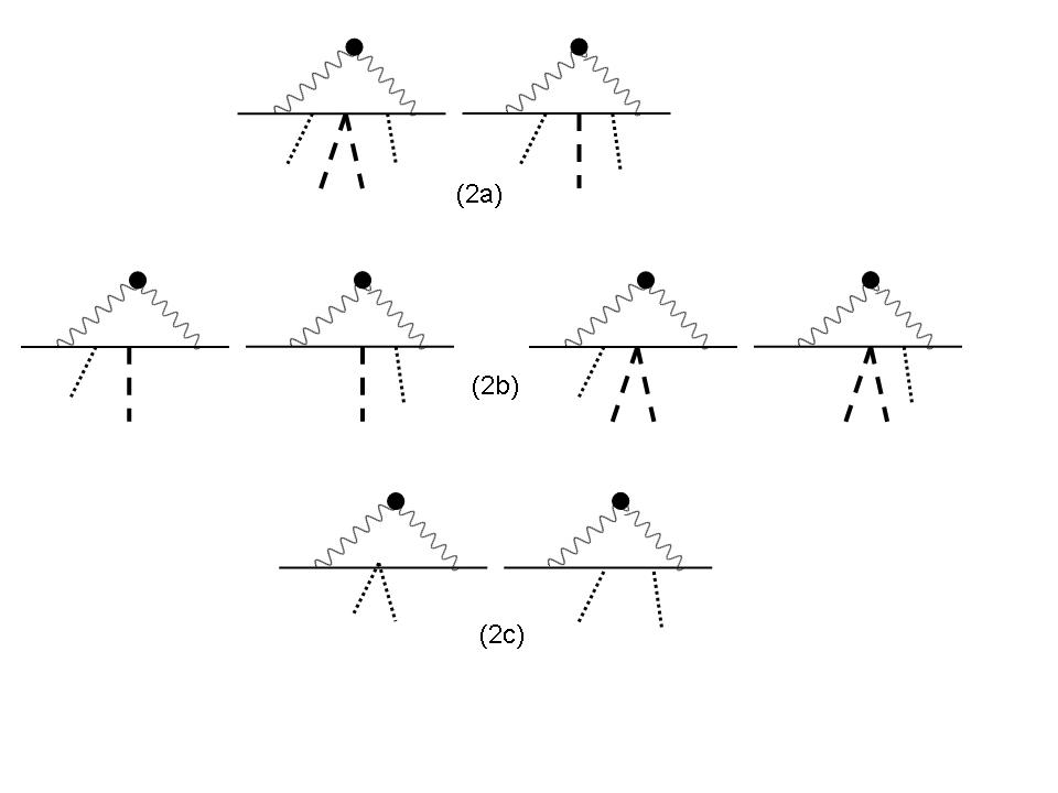
Figure 2: In these diagrams, the wavy line with a full dot is a (dressed) non perturbative gluon propagator, a dotted line represents the external photon field tensor $F^{\mu\nu}$, whereas the dashed line stands for the pion. Diagrams (2a) represent the scalar and pseudoscalar pion couplings to quarks (respectively two pions and one pion couplings) with further interaction to the photon field. Diagrams (2b) represents the axial and vector pion couplings to quarks (one and two pion couplings respectively) with a further one photon coupling In diagram (2c) the two contributions for the constituent quark effective mass due to the electromagnetic coupling.

4.5 Ratios between effective coupling constants under finite magnetic field

Let us show some approximated ratios in the same limit of large quark effective mass explored in Section (3.3) by fixing the same magnetic field $A^{\mu}=B_{0}(0,-x,0,0)$. From expression (4.4) the following $B_{0}$ dependent quark-pion effective couplings can be defined

$${\cal L}_{q-\pi-A} = \bar{M}_{B}\;j_{s}+\bar{g}_{Fjs\pi}\;tr_{F}(\left\{Q,Z_{+}\right\}Q)j_{s}+i\bar{g}_{Fps\pi}\;tr_{F}\left(\left\{Q,Z_{-}\right\}\left\{Q,\sigma_{i}\right\}\right)j_{ps}^{i}$$ (83)

$$+ i\bar{g}_{jVA}tr_{F}(\left[\partial_{x}Z_{+},Q\right]\sigma_{i})j_{V,y}^{i}+i\bar{g}_{jAA}tr_{F}([Q,\partial_{x}Z_{-}]\sigma_{i})j_{A,y}^{i},$$

where, by taking the traces in Dirac and color indices, and also flavor indices for the first three terms in (4.4) ($M_{AA},M_{FF},g_{vdm}$) and $\bar{M}_{B}$ the following effective coupling constants have been defined:

$$\bar{M}_{B} \simeq -i(eB_{0})^{2}d_{1}N_{c}{M^{*}}\frac{80}{9}Tr^{\prime}((R(k)\tilde{S}_{0}(k)\tilde{S}_{x}(k)+3R(k)\tilde{S}^{2}_{0}(k)\tilde{S}_{x}(k))),$$ (84)

$$\bar{g}_{Fjs\pi} = B_{0}^{2}\;g_{F-js-\pi},$$ (85)

$$\bar{g}_{Fps\pi} = B_{0}^{2}\;g_{F-ps-\pi},$$ (86)

$$\bar{g}_{jVA} = B_{0}\;{g}_{jVA},$$ (87)

$$\bar{g}_{jAA} = B_{0}\;g_{jAA}.$$ (88)

In the limit of large effective quark mass the following approximated ratios are obtained:

$$(i)\;\;\;\;\;\;\;\frac{M_{B}}{M_{3}}\sim\frac{5}{3}\frac{(eB_{0})^{2}}{{M^{*}}^{4}},\;\;\;\;\;\;\; (ii)\;\;\;\;\frac{\bar{g}_{Fjs\pi}}{g_{2js}}\sim\frac{5}{9}\frac{(eB_{0})^{2}}{{M^{*}}^{4}},\;\;\;\;\;\;\;\;\;\;$$ (89)

$$(iii)\;\;\;\frac{\bar{g}_{Fps\pi}}{g_{ps}}\sim\frac{10}{9}\frac{(eB_{0})^{2}}{{M^{*}}^{4}},\;\;\;\;\;\;\; (iv)\;\;\;\;\frac{\bar{g}_{jVA}}{g_{V}}=\frac{\bar{g}_{jAA}}{g_{A}}\sim 2\frac{eB_{0}}{{M^{*}}^{2}}.$$

These ratios show approximatedly the strength of the corrections for the effective couplings and effective mass due to the weak magnetic field. Ratios between B-dependent effective coupling constants from expression (83) can also be extracted, some of them are given by:

$$(i)\;\;\frac{\bar{g}_{Fjs\pi}}{\bar{g}_{Fps\pi}} \sim 2,\;\;\;\;\;\;\;\;\;\;\;\;\;\;\;\;\;\;(ii)\;\;\frac{\bar{g}_{jAA}}{\bar{g}_{jVA}}\sim 1,$$

$$(iii)\;\;\frac{\bar{g}_{Fps\pi}}{\bar{g}_{jAA}} \sim \frac{eB_{0}}{{M^{*}}^{2}}\frac{{M^{*}}}{F},\;\;\;\;\;(iv)\;\;\frac{\bar{g}_{Fjs\pi}}{\bar{g}_{jVA}}\sim\frac{eB_{0}}{{M^{*}}^{2}}\frac{M^{*}}{F}.$$ (90)

These expressions together with expressions (89) are $B_{0}$-dependent corrections to the relations (74) and (75).

5 Numerical estimates

Table 1: In the first column the chosen values for the quark effective mass are displayed with the corresponding UV cutoff $\Lambda_{i}$ and quark gluon coupling constant factor $h_{a}$. This factor was chosen to reproduce the value of the pion vector or axial coupling constant $g_{\pi v}=1$. In the second column the gluon propagator is indicated: $D_{I}$ and $D_{II}$ are the gluon propagators respectively from Refs. [43] and Ref. [45]. From the third to the last columns, values for the effective coupling constants from expressions (22,23,24,25,26,45,46,49,51) by considering the Weinberg pion field definition. Results from the expressions (45,46,49,51) divided by factor $(eB_{0})/{M^{*}}^{2}$ are displayed, being therefore independent of the magnetic field value. Values of the Euclidean cutoffs: $\Lambda_{1}=0.575$GeV, $\Lambda_{2}=0.433$GeV and $\Lambda_{3}=0.590$GeV. In the last line (exp. values) some experimental or expected values that reproduce experimental data. All the effective couplings or parameters that depend on the gluon propagator were multiplied by the same $h_{a}$ that corrects the strength of the quark gluon coupling constant.

$M^{*}$ ($\Lambda_{i}$, $h_{a}$)	$D_{i}(k)$	$f_{\pi}$	$g_{\pi v}h_{a}$	$g_{sb1}h_{a}$	$g_{\beta sb1}h_{a}$	$m_{\pi}$	$\frac{\bar{g}_{V}h_{a}}{(\frac{eB_{0}}{{M^{*}}^{2}})}$	$\frac{\bar{g}_{F\chi}}{(\frac{eB_{0}}{{M^{*}}^{2}})}$	$\frac{\bar{g}_{sb1F}h_{a}}{(\frac{eB_{0}}{{M^{*}}^{2}})}$	$\frac{m_{\pi}^{B}}{(\frac{eB_{0}}{{M^{*}}^{2}})}$
GeV (GeV, -)	-	(MeV)		(MeV)		(MeV)	-	(MeV)2	(MeV)	(MeV)
0.3   ($\Lambda_{1}$, $\frac{1}{3.4}$)	$D_{I}$	92	1	1470	2.3	218	0.8	0.1	111	56
0.3   ($\Lambda_{1}$, $\frac{1}{0.2}$)	$D_{II}$	92	1	3420	46	218	2.5	0.1	215	56
0.18   ($\Lambda_{2}$, $\frac{1}{12.8}$)	$D_{I}$	93	1	291	23	137	0.4	0.1	13	26
0.18   ($\Lambda_{2}$, $\frac{1}{0.7}$)	$D_{II}$	93	1	836	39	137	0.4	0.1	31	26
0.07   ($\Lambda_{3}$, $\frac{1}{32}$)	$D_{I}$	212	1	81	23	138	0.2	0.1	0.8	6.3
0.07   ($\Lambda_{3}$, $\frac{1}{1.8}$)	$D_{II}$	212	1	185	46	138	0.5	0.1	1.8	6.3
exp. values	-	92.4	1	313	-	140	-	-	-	-

In the Table 1 numerical values for some of the effective coupling constants and parameters of Section (3) are shown, in particular those exhibited in expressions (22,23,24,25,26,45,46,49,51). The integrations were carried out by performing an analytical continuation to Euclidean momentum space and few of them needed an ultraviolet cutoff. Two very different gluon propagators were chosen to make clear the ambiguity of the numerical estimates. The first of the gluon propagators, $D_{I}(k)$, is a transversal component from Tandy-Maris [43] and the second one, $D_{II}(k)$, is an effective longitudinal one by Cornwall that produces dynamical chiral symmetry breaking [45]. An ultraviolet cutoff was chosen for the integrals of the effective parameters $f_{\pi}$ and $m_{\pi}$, such that the at least one of their the experimental values is reproduced. Whenever possible, both $f_{\pi}$ and $m_{\pi}$ were fited with the same UV cutoff. Different values for the quark effective mass were considered. For the gluon propagator it was adopted the convention that

$$g^{2}\tilde{R}^{\mu\nu}(k)\;\equiv\;h_{a}D^{\mu\nu}_{i}(k),$$ (91)

where $D^{\mu\nu}_{i}(k)$ for $i=I,II$ and $h_{a}$ is a constant factor associated with the quark gluon coupling constant, and the reason for considering it is the following. All the effective parameters that depend on the gluon propagator and quark-gluon coupling constant were found to exhibit a systematic deviation from the known experimental values by nearly the same factor, whenever they have known experimental values. Therefore in the Table these effective coupling constants were multiplied by a factor $h_{a}$ indicated in the first column of the Table and it was chosen to reproduce the constituent quark-pion axial coupling constant $g_{\pi v}=1$ [21]. It corresponds to a particular choice of the quark gluon (running) coupling constant. The values that depend on the magnetic field, the effective couplings are divided by $(eB_{0})/{M^{*}}^{2}$ in such a way to become independent of the magnetic field. The resulting values listed in the last four columns of the Table must be multiplied by $\frac{(eB_{0})}{{M^{*}}^{2}}$ to be considered in expressions (45,46,49,51). The factor $\frac{(eB_{0})}{{M^{*}}^{2}}<<1$ or $\frac{(eB_{0})}{{M^{*}}^{2}}<1$ is the parameter for the weak magnetic field expansion. Therefore all the corrections induced by the weak magnetic field are small.

The numerical values for the estimates of expressions that do not depend on the gluon propagator are the following: $f_{\pi},m_{\pi},g_{F\chi}$ and $m_{\pi}^{B}$. The effective parameters $f_{\pi},m_{\pi}$ and the corresponding magnetic field dependent parameters $g_{F\chi},m_{\pi}^{B}$ could be expected to depend stronger in the pion structure which has been neglected when compared to the work presented in Ref. [8]. The resulting constituent quark effective mass $g_{sb1}$ might be too high and no apparent reason was identified, apart from the eventual excessively strong contribution from the gluon propagator and quark-gluon coupling. The quark effective mass and cutoff that best describe known experimental data in the Table are therefore $M^{*}=180$MeV and $\Lambda=433$MeV. For the last four columns there are not experimental values available.

In Table 2 some of the effective couplings and parameters found in Section (4) are exhibited, namely expressions (60,61,64,65,66,62,69,71,72,73) and also (84,86,87) . The same logics and input parameters used in Table 1 were considered. Again the factor $h_{a}$ in the identification (91) was chosen to produce the axial coupling constant to be $g_{v}=1$ [21]. The fact that pions were considered to be structureless, differently from Roberts and collaborators [8], imposes difficulties to reproducing the experimental values for $m_{\pi}=140$MeV and $g_{c}=1$. For the last three columns, where the coefficients for the magnetic field dependent corrections for effective coupling constants are shown, there are not experimental values available. The resulting values listed in the last four columns of the Table must be multiplied by $\left(\frac{(eB_{0})}{{M^{*}}^{2}}\right)^{n}$ for $n=1,2$. Therefore all the corrections induced by the weak magnetic field are very small. The definitions of the lec’s as written in expression (63) were chosen in agreement with Anderson [69], and the numerical values in the Table 2 were taken from Bijnens and Ecker [3]. The resulting numerical values are the one loop renormalized ones obtained from the following expression:

$$l_{i}^{r}=\frac{\gamma_{i}}{32\pi^{2}}\left(\bar{l}_{i}+\ln\frac{m_{\pi}^{2}}{\mu^{2}}\right),\;\;\;\;\mbox{ for $i=1,2,3,4,5,6$}.$$ (92)

being that all the numerical values of these parameters that reproduce experimental data were given in Refs. [3, 1]. Differently from results of the first pion field definition in Table 1, results from Table 2 indicate that the best choices for the quark effective mass and cutoff that reproduce better known experimental data are $M^{*}=70$MeV and $\Lambda=590$MeV. This value of the effecitve quark mass might be identified to a constituent quark mass for pions. The values for the parameter $g_{vmd}$ for the strength of the vector meson dominance effect are very small when comparing to the VMD coupling considered for example in Refs. [71].

Table 2: In the first column the following set of values are displayed $M^{*}$ for a given $\Lambda_{i}$, $D_{i}$ for the gluon propagator, $h_{a}$ is the quark gluon coupling constant factor. Two gluon propagators $D_{i}(k)=I$ or $II$ respectively from Refs. [43] and Ref. [45]. The sets of values are: (1) 0.3 GeV, I, $\frac{1}{2.6}$, (2) 0.3 GeV, II, $\frac{1}{0.3}$, (3) 0.18 GeV, I , $\frac{1}{4.1}$, (4) 0.18 GeV, II, $\frac{1}{0.5}$, (5) 0.07 GeV, I, $\frac{1}{5.9}$ and (6) 0.07 GeV, II, $\frac{1}{0.8}$. Values of the cutoffs: for $M^{*}=0.3$GeV $\Lambda_{1}=0.575$GeV, for $M^{*}=0.18$GeV $\Lambda_{2}=0.433$GeV and for $M^{*}=0.07$GeV $\Lambda_{3}=0.59$GeV. This factor was chosen to reproduce the value of the pion vector or axial coupling constant $g_{v}h_{a}=1$ and it multiplies the gluon propagator. From the second to the last columns, values for the effective coupling constants and parameters from expressions (60,61,64,65,66,62,69,71,72,73) and also (84,86,87) by considering the usual pion field definition in terms of the functions $U,U^{\dagger}$. Results from the expressions (84,86,87) divided by factors $(eB_{0})/{M^{*}}^{2}$ are displayed, being therefore independent of the magnetic field value. In the last line (e.v.) some experimental or expected values that reproduce experimental data. In this line the values of lec’s are extracted from Ref. [3] according to the definition written in the text.

sets	$m_{\pi}$	$g_{c}$	$l_{1}$	$l_{3}+l_{4}$	$l_{4}$	$l_{5}$	$l_{6}$	$M_{3}h_{a}$	$g_{ps}h_{a}$	$g_{v}h_{a}$	$\frac{\bar{M}_{B}h_{a}}{(\frac{eB_{0}}{{M^{*}}^{2}})^{2}}$	$\frac{\bar{g}_{ps}^{B}h_{a}}{(\frac{eB_{0}}{{M^{*}}^{2}})^{2}}$	$\frac{\bar{g}_{V}^{B}h_{a}}{(\frac{eB_{0}}{{M^{*}}^{2}})}$	$g_{vmd}h_{a}$
-	(MeV)	-	$10^{-4}$	$10^{-1}$	$10^{-2}$	$10^{-4}$	$10^{-3}$	(MeV)	-	-	(MeV)	-	-	(MeV)2
(1)	218	0.1	0.3	1.8	1.5	2.9	1.8	1752	2.6	1	628	1.8	1.1	0.2
(2)	218	0.1	0.3	1.8	1.5	2.9	1.8	1630	3	1	860	2.3	1.1	2.1
(3)	137	0.4	2	1.1	2.0	8.3	4.9	908	6.2	1	169	0.8	0.8	0.2
(4)	137	0.4	2	1.1	2.0	8.3	4.9	778	5.4	1	260	1.0	0.8	2.0
(5)	138	1.0	95	0.54	6.5	55	33	440	11	1	18.5	0.2	0.6	0.1
(6)	138	1.0	95	0.54	6.5	55	33	354	9	1	25	0.2	0.6	1.6
e.v.	140	1.0	88	0.6	6.8	55	31	313	13.5	1	-	-	-	-

6 Summary and final remarks

The leading magnetic field corrections to constituent quarks couplings to pions were found by considering one loop quark polarization for a dressed one gluon exchange quark interaction. For that, the quark field was separated into sea and constituent components by means of the background field method and the leading low energy quark-antiquark excitations were introduced by means of the auxiliary field method as it is usually done being that the lighest one, the pion field, was considered. The use of auxiliary fields contributes to an improvement of the one loop background field method by incorporating DChSB and the emergence of the scalar quark-antiquark condensate and then of the quark effective mass. The valence quark determinant was expanded for large quark and gluon effective masses by considering two different definitions of the pion field.

Firstly, the Weinberg’s pion field definition in terms of covariant pion and quark derivatives was used in Section (3). The leading terms of the quark determinant expansion turn out to be the constituent chiral quark model [20] in the version discussed in [21] that corresponds to a large $N_{c}$ EFT [12], with the corrections due to the interaction with the electromagnetic field. As discussed in Ref. [12] the relative ambiguity in separting the quark field into valence and constituent quark fields corresponds to the ambiguity of determining the relative contribution of constituent quarks sector and pions (or pion cloud) sector to describe hadron observables in the constituent chiral quark model [21, 72]. This issue deserves further investigation. Effective constituent quark-pion couplings were derived in the presence of the background photon field. Some ratios between the effective coupling constants for the limit of very large quark effective mass and weak magnetic field were found.

Secondly, the more usual pion field representation in terms of the exponential functions $U,U^{\dagger}$ was considered in Section (4). Concerning the coupling to the external electromagnetic field, the resulting leading terms in the pion sector correspond to the leading terms of Chiral Perturbation Theory coupled to photons which were found up to the fourth order in perfect agreement to the usual formulation [1, 3, 69]. It was shown however that some of the higher order photon-pion couplings in ChPT might be considered as electromagnetic corrections to some of the leading lec’s. Therefore it might be useful to consider ChPT calculations for stronger electromagnetic fields by considering $B_{0}$-corrections for the values of the lec’s. This pion field definition makes possible the emergence of different known pion effective couplings to quarks: vector, axial, pseudoscalar and scalar as shown in expressions (70,4.4). These expressions extend and complete previous work [12]. The corresponding couplings to the electromagnetic field explicitely break chiral and isospin symmetries, and they are relatively small with respect to the original pion-quark couplings because $\frac{(eB_{0})}{{M^{*}}^{2}}<1$ or $\frac{(eB_{0})}{{M^{*}}^{2}}<<1$. In this quark-pion sector the usual relevant effective couplings receive dipolar corrections of the order of $F_{\mu\nu}$ (vector and axial effective couplings) or higher order ones of the order of $F_{\mu\nu}^{2}$ and $A_{\mu}^{2}$ (scalar and pseudoscalar effective couplings). For larger magnetic fields the above expansion may be reliable by taking into account higher orders terms terms which produce effective interactions dependent on $[eB_{0}/{M^{*}}^{2}]^{n}$ for $n=1,2...$. The complete account of the Landau orbits [24, 66] appears to be equivalent to the resulting series in powers of the magnetic field, such as it has been done in this work, as shown explicitely in Ref. [73]. It is interesting to note that, in the leading order terms, the weak magnetic field does not mix the contribution of each of the gluon propagator components, transversal or longitudinal, for a particular effective coupling constant or parameter at this level of calculation.

Approximated and exact ratios between the effective couplings and parameters were extracted in the limit of large quark effective mass. They were exhibited in expressions (3.3,74,75,89,4.5), and they were found to yield expressions such as the emblematic Goldberger Treiman and GellMann Oakes Renner relations, besides new other relations with corresponding leading corrections due to weak electromagnetic (magnetic) field. Numerical estimations for the effective coupling constants and parameters were presented by choosing two very different gluon propagators from references [43] and [45]. The strength of the quark gluon coupling constant was normalized to produce the expected value for the vector pion coupling to constituent quarks that is equal to the axial coupling. Pion structure and gluon 3-point and 4-point Green’s functions do contribute for the resulting form factors, effective coupling constants and parameters [8, 9, 10] and these were not investigated in the present work. The magnetic field dependent coupling constants should be seen as partial contributions to the complete value because the gluon propagator and quark-gluon vertex also can present magnetic field dependent corrections that might be of same order of magnitude of the resulting effective coupling constants and parameters presented in this work.

Appendix A: Chiral rotations

By freezing the scalar field degree of freedom, chiral invariance yields the non linear representation. There is an ambiguity in defining the pion (and quark and all the fields respecting chiral symmetry) and different chiral rotations yield different pion field definitions [64, 16]. The quark free terms and its coupling to (scalar and pseudoscalar) chiral fields are given by:

$$\;\bar{\psi}_{2}\left[i\gamma\cdot\partial-m+\Phi_{L}\right]\psi_{2}=\;\bar{\psi}_{2}\left[i\gamma\cdot\partial-m+F(s+i\gamma_{5}\vec{\sigma}\cdot\vec{p})\right]\psi_{2}.$$ (93)

A possible redefinition of the quark and pion fields can be implemented by the following transformation [16, 54, 64]:

$$s=\frac{1-\vec{\pi}^{2}}{1+\vec{\pi}^{2}},\hskip 8.5359pt{p}_{i}=\frac{2\pi_{i}}{1+\vec{\pi}^{2}},\hskip 8.5359pt\psi = \frac{(1-i\gamma_{5}\vec{\sigma}\cdot\vec{\pi})}{\sqrt{1+\vec{\pi}^{2}}}\psi^{\prime}.$$ (94)

The above pion- quark coupling (93) can be rewritten as:

$$\bar{\psi}_{2}^{\prime}\left[i\gamma\cdot\partial-m^{*}+\gamma^{\mu}\vec{\sigma}\cdot\left(\frac{\partial_{\mu}\vec{\pi}}{1+\vec{\pi}^{2}}i\gamma_{5}+i\frac{\vec{\pi}\times\partial_{\mu}\vec{\pi}}{1+{\vec{\pi}}^{2}}\right)+4m\left(\frac{\vec{\pi}^{2}}{1+\vec{\pi}^{2}}-\frac{\epsilon_{ijk}\sigma_{k}\pi_{i}\pi_{j}}{1+\vec{\pi}^{2}}\right)\right]\psi_{2}^{\prime},$$ (95)

where it was used that $\sigma_{i}\sigma_{j}=\delta_{ij}+i\epsilon_{ijk}\sigma_{k}$. The last two terms in this expression correspond to the chiral symmetry breaking couplings in terms of the current quark mass. These terms yield some of the terms proportional to the pion mass or to powers of $\vec{\pi}^{2}$ in the resulting effective model. The following notation with two covariant derivatives is considered:

$${\cal D}_{\mu}\vec{\pi}\equiv\frac{\partial_{\mu}{\vec{\pi}}}{(1+\vec{\pi}^{2})},$$

$$\bar{\psi}_{2}\partial_{\mu}\psi_{2}\to\bar{\psi}_{2}^{\prime}D_{\mu}^{c}\psi_{2}^{\prime}\equiv\bar{\psi}_{2}^{\prime}\left(\partial_{\mu}+i\vec{\sigma}\cdot\frac{\vec{\pi}\times\partial_{\mu}\vec{\pi}}{1+{\vec{\pi}}^{2}}\right)\psi_{2}^{\prime}.$$ (96)

The canonically normalized pion field corresponds to $\vec{\pi}^{\prime}=\vec{\pi}F$ and the pion and valence quark fields will be denoted in the non linear realisation as: $\pi_{i}$ and $\psi_{2}$ respectively. This redefinition of the fields however induces a non trivial change in the functional measure with terms that do not depend on this pion covariant derivative. These terms will not be presented in this work.

A different parameterization of the non linear realization can be used for the pseudoscalar fluctuations around the vacuum to rewrite expression (93), as discussed in Refs. [8, 53], by means of :

$$\Phi_{L}\to\Phi_{NL} = F\left(P_{R}U+P_{L}U^{\dagger}\right),$$ (97)

where $U=e^{i\vec{\sigma}\cdot\vec{\pi}}$ and $P_{R,L}=(1\pm\gamma_{5})/2$ are the chirality projectors. These expressions allow to rewrite the pion sector in the standard form of Chiral Perturbation Theory.

Appendix B: Comparison between pion-quark couplings for the two pion definitions

For the comparison between the two pion field definitions for the low energy pion Physics regime, the weak pion field must be considered. For the two pion field definitions the following weak pion field expansions were considered:

$${\cal D}_{\mu}\vec{\pi} \simeq \partial_{\mu}\vec{\pi},\;\;\;\;\;\;\;\;\;\;\;\;\;\frac{1}{1+\vec{\pi}^{2}}\simeq 1+...$$ (98)

$$U \simeq 1+i\vec{\tau}\cdot\vec{\pi}+...,,\;\;\;\;\;\;U^{\dagger}\simeq 1-i\vec{\tau}\cdot\vec{\pi}+...$$ (99)

The traces in flavor indices of the Pauli matrices with the matrix $Q$ given after expression (1) were computed for most of the terms from expressions (20,21,3.2,3.2), from the Weinberg pion definition (W), and for expressions (70) and (4.4) from the second pion field definition (U). For the vector pion coupling with the electromagnetic coupling it has been used: $\epsilon_{ijk}\epsilon_{imn}=\delta_{jm}\delta_{kn}-\delta_{jn}\delta_{km}$. By using the same notation for both pion definitions, that again are written dimensionless $\vec{\pi}$, the pion-constituent quark couplings found in this work, with and without leading electromagnetic field coupling, can be written as:

$${\cal L}^{q-\pi}_{W} = 2g_{\pi v}\epsilon_{ijk}{\pi}_{i}(\partial^{\nu}{\pi}_{j})j_{V,\nu}^{k}+2g_{\pi v}({\partial}^{\nu}{\pi}^{i})j_{A,\nu}^{i}$$ (100)

$$+ g_{\beta sb1}F\vec{\pi}^{2}j_{s},$$ (101)

$${\cal L}^{q-\pi}_{W,B} = g_{\beta V}T_{jki}F^{\mu\nu}{\pi}_{j}\partial_{\mu}{\pi}_{k}j_{V,\nu}^{i}+g_{\beta A}\epsilon_{3ij}F^{\mu\nu}\partial_{\mu}{\pi}^{i}j_{A,\nu}^{j},$$ (102)

$$+ \left(g_{\beta sbF}{F^{\mu\nu}}^{2}+g_{\beta sbA}A_{\mu}A^{\mu}\right)\vec{\pi}^{2}j_{s}$$ (103)

$${\cal L}^{q-\pi}_{U} = g_{2js}F\;\vec{\pi}^{2}j_{s}+g_{ps}F{\pi}_{i}j_{ps}^{i}+i2g_{V}\epsilon_{ijk}\pi_{i}(\partial_{\mu}\pi_{j})j^{V,\mu}_{k}$$ (104)

$$+ 2g_{A}(\partial^{\mu}\pi_{i})j_{A,\mu}^{i},$$ (105)

$${\cal L}^{q-\pi}_{U,B} = -\left(g_{F-js-\pi}F_{\mu\nu}^{2}+g_{A-js-\pi}A_{\mu}A^{\mu}\right)F\frac{5}{9}\vec{\pi}^{2}j_{s}$$ (106)

$$- g_{F-ps-\pi}\;F\;F_{\mu\nu}^{2}\frac{4}{3}\epsilon_{ij3}\pi_{i}j_{ps}^{j},$$ (107)

$$- g_{jVA}\;F\;T_{jki}F^{\mu\nu}\frac{4}{3}\pi_{j}(\partial_{\mu}\pi_{k})j_{V,\nu}^{i}-g_{jAA}\;F\;F^{\mu\nu}\frac{4}{3}\epsilon_{ij3}\;\partial_{\mu}\pi_{i}\;j_{A,\nu}^{j},$$ (108)

where $T_{jki}=\delta_{ij}\delta_{3k}-\delta_{j3}\delta_{ik}$. The expressions ${\cal L}_{W}^{q-\pi}$ and ${\cal L}_{W,B}^{q-\pi}$ were extracted from eqs. (20,21,3.2,3.2) and the expressions ${\cal L}_{U}^{q-\pi}$ and ${\cal L}_{U,B}^{q-\pi}$ were calculated from eqs. (70,4.4). The couplings $g_{ps},g_{F-ps-\pi}$ only emerge in the pion definition in terms of functions $U,U^{\dagger}$. For the vector, axial and scalar couplings the following identification can be done:

$$g_{\pi v} \sim g_{V},\;\;\;\;\;\;\;\;\;\;\;\;\;g_{\pi v}\sim g_{A},$$

$$g_{\beta sb1} \sim g_{2js},\;\;\;\;\;\;\;\;\;\;\;g_{\beta V}\sim\frac{4F}{3}g_{jVA},$$

$$g_{\beta A} \sim \frac{4F}{3}g_{jVA},\;\;\;\;\;\;g_{\beta sbF}\sim\frac{5F}{9}g_{F-js-\pi},$$ (109)

$$g_{\beta sbA} \sim \frac{5F}{9}g_{A-js-\pi}.$$ (110)

Only the free pion terms were presented in both Sections 3.1 and 4.1 and they are trivially the same by a comparison of expressions (20,21) and (59).

References

- [1] J. Gasser, H. Leutwyler, Ann. Phys. (N.Y.) 158, 142 (1984).
- [2] S. Scherer, Eur. Phys. J. A 28, 59 (2006) S. Scherer, Prog. in Part. and Nucl. Phys. 64, 1 (2010).
- [3] J. Bijnens, G. Ecker, Annual Review of Nuclear and Particle Science 64, 149 (2014).
- [4] S. Weinberg, Physica A 96, 327 (1979).
- [5] Yu.A. Simonov, Phys. Rev. D 65, 094018 (2002).
- [6] A.A. Osipov, B. Hiller, and A.H. Blin, Eur. Phys. J. A 49, 14 (2013).
- [7] D. Ebert, H. Reinhardt, M.K. Volkov, Progr. Part. Nucl. Phys. 33, 1 (1994).
- [8] C.D. Roberts, R.T. Cahill, J. Praschifka, Ann. of Phys. 188, 20 (1988).
- [9] B. Holdom, Phys. Rev. D 45, 2534 (1992).
- [10] Q. Wang, Yu-P. Kuang, X-Lei Wang, M. Xiao, Phys. Rev. D 61, 054011 (2000). K. Ren, H-F. Fu, Q. Wang, Phys. Rev. D 95, 074012 (2017).
- [11] S.P. Klevansky, Rev. Mod. Phys. 64, 649 (1992). U. Vogl, W. Weise, Progr. in Part. and Nucl. Phys. 27, 195 (1991). T. Hatsuda, T. Kunihiro, Phys. Repts. 247, 1 (1994).
- [12] F.L. Braghin, Eur. Phys. Journ. A 52, 134 (2016).
- [13] E. de Rafael, Phys. Lett. B 703, 60 (2011).
- [14] M. Lavelle, D. McMullan, Phys. Rept. 279, 1 (1997).
- [15] A. W. Thomas, Nucl. Phys. B Proc. Suppl. 119, 50 (2003). R.D. Young, D.B. Leinweber, A.W. Thomas, Progr. in Part. and Nucl. Phys. 50 399 (2003), and references therein.
- [16] S. Weinberg, The Quantum Theory of Fields Vol. II, Cambridge, (1996).
- [17] S. J. Brodsky and R. Shrock, Phys. Lett. B 666, 95 (2008); arXiv:0803.2541.
- [18] S. J. Brodsky and R. Shrock, Proc. Natl. Acad. Sci. U.S.A. 108, 45 (2011); arXiv:0803.2554.
- [19] H. Reinhardt, H. Weigel, Phys. Rev. D 85, 074029 (2012).
- [20] A. Manohar and G. Georgi, Nucl. Phys. B 233, 232 (1984).
- [21] S. Weinberg, Phys. Rev. Lett. 105, 261601 (2010).
- [22] K. Tuchin, Advances in High Energy Physics 2013, 490495 (2013).
- [23] J. O. Andersen, W. R. Naylor, and A. Tranberg, Rev. Mod. Phys. 88, 025001 (2016); arXiv:1411.7176.
- [24] V. A. Miransky and I. A. Shovkovy, Phys. Rep. 576, 1 (2015).
- [25] V.A. Miransky, I.A. Shovkovy, Phys. Rev. D 66, 045006 (2002).
- [26] V.P. Gusynin, V.A. Miransky, I.A. Shovkovy, Nucl. Phys. B 462, 249 (1996).
- [27] G.S. Bali, F. Bruckmann, G. Endrodi, Z. Fodor, S.D. Katz, A. Schafer, Phys. Rev. D 86, 071502 (2012); arXiv:1206.4205.
- [28] K. Fukushima and Y. Hidaka, Phys. Rev. Lett. 110, 031601 (2013).
- [29] F. Bruckmann, G. Endrodi, and T. G. Kovacs, J. High Energy Phys. 04 112 (2013).
- [30] B. Chatterjee, H. Mishra, A. Mishra, Phys. Rev. D 91, 034031 (2015).
- [31] M.N. Chernodub, Phys. Rev. Lett. 106, 142003 (2011).
- [32] K. Fukushima, D. E. Kharzeev and H. J. Warringa, Phys. Rev. D 78, 074033 (2008); arXiv[hep-ph]:0808.3382.
- [33] D. E. Kharzeev, Prog. Part. Nucl. Phys. 75, 133 (2014). D. E. Kharzeev, Ann. Rev. Nucl. Part. Sci. 65, 193 (2015).
- [34] E.V. Gorbar, Phys.Lett. B 695, 354 (2011). For QED see Refs.: E.V. Gorbar, V.A. Miransky, I.A. Shovkovy, X. Wang, Phys. Rev. D 88, 025043 (2013). L. Xia, Phys. Rev. D 90, 085011 (2014)
- [35] J. Chao, P. Chu and M. Huang, Phys. Rev. D 88, 054009 (2013) arXiv:1305.1100 [hep-ph]. L. Yu, H. Liu and M. Huang, arXiv:1404.6969 [hep-ph].
- [36] E. J. Ferrer, V. de la Incera, and A. Sanchez, Phys. Rev. Lett. 107, 041602 (2011). E. J. Ferrer, V. de la Incera, and X. J. Wen, Phys. Rev. D 91, 054006 (2015). E. J. Ferrer et al, Rev. D 89, 085034 (2014).
- [37] R. L. S. Farias, K. P. Gomes, G. Krein, and M. B. Pinto, Phys. Rev. C 90, 025203 (2014).
- [38] A. Ayala, et al, arXiv:[hep-ph]1510.09134.
- [39] C.-F. Li, L. Yang, X.J. Wen, G.X. Peng, Phys. Rev. D 93, 054005 (2016)
- [40] M. A. Andreichikov, V. D. Orlovsky, and Y. A. Simonov, Phys. Rev. Lett. 110, 162002 (2013).
- [41] F.L. Braghin, Phys. Rev. D 94, 074030 (2016).
- [42] F.L. Braghin, Phys. Rev. D 97, 014022 (2018).
- [43] D. Binosi, L. Chang, J. Papavassiliou, C.D. Roberts, Phys. Lett. B 742, 183 (2015) and references therein.
- [44] K.-I. Kondo, Phys. Rev. D 57, 7467 (1998).
- [45] J.M. Cornwall, Phys. Rev. D 83 076001 (2011).
- [46] P. Maris, C. D. Roberts, Int. J. Mod. Phys. E 12 297 (2003). P. Tandy, Prog.Part.Nucl.Phys. 39 117 (1997).
- [47] K. Higashijima, Phys. Rev. D 29, 1228 (1984).
- [48] K.I. Aoki, et al., Prog. Theor. Phys. 84 683 (1990).
- [49] A. C. Aguilar, D. Binosi, J. Papavassiliou, Phys. Rev. D 84, 085026 (2011).
- [50] M. Gell-Mann, R.J. Oakes, B. Renner, Phys. Rev. 175, 2195 (1968).
- [51] M.L. Goldberger, S. Treiman, Phys. Rev. 111 , 354 (1966).
- [52] For example in: D. Barquilla-Cano, A. J. Buchmann, E. Hernndez, Nucl. Phys. A 714, 611 (2003); arXiv[nucl- th]0204067.
- [53] D. Ebert, H. Reinhardt, Nucl. Phys. B 271, 188 (1986).
- [54] S. Weinberg, Phys. Rev. 166, 1568 (1968).
- [55] L.F. Abbott, Acta Phys. Pol. B 13, 33 (1982). M.O.C. Gomes, Teoria Quântica de Campos, EDUSP, São Paulo, Brazil (2002).
- [56] F.L. Braghin, Phys. Rev. D 64 125001 (2001).
- [57] H. Kleinert, in Erice Summer Institute 1976, Understanding the Fundamental Constituents of Matter, 289, Plenum Press, New York, ed. by A. Zichichi (1978).
- [58] G. ’t Hooft, Nucl. Phys. B 72, 461 (1974).
- [59] W. Heisenberg, H. Euler, Z. Phys. 98, 714 (1936); translated into English: arxiv[physics]0605038.
- [60] G. S. Bali, et al , JHEP 2, 44 (2012); arXiv:1111.4956. G. Endrodi, JHEP 04 023 (2013); arXiv:1301.1307.
- [61] J. Schwinger, Phys. Rev. 82, (1951) 664; Phys. Rev. 93, (1953) 615.
- [62] F.L. Braghin, Phys. Lett. B 761, 424 (2016).
- [63] E. Witten, Nucl. Phys. B160, 57 (1979).
- [64] S. Weinberg, Phys. Rev. Lett. 18, 188 (1967).
- [65] For example in: J. Greensite, An Introduction to the Confinement Problem, Springer, Heildelberg (2011).
- [66] P. Watson, H. Reinhardt, Phys. Rev. D 89 045008 (2014).
- [67] G.S. Bali et al, J. High Energ. Phys. 04, 130 (2013).
- [68] C. Itzikson, J.-B. Zuber, Quantum Field Theory, McGraw Hill, (1985).
- [69] J.O. Andersen, JHEP 10, 005 (2012).
- [70] A. Paulo Jr, F.L. Braghin, Phys. Rev. D 90, 014049 (2014).
- [71] M. Benayoun, H.B. O’Connell, A.G. Williams, Phys.Rev. D 59 074020 (1999)
- [72] G. Kalbermann, Phys. Rev. D 33, 1987 (1986).
- [73] T.-K. Chyi, et al Phys. Rev. D 62, 105014 (2000).