A General Scheme Implicit Force Control for a Flexible-Link Manipulator

Abstract

In this paper we propose an implicit force control scheme for a one-link flexible manipulator that interact with a compliant environment. The controller was based in the mathematical model of the manipulator, considering the dynamics of the beam flexible and the gravitational force. With this method, the controller parameters are obtained from the structural parameters of the beam (link) of the manipulator. This controller ensure the stability based in the Lyapunov Theory. The controller proposed has two closed loops: the inner loop is a tracking control with gravitational force and vibration frequencies compensation and the outer loop is a implicit force control. To evaluate the performance of the controller, we have considered to three different manipulators (the length, the diameter were modified) and three environments with compliance modified. The results obtained from simulations verify the asymptotic tracking and regulated in position and force respectively and the vibrations suppression of the beam in a finite time.

1 Introduction

In the feedback control theory two types of controllers can be identified: unconstrained and constrained controllers. The unconstrained controller is used when the end-effector is not in contact with the environment, for example in robotics: feedback control for regulated and tracking control for position and velocity the end-effector respectively. The constrained controller is used when the end-effector is in contact with the environment, the force controller is classified inside constrained controller for robotics. The applications in control of force from manipulators have a combination of the two types of controllers, because is necessary first to localize the end-effector of the manipulator in the workspace in a point desired and then regulate to the force desired.
The following a review of the state of the art in force control. The hybrid controller proposed by Raibert & Craig in [1] and [2] is based on the workspace orthogonal decomposition in two subspaces: position control and force control. In [3] the system dynamics was included into the position-force controller. The impedance control by Hogan [4] combines both, position and force signals used in the complete manipulator-environment interaction. Such controllers can be used when the manipulator is in contact with the environment and also when it’s not in contact with the environment. The explicit force control [5] uses a force-error to regulated the closed loop. The implicit force control uses a tracking controller in stationary state to regulate the force applied to the environment.
In this paper we propose a scheme of Implicit Force Control for a one-link flexible manipulator, where the end-effector interacts with a compliant environment in the $x-y$ plane or vertical plane. The control scheme has two closed loop controllers. The inner loop is a tracking controller with gravity and vibration frequencies compensation. The outer loop is a implicit force controller. The scheme of force control this based on a dimensional finite mathematical model of the manipulator [6], [7]. This paper describes: 1) The mathematical model of the manipulator 2) The control scheme proposed 3) The stability analysis, 4) The results and analysis obtained and 5) Conclusions.

2 Mathematical model

The dynamics has been modelled in the joint space, where the system is the one-link flexible manipulator with rigid rotational joint. The gravitational force and the constrained environment are considered in this model.

2.1 Assumptions

The development mathematical model was based in the following assumptions:

1. The dynamics of the system has been obtained from the motion equation of Euler-Lagrange[8].

2. The links were modelled as a beam Euler-Bernoulli (EB)[9].

3. The transversal deformation was calculated in any point of the beam using the modes-assumed method.

4. The clamped-free beam as conditions of boundary of the beam.

$$M(\wp)\ddot{\wp}+C(\wp,\dot{\wp})\dot{\wp}+g(\wp)+\eta(\wp) = \tau-\tau_{e}$$ (1)

The equation of motion of the system when the manipulator is in contact with the environment is define by equation (1), where $M(\wp)$ the Inertia Matrix, $C(\wp,\dot{\wp})$ the Coriolis Matrix, $g(\wp)$ the gravitational force vector, $\eta(\wp)$ the vibrations frequency of the beam vector, $\tau$ torque vector and $\tau_{e}$ $\in$ $R^{nx1}$ the torque vector, caused by the environment as a reaction force when the end-effector apply a force on environment. The Fig. 1 show it the manipulator in contact with environment.

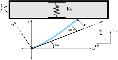
Figure 1: Flexible manipulator and compliant environment.

2.2 Equation

We show the mathematical expressions of the dynamic nonlinear model in spaces states of the manipulator. The equation (2), represents the evolution of the system in the time, from $L=\sum_{i}^{n}{K_{i}}-\sum_{i}^{n}{V_{i}}$, where $K_{i}$ is the kinetic energy for each link, $L_{i}$ is the potential energy for each link, and $\wp$ is the generalized coordinates of system corresponding to modes of vibrations of the beam. In this case $\wp=[\theta_{i}\quad q_{ij}]$, where $\theta_{i}$ is the rotation angle in the articulation and $q_{ij}$ is the generalized coordinate associated to temporal of modes or vibration frequencies, $i$ is the number associated of the link, $j$ is the number of modes of vibration flexible link, and $Q_{i}$ is the generalized force for each d.o.f of the system.

$$\frac{d}{dt}\Big{(}\frac{\partial L}{d\dot{\wp_{i}}}\Big{)}-\frac{\partial L}{\partial\wp_{i}}=Q_{i}$$ (2)

We have considered the planar position of the manipulator, the equation (7) define the position end-effector of the manipulator, considering the deformation of the beam in the end-effector. The kinetic energy are represent by equations (8) and (9), where: $A$, $\rho$, $I_{b}$ and $l$, are cross-sectional area, uniform mass density, inertia and length of link respectively of the beam (link).

$$P\left[\begin{array}[]{l}\hat{x}\\ y\\ \end{array}\right]^{T}=\left[\begin{array}[]{r}\hat{x}cos(\theta_{i}(t))-w_{i}(\hat{x},t)sin(\theta_{i}(t))\\ \hat{x}sin(\theta_{i}(t))+w_{i}(\hat{x},t)cos(\theta_{i}(t))\\ \end{array}\right]^{T}$$ (7)

$$K_{i}=\frac{1}{2}\int_{0}^{l_{1}}\dot{P}(\hat{x})^{T}\dot{P}(\hat{x})dm$$ (8)

$$K_{i}=\frac{1}{2}\dot{\theta}_{i}^{2}I_{bi}+\frac{1}{2}\rho_{i}A_{i}\dot{\theta}_{i}^{2}\int_{0}^{l_{i}}w_{i}^{2}(\hat{x},t)d\hat{x}+$$

$$\frac{1}{2}\rho_{i}A_{i}\int_{0}^{l_{i}}\dot{w}_{i}^{2}(\hat{x},t)d\hat{x}+\rho_{i}A_{i}\dot{\theta}_{i}\int_{0}^{l_{i}}\hat{x}\dot{w}_{i}(\hat{x},t)d\hat{x}$$ (9)

The potential energy (V) has two components, the component associated to the gravitational force ($V_{g}$) and the component associated to the beam deformation ($V_{e}$). The equations (10)-(2.2) represent the potencial energy of the system.

$$V=V_{g}+V_{e}$$ (10)

$$V_{g}=-\int_{0}^{l_{i}}g^{T}\textbf{P}dm$$ (11)

$$V_{e}=\frac{1}{2}EI\int_{0}^{l_{i}}[w_{i}^{"}(\hat{x},t)]^{2}d\hat{x}$$ (12)

$$V=\rho_{i}A_{i}g\frac{l_{1}^{2}}{2}sin(\theta_{i})+\rho_{i}A_{i}gcos(\theta_{i})\int_{0}^{l_{i}}w_{1}(\hat{x},t)d\hat{x}$$

$$+\frac{1}{2}EI\int_{0}^{l_{i}}[w_{i}^{"}(\hat{x},t)]^{2}d\hat{x}$$ (13)

From (9) and (2.2) and replace in (2) for one link i.e. $i=1$, and using the separability principle [10], for $w_{i}(\hat{x},t)$, the equation of motion might be obtained, furthermore expanded $w_{i}(\hat{x},t)=\sum_{j=1}^{\nu}\phi_{ij}(\hat{x})q_{ij}(t)$ for $2$ modes $(\nu=2)$, and representing the equation of the system by state variables (2.2), where $x$ is the state vector and expanding for describe variables $x=[\theta_{1}\quad\dot{\theta}_{1}\quad q_{11}\quad\dot{q}_{11}\quad q_{12}\quad\dot{q}_{12}]^{T}$, and the control vector $u=\tau-\tau_{e}$.

$$\dot{x}=f(x)+\varrho(x)u$$

$$y=h(x)$$ (14)

The equation (15), representing the mathematical model in state variables, where the constants was defined by: $b_{0}=a_{0}\rho_{1}A_{1}$, $b_{1}=\rho_{1}A_{1}\frac{a^{2}_{1}}{a_{0}}$, $b_{2}=\rho_{1}A_{1}a_{1}$, $b_{3}=\frac{a_{1}}{a_{0}}$ $b_{4}=\frac{l_{1}^{2}}{2}\rho_{1}A_{1}$, $b_{5}=a_{2}\rho_{1}A_{1}$ $b_{6}=EIa_{3}$, $b_{7}=\frac{a_{2}}{a_{0}}$ $b_{8}=I_{b1}$ and $a_{0}=\int_{0}^{l_{1}}\phi_{11}(\hat{x})^{2}d\hat{x}$, $a_{1}=\int_{0}^{l_{1}}\phi_{11}(\hat{x})\hat{x}d\hat{x}$, $a_{2}=\int_{0}^{l_{1}}\phi_{11}(\hat{x})d\hat{x}$, $a_{3}=\int_{0}^{l_{1}}\Big{[}\frac{d\phi_{11}^{2}{\hat{x}}}{d\hat{x}^{2}}\Big{]}^{2}d\hat{x}$, is important remarking that the equation (15) can be expanded for $n$ modes of vibrations, for details see [6].

$$\dot{x}_{1} = x_{2}$$

$$\dot{x}_{2} = \Big{[}\tau-x_{3}[2b_{01}x_{2}x_{4}+b_{21}(x^{2}_{2}+b_{71}gc_{1})-b_{31}b_{61}+{}$$

$${}b_{4}gc_{1}+b_{51}gs_{1}]-x_{5}[x_{2}(2b_{02}x_{6}+b_{22}x_{2})+{}$$

$${}b_{62}b_{32}+b_{52}gs_{1}]+b_{22}b_{72}gc_{1}\Big{]}\Big{[}b_{01}x^{2}_{3}+b_{11}+{}$$

$${}b_{02}x^{2}_{5}+b_{12}+b_{8}\Big{]}^{-1}$$

$$\dot{x}_{3} = x_{4}$$

$$\dot{x}_{4} = \Big{[}x^{2}_{2}x_{3}-b_{31}\dot{x}_{2}-b_{71}gc_{1}-\frac{b_{61}}{b_{01}}x_{3}\Big{]}$$

$$\dot{x}_{5} = x_{6}$$

$$\dot{x}_{6} = \Big{[}x^{2}_{2}x_{5}-b_{32}\dot{x}_{2}-b_{72}gc_{1}-\frac{b_{62}}{b_{02}}x_{5}\Big{]}$$ (15)

3 Control Scheme

We propose a control scheme with two closed-loop. The Fig. 2 show this scheme. The inner loop is a tracking control with gravity and vibration frequencies compensation. The outer loop is a force controller. The control scheme force transforms the force error into a position difference in the components planar $x$ and $y$. This difference is added to the reference of the tracking controller inner loop. The environment has been modelled as a deformable environment or compliant surface. When the manipulator makes contact with the environment a reaction force is generated $Fc=(Fc_{x},Fc_{y})$ and this components are feedback to the force controller.

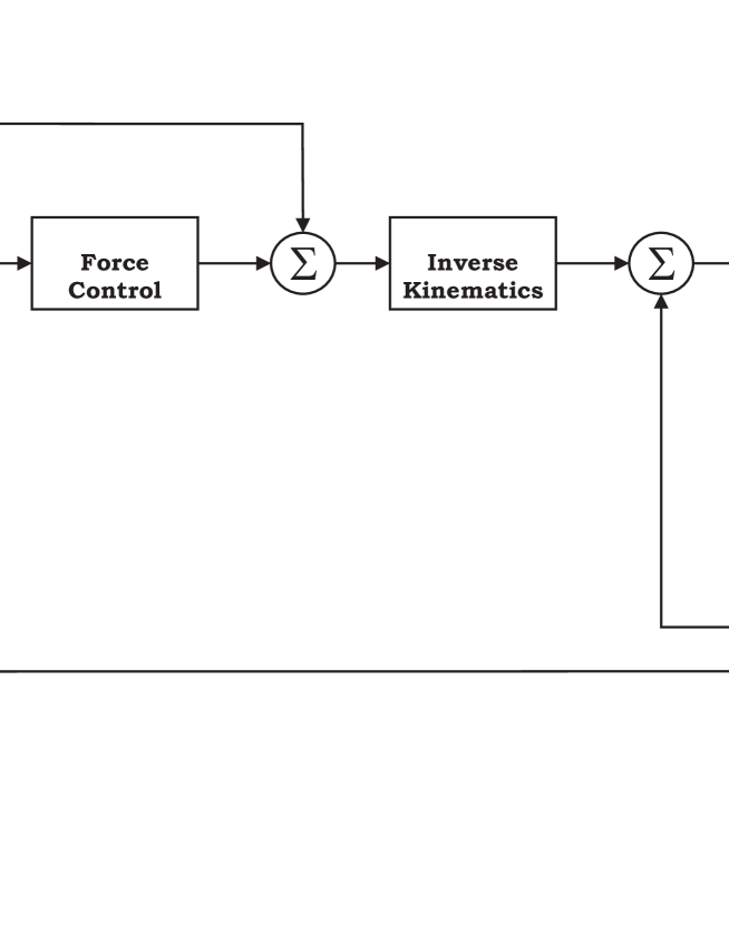
Figure 2: Implicit Force Controller for the flexible-link manipulator.

4 Tracking Control Loop

We propose a theorem that ensures the global asymptotic stability of the PD (Proportional-Derivative) tracking controller, with both gravity and vibration frequencies compensation on manipulator. The theorem (1), calculate the parameters of tuning of the tracking controller based on the dynamics of the manipulator. This parameters only depend of the structure of the beam and the spacial configuration of the manipulator.

Theorem 1.

Consider the nonlinear open-loop system $\dot{x}=f(x)+\varrho(x)u$, representing the rotation joint of the flexible-link manipulator, with $x-y$ workspace, under gravity influence. In order to define a closed-loop tracking controller using the control law:

$$u=K_{p}\tilde{\wp}+K_{v}\dot{\tilde{\wp}}+M(\wp)[\ddot{\wp}_{d}+\Delta\dot{\tilde{\wp}}]+C(\wp,\dot{\wp})[\dot{\wp}_{d}+\Delta{\tilde{\wp}}]+g(\wp)+\eta(\wp)$$ (16)

assuming that $\wp_{d}$ and $\dot{\wp}_{d}$ as a set of vector functions, $\ddot{\wp}_{d}$ is a constant and the closed-loop equation system-controller is non autonomous in the space then it can be assured that existence an unique equilibrium point, located at the origin and with global asymptotic stability for $K_{p}$ and $K_{v}$ $>0$, where $\tilde{\wp}$ and $\dot{\tilde{\wp}}$ are position velocity error vectors. The $K_{p}$ and $K_{v}$, are the proportional and derivative matrices and must be symmetric and positive, furthermore $\Delta=K_{v}^{-1}K_{p}$ must be a nonsingular matrix.

Proof 1.

1 Let the desired reference position $\wp_{d}$ for the controller be a feasible trajectory, defined in the manipulator workspace and the feedback control law given by the expression (17):

$$u=K_{p}\tilde{\wp}+K_{v}\dot{\tilde{\wp}}+M(\wp)[\ddot{\wp}_{d}+\Delta\dot{\tilde{\wp}}]+C(\wp,\dot{\wp})[\dot{\wp}_{d}+\Delta{\tilde{\wp}}]+g(\wp)+\eta(\wp)$$ (17)

where $K_{p}$ and $K_{v}$ $\in$ $\mathbb{R}^{nxn}$ are symmetric and positive definite matrices and $\Delta=K_{v}^{-1}K_{p}$ is a nonsingular matrix. Rewriting the control law (17) in functions of the $[\tilde{\wp}^{T}\quad\dot{\tilde{\wp}}]$, obtained the equation controller (22)

$$\frac{d}{dt}\left[\begin{array}[]{c}\tilde{\wp}\\ \dot{\tilde{\wp}}\end{array}\right]=\left[\begin{array}[]{c}\dot{\tilde{\wp}}\\ \frac{\Big{[}-K_{p}\tilde{\wp}-K_{v}\dot{\tilde{\wp}}-C(\wp,\dot{\wp})[\dot{\tilde{\wp}}+\Delta\tilde{\wp}]\Big{]}}{M(\wp)}\end{array}\right]$$ (22)

where (22) is a non autonomous differential equation, with an equilibrium point in the origin $[\tilde{\wp}^{T}\quad\dot{\tilde{\wp}}]=0$ $\varepsilon$ $\mathbb{R}^{2n}$.
The equation (23) will be used as the Lyapunov candidate function, this function is defined from dynamics of the manipulator.

$${\bigvee}(t,\tilde{\wp},\dot{\tilde{\wp}})=[\dot{\tilde{\wp}}+\Delta{\tilde{\wp}}]^{T}M(\wp)[\dot{\tilde{\wp}}+\Delta{\tilde{\wp}}]+\tilde{\wp}^{T}K_{p}\tilde{\wp}$$ (23)

According to statement of Robotics Theory, the inertia matrix $M(\wp)$ is symmetric and positive definite, and by definition $K_{p}$ is also symmetric and positive definite [11], it can be assured that $\bigvee$ is also globally positive definite. Replacing $K_{p}=K_{v}\Delta$ in $[\dot{\tilde{\wp}}+\Delta{\tilde{\wp}}]^{T}M(\wp)$ [12], we obtain:

$$\dot{\bigvee}(t,\tilde{\wp},\dot{\tilde{\wp}})=-\dot{\tilde{\wp}}^{T}K_{v}\dot{\tilde{\wp}}-\tilde{\wp}^{T}\Delta^{T}K_{v}\Delta\tilde{\wp}$$ (24)

Given that by definition $K_{v}$ is symmetric and positive definite and $\Delta$ is a nonsingular matrix, their product is positive definite, proving that $\dot{\bigvee}<0$ is a globally negative definite matrix. We can conclude that the system has global asymptotic stability in the theorem (1), for any symmetric positive definite matrix $K_{p}$ and $K_{v}$.

5 Force Controller

5.1 Force-Torque

In order to write (1), we can suppose that the manipulator end-effector is in contact with environment. In other hand, applying the virtual work principle [13], we can consider that the forces vector applied by the manipulator on the environment can be associated with the Jacobian (25), obtaining a finite dimensional model when the manipulator is it contact with the environment.

$$\tau_{e}=J(\wp)^{T}f_{c}$$ (25)

where the $J(\wp)$, is the Jacobian Matrix, that associates the velocity vector in the joint $\dot{\wp}$ with the velocity in the end-effector. In other words, a transformation from angular space to cartesian space. The Jacobian used in our expressions have been calculated directly of the end-effector position in cartesian space $P(x,y)$, considering the transversal deformations of the beam and $f_{c}$, as the contact force.

$$J(\wp)=\frac{\partial{P(x,y)}}{\partial\wp}$$ (26)

Since $P(x,y)$ is written in terms of $(\theta_{i},q_{ij})$, the kinematics velocity equation for the end-effector will be:

$$\dot{P}(x,y)=J_{\theta_{1}}(q)\dot{\theta}_{1}+J_{q_{11}}(q)\dot{q}_{11}+\ldots+J_{q_{1\nu}}(q)\dot{q}_{1\nu}$$ (27)

The mathematical model for the flexible manipulator has been developed for two vibration modes $(\nu=2)$, with the resulting Jacobian Matrix is:

$$\dot{P}(x,y)=J_{\theta_{1}}(q)\dot{\theta}_{1}+J_{q_{11}}(q)\dot{q}_{11}+J_{q_{1\nu}}(q)\dot{q}_{12}$$ (28)

$$\mathbf{J(\wp)}=\left[\begin{array}[]{lll}-l_{1}s1-w_{1}c1&-\phi_{11}(l_{1})s1&-\phi_{12}(l_{1})s1\\ -l_{1}c1-w_{1}s1&\phi_{11}(l_{1})c1&\phi_{12}(l_{1})c1\\ 0&0&0\\ 0&0&0\\ 0&0&0\\ 1&1&1\\ \end{array}\right]$$ (35)

5.2 Environment Model

The end-effector/contact-surface interaction is very difficult to model. In this case the environment has been modelled as a compliant environment without friction.

$$f_{c}=K_{e}\Big{[}P(x,y)-P_{0}(x,y)\Big{]}$$ (36)

The contact force $f_{c}$ have been representing as a position difference between end-effector $P(x,y)$ and contact point $P_{0}(x,y)$ more a $K_{e}$, that represent the environment stiffness coefficient. Since we consider a compliant environment, can be represent as a constant symmetric positive definite matrix.

5.3 Control Law

The implicit force control scheme was constructed as the outer loop that associates the contact force (36) with a position-velocity vector so that the difference between the desired force $(f_{d})$ and the contact force $(f_{c})$ can be translated to a position and velocity difference $\Delta P(x,y)$ and $\Delta\dot{P}(x,y)$ respectively, adding the last one to the reference signals of the tracking controller inner loop. In [14] an implicit force regulation scheme is proposed, with an outer force control PI, where the control law is given by (39), being the controller proportional contribution.

$$\dot{P}_{d}(x,y)=-K_{e}^{-1}k_{f}\int_{0}^{t}f(\tau)d\tau$$ (37)

$$\dot{P}_{d}(x,y)=-k\Delta f(t)=k[f_{c}(t)-f_{d}]$$ (38)

Where $k=K_{e}^{-1}k_{f}$, and integrating in time the position reference for the force control law:

$$P_{d}(x,y)=-K_{e}^{-1}k_{f}\int_{0}^{t}\Delta f(\tau)d\tau$$ (39)

Figure 3: Force/position-velocity relationship scheme control

5.4 Stability

In order to ensure the controller stability, we have defined our force controller based on (37) and (38), defining the velocity and position of the outer loop . Considering the desired force $f_{d}$ as a constant, the controller (37) ensure an asymptotically exact regulation, while the inner loop provides an asymptotically exact tracking. The inner velocity loops with bounded errors can be seen as:

$$\quad\lim_{t\rightarrow\infty}sup\|\Delta f(t)\|\leq\frac{1}{k_{f}}S$$ (40)

If $\lim_{t\rightarrow\infty}sup\|\Delta\dot{x}(t)\|\leq S$ and $S$ $\epsilon$ $\mathbb{R}^{n}$, then $0\leq S\leq\infty$ and $k_{f}>0$

$$\lim_{t\rightarrow\infty}sup\|\Delta\dot{x}(t)\|\leq S$$ (41)

6 Results and analysis

The proposed control scheme was tested using MatLab and Simulink. The simulations have been constructed so the manipulators end-effector was located in $P(x,y)=(0,0)m$ as the initial position. The environment was located in $P_{e}(x,y)=(0.7071,0.7071)m$, therefore the manipulator will be, at first, under the tracking controller action, until the end-effector makes contact with the environment. Once the contact is made, the force controller is activated. The simulations results are show it in the Fig.  4 and Fig.  5 for the one-link flexible manipulator. The parameters physical of the beam were: $1m.$ long aluminum beam with cross section diameter $10^{-3}m$, inertia $I_{m}=1.3254^{-06}Kgm^{2}$, elasticity coefficient $EI=34.3612Nm^{2}$, modes-shapes $\nu=2$. The parameters of the tracking controller are $K_{p}=diag[160\quad 100\quad 100]$, $K_{v}=diag[30\quad 1\quad 0.5]$. For the model of the environment $K_{e}=86.9N/m$ as stiffness coefficient of the environment. The force desired is $f_{d}=5N$. These results show that the end-effector reaches the final position desired applying to the environment the desired force. We also can observe that transversal deformations in stationary state converge to $error=0$.

(a)	(b)
(c)	(d)
(e)	(f)

Figure 4: Results of the Implicit Force Controller: $Environment=86.9N/m$, $fd=5N$.(a) Cartesian position end-effector in the axis $x$. (b) Cartesian position end-effector in the axis $y$ (c) Joint Position $\theta(t)$. (d) Transversal deformation $w(\hat{x},t)$. (e) First frequency of deformation E-B beam. (f) Second frequency of deformation E-B beam.

(a)

(b)

(c)

Figure 5: Results of the Implicit Force Controller: $Environment=86.9N/m$, $fd=5N$. (a) Total Force applied to environment. (b) Force component $F_{x}$ applied to the environment. (c) Force component $F_{y}$ applied to the environment.

Furthermore, in the Fig. 6, we are presenting as additional results the relation position-force, with three environments ($K_{e1}=20N/m$, $K_{e2}=86.4N/m$, $K_{e3}=200N/m$), this results proof as the environment is deform it, when the manipulator apply a force (verify the environment mathematical model), visualizing this deformation and parallel at this the convergence the both control loops ($error_{position}$ and $error_{force}$ $\rightarrow$ 0, in a finite time).

Figure 6: Relation Force-Position for enviroments with compliance variable.

7 Conclusion

This paper proposes a general method for implement a Implicit Force Controller based on dynamics of the manipulator. With the control scheme proposed is possible that the manipulator realize two works, considering indirectly the effect of the impact. The stability analysis was based on Lyapunov Theory, ensure the global asymptotic stability of the control scheme by obtaining a unique equilibrium point for controller constants $K_{p}$ and $K_{v}$, considering the compensation of the gravitational force and vibrational frequencies of the beam. Furthermore this method, can be used to prove of the resistance of materials, because is possible know the limits of the system (beam) associated with the vibrations amplitudes, before the deform completely when have been applied a reference force hight or when the environment is less compliant. The results were satisfactory and validate the proposed controller.

References

- [1] M. Raibert, J. Craig, Hybrid position-force control of manipulators., transactions of ASME, Journal of Dynamic Systems, Measurement and Control (102) (1981) 126–133.
- [2] T. Yoshikawa, Dynamics hybrid position/force control of robot manipulators-description of hand constraints and calculation of joints driving forces, In proceedings IEEE, Conference Robotics Automation (1986) 1393–1398.
- [3] T. Yoshikawa, Dynamics hybrid position/force control of manipulators description of hand constraints and calculation of joint driving force, IEEE Journal of Robotics and Automation Ra-3 (5) (1987) 386–392.
- [4] N. Hogan, Impedance control: an approach to manipulation: Theory, implementation, application, Journal of dynamic Systems, Measurement and Control,ASME 107.
- [5] D. Whitney, Historical perspective ans state of the art in robot force control, The Internartional Journal of Robotics Research 6 (1) (1987) 3–14.
- [6] C. Murrugarra, J. Grieco, G. Fernandez, M. Armada, Modelling of a 3d flexible manipulator: A generalized equation for n vibration frequencies, Measurement and Control in Robotics 1 (1) (2003) 199–204.
- [7] C. Murrugarra, J. Grieco, G. Fernandez, O. De Castro, A generalized mathematical model for flexible link manipulators with n vibration frequencies and friction in the joint, ISRA 2006, International Symposium on Robotics and Automation 1 (1) (2006) 23–28.
-
[8]
M. Spong, S. Hutchinson, M. Vidyasagar,
Robot Modeling and
Control, Wiley, 2005.
URL https://books.google.com.co/books?id=wGapQAAACAAJ - [9] W. Thomson, Theory of Vibration with Applications, 5th Edition, Prentice Hall, USA, 1993.
- [10] S. Moorehead, Position and force control of flexible manipulators, Master’s thesis, University of Waterloo, Waterloo,Ontario, Canada (1996).
- [11] C. Murrugarra, J. Grieco, G. Fernandez, O. De Castro, Design of a pd position control based on the lyapunov theory for a robot manipulator flexible-link, Proceedings IEEE International Conference on Robotics and Biomimetics ROBIO 2006. 1 (1).
- [12] R. Kelly, V. Santibáñez, Control de Movimiento de Robots Manipuladores., Pearson Prentice Hall, Spain, 2003.
- [13] L. Meirovitch, Dynamics and Control of Structures, Wiley Interscience Publication, USA, 1990.
- [14] J. De-Shutter, H. Van-Brussel, Compliant robot motion ii. a control approach based on external control loops, The Internartional Journal of Robotics Research 7 (4) (1988) 18–33.