Spectral shapes of forbidden argon $\beta$ decays as background component for rare-event searches

Abstract

The spectral shape of the electrons from the two first-forbidden unique $\beta^{-}$ decays of ³⁹Ar and ⁴²Ar were calculated for the first time to the next-to-leading order. Especially the spectral shape of the ³⁹Ar decay can be used to characterise this background component for dark matter searches based on argon. Alternatively, due to the low thresholds of these experiments, the spectral shape can be investigated over a wide energy range with high statistics and thus allow a sensitive comparison with the theoretical predictions. This might lead to interesting results for the ratio of the weak vector and axial-vector constants in nuclei.

1 Introduction

Liquid Argon (LAr) as a detection material is widely used in nuclear and particle physics with new applications coming in. The range covers calorimetry in high-energy-physics experiments at LHC all the way to large-scale low-background experiments for rare-event searches, especially dark matter. In addition, a 40 kiloton scale LArTPC detector is envisaged for the DUNE [1] long-baseline neutrino program. The GERDA experiment [2], searching for neutrino-less double beta decay using Ge-semiconductor detectors, is cooling its detectors with LAr.

The focus of this paper is on the low-background section of the potential experiments, especially dark matter experiments, of which two ongoing LAr experiments are DEAP-3600 [3] and DarkSide-50 [4]. The question arises whether there are additional background contributions from the Ar itself. Indeed, Ar has three long-living nuclides, ³⁷Ar, ³⁹Ar and ⁴²Ar, which deserve some attention. First, there is the well-known ³⁷Ar with a half-life of 35 days, which was the signal of the Homestake experiment for the radiochemical detection of solar neutrinos using a ³⁷Cl detector [5]. This isotope decays via electron capture (EC) without emission of gamma rays, but it will produce X-ray lines below 10 keV. The isotope ³⁷Ar might be produced by thermal neutron captures on ³⁶Ar, but this nuclide has only a small abundance of 0.337 %. More severe contaminants are the long-living nuclides ³⁹Ar and ⁴²Ar, which we will discuss now in a bit more in detail.

The decay of both isotopes into the ground state of the corresponding daughter nucleus is characterised as first-forbidden unique $\beta^{-}$-decay: ($\frac{7}{2}^{+}\rightarrow\frac{3}{2}^{-}$) for ³⁹Ar and ($0^{+}\rightarrow{2}^{-}$) for ⁴²Ar. The $\beta$-decay endpoints are given by 565 $\pm$ 5 keV (³⁹Ar) and 599 $\pm$ 6 keV (⁴²Ar), respectively [7]. The measured half-lives for ³⁹Ar are 265 $\pm 30$ years [8] and 269$\pm$ 3 years [9]. Its content is on the level of 10 mBq/m³ [11] and the specific activity was measured by the WARP experiment to be $1.01\pm 0.02\pm 0.08$ Bq per kg of natural Ar [10]. The current accepted half-life for ⁴²Ar is 32.9 $\pm 1.1$ years [9]. In none of the publications a $\beta$-spectrum of the corresponding Ar beta decay is shown.

In this paper we study the $\beta$-decay spectral shapes of the two isotopes ³⁹Ar and ⁴²Ar. We calculate the shapes using up to date nuclear models. In this way we plan to predict the expected $\beta$-spectrum shape for the Ar-based dark-matter experiments and, on the other hand, encourage the experimentalists to provide a spectrum which can be compared with theory.

2 Calculation of the spectral shape of ³⁹Ar and ⁴²Ar

In order to simplify the nuclear $\beta^{-}$-decay theory enough to allow us to do practical calculations we use the so-called impulse approximation in which at the exact moment of decay the decaying nucleon only feels the weak interaction [12]. The strong interaction with the remaining $A-1$ nucleons is ignored, and thus the pion exchange and other many-body effects are neglected. In the impulse approximation a neutron decays into a proton via emission of a massive $W^{-}$ vector boson which in turn decays into an electron and an anti-neutrino. Due to the large mass of the $W^{-}$ boson in comparison to the energy scale of the nuclear beta decay, the $W^{-}$ boson couplings to the baryon and lepton vertices, with weak-interaction coupling strength $g_{\rm W}$, can be approximated as a single effective interaction vertex with effective coupling strength $G_{\rm F}$, the Fermi constant. When the decay process is described with the effective point-like interaction vertex, the probability of the electron being emitted with kinetic energy between $W_{e}$ and $W_{e}+dW_{e}$ is

$$P(W_{e})dW_{e}= \frac{G_{\rm F}}{(\hbar c)^{6}}\frac{1}{2\pi^{3}\hbar}C(W_{e})$$

$$\times p_{e}cW_{e}(W_{0}-W_{e})^{2}F_{0}(Z,W_{e})dW_{e}\,,$$ (1)

where $p_{e}$ is the momentum of the electron, $Z$ is the proton number, $F_{0}(Z,W_{e})$ is the Fermi function, and $W_{0}$ is the end-point energy of the $\beta$ spectrum. The nuclear-structure information is in the shape factor $C(w_{e})$. Integrating Eq. (1) over the possible electron energies gives the total transition probability, and thus the half-life of the $\beta^{-}$ decay.

The half-life of a $\beta$ decay can be written as

$$t_{1/2}=\frac{\rm ln\ (2)}{\int_{m_{e}c^{2}}^{W_{0}}P(W_{e})dW_{e}}:=\frac{\kappa}{\tilde{C}}\,,$$ (2)

where $\tilde{C}$ is the integrated shape factor and the constant $\kappa$ has the value [13]

$$\kappa=\frac{2\pi^{3}\hbar^{7}\mathrm{ln\ 2}}{m_{e}^{5}c^{4}(G_{\rm F}\cos\theta_{\rm C})^{2}}=6147\ \mathrm{s}\,,$$ (3)

$\theta_{\rm C}$ being the Cabibbo angle. In order to simplify the formalism it is usual to introduce unitless kinematic quantities $w_{e}=W_{e}/m_{e}c^{2}$, $w_{0}=W_{0}/m_{e}c^{2}$, and $p=p_{e}c/(m_{e}c^{2})=\sqrt{w_{e}^{2}-1}$. With the unitless quantities the integrated shape factor can be expressed as

$$\tilde{C}=\int^{w_{0}}_{1}C(w_{e})pw_{e}(w_{0}-w_{e})^{2}F_{0}(Z,w_{e})dw_{e}\,.$$ (4)

The characteristics of the electron spectrum are encoded in the shape factor $C(w_{e})$, which can be expressed as [14]

$$C(w_{e})= \sum_{k_{e},k_{\nu},K}\lambda_{k_{e}}\Big{[}M_{K}(k_{e},k_{\nu})^{2}+m_{K}(k_{e},k_{\nu})^{2}$$

$$-\frac{2\gamma_{k_{e}}}{k_{e}w_{e}}M_{K}(k_{e},k_{\nu})m_{K}(k_{e},k_{\nu})\Big{]}\,,$$ (5)

where $k_{e}$ and $k_{\nu}$ (both running through 1,2,3,…) emerge from the partial-wave expansion of the electron and neutrino wave functions, $\gamma_{k_{e}}=\sqrt{k_{e}^{2}-(\alpha Z)^{2}}$, and $\lambda_{k_{e}}=F_{k_{e}-1}(Z,w_{e})/F_{0}(Z,w_{e})$ is the Coulomb function where $F_{k_{e}-1}(Z,w_{e})$ is the generalized Fermi function. The largest contributions to the sum of Eq. (5) come from the terms with minimal angular-momentum transfer, so in the case of the unique forbidden decays studied in this work, we only consider the sum that satisfies the condition $k_{e}+k_{\nu}=K+2$. The quantities $M_{K}(k_{e},k_{\nu})$ and $m_{K}(k_{e},k_{\nu})$ have lengthy expressions involving kinematic and nuclear form factors. The explicit expressions can be found from [14] (the expressions were also given in the recent article [15]). The form factors appearing in these expressions can be expanded as power series of $qR/\hbar$ as

$$\mathcal{F}_{\rm KLS}(q^{2})=\sum_{N}\frac{(-1)^{N}(2L+1)!!}{(2N)!!(2L+2L+1)!!}(qR/\hbar)^{2N}\mathcal{F}^{(N)}_{\rm KLS}\,,$$ (6)

where $q=|p_{e}+p_{\nu}|$ and $R$ is the nuclear radius. In practical calculations the quantities $M_{K}(k_{e},k_{\nu})$ and $m_{K}(k_{e},k_{\nu})$ are expanded as a power series of the quantities $\eta_{1,2,3,4,5}=\alpha Z$, $p_{e}R/\hbar$, $qR/\hbar$, $m_{e}cR/\hbar$, and $W_{e}R/\hbar c$. $M_{K}(k_{e},k_{\nu})$ and $m_{K}(k_{e},k_{\nu})$ consist of terms proportional to $\prod_{i}\eta_{i}^{\alpha_{i}}\mathcal{F}_{\rm KLS}$, where $\alpha_{i}=0,1,2,3,4,5$. In the case of the unique decays the often used leading-order approximation takes into account only the $(p_{e}R/\hbar)^{k_{e}-1}(qR/\hbar)^{k_{\nu-1}}$ term, while the here adopted next-to-leading-order treatment [15] takes into account also the $(p_{e}R/\hbar)^{k_{e}-1}(qR/\hbar)^{k_{\nu-1}}\eta_{j}$ terms. The leading-order and next-to-leading-order expressions of the $\beta$-decay shape factor are discussed in detail in Ref. [15] for a more general framework including also the (more involved) non-unique forbidden decays.

In the impulse approximation the nuclear form factors can be replaced by nuclear matrix elements (NMEs) [14]. In the leading-order approximation there is only one NME contributing to the shape factor for the unique decays. Therefore, the spectrum-shape and the half-life are proportional to $g_{\rm A}^{-2}$, where $g_{\rm A}$ is the weak axial-vector coupling constant. When the next-to-leading-order terms are taken into account, the number of contributing NMEs increases to five, with each NME carrying a prefactor $g_{\rm A}$ or $g_{\rm V}$ (weak vector coupling constant). As a result, the shape factor can be expressed as a decomposition

$$C(w_{e})=g_{\rm V}^{2}C_{\rm V}(w_{e})+g_{\rm A}^{2}C_{\rm A}(w_{e})+g_{\rm V}g_{\rm A}C_{\rm VA}(w_{e})\,.$$ (7)

In the here adopted next-to-leading-order theory the dependence on the weak coupling constants of the spectrum shape for the studied decays of Argon isotopes is, at least theoretically, non-trivial.

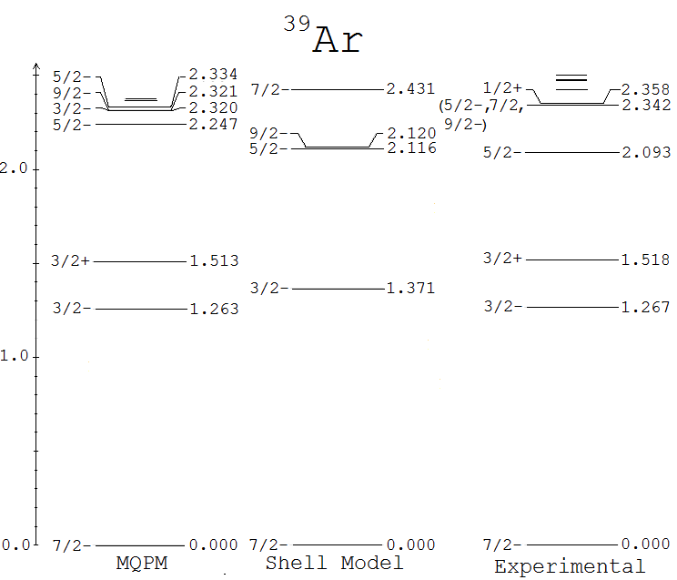
Figure 1: The excitation spectrum of ${}^{39}\rm Ar$ calculated using the MQPM and the shell model. The experimental excitation spectrum is from [16].

The choice of a nuclear model enters the picture when calculating the one-body transition densities (OBTDs) needed for the evaluation of the NMEs related to the transition. In this work the wave functions of the initial and final states were calculated using the microscopic quasiparticle-phonon model (MQPM) [17, 18] and the nuclear shell model. The MQPM is a fully microscopic model which can be used to describe spherical odd-$A$ nuclei, in the case of this work ${}^{39}\rm Ar$ and ${}^{39}\rm K$. In the MQPM the states of the odd-$A$ nucleus are built from BCS quasiparticles and their couplings to QRPA phonons. The quasiparticles and phonons emerge from the calculations done on the neighboring even-even reference nucleus (here ${}^{38}\rm Ar$). The MQPM has previously been used in the calculations of forbidden beta-decay spectrum shapes in Refs. [15, 19, 20].

The practical application of the MQPM model follows the same basic steps as in the earlier studies (see Refs. [15, 18, 19, 20, 21, 22]) including the use of the Bonn one-boson-exchange potential with G-matrix techniques [18]. The single-particle energies, used to solve the BCS equations, were calculated using the Coulomb-corrected Woods-Saxon potential with the Bohr-Mottelson parametrization [23]. The valence space spanned the orbitals $0s0p1s0d0f1p0g_{9/2}$. The BCS one-quasiparticle spectra were tuned by adjusting manually some of the key single-particle energies to get a closer match between the low-lying one-quasiparticle states and the corresponding experimental ones. The empirical pairing gaps, computed using the data from [6], were adjusted to fit the computed ones by tuning the pairing strength parameters $g_{\rm pair}^{\rm p}$ and $g_{\rm pair}^{\rm n}$ for protons and neutrons separately. In the MQPM calculations an extended cutoff energy of 6.0 MeV was used for the QRPA phonons instead of the 3.0-MeV cutoff energy used in Refs. [19, 20].

The shell-model OBTDs were calculated using the shell-model code NuShellX@MSU [24] with the effective interaction sdpfnow [25], tuned for the $1s0d0f1p$ valence space. Since performing a shell-model calculation in the entire half-filled $1s0d0f1p$ valence space would be impossible due to the extremely large dimensions of the shell-model Hamiltonian matrix, some controlled truncations were made. We limited the protons to the $sd$-shell, leaving the $fp$-shell empty, and forced a complete filling of the $sd$-shell for neutrons, leaving the entire $fp$-shell as the neutron valence space. These truncations are reasonable since we are only interested in the ground-state wave functions, to which configurations opening the neutron $sd$-shell and proton configurations with protons in the $fp$-shell have very small contributions due to the considerable energy gap between the two shells. The adopted shell-model Hamiltonian predicts correctly the spin-parities of the low-lying states in the studied nuclei. As an example, the energy spectra of ${}^{39}\rm Ar$, predicted by the MQPM and shell model, are compared with the experimental spectrum [16] in Fig. 1. In the shell-model spectrum the positive-parity states are missing, since the odd neutron is restricted to the $fp$-shell.

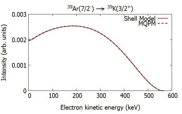
Figure 2: Electron spectrum of the ground-state-to-ground-state decay of ${}^{39}\rm Ar$ calculated using the MQPM and the shell model with the effective interaction sdpfnow [25]. The experimental spectrum is from NNDC [16].

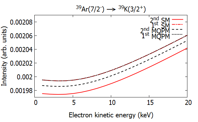
Figure 3: Zoom-in of the low-energy end of the electron spectrum of ${}^{39}\rm Ar$ calculated using the shell model (SM) and the microscopic quasiparticle-phonon model (MQPM) with leading-order (1st) and next-to-leading-order (2nd) terms of the shape factor $C(w_{e})$ included. The values $g_{\rm A}=g_{\rm V}=1.00$ were adopted. Note the range on the $y$-axis.

Figure 4: Zoom-in of the low-energy end of the electron spectrum of ${}^{39}\rm Ar$ calculated using the shell model. The color/dash coding refers to the ratio $g_{\rm A}/g_{\rm V}$. Note the range on the $y$-axis.

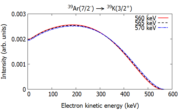
Figure 5: Electron spectrum of ${}^{39}\rm Ar$ calculated using the shell model and the experimental Q-value $656\pm 5$ keV [6]. The next-to-leading-order terms are included and the values $g_{\rm A}=g_{\rm V}=1.00$ were adopted.

Figure 6: Electron spectrum of the ground-state-to-ground-state decay of ${}^{42}\rm Ar$ calculated using the shell model with the effective interaction sdpfnow [25]. The experimental spectrum is from NNDC [16].

The electron spectrum of the ${}^{39}\rm Ar$ decay is presented in Fig. 2. Here the next-to-leading-order terms are taken into account and the values $g_{\rm V}=g_{\rm A}=1$ were adopted for the weak coupling constants. The spectra were calculated also using the $g_{\rm A}/g_{\rm V}$ ratios $0.8-1.2$ but the spectra coincided perfectly, meaning that the possible dependence of the spectrum shape on the weak coupling constants is very weak. The spectra calculated using the shell model and the MQPM agree also extremely well, suggesting that the uncertainty related to the wave functions of the initial and final states is tiny. The difference between the two spectra is largest at the low-energy end, while at the high-energy end the spectra coincide perfectly. In Fig. 3 a zoom-in of the low-energy part of the spectrum is presented, with the next-to-leading-order terms of the shape factor either included or neglected. The difference in the intensities predicted by the two models, with the next-to-leading-order terms included, is at most $0.5\%$ of the intensity.

When the next-to-leading-order-terms are taken into account, the dependence of the shape-factor on the ratio $g_{\rm A}/g_{\rm V}$ becomes non-trivial for the unique forbidden decays. The difference between the ${}^{39}\rm Ar$ spectra calculated using different values of $g_{\rm A}/g_{\rm V}$ is largest at the low-energy end. The magnified low-energy shell-model electron spectrum is presented in Fig. 4. With larger quenching of $g_{\rm A}$, the intensity of the low-energy electrons increase slightly, but the difference is negligible within the accuracy of practical measurements.

The final source of uncertainty of the spectrum shape is the uncertainty related to the Q-value. The current experimental Q-value of the ${}^{39}\rm Ar$ decay is $565\pm 5$ keV. The shell-model spectra with Q-values 560, 565, and 570 keV are plotted in Fig. 5. Here a small difference between the spectra can be seen without further magnification. The uncertainty related to the Q-value seems to be by far the largest contributor to the uncertainty in the theoretical spectrum-shape. The change in Q-value stretches the spectrum, but the overall shape does not change.

For the ${}^{42}\rm Ar$ ground-state-to-ground-state decay the MQPM cannot be applied. The uncertainties related to the wave functions were negligible in the case of ${}^{39}\rm Ar$, as well as in the several other first-forbidden unique decays studied in Ref. [20], so the application of only one nuclear model should be sufficient. The electron spectrum is presented in Fig. 6. Again, there is no significant dependence on the values of $g_{\rm A}$ and $g_{\rm V}$. For the decay of the ${}^{42}\rm Ar$ isotope the experimental uncertainty of the Q-value is at 6 keV, similar to that of the ${}^{39}\rm Ar$ isotope, and thus the uncertainty of the spectrum-shape is also of a similar magnitude.

3 Summary and conclusions

In this paper the $\beta$ spectra of first-forbidden unique decays of ³⁹Ar and ⁴²Ar were calculated for the first time using a next-to-leading-order weak theory. The involved nuclear wave functions were computed by using the nuclear shell model and the microscopic quasiparticle-phonon model. The major uncertainty in studies of the speactral shapes is related to the uncertainty of the Q-value. Among the different calculations only very tiny differences could be observed at low energy of the $\beta$ spectrum, which can be studied in detail with running or future LAr dark-matter detectors, as they are sensitive in this energy range. This high sensitivity might allow to explore the $g_{\rm A}/g_{\rm V}$ ratio of the weak coupling constants. The higher-energy part of the $\beta$ spectrum of ³⁹Ar can already be seen in the released spectra of the GERDA experiment, but the lower-energy part might be disturbed due to dead-layer effects of the Ge detectors. To summarise, the calculated $\beta$ spectra can help to characterise the background contribution of the two studied isotopes for dark-matter searches based on LAr dark-matter detectors. On the other hand, these experiments can investigate the presently predicted spectral shape in detail as the expected decay rate, especially for ³⁹Ar, is reasonably high in these detectors.

4 Acknowledgement

This work was partly supported by the Academy of Finland under the Finnish Center of Excellence Program 2012-2017 (Nuclear and Accelerator Based Program at JYFL).

References

References

- [1] R. Acciarri et al., arXiv.1512.06148
- [2] K. H. Ackermann et al., Euro. Phys. J. C 2013 73, 2330
- [3] P. A. Amaudruz et al., 2016 , 340
- [4] P. Agnes et al., Phys. Lett. B 2015 743, 456
- [5] B. T. Cleveland et al., ApJ 1998 496, 505
- [6] M. Wang et al., Chin. Phys. C 2012 36, 1603
- [7] M. Wang et al., Chin. Phys. C 2017 41, 030003
- [8] H. Zeldes et al., Phys. Rev. 1952 86, 811
- [9] R. W. Stoenner, O. A. Schaeffer, S. Katcoff, Science 1965 148, 1325
- [10] P. Benetti et al., Nucl. Instrum. Methods A 2007 574, 83
- [11] H. H. Loosli, Earth Plan. Sci. Lett. 1983 63, 51
- [12] J. Suhonen, From Nucleons to Nucleus: Concepts in Microscopic Nuclear Theory, Springer, Berlin (2007)
- [13] J. C. Hardy et al., Nucl. Phys. A 1990 509, 429
- [14] H. Behrens and W. Bühring, Electron Radial Wave Functions and Nuclear Beta Decay, Clarendon, Oxdord (1982)
- [15] M. Haaranen et al., Phys. Rev. C 2017 95, 024327
- [16] National Nuclear Data Center, Brookhaven National Laboratory, www.nndc.bnl.gov
- [17] J. Toivanen et al., Journal of Physics G 1995 21, 1491
- [18] J. Toivanen et al., Phys. Rev. C 1998 57, 1237
- [19] M. Haaranen et al., Phys. Rev. C 2016 93, 034308
- [20] J. Kostensalo et al., Phys. Rev. C 2017 95, 044313
- [21] M. T. Mustonen et al., Phys. Rev. C 2006 73, 054301
- [22] M. Haaranen et al., Euro. Phys. J. A 2013 19, 93
- [23] A. Bohr and B. R. Mottelson, Nuclear Structure Vol I, Benjamin, New York (1969)
- [24] B. A. Brown et al., Nuclear Data Sheets 2014 120, 115
- [25] S. Nummela et al., Phys. Rev. C 2001 63, 044316