Magneto-Vortical evolution of QGP in heavy ion collisions

Abstract

The interplay of magnetic field and thermal vorticity in a relativistic ideal fluid might generate fluid vorticity during the fluid evolution provided the flow fields and the entropy density of the fluid is inhomogeneous Mahajan:2010 . Exploiting this fact and assuming large magnetic Reynolds number we study the evolution of generalised magnetic field ($\hat{B}$) which is defined as a combination of the usual magnetic field ($\vec{B}$) and relativistic thermal vorticity ($\omega^{\mu\nu}$), in a 2(space)+1(time) dimensional isentropic evolution of Quark Gluon Plasma (QGP) with longitudinal boost invariance. The temporal evolution of $\hat{B}$ is found to be different than $\vec{B}$ , and the $\hat{B}$ evolution also depends on the position of the fluid along the beam direction (taken along the z axis) with respect to the mid-plane $z=0$. Further it is observed that the transverse components ($\hat{B_{x}}$, $\hat{B_{y}}$) evolve differently around the mid-plane.

PACS numbers

25.75.-q, 12.38.Mh, 25.75.Ag

I Introduction

Understanding the space-time evolution of intense electromagnetic field produced in the initial stage of heavy ion collisions is an important subject, particularly the interplay of magnetic field and quantum anomalies, which includes the chiral magnetic effect Kharzeev:2007jp ; Fukushima:2008xe , chiral magnetic wave Burnier:2011bf , chiral vortical effect Kharzeev:2010gr etc. There are several other theoretical studies on the possible effects of large magnetic field in the initial stage of heavy ion collisions. For example, flow harmonics and fluid flow are shown to be altered in presence of non-zero magnetic field along the perpendicular direction to the participant plane Pang:2016yuh ; Inghirami:2016iru ; Das:2017qfi ; Greif:2017irh ; Roy:2015kma ; Pu:2016bxy . Transport coefficients of nuclear matter might also be changed under the influence of strong electro-magnetic fields McInnes:2017ohn ; Tawfik:2016ihn ; Hattori:2016cnt .

It is now widely accepted view that due to the relativistic speed of the charged protons inside the colliding nucleus a magnetic field as large as $\sim 10^{19}$ Gauss is produced in mid-central Au+Au collisions at $\sqrt{s_{\rm NN}}=$ 200 GeV Deng:2012pc ; Bzdak:2011yy ; Roy:2015coa . The magnitude of this initial electromagnetic field increases almost linearly as a function of $\sqrt{s_{\rm NN}}$ Deng:2012pc . However, the subsequent space-time evolution of the initial magnetic field inside the Quark Gluon Plasma (QGP - deconfined state of partons created in the heavy-ion collisions Gyulassy:2004zy ; Adams:2005dq ) is still uncertain. The main uncertainty comes from the poorly known value of the electrical conductivity $\sigma_{e}$ in the QGP Gupta:2003zh ; Qin:2013aaa ; Arnold:2000dr phase and in the subsequent hadronic phase Greif:2016skc ; Steinert:2013fza ; Ghosh:2016yvt .

The space-time evolution of QGP (which contains electrically charged quarks) in the presence of magnetic field is governed by the relativistic magneto-hydrodynamic (MHD) equations. Depending on the value of magnetic Reynolds number $R_{m}=\sigma_{e}vl\mu$, where $l$ is some characteristic length scale of the QGP; $v$ is the fluid velocity; $\mu$ is the magnetic permeability of the QGP, one can approximate the MHD evolution as ideal (when $R_{m}\gg 1$) or resistive ($R_{m}\ll 1$) Goedbloed:2008 . To get an order of magnitude estimate of $R_{m}$, let us consider that in heavy ion collisions at top RHIC energy the typical fluid velocity is $v\sim 0.5c$, the QGP possesses large electrical conductivity $\sigma_{e}\sim 6T/e^{2}$ Arnold:2000dr at temperature $T=300$ $MeV$, assuming $\mu=1$ and $l=10$ $fm$ we have $R_{m}\sim 560$. Hence as $R_{m}\gg 1$ one can treat the QGP evolution within the framework of ideal MHD. However, note that it is still an open question whether the QGP is in ideal MHD regime or in the resistive regime, for example Tuchin:2013apa uses resistive MHD limit.

We know that in the initial stage of heavy ion collisions (particularly in non-central collisions) the colliding nucleus carry large angular momentum Becattini:2007sr . A fraction of this large angular momentum might give rise to finite fluid vorticity Becattini:2015ska ; Pang:2016igs ; Li:2017dan . The existence of strong magnetic fields and large flow vorticity in the reaction zone may have interesting consequences. In fact, in classical physics, the Larmor’s theorem states that the motion of a charged particle in a magnetic field $\vec{B}$ is equivalent to the motion in a rotating frame with angular velocity $\omega=q\vec{B}/(2m)$ with an additional centrifugal force, where $m$ and $q$ are the mass and charge of the particle under consideration.

Magnetic field and fluid vorticity can be coupled together and they follow a generalized form of advection equation Mahajan:2003 ; Mahajan:2010 . The origin of this generalized form of coupled magneto-vortical evolution trace back to the fact that the equations governing fluid vorticity and magnetic field is of common form and we can take a linear combination of both of them Steinhauer:1997 . It is a well known fact that in the limit of vanishing electrical conductivity, plasma retains the initial magnetic flux passing through it, this phenomenon is known as frozen of magnetic flux. In this case the electric and magnetic fields are no longer independent entities and are related as $\vec{E}=-\vec{v}\times\vec{B}$. The relativistic formulation of the problem requires a proper choice of fluid vorticity. The fluid vorticity could take many different forms, one of them is the thermal vorticity $\omega^{\mu\nu}=\partial^{\nu}\left(fu^{\mu}\right)-\partial^{\mu}\left(fu^{\nu}\right)$ Luciano:2013 ; Lich:1967 , where $f(T)$ is in general a function of temperature, $u^{\mu}=(\gamma,\gamma\vec{v})$ is the fluid 4-velocity, and $\gamma=1/\sqrt{1-v^{2}}$ being the relativistic kinematic factor (see Appendix B for details). Note that $\omega^{\mu\nu}$ is actually different than its non-relativistic counterpart $\vec{\omega}=\vec{\nabla}\times\vec{v}$. From now on we shall refer the thermal vorticity as vorticity unless stated otherwise.

In this work we consider an ideal (zero viscosity and vanishing electrical resistivity) QGP expanding under external homogeneous time varying magnetic field. Since the electrical ressitivity of the fluid is very small we use ideal MHD approximation. The aim is to study the temporal evolution of the generalized magnetic field (initial magnetic field coupled to vorticity) within a relativistic framework. We note that the authors of Deng:2012pc have attempted to address similar problem for a 2+1 dimensional expansion of QGP under external magnetic field. However our work is different as it incorporates the both magnetic field and fluid vorticity effects. In addition we have also considered relativistic correction to the evolution equation.

It is worthwhile to point out that in order to investigate the space-time evolution of plasma and associated electromagnetic field one should solve the complete set of relativistic magnetohydrodynamics equations with a proper initial condition and appropriate Equation of State (EoS). Recently few group have started investigating the magneto-hydrodynamical evolution of QGP by numerically solving the corresponding energy momentum tensor Pang:2016yuh ; Inghirami:2016iru ; Das:2017qfi ; Greif:2017irh ; Roy:2015kma , but none of the existing numerical codes solve the magnetohydrodynamics equation self consistently and at the same time consider non-zero fluid vorticity.

The rest of the paper is organized as follows: in the next section we discuss the theoretical formulation and results. Section III contains summary of our findings. We have re-derive some useful formulae associated with this study and those are given in the Appendix A and B for completeness. Throughout the paper we use natural unit ($\hbar=c=k_{B}=1$ and the metric tensor $g^{\mu\nu}$= diagonal(1,-1,-1,-1). Four vectors are denoted by Greek indices, three vectors are denoted by arrow.

II Formulation and result

To set the stage one must begin with earliest non relativistic induction equation of MHD

$$\frac{\partial\widetilde{B}}{\partial t}-\vec{\nabla}\times\left(\vec{v}\times\widetilde{B}\right)=-\vec{\nabla}{n}^{-1}\times\vec{\nabla}p=\vec{\nabla}T\times\vec{\nabla}\left(\frac{s}{n}\right)$$ (1)

where the term $\widetilde{B}=\vec{\omega}+q\vec{B}$ is called the generalised magnetic field (or generalised vorticity) combines the fluid vorticity $\vec{\omega}=\vec{\nabla}\times\vec{v}$ and magnetic field $\vec{B}=\vec{\nabla}\times\vec{A}$ (where $\vec{A}$ is the usual vector potential) together in a single equation. Note that in the right hand side of Eq.(1) we have used the thermodynamic relation

$$d\left(\frac{h}{n}\right)=Td\left(\frac{s}{n}\right)+\frac{1}{n}dp$$ (2)

where $h$ is the enthalpy density, $s$ is the entropy density, $p$ is pressure and $T$ is the temperature of the fluid and $n$ is the number density Landau:1987 . If the plasma is barotropic , i.e., a fluid whose pressure is a function of the number density only, i.e., $p=p(n)$, or in other words the entropy density is a function of only temperature, i.e., $s=s(T)$ the right side of Eq.(1) is zero and the resulting ideal transport equation becomes

$$\frac{\partial\widetilde{B}}{\partial t}-\vec{\nabla}\times\left(\vec{v}\times\widetilde{B}\right)=0.$$ (3)

Both Kelvin’s circulation theorem in hydrodynamics and the frozen-in flux theorem of MHD, for example, are contained in Eq.(3) which states that for any loop $L(t)$ (or the enclosing surface $A(t)$) transported with the fluid, the circulation (or the flux) is conserved, i.e.,

$$\frac{d}{dt}\oint_{L(t)}\widetilde{P}\cdot d\vec{x}=\frac{d}{dt}\int_{A(t)}\widetilde{B}\cdot\hat{n}d^{2}x=0$$ (4)

where $\widetilde{P}=\vec{v}+q\vec{A}$. Note that the material derivative $d/dt=\partial/\partial t+\vec{v}\cdot\vec{\nabla}$.

But the same is not true for relativistic fluids. In principle we can combine the electromagnetic field tensor $F^{\mu\nu}$ and the flow field tensor ${\omega}^{\mu\nu}$, into an unified tensor $M^{\mu\nu}=qF^{\mu\nu}+\omega^{\mu\nu}$ (see Appendix B). Generalizing Kelvin’s theorem and the frozen-in flux theorem of MHD to relativistic fluids, forces us to switch to proper time loop $L(\tau)$ (where proper time $\tau=t/\gamma$) in Eq.(4). This transformation yields a Jacobian ${\gamma}^{-1}$ which makes the right hand side nonzero and we have (see Appendix B)

$$\frac{\partial\hat{B}}{\partial t}-\vec{\nabla}\times\left(\vec{v}\times\hat{B}\right)=\frac{\gamma T}{2q}\vec{\nabla}v^{2}\times\vec{\nabla}\left(\frac{s}{n}\right)-\frac{1}{q\gamma}\vec{\nabla}T\times\vec{\nabla}\left(\frac{s}{n}\right),$$ (5)

where the generalized magnetic field in the relativistic scenario is $\hat{B}=\vec{B}+\vec{\nabla}\times\left(f\gamma\vec{v}\right)$, $\vec{B}$ is the usual magnetic field, $f=\frac{h}{n}$ is the enthalpy density ($h$) per unit conserved charge ($n$), $q$ is the absolute magnitude of the electric charge of the fluid particles. Note that for $s(T)$ (which is generally true for hot and dense QGP) the second term on the right hand side yields zero but the first term might be non-zero. Thus for ideal relativistic barotropic fluid we have

$$\frac{\partial\hat{B}}{\partial t}-\vec{\nabla}\times\left(\vec{v}\times\hat{B}\right)=\frac{\gamma T}{2q}\vec{\nabla}v^{2}\times\vec{\nabla}\left(\frac{s}{n}\right)$$ (6)

The term in the right hand side of Eq.(6) has its origin in the space-time distortion caused by the demands of special relativity and is non existent in the non relativistic formulation. Following conclusion can be readily obtained from Eq.(6):

1. The relativistic induced term on the right of Eq.(6) is zero for homogeneous entropy density or for homogeneous flow fields.

2. It can also be zero if the term $\vec{\nabla}v^{2}$ is co-linear to $\vec{\nabla}s$.

Now we shall discuss an application of the above mentioned generalized relativistic case to high energy heavy ion collisions. We consider a 2+1 dimensional ideal MHD evolution of QGP. The velocity $v_{z}=\frac{z}{t}$ follow Bjorken one dimensional expansion along the longitudinal direction (along the beam axis). Following Ollitrault:2008zz we assume that the transverse expansion is slower compared to the longitudinal expansion. The fluid velocity in the transverse plane $\vec{v}_{\perp}=\hat{x}v_{x}+\hat{y}v_{y}$ is obtained from the following equation

$$\frac{\partial\vec{v}_{\perp}}{\partial t}=-c_{s}^{2}\nabla_{\perp}s$$ (7)

where, $c_{s}$ is the speed of sound, $s$ is entropy density of the fluid. For the present work we assume a Gaussian transverse entropy(or energy density) profile

$$s\left(x,y\right)=s_{0}exp\left(-\frac{(x-{\mu}_{x})^{2}}{2\sigma_{x}^{2}}-\frac{(y-{\mu}_{y})^{2}}{2\sigma_{y}^{2}}\right)$$ (8)

where $\sigma_{x}$ and $\sigma_{y}$ are the Gaussian width along $x$ and $y$ direction respectively, $s_{0}$ is the entropy density at $x={\mu}_{x},y={\mu}_{y}$, for simplicity we take ${\mu}_{x}={\mu}_{y}=0$. By using Eq.(8) into Eq.(7) a straightforward calculation gives

$$v_{x} = \frac{c_{s}^{2}x}{2\sigma_{x}^{2}}t$$ (9)

$$v_{y} = \frac{c_{s}^{2}y}{2\sigma_{y}^{2}}t$$ (10)

and according to the Bjorken assumption

$$v_{z}=\frac{z}{t}$$ (11)

The transverse and longitudinal displacement of the fluid can be readily obtained by integrating $\vec{v}$ with respect to time

$$x(t) = x_{0}\exp\left(\frac{c_{s}^{2}\left(t^{2}-t_{0}^{2}\right)}{2\sigma_{x}^{2}}\right)$$ (12)

$$y(t) = y_{0}\exp\left(\frac{c_{s}^{2}\left(t^{2}-t_{0}^{2}\right)}{2\sigma_{y}^{2}}\right)$$ (13)

$$z(t) = z_{0}\frac{t}{t_{0}}$$ (14)

where $x_{0},y_{0}$ and $z_{0}$ are the initial transverse and longitudinal positions of the fluid at time $t=t_{0}$.

As mentioned earlier we investigate the ideal MHD evolution of QGP with non-zero fluid vorticity. Note that according to the non-relativistic definition of vorticity $\vec{\omega}=\vec{\nabla}\times\vec{v}$, the fluid velocity $\vec{v}=\left(\frac{c_{s}^{2}x}{2\sigma_{x}^{2}}t,\frac{c_{s}^{2}y}{2\sigma_{y}^{2}}t,\frac{z}{t}\right)$ gives $\vec{\omega}=\left(0,0,0\right)$. However, considering the relativistic generalisation of vorticity $\omega^{\mu\nu}=\partial^{\nu}\left(fu^{\mu}\right)-\partial^{\mu}\left(fu^{\nu}\right)$ (see Appendix B) gives non-zero value for the given velocity profile. In addition to that the frozen-in flux theorem gets modified in the relativistic regime.

We take boost invariance along longitudinal direction and hence fluid properties depends only in the transverse direction near the mid rapidity. Note that the term on the right hand side of Eq.(6) appears due to the relativistic effects and non-zero vorticity, thus in the non-relativistic limit and vanishing vorticity one gets back the usual form of ideal MHD evolution of magnetic field.

$$\frac{\partial\vec{B}}{\partial t}=\vec{\nabla}\times\left(\vec{v}\times\vec{B}\right)$$ (15)

Using the above equation Deng:2012pc have found analytic solution of magnetic field evolution for 2+1 dimensional expansion of QGP in the ideal MHD limit which is discussed in Appendix A. Let us now consider Eq.(6) and investigate the consequence of non-zero vorticity, finite gradient of entropy density and fluid velocity in the relativistic generalization.

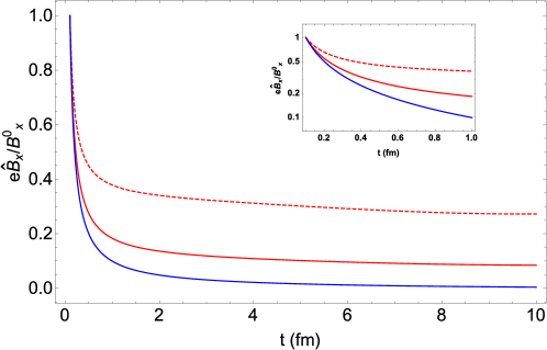
Figure 1: Temporal evolution of normalized $\hat{B}_{x}$ for z$>$0. Blue line corresonds to the usual magnetic field evolution, red solid line corresponds to $\hat{B}_{x}$ for $\gamma=3$, whereas red dashed line corresponds to $\hat{B}_{x}$ for $\gamma=10$. The inset figure shows the same result but with log scale.

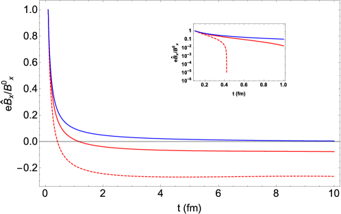
Figure 2: Same as Fig.1 but for z$<$0.

For simplicity let us consider that the net conserved charge $n$ is homogeneous and constant over the transverse plane. Note that $\vec{\nabla}v^{2}\times\vec{\nabla}s$= $s\left(\frac{2zy}{t^{2}\sigma_{y}^{2}},-\frac{2zx}{t^{2}\sigma_{x}^{2}},-2\left(\frac{xyg_{x}t^{2}}{\sigma_{y}^{2}}-\frac{xyg_{y}t^{2}}{\sigma_{x}^{2}}\right)\right)$, where $g_{x}=c_{s}^{4}/\sigma_{x}^{4}$ and $g_{y}=c_{s}^{4}/\sigma_{y}^{4}$. Thus from Eq.(6) we have the evolution equation of the component of $\hat{B}$

$$\frac{\partial\hat{B_{x}}}{\partial t}+\left(\frac{c_{s}^{2}t}{\sigma_{y}^{2}}+\frac{1}{t}\right)\hat{B_{x}} = \left(\frac{\gamma T}{2q}\right)\frac{2zy}{nt^{2}\sigma_{y}^{2}}s$$ (16)

$$\frac{\partial\hat{B_{y}}}{\partial t}+\left(\frac{c_{s}^{2}t}{\sigma_{x}^{2}}+\frac{1}{t}\right)\hat{B_{y}} = -\left(\frac{\gamma T}{2q}\right)\frac{2zx}{nt^{2}\sigma_{x}^{2}}s$$ (17)

Notice the different sign on the right hand side of Eq.(16) and (17), which will give rise to completely opposite evolution for $\hat{B}_{x}$ and $\hat{B}_{y}$. The solution also depends on the forward or backward rapidity ($z>0$,$z<0$). The solution of Eq.(16) and (17) can be found analytically. First note that setting right hand side of Eq.(16) and (17) to zero we have the homogeneous equations and the corresponding integrating factors are $M(t)=exp\left(\frac{c_{s}^{2}t^{2}}{2\sigma_{x}^{2}}\right)t$, and $N(t)=exp\left(\frac{c_{s}^{2}t^{2}}{2\sigma_{y}^{2}}\right)t$ respectively. Multiplying Eq.(16) and Eq.(17) by the corresponding integrating factors we have

$$\frac{\partial}{\partial t}\left(\hat{B_{x}}N(t)\right) = \left(\frac{\gamma T}{2q}\right)\frac{2szyN(t)}{nt^{2}\sigma_{y}^{2}}$$ (18)

$$\frac{\partial}{\partial t}\left(\hat{B_{y}}M(t)\right) = -\left(\frac{\gamma T}{2q}\right)\frac{2szxM(t)}{nt^{2}\sigma_{x}^{2}}$$ (19)

At this point we should use the explicit time dependence of $x(t),y(t),z(t),s(t)$, and $n(t)$ in order to solve Eq.(18) and (19). $x(t),y(t)$ and $z(t)$ are given in Eq.(12-14).

Here we shall use another assumption in order to evaluate $s(t)$ and $n(t)$. Initially the longitudinal expansion is much faster compared to the transverse expansion the entropy density evolves as

$$s(t)=\frac{s_{0}t_{0}}{t}$$ (20)

Similarly the number density $n(t)$ is given as

$$n(t)=\frac{n_{0}t_{0}}{t}.$$ (21)

In reality the time dependence may be somewhat different than given in Eq.(20), we envisage that will not change the qualitative nature of the solution we obtained here. Inserting the time dependence of the above mentioned quantities in Eq.(18) and (19) yields

$$\frac{\partial}{\partial t}\left(\hat{B}_{x}N(t)\right) = \left(\frac{\gamma T}{q}\right)C_{1}\exp\left(\frac{c_{s}^{2}(2t^{2}-t_{0}^{2})}{2\sigma_{y}^{2}}\right)$$ (22)

$$\frac{\partial}{\partial t}\left(\hat{B}_{y}M(t)\right) = -\left(\frac{\gamma T}{q}\right)C_{2}\exp\left(\frac{c_{s}^{2}(2t^{2}-t_{0}^{2})}{2\sigma_{x}^{2}}\right)$$ (23)

where $C_{1}=\frac{s_{0}z_{0}y_{0}}{n_{0}t_{0}\sigma_{y}^{2}}$, $C_{2}=\frac{s_{0}z_{0}x_{0}}{n_{0}t_{0}\sigma_{x}^{2}}$.

Integrating Eq.(22) and (23) with respect to time yields

$$\hat{B}_{x}=C_{1}\left(\frac{\gamma T}{q}\right)\frac{\sqrt{\pi}\sigma_{y}}{c_{s}t}\left[\operatorname{erfi}\left(\frac{c_{s}t}{\sigma_{y}}\right)-\operatorname{erfi}\left(\frac{c_{s}t_{0}}{\sigma_{y}}\right)\right]e^{-\frac{c_{s}^{2}(t^{2}-t_{0}^{2})}{2\sigma_{y}^{2}}}+\frac{B^{0}_{x}t_{0}}{t}e^{-\frac{c_{s}^{2}(t^{2}-t_{0}^{2})}{2\sigma_{y}^{2}}}$$ (24)

$$\hat{B}_{y}=-C_{2}\left(\frac{\gamma T}{q}\right)\frac{\sqrt{\pi}\sigma_{x}}{c_{s}t}\left[\operatorname{erfi}\left(\frac{c_{s}t}{\sigma_{x}}\right)-\operatorname{erfi}\left(\frac{c_{s}t_{0}}{\sigma_{x}}\right)\right]e^{-\frac{c_{s}^{2}(t^{2}-t_{0}^{2})}{2\sigma_{x}^{2}}}+\frac{B^{0}_{y}t_{0}}{t}e^{-\frac{c_{s}^{2}(t^{2}-t_{0}^{2})}{2\sigma_{x}^{2}}}$$ (25)

Eqs. (24) and (25) are the main result of this study. They describe the temporal evolution of $\hat{B}$ which includes both usual magnetic field (last term on the right hand side of both equations) and the relativistic correction (first term on the right hand side of both equations) arising due to non-zero vorticity and entropy gradient. Note that for a given $z$ the relativistic correction has opposite sign for $\hat{B}_{x}$ and $\hat{B}_{y}$. This is reflected in the numerical result shown in Fig.(1) and (2). Where we use the following values $s=100$ $MeV^{3}$, $n=0.4$ $MeV^{3}$, $T=200$ $MeV$, $\gamma=10$ (dashed lines) and $\gamma=3$ (solid lines), initial transverse coordinates $x_{0}=y_{0}=0.1$ $fm$ , $t_{0}=0.1$ $fm$, $\sigma_{x}=\sigma_{y}=4.2$ $fm$, $c_{s}^{2}=1/3$. We used these particular values of the parameter set because the experimental data in Au+Au collisions at $\sqrt{s_{NN}}=200$ GeV in 2+1D hydrodynamics simulation are best described by similar values of the parameter set Kolb:2003dz .

Since the final result depends on the sign of $z$ we choose $z_{0}=0.1$ $fm$ and $z_{0}=-0.1$ $fm$ for showing the dependence. The initial value of the magnetic field $B^{0}_{x}$, $B^{0}_{y}$ was set to $m_{\pi}^{2}$. In Fig.(1) and Fig.(2) the blue lines correspond to usual magnetic field $B_{x}$ and red line corresponds to generalized magnetic field $\hat{B}_{x}$. Fig.(1) is for $z_{0}>0$ and Fig.(2) corresponds to $z_{0}<0$. If we assume that the effective magnetic field $\hat{B}$ acts as usual magnetic field then the result implies that the time evolution of magnetic field depends on the rapidity as well as the component of generalised magnetic field along or perpendicular to the reaction plane (spanned by $x$ and $z$ axis). This then gives rise to rapidity dependence of the predicted chiral magnetic effect and other related phenomenon.

III Summary

In this work we explored the space-time evolution of finite fluid vorticity in presence of non-zero magnetic fields in a 2+1 dimensional ideal fluid expansion with Bjorken boost invariance in heavy ion collisions. Throughout the work we use the fact that even in the ideal magnetohydrodynamics regime finite fluid vorticity might arises in presence of inhomogeneous flow fields and the fluid entropy density. Using an ideal EoS for massless quarks and gluons we found analytic solution (Eqs. (24) and (25)) of generalised magnetic field. The solutions have some non-trivial dependence on the position of the fluid with respect to midplane (z=0). If one assume that $\hat{B}$ acts similarly as $\vec{B}$ then our finding suggest the temporal evolution of magnetic field in heavy ion collisions will be changed in presence of finite fluid vorticity. We would like to point out that several assumptions have been made in this study; like we assume an idealistic fluid velocity field, zero shear and bulk viscosity, an ideal gas EoS, and we have neglected the back reaction of the magnetic field to the fluid velocity, in the next step (possibly in a future work) we need to improve upon these assumptions.

Appendix A Ideal MHD evolution of QGP in 2+1 dimension.

Here we show how to obtain the result found in Deng:2012pc by Deng et al from the general formula Eq.(6). This can be done by setting the right hand side of Eq.(6) to zero and noting that the generalised magnetic field $\hat{B}$ is replaced by the usual magnetic field $\vec{B}$. Thus, we have

$$\frac{\partial\vec{B}}{\partial t}-\vec{\nabla}\times\left(\vec{v}\times\vec{B}\right)=0.$$ (26)

The components of $\vec{v}$ are given in Eq.(9 - 11). We have from Eq.(26)

$$\frac{\partial B_{y}}{\partial t}=-\left(\frac{c_{s}^{2}t}{\sigma_{x}^{2}}+\frac{1}{t}\right)B_{y}.$$ (27)

Solving the above equation with the initial value of magnetic field at time $t=t_{0}$ to be $B_{y}^{0}$ gives us

$$B_{y}=\frac{t_{0}}{t}exp\left(-\frac{c_{s}^{2}(t^{2}-t_{0}^{2})}{2\sigma_{x}^{2}}\right)B^{0}_{y}.$$ (28)

This is the desired result as was obtained in Deng:2012pc .

Appendix B Formulation of relativistic magneto-vortical evolution

Here we shall discuss important formulation used in our present work, most of them can be found in the original references Mahajan:2010 ; Mahajan:2003 . We begin our derivation by writing few general equations for co-variant relativistic magnetohydrodynamics (MHD). We use the general definition of energy momentum tensor of fluid and the particle four current

$$T^{\mu\nu} = hu^{\mu}u^{\nu}-pg^{\mu\nu}$$ (29)

$$\Gamma^{\mu} = nu^{\mu}$$ (30)

where $h$ is the enthalpy density, $p$ is the fluid pressure and $n$ is the baryon density (or conserved charge density) in the rest frame of the given fluid. The evolution of electromagnetic field is governed by Maxwell’s equation and the four current conservation equations

$$\partial_{\nu}F^{\mu\nu} = J^{\mu},$$ (31)

$$\partial_{\nu}\Gamma^{\nu} = 0.$$ (32)

The current $J^{\mu}=q\Gamma^{\mu}$ couples the fluid to the Maxwell’s equations giving us the equation of motion as

$$\partial_{\nu}T^{\mu\nu}=F^{\mu\nu}J_{\nu}.$$ (33)

We also define $f(T)$ which is a function of temperature only, $f(T)$ is assumed to be factorized in terms of the conserved charge density ($n$) and enthalpy density ($h$) as

$$f(T)=\frac{h}{n}.$$ (34)

Now let us introduce a completely anti-symmetric second rank fluid tensor $\omega^{\mu\nu}$ sometimes also called the thermal vorticity tensor Becattini:2015ska .

$$\omega^{\mu\nu}=\partial^{\nu}\left(fu^{\mu}\right)-\partial^{\mu}\left(fu^{\nu}\right).$$ (35)

More specifically one can write $\omega^{\mu\nu}=(-\vec{Q},\vec{R})$, thus we see that $\omega^{\mu\nu}$ is like the electromagnetic field tensor $F^{\mu\nu}$ and the vectors $(-\vec{Q},\vec{R})$ correspond to $(\vec{E},\vec{B})$. The explicit expression of $\vec{Q}$ and $\vec{R}$ are

$$\vec{Q} = \vec{\nabla}\left(f\gamma\right)-\frac{\partial}{\partial t}\left(f\gamma\vec{v}\right)$$

$$\vec{R} = \vec{\nabla}\times\left(f\gamma\vec{v}\right).$$ (36)

We note that the fluid tensor $\omega^{\mu\nu}$ is exactly equivalent to the Maxwell’s tensor $F^{\mu\nu}$, for example like the non-existence of magnetic monopoles in the Maxwell’s theory ($\vec{\nabla}\cdot\vec{B}=0$) we have $\vec{\nabla}\cdot\vec{R}=0$ in the fluid case.

Using the function $f(T)$ Eq.(34) in Eq.(33) one gets

$$nu^{\mu}\partial_{\mu}\left(fu^{\nu}\right)-\partial^{\nu}p=qnF^{\nu\mu}u_{\mu}$$ (37)

where we have used Eq.(32) to reach (37).

We define a new unified field tensor $M^{\mu\nu}$ from the combination of $F^{\mu\nu}$ and $\omega^{\mu\nu}$ as

$$M^{\mu\nu} =qF^{\mu\nu}+\omega^{\mu\nu}$$

$$=qF^{\mu\nu}+\partial^{\nu}\left(fu^{\mu}\right)-\partial^{\mu}\left(fu^{\nu}\right).$$ (38)

We contract Eq.(B) with $u^{\mu}$ to get

$$u^{\mu}\partial_{\mu}\left(fu^{\nu}\right)=\partial^{\nu}f+u_{\mu}\left(qF^{\mu\nu}-M^{\mu\nu}\right)$$ (39)

Substituting Eq.(39) into Eq.(37), we have

$$n\partial^{\nu}f-\partial^{\nu}p=nu_{\mu}M^{\mu\nu}$$ (40)

$$T\partial^{\nu}\left(\frac{s}{n}\right)=u_{\mu}M^{\mu\nu}$$ (41)

where we have used the basic thermodynamic relation $df=Td(s/n)+(1/n)dp$ in Eq.(40).

The canonical momentum of a charge $q$ of unit mass in presence of a magnetic field ($\vec{\nabla}\times\vec{A}$) with velocity $\vec{v}$ is $\vec{P}=\vec{v}+q\vec{A}$. The corresponding generalized vorticity is $\vec{\nabla}\times\vec{P}$. In the non-relativistic limit the fluid canonical momentum satisfies the well known circulation theorems

$$\frac{d}{dt}\oint_{L(t)}\vec{P}\cdot d\vec{x}=\oint_{L(t)}\left(\frac{\partial\vec{P}}{\partial t}+\vec{\nabla}\times\left(\vec{P}\times\vec{v}\right)\right)\cdot d\vec{x},$$ (42)

and is zero if the right hand side is an exact differential. From the equation of motion for non relativistic fluids one sees that the right hand side of Eq.(42) is the gradient of effective energy $E$.

$$\frac{\partial\vec{P}}{\partial t}+\vec{\nabla}\times\left(\vec{P}\times\vec{v}\right)=-\vec{\nabla}E.$$ (43)

Substituting Eq.(43) and using Stokes’s theorem in Eq.(42) one immediately deduces the Kelvin’s circulation theorem

$$\frac{d}{dt}\int_{S(t)}\left({\vec{\nabla}\times\vec{P}}\right)\cdot d\vec{S}=\oint_{L(t)}\vec{\nabla}E\cdot dx=0.$$ (44)

The previous argument doesn’t hold for relativistic fluids since in a co-variant picture one should talk about the proper time $\tau$ instead of the coordinate time $t$. Similarly the coordinate loop $L(t)$ must be replaced by relativistic loop $L(\tau)$. Updating to the above redefinition leads us to a relativistic circulation theorem along the loop $L(\tau)$ obeying Mahajan:2010 ; Mahajan:2003

$$\frac{d}{d\tau}\left(\oint_{L(\tau)}\mathcal{P}^{\mu}dx_{\mu}\right)=\oint_{L(\tau)}\left(\partial^{\mu}\mathcal{P}^{\nu}-\partial^{\nu}\mathcal{P}^{\mu}\right)u_{\mu}dx_{\nu},$$ (45)

where $\mathcal{P}^{\mu}$ is the appropriate momentum relating the right hand side of Eq.(45) with an effective force, an exact differential. One can easily guess the relativistic generalized 4-momentum coupled to magnetic field through the four potential $A^{\mu}$ to be $\mathcal{P}^{\mu}=fu^{\mu}+qA^{\mu}$, and the integrand becomes

$$M^{\mu\nu}=\partial^{\mu}\mathcal{P}^{\nu}-\partial^{\nu}\mathcal{P}^{\mu}=qF^{\mu\nu}+\omega^{\mu\nu}$$ (46)

the same unified tensor $M^{\mu\nu}$, that we have defined in Eq.(B). Substituting $M^{\mu\nu}$ in Eq.(45) and using the equation of motion Eq.(41), one finds an exact differential consisting the entropic driven force $T\partial^{\nu}\left(\frac{s}{n}\right)$

$$\frac{d}{d\tau}\left(\oint_{L(\tau)}\mathcal{P}^{\mu}dx_{\mu}\right)=\oint_{L(\tau)}T\partial^{\nu}\left(\frac{s}{n}\right)dx_{\nu}.$$ (47)

Thus one arrives at the relativistic generalisation of Kelvin’s circulation theorem. However, note that the vorticity or the magnetic field is defined inside the coordinate loop $L(t)$, thus we have to map back from relativistic loop $L(\tau)$ to coordinate loop $L(t)$. But mapping back imparts a distortion owing to the Jacobian ${\gamma}^{-1}$ which spoils the exactness (exact differential) of the right hand side which is the thermodynamic force. Taking the vector part of equation of motion Eq.(41) for relativistic fluids

$$q\left(\hat{E}+\vec{v}\times\hat{B}\right)=\frac{T}{\gamma}\vec{\nabla}\left(\frac{s}{n}\right),$$ (48)

the left hand side is a generalized statement of Lorentz’s force, which is here equals to the entropy driven force defined elsewhere in the text.

$$\hat{E}=\vec{E}+\vec{\nabla}\left(f\gamma\right)-\frac{\partial}{\partial t}\left(f\gamma\vec{v}\right)$$

$$\hat{B}=\vec{B}+\vec{\nabla}\times\left(f\gamma\vec{v}\right)$$ (49)

and it satisfies Faraday’s law i.e., $\partial_{t}\hat{B}=-\vec{\nabla}\times\hat{E}$. Taking the curl of Eq.(48) and using Faraday’s law for $\hat{E}$ and $\hat{B}$ yields

$$q\left(\frac{\partial\hat{B}}{\partial t}-\vec{\nabla}\times\left(\vec{v}\times\hat{B}\right)\right) = -\vec{\nabla}\times\left(\frac{T}{\gamma}\vec{\nabla}\left(\frac{s}{n}\right)\right)$$

$$= -\frac{1}{\gamma}\vec{\nabla}T\times\vec{\nabla}\left(\frac{s}{n}\right)+\frac{\gamma T}{2}\vec{\nabla}v^{2}\times\vec{\nabla}\left(\frac{s}{n}\right).$$

This is the main formula used in our present work. For ideal barotropic fluid, i.e., a fluid whose pressure $P$ is a function of the number density $n$, i.e., $P=P(n)$ the second term on the right hand side of Eq.(B) will be dominant. This is because the thermodynamic coupling between entropy and temperature will make the gradients of $s$ and $T$ co-linear, but notice that there is no such constraint which will guarantee the colinearity of $\vec{\nabla}v$ and $\vec{\nabla}s$. Hence for our purpose we will be only interested in the second term. Thus, we have

$$\left(\frac{\partial\hat{B}}{\partial t}-\vec{\nabla}\times\left(v\times\hat{B}\right)\right)=\frac{\gamma T}{2q}\vec{\nabla}v^{2}\times\vec{\nabla}\left(\frac{s}{n}\right)$$ (51)

Note that in the non-relativistic limit the second term on the right hand side of Eq.(B) does not exists, we only have the first term which is identical to zero for barotropic fluids (for example QGP is also considered to be a barotropic fluid).

References

- (1) S. M. Mahajan and Z. Yoshida, ”Twisting space-time: Relativistic origin of seed magnetic field and vorticity,” Phys. Rev. Lett. 105, 095005 (2010) doi:10.1103/PhysRevLett.105.095005.
- (2) D. E. Kharzeev, L. D. McLerran and H. J. Warringa, “The Effects of topological charge change in heavy ion collisions: ’Event by event P and CP violation’,” Nucl. Phys. A 803 (2008) 227 doi:10.1016/j.nuclphysa.2008.02.298 [arXiv:0711.0950 [hep-ph]].
- (3) K. Fukushima, D. E. Kharzeev and H. J. Warringa, “The Chiral Magnetic Effect,” Phys. Rev. D 78 (2008) 074033 doi:10.1103/PhysRevD.78.074033 [arXiv:0808.3382 [hep-ph]].
- (4) Y. Burnier, D. E. Kharzeev, J. Liao and H. U. Yee, “Chiral magnetic wave at finite baryon density and the electric quadrupole moment of quark-gluon plasma in heavy ion collisions,” Phys. Rev. Lett. 107 (2011) 052303 doi:10.1103/PhysRevLett.107.052303 [arXiv:1103.1307 [hep-ph]].
- (5) D. E. Kharzeev and D. T. Son, “Testing the chiral magnetic and chiral vortical effects in heavy ion collisions,” Phys. Rev. Lett. 106 (2011) 062301 doi:10.1103/PhysRevLett.106.062301 [arXiv:1010.0038 [hep-ph]].
- (6) L. G. Pang, G. Endrődi and H. Petersen, “Magnetic-field-induced squeezing effect at energies available at the BNL Relativistic Heavy Ion Collider and at the CERN Large Hadron Collider,” Phys. Rev. C 93, no. 4, 044919 (2016) doi:10.1103/PhysRevC.93.044919 [arXiv:1602.06176 [nucl-th]].
- (7) G. Inghirami, L. Del Zanna, A. Beraudo, M. H. Moghaddam, F. Becattini and M. Bleicher, “Numerical magneto-hydrodynamics for relativistic nuclear collisions,” Eur. Phys. J. C 76, no. 12, 659 (2016) doi:10.1140/epjc/s10052-016-4516-8 [arXiv:1609.03042 [hep-ph]].
- (8) A. Das, S. S. Dave, P. S. Saumia and A. M. Srivastava, “Effects of magnetic field on the plasma evolution in relativistic heavy-ion collisions,” arXiv:1703.08162 [hep-ph].
- (9) M. Greif, C. Greiner and Z. Xu, “Magnetic field influence on the early time dynamics of heavy-ion collisions,” arXiv:1704.06505 [hep-ph].
- (10) V. Roy, S. Pu, L. Rezzolla and D. Rischke, “Analytic Bjorken flow in one-dimensional relativistic magnetohydrodynamics,” Phys. Lett. B 750, 45 (2015) doi:10.1016/j.physletb.2015.08.046 [arXiv:1506.06620 [nucl-th]].
- (11) S. Pu and D. L. Yang, “Transverse flow induced by inhomogeneous magnetic fields in the Bjorken expansion,” Phys. Rev. D 93, no. 5, 054042 (2016) doi:10.1103/PhysRevD.93.054042 [arXiv:1602.04954 [nucl-th]].
- (12) M. Shokri and N. Sadooghi, “Novel self-similar rotating solutions of non-ideal transverse magnetohydrodynamics,” arXiv:1705.00536 [nucl-th].
- (13) B. McInnes, arXiv:1702.02276 [hep-th].
- (14) A. N. Tawfik, A. M. Diab and T. M. Hussein, “SU(3) Polyakov linear-sigma model: bulk and shear viscosity of QCD matter in finite magnetic field,” Int. J. Adv. Res. Phys. Sci. 3, 4 (2016) [arXiv:1608.01034 [hep-ph]].
- (15) K. Hattori and D. Satow, “Electrical Conductivity of Quark-Gluon Plasma in Strong Magnetic Fields,” Phys. Rev. D 94, no. 11, 114032 (2016) doi:10.1103/PhysRevD.94.114032 [arXiv:1610.06818 [hep-ph]].
- (16) W. T. Deng and X. G. Huang, “Event-by-event generation of electromagnetic fields in heavy-ion collisions,” Phys. Rev. C 85, 044907 (2012) doi:10.1103/PhysRevC.85.044907 [arXiv:1201.5108 [nucl-th]].
- (17) A. Bzdak and V. Skokov, Phys. Lett. B 710, 171 (2012) doi:10.1016/j.physletb.2012.02.065 [arXiv:1111.1949 [hep-ph]].
- (18) V. Roy and S. Pu, “Event-by-event distribution of magnetic field energy over initial fluid energy density in = 200 GeV Au-Au collisions,” Phys. Rev. C 92, 064902 (2015) doi:10.1103/PhysRevC.92.064902 [arXiv:1508.03761 [nucl-th]].
- (19) M. Gyulassy and L. McLerran, Nucl. Phys. A 750, 30 (2005) doi:10.1016/j.nuclphysa.2004.10.034 [nucl-th/0405013].
- (20) J. Adams et al. [STAR Collaboration], Nucl. Phys. A 757, 102 (2005) doi:10.1016/j.nuclphysa.2005.03.085 [nucl-ex/0501009].
- (21) S. Gupta, “The Electrical conductivity and soft photon emissivity of the QCD plasma,” Phys. Lett. B 597, 57 (2004) doi:10.1016/j.physletb.2004.05.079 [hep-lat/0301006].
- (22) S. x. Qin, Phys. Lett. B 742, 358 (2015) doi:10.1016/j.physletb.2015.02.009 [arXiv:1307.4587 [nucl-th]].
- (23) P. B. Arnold, G. D. Moore and L. G. Yaffe, JHEP 0011, 001 (2000) doi:10.1088/1126-6708/2000/11/001 [hep-ph/0010177].
- (24) M. Greif, C. Greiner and G. S. Denicol, “Electric Conductivity of a hot hadron gas from a kinetic approach,” Phys. Rev. D 93, no. 9, 096012 (2016) doi:10.1103/PhysRevD.93.096012 [arXiv:1602.05085 [nucl-th]].
- (25) T. Steinert and W. Cassing, “Electric and magnetic response of hot QCD matter,” Phys. Rev. C 89, no. 3, 035203 (2014) doi:10.1103/PhysRevC.89.035203 [arXiv:1312.3189 [hep-ph]].
- (26) S. Ghosh, “Electrical conductivity of hadronic matter from different possible mesonic and baryonic loops,” Phys. Rev. D 95, no. 3, 036018 (2017) doi:10.1103/PhysRevD.95.036018 [arXiv:1607.01340 [nucl-th]].
- (27) H. Goedbloed and S. Poedts, “Principles of Magnetohydrodynamics With Applications to Laboratory and Astrophysical Plasmas,” Cambridge University Press.
- (28) K. Tuchin, “Time and space dependence of the electromagnetic field in relativistic heavy-ion collisions,” Phys. Rev. C 88, no. 2, 024911 (2013) doi:10.1103/PhysRevC.88.024911 [arXiv:1305.5806 [hep-ph]].
- (29) F. Becattini, F. Piccinini and J. Rizzo, “Angular momentum conservation in heavy ion collisions at very high energy,” Phys. Rev. C 77, 024906 (2008) doi:10.1103/PhysRevC.77.024906 [arXiv:0711.1253 [nucl-th]].
- (30) F. Becattini et al., “A study of vorticity formation in high energy nuclear collisions,” Eur. Phys. J. C 75, no. 9, 406 (2015) doi:10.1140/epjc/s10052-015-3624-1 [arXiv:1501.04468 [nucl-th]].
- (31) L. G. Pang, H. Petersen, Q. Wang and X. N. Wang, “Vortical Fluid and Spin Correlations in High-Energy Heavy-Ion Collisions,” Phys. Rev. Lett. 117, no. 19, 192301 (2016) doi:10.1103/PhysRevLett.117.192301 [arXiv:1605.04024 [hep-ph]].
- (32) H. Li, H. Petersen, L. G. Pang, Q. Wang, X. L. Xia and X. N. Wang, “Local and global polarization in a vortical fluid,” arXiv:1704.03569 [nucl-th].
- (33) S. M. Mahajan, ”Temperature-Transformed “Minimal Coupling”: Magnetofluid Unification,” Phys. Rev. Lett. 90, 035001 (2003) doi:10.1103/PhysRevLett.90.035001.
- (34) Steinhauer, L. C. and Ishida, A., Phys. Rev. Lett.79 ,3423 (1997), ”Relaxation of a Two-Specie Magnetofluid.” doi:10.1103/PhysRevLett.79.3423.
- (35) L. Rezzolla and O. Zanotti, Relativistic Hydrodynamics, Oxford University Press, 2013.
- (36) A. Lichnerowicz, Relativistic Hydrodynamics and Magnetohydrodynamics, W. A. Benjamin Press, 1967.
- (37) L. D. Landau and E. M. Lifshitz, Fluid Mechanics, Course of Theoretical Physics Vol. 6 (Butterworth-Heinemann, London, 1987), 2nd ed.
- (38) J. Y. Ollitrault, “Relativistic hydrodynamics for heavy-ion collisions,” Eur. J. Phys. 29, 275 (2008) doi:10.1088/0143-0807/29/2/010 [arXiv:0708.2433 [nucl-th]].
- (39) P. F. Kolb and U. W. Heinz, “Hydrodynamic description of ultrarelativistic heavy ion collisions,” In *Hwa, R.C. (ed.) et al.: Quark gluon plasma* 634-714 [nucl-th/0305084].