A statistical physics approach to learning curves for the Inverse Ising problem

Abstract

Using methods of statistical physics, we analyse the error of learning couplings in large Ising models from independent data (the inverse Ising problem). We concentrate on learning based on local cost functions, such as the pseudo–likelihood method for which the couplings are inferred independently for each spin. Assuming that the data are generated from a true Ising model, we compute the reconstruction error of the couplings using a combination of the replica method with the cavity approach for densely connected systems. We show that an explicit estimator based on a quadratic cost function achieves minimal reconstruction error, but requires the length of the true coupling vector as prior knowledge. A simple mean field estimator of the couplings which does not need such knowledge is asymptotically optimal, i.e. when the number of observations is much large than the number of spins. Comparison of the theory with numerical simulations shows excellent agreement for data generated from two models with random couplings in the high temperature region: a model with independent couplings (Sherrington–Kirkpatrick model), and a model where the matrix of couplings has a Wishart distribution.

1 Introduction

In recent years, there has been an increasing interest in applying classical Ising models to data modelling. Applications range from modelling the dependencies of spikes recorded from ensembles of neurons [1, 2] to protein structure determination [3] or gene expression analysis [4]. An important issue for such applications is the so–called inverse Ising problem, i.e. the statistical problem of fitting model parameters, external fields and couplings, to a set of data. Unfortunately, the exact computation of statistically efficient estimators such as the maximum likelihood estimator is computationally intractable for large systems. Hence, to overcome this problem researchers have suggested two possible solutions: the first one tries to approximate maximum likelihood estimators by computationally efficient procedures such as Monte Carlo sampling [5] or mean field types of analytical computations, see e.g. [6, 7, 8, 9]. A second line of research abandons the idea of maximising the likelihood function and replaces it by other cost functions which are easier to optimise. The most prominent example is the so–called pseudo–likelihood method [10, 11, 12, 13, 14]. In general it is not clear which of the two methods leads to better reconstruction of an Ising model. The quality of such estimators, e.g. measured by the mean squared reconstruction error of network parameters, will depend on the problem at hand.

As an alternative to analysing specific instances of problems, one may study the typical prediction performance of algorithms assuming that the true Ising parameters are drawn at random from a given ensemble distribution. For such random problem cases, one can apply powerful methods of statistical physics to compute (scaled) reconstruction errors exactly in the limit where the number of spins grows to infinity and the number of data is increased proportionally to the number of spins. Such an approach has been applied extensively to statistical learning in large neural networks in the past [15, 16, 17]. In a previous paper [18] we have applied this method to the learning from dynamical data which are modelled by a kinetic Ising model with random independent couplings. This problem is theoretically simpler compared to the static, ’equilibrium’ Ising case discussed in the present paper. This is because the spin statistics of the dynamical model is fairly simple in the ’thermodynamic’ limit of a large network and gives rise to Gaussian distributed fields.

We will show in the following that a related approach is possible to data drawn independently from an equilibrium Ising model when we assume that couplings are learnt independently for each spin using local cost functions. Although the spin statistics is more complicated, computations are possible, when the so–called ’cavity’ method [19] is applicable to the true teacher Ising model.

The paper is organised as follows: Chapter 2 explains the inverse Ising problem and maximum likelihood estimation. Chapter 3 introduces simpler estimators which are derived from local cost functions. In Chapter 4, we review the statistical physics approach for analysing learning performances within the so–called teacher student scenario. In Chapter 5 we explain the cavity method for performing quenched averages over spin configurations. Chapter 6 presents explicit results of our method applied to the inverse Ising model with independent Gaussian couplings (SK–model). In Chapter 7 we study the learning performance of algorithms based on local quadratic cost functions and we compute the optimal local quadratic cost function. In Chapter 8 we show that an optimal quadratic function provides the best local estimator for the couplings. Chapter 9 introduces further applications of the cavity method which allow us to simplify order parameters corresponding to the true teacher couplings. As an example, we compute the reconstruction error for an Ising model with Wishart distributed, i.e. weakly dependent couplings. The method is also applied to re-derive a simple mean field approximation to the maximum likelihood estimator. Chapter 10 explains how the mean field estimator can be obtained from a local cost function and presents results for the reconstruction errors. Chapter 11 discusses the asymptotics of the reconstruction errors for large number of data and relates these results to expressions known from classical statistics. Chapter 12 contains comparisons of our results with those of simulations of the estimators and Chapter 13 presents a summary and an outlook.

2 Estimators for the Inverse Ising model

Let us consider a system of $N$ binary spin variables $\bm{\sigma}=(\sigma_{0},\dots,\sigma_{N-1})$ connected by pairwise interactions $J_{ij}$ and subject to external local fields $H_{i}$. The probability distribution of the spin set is given by the Boltzmann equilibrium distribution

$$P(\bm{\sigma}|\bm{J},\bm{H})=Z_{\mbox{\tiny{Ising}}}^{-1}\exp\left[\beta\sum_{i<j}J_{ij}\sigma_{i}\sigma_{j}+\beta\sum_{i}H_{i}\sigma_{i}\right],$$ (1)

where $Z_{\mbox{\tiny{Ising}}}$ is the partition function and $\beta$ is the inverse temperature. Given a set of $M$ independent observations $\{\bm{\sigma}^{k}\}_{k=1}^{M}$ drawn independently from (1), the inverse Ising problem consists of estimating the model parameters $\bm{H}$ and $\bm{J}$ from the data. A standard approach for parameter estimation is the maximum likelihood (ML) method, which has the properties of consistency and asymptotic efficiency [20]. Maximum likelihood can be formulated as the minimisation of the following cost function (negative log–likelihood)

$$E_{ML}(\bm{J},\bm{H})=-\sum_{k=1}^{M}\ln P(\bm{\sigma}^{k}|\bm{J},\bm{H})$$ (2)

with respect to the matrix of couplings $\bm{J}$ and the field vector $\bm{H}$. As is well known, the minimisation of (2) is equivalent to a simple set of conditions for the first and second moments of the ensemble (1) of spins: the parameters estimated by ML lead to the matching of the empirical (data averaged) magnetisations to the magnetisation given by the model (1). Likewise we have the matching of all empirical pair correlations of spins with their model counterparts. Despite the simplicity of this rule, the practical minimisation of (2) requires the computation of these spin moments for a given set of couplings and fields which is equivalent to averaging over $2^{N}$ spin configurations, which is intractable for larger $N$. An approximation of such averages by Monte Carlo sampling is possible but requires sufficient time for equilibration. Alternatively, different approximation techniques have been developed to provide a good estimate of the parameters at a smaller computational cost, see e.g. [8, 9, 11, 12, 21, 22, 23, 24].

3 Local Learning

If we neglect the symmetry of coupling matrix, i.e. the equality $J_{ij}=J_{ji}$, we can develop estimators which learn the ’ingoing’ coupling vectors $J_{ij}$ for $j=0,\ldots,i-1,i+1,\ldots,N-1$ for each spin $\sigma_{i}$ independently. It turns out that the corresponding (local) algorithms can often be performed in a much more efficient way compared to the ML method.

In the following we will concentrate on the estimation of the couplings only and set the external fields $H_{i}$ to zero. We will specialise on the couplings for spin $\sigma_{0}$ and assuming that the typical couplings ${J}_{ij}$ are variables with magnitude scaling like $1/\sqrt{N}$ for large $N$. We define a vector of rescaled couplings (weights) as

$$\bm{W}=(W_{1},\ldots,W_{N-1})\doteq{\sqrt{N}}(J_{01},\ldots,J_{0N-1}).$$ (3)

We will assume that an estimator for $\bm{W}$ is defined by the minimisation of a cost function,

$$E(\bm{W})=\sum_{k=1}^{M}\mathcal{E}(\bm{W};\bm{\sigma}^{k}),$$ (4)

which is additive in the observed data. An important and widely used case is the pseudo–likelihood approach, where the cost function

$$\begin{split}\mathcal{E}(\bm{W};\bm{\sigma})&=-\ln P(\sigma_{0}|\bm{\sigma}_{\setminus 0},\bm{W})\\ &=-\beta\sigma_{0}\sum_{j\neq 0}\frac{W_{j}\sigma_{j}}{\sqrt{N}}+\ln\left(2\cosh\beta\sum_{j\neq 0}\frac{W_{j}\sigma_{j}}{\sqrt{N}}\right)\end{split}$$ (5)

is given by the negative log–probability of spin $\sigma_{0}$ conditioned on all other spins $\bm{\sigma}_{\setminus 0}$. In contrast to the ML approach, the gradient of this function can be computed in an efficient way.

4 Teacher–student scenario and statistical physics analysis

We assume in the following that data are generated independently at random from a ’teacher’ network with coupling matrix $J_{ij}^{*}$. A local learning algorithm based on the minimisation of (4) produces ’student’ network couplings $\bm{W}$ as estimators for the teacher network couplings $\bm{W}^{*}={\sqrt{N}}(J^{*}_{01},\ldots,J^{*}_{0N-1})$. To measure the quality of a given local learning algorithm, we will compute the average square reconstruction error given by

$$\varepsilon=N^{-1}\overline{(\bm{W}^{*}-\bm{W})^{2}}=Y-2\rho+Q,$$ (6)

where we define order parameters

$$Y=N^{-1}\overline{(\bm{W^{*}})^{2}},\qquad Q=N^{-1}\overline{(\bm{W})^{2}},\qquad\rho=N^{-1}\overline{\bm{W^{*}}\cdot\bm{W}},$$ (7)

representing, respectively, the squared lengths of the teacher and student coupling vectors and the overlap between teacher and a student coupling vectors. Here the overline defines an expectation over the ensemble of $M=\alpha N$ training data drawn at random from an Ising model with teacher couplings $\bm{J}^{*}$, i.e.

$$\overline{(\dots)}=\sum_{\bm{\sigma^{1},\ldots,\sigma^{M}}}\prod_{k=1}^{M}P(\bm{\sigma^{k}}|\bm{J}^{*})(\dots).$$ (8)

Since there is often no explicit analytical solution to the minimisers $\bm{W}$ of (4), we will resort to a statistical physics approach which has been successfully applied to the analysis of a great variety of problems related to learning in neural networks [15, 16, 17]. In this approach [25], one defines a statistical ensemble of student weights by a Gibbs distribution

$$p(\bm{W})=\frac{1}{Z}\exp[-\nu E(\bm{W})],$$ (9)

with the partition function

$$Z=\int\;d\bm{W}\exp[-\nu E(\bm{W})],$$ (10)

where $1/\nu$ represents an effective temperature which controls the fluctuations of the ’training energy’ $E(\bm{W})$. Using techniques from statistical physics of disordered systems one computes order parameters at nonzero temperature and performs the limit $\nu\to\infty$ at the end of the calculation. The ’thermal average’ $\langle\bm{W}\rangle$ with respect to the distribution (9) converges to the minimiser of the cost function $E(\bm{W})$. Order parameters can be extracted from the quenched average of the free energy $F$ corresponding to (8) using the replica method:

$$F=-N^{-1}\nu^{-1}\overline{\ln Z}=-\lim_{n\to 0}N^{-1}\nu^{-1}\frac{\partial}{\partial n}\ln\overline{Z^{n}},$$ (11)

where the average replicated partition function for integer $n$ is given by

$$\overline{Z^{n}}=\int\prod_{a=1}^{n}\;d\bm{W}^{a}\left\{\sum_{\bm{\sigma}}P(\bm{\sigma}|\bm{J}^{*})\exp[-\nu\sum_{a=1}^{n}\mathcal{E}(\bm{W^{a}};\bm{\sigma})]\right\}^{\alpha N}.$$ (12)

To allow for an analytical treatment, we assume that the local cost function $\mathcal{E}(\bm{W^{a}};\bm{\sigma})$ depends on the spins and couplings only via $\sigma_{0}$ and the local field $h\doteq\frac{1}{\sqrt{N}}\sum_{j\neq 0}W_{j}\sigma_{j}$ in the following way:

$$\mathcal{E}(\bm{W};\bm{\sigma})=\Phi(\sigma_{0}h).$$ (13)

Obviously, the pseudo–likelihood cost function (5) belongs to this class of functions. The goal of the following Section is to perform the expectation (12). The resulting expression depends on a set of order parameters and can for integer $n$ be evaluated by standard saddle–point methods in the limit $N\to\infty$. Performing an analytical continuation for $n\to 0$ yields both the free energy and the self–averaging values of these order parameters. While in most previous applications [15, 16, 17] of this programme to learning in neural networks, the quenched average over data in (12) is straightforward, the required average over Ising spin configurations drawn from the distribution (1) cannot be performed (for arbitrary $N$) in closed form. One might attempt a solution to this problem by introducing a second set of replicas which would deal with the partition function $Z_{\mbox{\tiny{Ising}}}^{-1}$ in the denominator of (1). We expect that such an approach can be carried on for random teacher couplings but may lead to complicated expressions which have to be carefully evaluated for $N\to\infty$. In the next Section we will use a simpler approach using ideas of the cavity method [19] which allows, under certain assumptions on the teacher coupling matrix $\bm{J}^{*}$, the explicit computation of the quenched average for $N\to\infty$.

5 Cavity approach I: quenched averages

In order to perform the quenched average in (12), we will combine the replica approach with ideas of the so–called cavity method. In doing so we write the Gibbs distribution (1) corresponding to the teacher couplings in the form

$$P(\bm{\sigma}|\bm{J}^{*})\propto\exp\left[\beta\sigma_{0}\sum_{j\neq 0}J_{0j}^{*}\sigma_{j}\right]P_{\mbox{\tiny{cav}}}(\bm{\sigma}\backslash\sigma_{0}),$$ (14)

where $P_{\mbox{\tiny{cav}}}$ denotes the distribution of the remaining spins in a system where the spin $\sigma_{0}$ was removed, creating a cavity at this site, which gives the method its name. The replicated partition function depends only on the fields $h_{a}\doteq\frac{1}{\sqrt{N}}\sum_{j\neq 0}W_{j}^{a}\sigma_{j}$ where $a\in\{*,1,\ldots,n\}$. The cavity assumption for the statistics of such fields in densely connected systems can be summarised as follows: in performing expectations over $P_{\mbox{\tiny{cav}}}$, we can assume that dependencies between spins are so weak that random variables $h_{a}$ become jointly Gaussian distributed in the limit $N\to\infty$. Hence, the joint distribution of spin $\sigma_{0}$ and the fields can be expressed as

$$P(\sigma_{0},h_{*},h_{1},\ldots h_{n})=\frac{1}{Z_{0}}e^{\beta\sigma_{0}h_{*}}p_{\mbox{\tiny{cav}}}(h_{*},h_{1},\ldots h_{n})$$ (15)

with the normalisation

$$Z_{0}=2\int\cosh(\beta h_{*})p_{\mbox{\tiny{cav}}}(h_{*})dh_{*}\ .$$ (16)

Assuming that in absence of external fields we have vanishing magnetisations (paramagnetic phase), the distribution $p_{\mbox{\tiny{cav}}}(h_{*},h_{1},\ldots h_{n})$ is a multivariate Gaussian density with zero mean and covariance

$$\left\langle h_{a}h_{b}\right\rangle=\frac{1}{N}\sum_{i,j\neq 0}W_{i}^{a}C^{\backslash 0}_{ij}W_{j}^{b}.$$ (17)

The matrix $C^{\backslash 0}$ is the correlation matrix of the reduced spin system (without $\sigma_{0}$), which does not depend on the couplings $\bm{W}^{*}$. We have $C^{\backslash 0}_{ii}=1$ and assume that typically $C^{\backslash 0}_{ij}=O(\frac{1}{\sqrt{N}})$ for $i\neq j$ and large $N$. However, this scaling does not mean that we can neglect the non–diagonal matrix elements. We will later see that they give nontrivial contributions to the final reconstruction error. Within this framework, the quenched average in (12) is rewritten in terms of integrals over the random variables $h_{a}$ as follows:

$$\begin{split}&\sum_{\bm{\sigma}}P(\bm{\sigma}|\bm{J}^{*})\exp[-\nu\sum_{a=1}^{n}\mathcal{E}(\bm{W^{a}};\bm{\sigma})]=\\ &\sum_{\sigma_{0}}\int\,dh_{*}\prod_{a=1}^{n}dh_{a}\,\frac{1}{Z_{0}}\exp\left[\beta\sigma_{0}h_{*}\right]\exp\left[-\nu\sum_{a=1}^{n}\Phi(\sigma_{0}h_{a})\right]\;p_{\mbox{\tiny{cav}}}(h_{*},h_{1},\ldots h_{n}).\end{split}$$ (18)

This result can be expressed by the covariances (17) which in the limit $N\to\infty$ will become self averaging order parameters which will be computed by the replica method (Appendix A). Under the assumption of replica symmetry (which is expected to be correct for convex cost functions, which holds e.g. in the case of pseudo–likelihood), these new order parameters and their physical meaning are denoted as:

$$\begin{split}V&\doteq\frac{1}{N}\sum_{i,j\neq 0}W_{i}^{*}C^{\backslash 0}_{ij}W_{j}^{*}\\ R&\doteq\frac{1}{N}\sum_{i,j\neq 0}W_{i}^{*}C^{\backslash 0}_{ij}\left\langle W_{j}\right\rangle_{w}=\frac{1}{N}\sum_{i,j\neq 0}W_{i}^{*}C^{\backslash 0}_{ij}W_{j}^{a}\qquad a\neq*,\\ q_{0}&\doteq\frac{1}{N}\sum_{i,j\neq 0}\left\langle W_{i}W_{j}\right\rangle_{w}C^{\backslash 0}_{ij}=\frac{1}{N}\sum_{i,j\neq 0}W_{i}^{a}C^{\backslash 0}_{ij}W_{j}^{a}\qquad a\neq*,\\ q&\doteq\frac{1}{N}\sum_{i,j\neq 0}\left\langle W_{i}\right\rangle_{w}C^{\backslash 0}_{ij}\left\langle W_{j}\right\rangle_{w}=\frac{1}{N}\sum_{i,j\neq 0}W_{i}^{a}C^{\backslash 0}_{ij}W_{j}^{b}\qquad a\neq b\neq*,\end{split}$$ (19)

where the brackets $\left\langle\ldots\right\rangle_{w}$ denote averages with respect to the distribution of couplings (9).

6 Replica result

Using a replica symmetric ansatz, the computations follow the approach summarised in Appendix A. In the zero temperature limit $\nu\to\infty$, the fluctuations of student couplings vanish and we obtain the convergence of the order parameters $q_{0}\to q$ with the limiting ’susceptibility’

$$x\doteq\lim_{\nu\to\infty}(q_{0}-q)\nu=\lim_{\nu\to\infty}\frac{\nu}{N}\sum_{i,j\neq 0}\left(\left\langle W_{i}W_{j}\right\rangle_{w}-\left\langle W_{i}\right\rangle_{w}\left\langle W_{j}\right\rangle_{w}\right)C^{\backslash 0}_{ij}$$

remaining finite and nonzero. As a main result, we find that the auxiliary order parameters (19) are obtained by extremizing the limiting free energy function

$$F=-\underset{q,R,x}{\mbox{extr}}\,\left\{\frac{1}{2}\frac{q-R^{2}/V}{x}+\alpha\int dv\;G_{\beta R,q}(v)\;\max_{y}\left[-\frac{(y-v)^{2}}{2x}-\Phi(y)\right]\right\},$$ (20)

where $G_{\mu,\omega}(v)$ denotes a scalar Gaussian density with mean $\mu$ and standard deviation $\omega$. Remarkably, this free energy does (for any fixed cost function $\Phi$) only depend on the teacher couplings $\bm{J}^{*}$ via the order parameter $V$, defined in equation (19). To compute the prediction error, however, we need the ’original’ order parameters (7). These can be expressed by the auxiliary ones $q$, $R$ and $x$. This relation can be derived from the free energy (Appendix C) in a standard way by adding corresponding external fields to the ’Hamiltonian’ in the Gibbs free energy (9). This relation brings back further statistics related to the teacher couplings $\bm{J}^{*}$ via

$$\rho =\frac{RY}{V},$$ (21)

$$Q =(q-\frac{R^{2}}{V})\frac{1}{N}\mbox{Tr}\overline{\bm{C}^{-1}}+\frac{R^{2}Y}{V^{2}},$$

with the corresponding reconstruction error

$$\varepsilon=(q-\frac{R^{2}}{V})\frac{1}{N}\mbox{Tr}\overline{\bm{C}^{-1}}+Y(1-\frac{R}{V})^{2}.$$ (22)

In deriving these results, we have also assumed that for $N\to\infty$, $\frac{1}{N}\mbox{Tr}\overline{(\bm{C}^{\backslash 0})^{-1}}\to\frac{1}{N}\mbox{Tr}\overline{(\bm{C})^{-1}}$. Note that the prediction error is larger than the one we would get if we had neglected the off–diagonal elements of the correlation matrix $\bm{C}^{\backslash 0}$. The error (22) depends on the teacher couplings $\bm{J}^{*}$ through the parameter $Y$ and the parameter $V$ (the cavity variance of the teacher field) and through the trace of the inverse correlation matrix $\bm{C}$ corresponding to the teacher’s spin distribution. We will show later that the latter quantity can be expressed by the former using a second application of the cavity method. In the next section, we will see that the parameter $V$ can be estimated from the data.

We will illustrate the result (22) for the case of random teacher couplings $J_{ij}^{*}$ drawn independently for $i<j$ from a Gaussian density of variance $1$. This corresponds to the celebrated Sherrington–Kirkpatrick (SK) model [26]. For $\beta<1$, i.e. outside of the spin–glass phase, our simple form of the cavity arguments are known to be correct [19] and one finds the values

$$\begin{split}&V=Y=1,\\ &\lim_{N\to\infty}\frac{1}{N}\mbox{Tr}\overline{(\bm{C})^{-1}}=1+\beta^{2},\end{split}$$ (23)

for zero magnetisations $m_{i}=0$ in the literature [27]. A comparison of the theory (22) with numerical simulations is shown in Section 12.

7 Quadratic cost functions

Among the simplest functions satisfying the property (13), we consider quadratic cost functions of the form

$$E_{\eta}(\bm{W})=\frac{1}{2}\sum_{i\neq 0,j\neq 0}W_{i}\hat{C}_{ij}W_{j}-\eta\sqrt{N}\sum_{j\neq 0}\hat{C}_{0j}W_{j},$$ (24)

where the empirical correlation matrix is defined as

$$\hat{C}_{ij}\doteq\frac{1}{M}\sum_{k=1}^{M}\sigma_{i}^{k}\sigma_{j}^{k}.$$ (25)

These allow for an explicit computation of the estimator in terms of a matrix inversion. The estimator minimizing (24) is given by

$$W^{\eta}_{i}=\eta\sqrt{N}\sum_{j\neq 0}(\hat{C}_{-0}^{-1})_{ji}\hat{C}_{0j}\qquad i\neq 0,$$ (26)

where the matrix $\hat{C}_{-0}$ is the submatrix of $\hat{C}$ where the $0$-th column and $0$-th row are deleted (not to be confused with the cavity matrix $C^{\backslash 0}$) and $\eta$ is a free parameter. The estimation error can be computed from the free energy (20) by setting

$$\Phi(h)=\frac{h^{2}}{2}-\eta h,$$ (27)

and gives (see Appendix D)

$$\varepsilon=\left(\frac{\beta\eta}{1+\beta^{2}V}-1\right)^{2}Y+\frac{\eta^{2}}{(\alpha-1)(1+\beta^{2}V)}\frac{1}{N}Tr\overline{\bm{C}^{-1}}.$$ (28)

The optimal choice for the quadratic cost function (24) is found by fixing the parameter $\eta$ to the value that minimizes the error (28), namely

$$\eta_{\mbox{opt}}=\frac{(\alpha-1)(1+\beta^{2}V)\beta Y}{(\alpha-1)\beta^{2}Y+(1+\beta^{2}V)\frac{1}{N}Tr\overline{\bm{C}^{-1}}},$$ (29)

with the corresponding minimal error

$$\varepsilon_{\mbox{opt}}=\frac{(1+\beta^{2}V)Y\frac{1}{N}Tr\overline{\bm{C}^{-1}}}{(\alpha-1)\beta^{2}Y+(1+\beta^{2}V)\frac{1}{N}Tr\overline{\bm{C}^{-1}}}.$$ (30)

In general, the computation of the optimal parameter $\eta_{\mbox{opt}}$ requires the knowledge of the three parameters $Y$, $V$ and $\frac{1}{N}Tr\overline{\bm{C}^{-1}}$ which characterise the statistical ensemble to which he unknown teacher matrix $\bm{J}^{*}$ belongs. However, (29) simplifies as $\alpha\to\infty$ and we get

$$\lim_{\alpha\to\infty}\eta_{\mbox{opt}}=\frac{1+\beta^{2}V}{\beta}.$$ (31)

We will now show that the remaining parameter $V$ can be estimated from the observed data. We use the fact that at its minimum, the cost function (24) equals

$$\begin{split}E_{\eta}(\bm{W}^{\eta})=-\frac{N}{2}\eta^{2}\Delta,\end{split}$$ (32)

where we have used (26) and defined

$$\Delta=\sum_{i\neq 0,j\neq 0}\hat{C}_{0i}(\hat{C}_{-0}^{-1})_{ij}\hat{C}_{0j},$$ (33)

which only depends on the spin data. On the other hand in the situations where our statistical physics formalism applies, the minimal training energy (32) will be self–averaging in the thermodynamic limit $N\to\infty$ and can be computed as the zero temperature limit of the free energy, i.e. the free energy function (20) evaluated at the stationary values of the order parameters. The calculation in (Appendix D) yields

$$\Delta=\frac{1+\alpha\beta^{2}V}{\alpha(1+\beta^{2}V)}.$$ (34)

This shows, that the unknown parameter $V$ and the asymptotically optimal parameter $\eta$ can be directly estimated from the observed spin correlations.

In the next section, we will show that the optimal quadratic cost function yields in fact the total optimum of the reconstruction error with respect to free variations of the cost function $\Phi$.

8 The optimal local cost function

In this section, we will derive the form of the optimal local cost function $\Phi$ within the cavity/replica approach and show that it is quadratic. Hence, the results of the previous section can be applied, where the optimal quadratic cost function was already computed. We will give a derivation of this fact for the case of finite inverse ’temperature’ $\nu$, assuming that the argument can be continued to $\nu\to\infty$.

The optimisation of cost functions for learning problems within the replica approach goes back to the work of Kinouchi and Caticha [28]. We will follow the framework of [29] (see also [30]). Our goal is to minimise an error measure for a learning problem which is of the form $\varepsilon(R,q,q_{0})$ such as (22). It depends on order parameters which are computed by setting the derivatives of a free energy function $F_{\Phi}(R,q,q_{0})$ (such as 79) equal to zero. The main idea is to take these conditions into account within a Lagrange function

$$\varepsilon(R,q,q_{0})+\sum_{S\in R,q,q_{0}}\lambda_{S}\frac{\partial}{\partial S}F_{\Phi}(R,q,q_{0}),$$ (35)

where the $\lambda_{S}$ are the corresponding Lagrange multipliers. The optimal function $\Phi$ is obtained from the variation

$$\frac{\delta}{\delta\Phi}\sum_{S\in R,q,q_{0}}\lambda_{S}\frac{\partial}{\partial S}F_{\Phi}(R,q,q_{0})=0.$$ (36)

For our problem, we can write (see 71, 79)

$$F_{\Phi}(R,q,q_{0})=F_{0}(R,q,q_{0})-\frac{\alpha}{\nu}\int G_{\beta R,q}(v)\ln\Psi_{q_{0}-q}(v)dv,$$ (37)

where $F_{0}(R,q,q_{0})$ is independent of $\Phi$ and $G_{\mu,\omega}(v)$ denotes a scalar Gaussian density with mean $\mu$ and standard deviation $\omega$. The free energy depends on $\Phi$ through the function

$$\Psi_{q_{0}-q}(v)\doteq\int G_{v,q_{0}-q}(y)\;e^{-\nu\Phi(y)}dy.$$ (38)

We will first derive a condition on the form of the optimal function $\Psi$ from the variation

$$\frac{\delta}{\delta\Psi}\sum_{S\in R,q,q_{0}}\lambda_{S}\frac{\partial}{\partial S}\int G_{\beta R,q}(v)\Psi_{q_{0}-q}(v)dv=0.$$ (39)

From this, we will recover the form of the optimal $\Phi$. To obtain the derivatives with respect to the order parameters we use the following rules for expectations over Gaussian measures, which can be easily derived using integration by parts

$$\frac{\partial}{\partial\mu}\int G_{\mu,\omega}(v)f(v)dv =\int G_{\mu,\omega}(v)\partial_{v}f(v)dv,$$ (40)

$$\frac{\partial}{\partial\omega}\int G_{\mu,\omega}(v)f(v)dv =\frac{1}{2}\frac{\partial^{2}}{\partial\mu^{2}}\int G_{\mu,\omega}(v)f(v)$$ (41)

$$=\frac{1}{2}\int G_{\mu,\omega}(v)\partial^{2}_{v}f(v)dv.$$ (42)

Hence, the derivatives required for (39) are

$$\frac{d}{dR}\int G_{\beta R,q}(v)\ln\Psi_{q_{0}-q}(v)dv=\beta\int G_{\beta R,q}(v)\;\partial_{v}\ln\Psi_{q_{0}-q}(v)dv,$$ (43)

$$\frac{d}{dq_{0}}\int G_{\beta R,q}(v)\;\ln\Psi_{q_{0}-q}(v)=\frac{1}{2}\int G_{\beta R,q}(v)\;\frac{\partial^{2}_{v}\Psi_{q_{0}-q}(v)}{\Psi_{q_{0}-q}(v)}dv=$$ (44)

$$\frac{1}{2}\int G_{\beta R,q}(v)\;\left\{\partial^{2}_{v}\ln\Psi_{q_{0}-q}(v)+\left(\partial_{v}\ln\Psi_{q_{0}-q}(v)\right)^{2}\right\}dv,$$

$$\frac{d}{dq}\int G_{\beta R,q}(v)\;\ln\Psi_{q_{0}-q}(v)dv=\frac{\beta^{2}}{2}\int G_{\beta R,q}(v)\;\partial^{2}_{v}\;\ln\Psi_{q_{0}-q}(v)dv-$$ (45)

$$\frac{d}{dq_{0}}\int G_{\beta R,q}(v)\;\ln\Psi_{q_{0}-q}(v)dv.$$

An application of standard variational calculus to a linear combination of these order parameter derivatives shows that

$$\partial_{v}\ln\Psi_{q_{0}-q}(v)=c_{1}+c_{2}\partial_{v}\ln G_{\beta R,q}(v),$$ (46)

where $c_{1,2}$ are independent of $v$. Since the logarithm of the Gaussian density $\ln G_{\beta R,q}(v)$ is a quadratic function in $v$, we conclude that also $\ln\Psi_{q_{0}-q}(v)$ is a quadratic expression in the variable $v$, making $\Psi_{q_{0}-q}(v)$ a (non–normalised) Gaussian density.

To conclude our argument on the optimal form of $\Phi$, we use relation (38). This shows that the Gaussian density $\Psi_{q_{0}-q}(v)$ is the convolution of a (non–normalised) Gibbs density $e^{-\nu\Phi(y)}$ of a random variable $y$ with the density $G_{v,q_{0}-q}(y)=G_{y,q_{0}-q}(v)$ of a Gaussian random variable $v$. As a convolution corresponds to the addition two random variables, we know that $v+y$ is also a Gaussian random variable. Since $v$ is Gaussian, then $e^{-\nu\Phi(y)}$ is also a Gaussian density and $\Phi(y)$ is quadratic in $y$. We have a already computed the best quadratic cost function in the previous Section, and we conclude that the estimator (26) with (29) is the best local estimator of the couplings.

9 Cavity approach II: TAP equations and approximate mean field ML estimator

So far we have ignored the symmetry of the coupling matrix by restricting ourselves to estimators derived from local cost functions. In this Section, we will discuss a well known approximation [31] of the (symmetric) maximum likelihood estimator which is based on mean field theory. We will re–derive this estimator using the more advanced (adaptive) TAP mean field theory, because its results for the spin correlation matrix will also be needed in the following. We will later compute its reconstruction error in Section 10. Our starting point is a generalisation of the well known TAP mean field approach developed for the SK model. Using the cavity approach [31] one derives the following ’adaptive’ TAP equations for the magnetisations

$$m_{i}=\tanh\left(\beta\sum_{j}J_{ij}m_{j}-\beta^{2}V_{i}m_{i}+\beta H_{i}\right),$$ (47)

where

$$V_{i}=\left\langle\left\{\sum_{j}J_{ij}(\sigma_{j}-\langle\sigma_{j}\rangle_{\backslash i})\right\}^{2}\right\rangle_{\backslash i}$$ (48)

is the variance of the cavity field at spin $i$. Using a linear response argument (i.e. by taking the derivative of $m_{i}$ eq. (47) with respect to $H_{j}$), one obtains the following cavity approximation to the susceptibility $\chi_{ij}=C_{ij}-m_{i}m_{j}$, i.e. the covariance matrix of the spins:

$$\bm{\chi(J)}=\left(\bm{\Lambda}-\beta\bm{J}\right)^{-1},$$ (49)

where the diagonal matrix $\bm{\Lambda}$ has elements

$$\Lambda_{ii}=\beta^{2}V_{i}+\frac{1}{\chi_{ii}}=\beta^{2}V_{i}+\frac{1}{1-m_{i}^{2}}.$$ (50)

From this result, we can draw the following conclusions:

1. Writing the moment matching conditions for the maximum likelihood estimator as

   $$C_{ij}(J)\doteq\langle\sigma_{i}\sigma_{j}\rangle=\hat{C}_{ij}\doteq\frac{1}{M}\sum_{k=1}^{M}\sigma_{i}^{k}\sigma_{j}^{k}$$ (51)

   and specialising to the paramagnetic case $H_{i}=m_{i}=0$, we have $\bm{C}(\bm{J})=\bm{\chi}(\bm{J})$. Hence, the cavity approximation (49) yields the mean field (MF) estimator given by [6]

   $$J^{MF}_{ij}=-\frac{1}{\beta}\left(\hat{\bm{C}}^{-1}(\bm{J})\right)_{ij}\quad\textrm{for}\;i\neq j\ .$$ (52)

   At first glance, this simple and explicit form of a (symmetric) coupling estimator does not seem to fit into the framework developed in this paper. Surprisingly, we will derive a local cost function in the next Chapter which allows for the computation of the reconstruction error using the statistical physics approach.

2. Inverting (49) and using (50) for $m_{i}=0$, we get an expression for the trace of the inverse spin correlation matrix in terms of the variances of the cavity fields at all spins which is given by

   $$\frac{1}{N}\mbox{Tr}\overline{\bm{C}^{-1}}=\frac{\beta^{2}}{N}\sum_{i}V_{i}+1\ .$$ (53)

   If we assume that the teacher couplings $\bm{J}^{*}$ can be viewed as generated from a random matrix ensemble for which the $V_{i}$ become self–averaging, i.e. $V_{i}\equiv V$ as $N\to\infty$ we finally obtain the simple result

   $$\lim_{N\to\infty}\frac{1}{N}\mbox{Tr}\overline{\bm{C}^{-1}}=\beta^{2}V+1\ .$$ (54)

   With this result, we can eliminate another unknown parameter of the teacher’s ensemble of couplings, as we have shown that $V$ can be estimated from the observed spin data, see (33) and (34).

   Equation (54) agrees with the special result (23) for the SK model, since the ’Onsager correction’ in the TAP equations for the SK model gives $V=1$. As an application of the general result (54), we present numerical results for the reconstruction error for the Wishart ensemble in Section 12, where the couplings are given by

   $$J^{*}_{ij}=\frac{1}{N}\sum_{\mu=1}^{\gamma N}\xi_{i}^{\mu}\xi_{j}^{\mu}$$ (55)

   and the $\xi_{j}^{\mu}$ are independent zero mean Gaussian random variables with unit variance. The thermodynamics of this model agrees with that of the celebrated Hopfield model of a neural network (where $\xi_{i}^{\mu}=\pm 1$) [32], in the phase where there is no macroscopic overlap between the spin configurations and a stored pattern. Hence, we can read off the cavity variance from the TAP mean field equations obtained by [25], setting $m_{i}=0$. One finds

   $$V=\frac{\gamma}{1-\beta}.$$ (56)

For other random matrix ensembles which are invariant against orthogonal transformations it is possible to obtain a general expression for the cavity variance in terms of the so–called R–transform of the matrix ensemble (for details, see [33, 34]) and can be expressed by the limiting eigenvalue spectrum of the matrices.

10 Reconstruction error for MF–ML estimator

We will now turn to the computation of the reconstruction error for the MF–ML estimator (52). At first glance, this estimator does not seem to be related to a local cost function in the style of (4). But surprisingly, it is not hard to construct such a function. If we specialise again to the estimation of the coupling vector $\bm{W}$ corresponding to spin $\sigma_{0}$, we can simplify the estimator (52) using the matrix inversion lemma [35] in the form

$$W^{MF}_{i}=\sqrt{N}J^{MF}_{0i}=-\frac{\sqrt{N}}{\beta}(\hat{C}^{-1})_{0i}=\frac{\sqrt{N}}{\beta}\phi_{0}\sum_{j\neq 0}(\hat{C}_{-0}^{-1})_{ji}\hat{C}_{0j}\qquad i\neq 0,$$ (57)

where

$$\phi_{0}=\frac{1}{1-\sum_{i,j\neq 0}\hat{C}_{0i}(\hat{C}_{-0}^{-1})_{ij}\hat{C}_{0j}}=\frac{1}{1-\Delta},$$ (58)

where $\Delta$ was introduced in (33). Assuming as before, that $\Delta$ is self–averaging for $N\to\infty$, the mean field estimator is of the form (26) and is associated to a cost function of the form (24). Hence, the results of sections 7 apply. In particular, from (34) and (58) we compute

$$\phi_{0}=\frac{1}{1-\Delta}=\frac{\alpha(1+\beta^{2}V)}{\alpha-1},$$ (59)

and the estimation error is given by (28) with the parameter $\eta_{MF}=\phi_{0}/\beta$:

$$\varepsilon_{MF}=\frac{Y}{(\alpha-1)^{2}}+\frac{\alpha^{2}}{\beta^{2}(\alpha-1)^{3}}(1+\beta^{2}V)\frac{1}{N}Tr\overline{\bm{C}^{-1}}.$$ (60)

11 Asymptotics

We will now investigate the limiting scaling of the reconstruction error as the number of data $M$ grows much larger than the number of parameters (per spin) $N$ to be estimated. This means we consider the limit $\alpha\to\infty$. This is of special interest, because we can compare the results obtained by our replica/cavity approach with results derived independently by standard arguments of classical statistics. From (30), (60) and Appendix E we can see that, as $\alpha\to\infty$, the scaling of the reconstruction errors for the pseudo–likelihood estimator, the optimal local estimator and the mean field estimator is

$$\varepsilon\simeq\frac{c}{\alpha},$$ (61)

where

$$c_{\mbox{\tiny{PLM}}} = \frac{1}{\beta^{2}}\frac{1}{\int dv\;G_{\beta V,V}(v)\left(1-\tanh^{2}(\beta v)\right)}\;\frac{1}{N}\mbox{Tr}\overline{C^{-1}},$$ (62)

$$c_{\mbox{\tiny{OPT}}} = \frac{1+\beta^{2}V}{\beta^{2}}\frac{1}{N}\mbox{Tr}\overline{\bm{C}^{-1}}=\frac{(1+\beta^{2}V)^{2}}{\beta^{2}},$$ (63)

$$c_{\mbox{\tiny{MF--ML}}} = c_{\mbox{\tiny{OPT}}},$$ (64)

where in the second equality of the second line, we have used (54). Hence, asymptotically the simple mean field estimator and the optimal estimator converge to the true couplings at the same speed. Thus, one might conjecture that the mean field estimator is equivalent to the true maximum likelihood estimator in the thermodynamic limit, assuming that the cavity approach is correct.

The validity of the inequality $c_{\mbox{\tiny{PLM}}}>c_{\mbox{\tiny{OPT}}}$ given by (62) and (63) will depend on the temperature $\beta$ and can be established at least for $\beta$ small enough. For the SK model, this region covers the entire paramagnetic phase $\beta<1$ where our simple cavity method is valid. However, the difference between the two is not very large for small $\beta$. In fact, expanding (62) in powers of $\beta$ shows that error coefficients $c$ for both estimators agree up to terms of order $\beta^{2}$. One may however argue that the comparison between the two estimators is not fair, because the pseudo–likelihood estimator does not yield symmetric couplings $J_{ij}$ whereas the mean field one (and hence, asymptotically the optimal one) does. One might thus get a better estimate by a final symmetrisation. Unfortunately, with our present method, the effect of symmetrisation on the reconstruction error cannot be computed. We expect that methods of random matrix theory would be needed for this. Hence, we postpone a treatment of this problem to future publications. On the other hand, preliminary simulations show that the improvement of the pseudo likelihood estimator after symmetrisation is rather weak (at least for the systems with random couplings studied in this paper). This result is further supported by the fact that for small $\beta$, the pseudo likelihood estimator is already almost symmetric, a fact that can be easily shown, if we expand (5) for small $\beta$. The lowest order term yields an explicit result which is symmetric.

We want to compare the replica based asymptotics (62) and (63-64) with exact asymptotic expressions for the errors of statistical estimators which are defined by the minimisation of smooth cost functions of the type (4), see e.g. [20] or [25] for an alternative derivation using replicas. The idea behind such asymptotic results is an expansion of the cost function in terms of the parameters $\bm{W}$ around the teacher parameters $\bm{W}^{*}$ (assuming convergence to the teacher in the infinite data limit). Setting $\delta\bm{W}\doteq\bm{W}-\bm{W}^{*}$ and using the law of large numbers and central limit arguments one can show the following equation for the data averaged correlations

$$\overline{\delta W_{i}\delta W_{j}}\simeq\frac{1}{N\alpha}[(\bm{U}^{-1}\bm{B}\bm{U}^{-1})_{ij}]\quad\mbox{for}\;\alpha\to\infty,$$ (65)

together with $\overline{\delta\bm{W}}\simeq 0$. The matrices are given by

$$\begin{split}U_{ij}&=\left\langle\partial_{i}\partial_{j}\mathcal{E}(\bm{W}^{*};\bm{\sigma})\right\rangle,\\ B_{ij}&=\left\langle\partial_{i}\mathcal{E}(\bm{W}^{*};\bm{\sigma})\partial_{j}\mathcal{E}(\bm{W}^{*};\bm{\sigma})\right\rangle.\end{split}$$ (66)

The partial derivatives are with respect to the components of $\bm{W}^{*}$ and the brackets are averages over spins using the distribution $P(\bm{\sigma}|\bm{J}^{*})$. For the pseudo–likelihood case, (65) can be further simplified. In Appendix F, we show that in this case $\bm{U}\equiv-\bm{B}$ and we finally obtain

$$\varepsilon\simeq N^{-1}\sum_{i}\overline{(\delta W_{i})^{2}}=\frac{1}{N\alpha}\mbox{Tr}B^{-1},$$ (67)

with

$$B_{ij}=\beta^{2}\left\langle\sigma_{i}\sigma_{j}\left[1-\tanh^{2}(\beta\frac{1}{\sqrt{N}}\sum_{j\neq 0}W^{*}_{0j}\sigma_{j})\right]\right\rangle.$$ (68)

If we neglect the correlations between $\sigma_{i}\sigma_{j}$ and the field $\frac{1}{\sqrt{N}}\sum_{j\neq 0}W^{*}_{j0}\sigma_{j}$ for large $N$ and note that $\langle\sigma_{i}\sigma_{j}\rangle=C_{ij}$, this result is in agreement with (62).

A similar calculation is possible for the OPT/MF–ML case. Here we get

$$\begin{split}U_{ij}&=\frac{\beta}{\phi_{0}N}C_{ij},\\ B_{ij}&=\frac{\beta^{2}}{\phi_{0}^{2}N}\langle\sigma_{i}\sigma_{j}h_{*}^{2}\rangle+\frac{1}{N}C_{ij}-2\frac{\beta}{\phi_{0}N}\langle h_{*}\sigma_{0}\sigma_{i}\sigma_{j}\rangle.\end{split}$$ (69)

To obtain the asymptotics of the replica result (63) form these matrices, we assume that the dependencies between the random variables $\sigma_{i}\sigma_{j}$ on the one hand and respectively $h_{*}^{2}$ and $h_{*}\sigma_{0}$ on the other hand can be neglected for $N\to\infty$. Using the facts that $\langle h_{*}^{2}\rangle=\beta^{2}V^{2}+V$, $\langle h_{*}\sigma_{0}\rangle=\beta V$ and $\lim_{\alpha\to\infty}\phi_{0}=1+\beta^{2}V$ finally yields (63) .

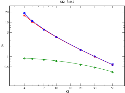
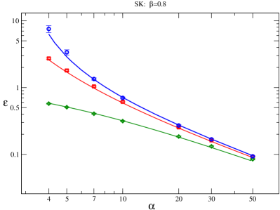
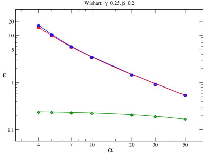
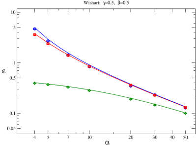
12 Numerical Results

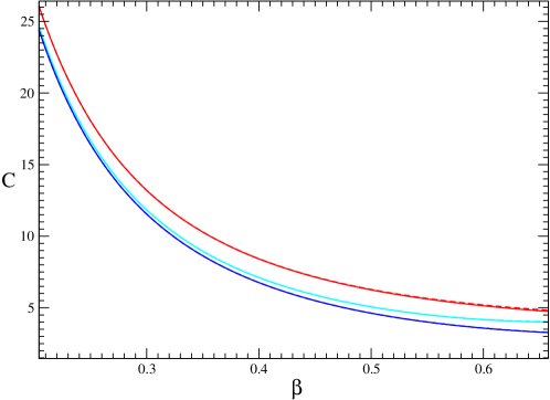
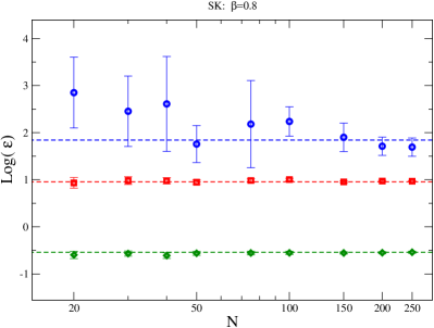
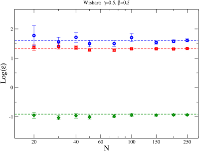
In the previous Sections we saw that the error of any algorithm that infers the network couplings by minimizing a cost function of the kind (13) satisfies (22), in the large $N$ limit, when the cavity arguments apply. The order parameters are the ones extremizing the free energy (20). For pseudo–likelihood maximization, the set of equations (84) for the order parameters has to be solved numerically, whereas for the local optimal and MF–ML estimators we computed analytically the error in the form, respectively, (30) and (60). Note that the error (22) is expressed in terms of three parameters that depend on the distribution of the teacher couplings: $Y$, $V$ and the trace of the inverse correlation matrix $\bm{C}$. As an example, we considered the the Gaussian ensemble of the SK model, with parameters given by $Y=1$ and relation (23) and the Wishart ensamble of (55) with parameters given by $Y=\gamma$ and relations (54) and (56). Figure 1 compares the predicted error with the mean squared error that we get from simulations, as a function of $\alpha$. We show results for the pseudo–likelihood, local optimal and MF–ML algorithms applied to the SK and the Wishart model. We only report results for the high–temperature (paramagnetic) region, i.e. for $\beta<\beta_{c}$ where $\beta_{c}$ defines the onset of spin–glass ordering. In this region, we expect that on the one hand, the cavity arguments are exact and the other hand, the convergence of the spin simulations to the thermal equilibrium is sufficiently fast. For the SK model, we have $\beta_{c}=1$ and for the Wishart model $\beta_{c}\simeq 1/(1+\sqrt{\gamma})$ for zero magnetization and small $q$ [36], where $q$ is the Edwards-Anderson order parameter. The data are generated by Monte Carlo sampling with a burn in time of $10^{7}N$ spin updates and sampling every $10\,N$ updates, and the couplings are recovered either by minimizing the pseudo–likelihood cost function (5) using a Newton method or from the empirical correlation matrices: see (26, 29) for the local optimal algorithm and (52) for MF–ML. The plot shows that the replica calculation predicts rather well the results of the simulations for systems of $N=100$ spins. In addiction, it is clear that the optimal local algorithm outperforms the other two methods and, in the high–temperature regime considered here, the MF–ML algorithm performs better than pseudo–likelihood maximization. This performance difference is more relevant for increasing $\beta$ and in the small $\alpha$ region, whereas it is almost negligible for large $\alpha$, in agreement with the asymptotic expansions. Finally, we compare the analytical results for the asymptotic behavior of the error computed in Section 11 with the results from simulations. Assuming the scaling (61), we fitted the function $\varepsilon=c/\alpha$ to the mean squared error of the couplings inferred from simulations at large $\alpha$. In Table 1 we show that this ’experimental’ value of $c$ is consistent with $c_{\mbox{\tiny{PLM}}}$ (62) and $c_{\mbox{\tiny{OPT}}}=c_{\mbox{\tiny{MF--ML}}}$ (63, 64). We then plot the predicted value of $c$ as a function of $\beta$ in Figure 2, where we can see that the difference between pseudo–likelihood maximization, the local optimal and MF–ML algorithms is almost indistinguishable and goes to zero for small $\beta$, as we would expect by noticing that the analytical formula for $c_{\mbox{\tiny{PLM}}}$ (62) agrees with $c_{\mbox{\tiny{OPT}}}=c_{\mbox{\tiny{MF--ML}}}$ (63, 64) up to second order in $\beta$. From the plot it is also clear that for larger $\beta$ –i.e. smaller stochasticity of the spins– the error in predicting the couplings is smaller.

The three algorithms show different behaviors in the small $\alpha$ region. As the MF–ML algorithm relies on the inversion of the correlation matrix (52), that becomes singular at $\alpha=1$, its error diverges at $\alpha=1$, as can be seen from (60). On the contrary, the error of the optimal local algorithm shows no divergence, since $\eta_{\mbox{\tiny{opt}}}=0$ and $\varepsilon=Y$ at $\alpha=1$ (see 29, 30). From simulations we also observe that the error of the pseudo–likelihood estimator increases for decreasing $\alpha$ and for $\alpha<2$ it reaches large values, with large variations across trials, while the extremization of the free energy (see 84) fails in the region $\alpha<2$. A way to overcome this divergence is to introduce a regularizing term in the objective function. We postpone the study of regularized estimators to future work. We present additional plots in Appendix G, showing the error dependence on the system size.

Figure 1: The mean squared error of the couplings inferred by using the pseudo–likelihood algorithm (blue dots), the optimal local algorithm (green dots) and the MF–ML algorithm (red dots) is compared to the corresponding average prediction error from the replica calculation (continuous lines). The error is plotted as a function of $\alpha$. Four different systems are considered: SK model at $\beta=0.2$ (top left), SK model at $\beta=0.8$ (top right), Wishart model with $\gamma=0.25$ at $\beta=0.2$ (bottom left) and Wishart model with $\gamma=0.5$ at $\beta=0.5$ (bottom right). The algorithms were tested on a system of $N=100$ spins and the results are averaged over $5$ realizations of the network and $100$ different datasets generated from each network. Error bars represent standard deviations of the means.

Figure 2: The values $c_{\mbox{\tiny{PLM}}}$ (62) for pseudo–likelihood maximization (dotted lines) and $c_{\mbox{\tiny{MF--ML}}}$ (64) for the MF–ML algorithm (continuous lines) are plotted as a function of $\beta$. The red lines correspond to the SK model, the blue lines to the Hopfield model with parameter $\gamma=0.25$ (light blue) and $\gamma=0.15$ (dark blue).

Model	Algorithm	c	c (simulations)
SK	PLM	$5.199$	$5.16\pm 0.04$
	MF–ML	$5.137$	$5.14\pm 0.05$
Wishart	PLM	$3.582$	$3.64\pm 0.06$
	MF–ML	$3.578$	$3.60\pm 0.05$

Table 1: The values of $c_{\mbox{\tiny{PLM}}}$ (62) for pseudo–likelihood maximization and $c_{\mbox{\tiny{MF--ML}}}$ (64) for the MF–ML algorithm are compared to the results ’c (simulations)’ we obtained by fitting the function $\varepsilon=c/\alpha$ to the mean squared error $\varepsilon$ of the inferred couplings obtained from simulations at large $\alpha$. We considered two systems: SK model at $\beta=0.6$ and Hopfield model with $\gamma=0.15$ at $\beta=0.6$. The algorithms were tested on a system of $N=200$ spins for $\alpha=900,950,1000$ and the results are averaged over $5$ realizations of the network and $10$ different datasets generated from each network.

13 Discussion and outlook

We have presented a statistical physics approach for calculating the reconstruction error of algorithms for learning the couplings of large Ising models. Our method assumes local cost functions for learning and is based on a combination of the replica trick and of cavity arguments for computing quenched averages over spin configurations which are drawn at random from a teacher network. A replica symmetric ansatz seems to be justified as long as the learning algorithms are based on convex cost functions. The cavity approach assumes a large densely connected network with couplings that are roughly of the same size leading to only weakly correlated spins. These assumptions are correct in the thermodynamic limit for certain statistical ensembles of network couplings but may also give good approximations for realistic networks. While our method is so far restricted to problems which are realisable by pairwise spin–interactions, it could nevertheless be of practical interest in providing approximate statistics for hypotheses testing against more complicated network models (having e.g. 3–spin interactions).

Our results show that the learning problem is, at least within our framework, surprisingly simple: An explicit estimator based on a quadratic cost function achieves minimal error and outperforms the more complicated pseudo–likelihood estimator. This optimal estimator only requires prior knowledge of the length of the true coupling vector. Moreover, a simple (symmetric) mean field approximation to the maximum likelihood estimator is asymptotically optimal and can be computed without such prior knowledge. In the case of the SK model, the region of small $\beta$ in which these results hold covers the entire paramagnetic phase, where our simple cavity arguments are known to be valid. It would be interesting to work out analytically how well the mean field estimator approximates the exact maximum likelihood estimator in the thermodynamic limit.

Our work is only a first step to an understanding of the typical performance of learning algorithms for the inverse Ising problem. From a technical point of view our method could be generalised in several directions. We have restricted ourselves to models where data are sampled from the paramagnetic phase of a teacher network. While it is possible to generalise the analysis, the average over samples from a spin–glass phase would usually require more complex types of cavity arguments [37] which are related to the breaking of the replica symmetry of the teacher network. In such a case, the simple Gaussian distribution of cavity fields on which our analysis strongly relies is no longer valid. One might expect that now the quadratic cost functions may no longer be optimal (and not even consistent) but could be outperformed by a pseudo–likelihood method.

We also expect that our cavity framework could be extended to sparse networks as long as the number of nonzero couplings per spin is large enough to allow for the application of the central limit arguments used in our work.

After finishing our work we became aware of a recent preprint [30] where similar learning problems (focussing on a teacher model with independent Gaussian couplings) were studied. The author applied a double replica calculation (the other set of replica are used for dealing with the partition function in the quenched average over the spins) instead of using cavity arguments. This results in a free energy function which agrees essentially with our result (20). However, the order parameters appearing in the free energy are not defined by (19) but by (7) instead, and the reconstruction error differs from ours. The major difference is that the result for the error in [30] does not contain the spin–correlation matrix as in our equation (22). We believe that this could be related to an implicit approximation of the correlation matrix by a unit matrix.

Appendix A Details of the replica calculation

From (11-12-18) one can see that the free energy can be written as

$$\begin{split}F=-\lim_{n\to 0}N^{-1}\nu^{-1}\frac{\partial}{\partial n}\ln&\int\prod_{a=1}^{n}\;d\bm{W}^{a}\left\{\sum_{\sigma_{0}}\int\,dh_{*}\prod_{a=1}^{n}dh_{a}\frac{1}{Z_{0}}\exp\left[\beta\sigma_{0}h_{*}\right]\right.\\ &\left.\exp\left[-\nu\sum_{a=1}^{n}\Phi(\sigma_{0}h_{a})\right]\;p_{\mbox{\tiny{cav}}}(h_{*},h_{1},\ldots h_{n})\right\}^{\alpha N},\end{split}$$ (70)

where $p_{\mbox{\tiny{cav}}}(h_{*},h_{1},\ldots h_{n})$ is a multivariate Gaussian density with zero mean and covariance given by (17). The average over the Gaussian fields yields quadratic terms in $\bm{W}^{*}$ and $\{\bm{W}^{a}\}_{a=1}^{n}$, that can be simplified by introducing the order parameters $\{R,q,q_{0}\}$ (19), that have to be defined via integrals over delta functions. One finds that free energy decouples into two terms:

$${F}(R,q,q_{0})=F_{0}(R,q,q_{0})+F_{1}(R,q,q_{0}).$$ (71)

The first one contains the integrals over the couplings and measures the density of the networks with order parameters $R,q,q_{0}$ :

$$F_{0}(R,q,q_{0})=-\lim_{n\to 0}\nu^{-1}\frac{\partial}{\partial n}\frac{1}{N}\ln Z_{\tiny{\mbox{coup}}},$$ (72)

with

$$\begin{split}Z_{\tiny{\mbox{coup}}}&=\int\prod_{a}d\bm{W^{a}}\prod_{a}\delta\left(\sum_{ij}W^{a}_{i}C_{ij}W^{*}_{j}-NR\right)\\ &\prod_{a}\delta\left(\sum_{ij}W^{a}_{i}C_{ij}W^{a}_{j}-Nq_{0}\right)\prod_{a<b}\delta\left(\sum_{ij}W^{a}_{i}C_{ij}W^{b}_{j}-Nq\right).\\ \end{split}$$ (73)

For notational simplicity here we have dropped the ’$0$’ from the correlation matrix $\bm{C}^{\backslash 0}$. $F_{0}$ can be computed following our derivation in [18]: we introduce the orthogonal matrix $\bm{U}$ that diagonalizes $\bm{C}=\bm{U}^{\top}\Lambda\bm{U}$,

$$\begin{split}Z_{\tiny{\mbox{coup}}}&=\int\prod_{a}d\bm{W^{a}}\prod_{a}\delta(\sum_{ijk}U_{ij}W^{a}_{j}\Lambda_{i}U_{ik}W^{*}_{k}-NR)\\ &\prod_{a}\delta(\sum_{ijk}U_{ij}W^{a}_{j}\Lambda_{i}U_{ik}W^{a}_{k}-Nq_{0})\prod_{a<b}\delta(\sum_{ijk}U_{ij}W^{a}_{j}\Lambda_{i}U_{ik}W^{b}_{k}-Nq),\\ \end{split}$$ (74)

and transform the student coupling vector into new variables $\bm{U}^{\top}\bm{W}^{a}\to\bm{W}^{a}$, which we give the same name. We then express the delta functions as integrals over the auxiliary parameters $\{\hat{R},\hat{q},\hat{q_{0}}\}$. The integration gives

$$\begin{split}F_{0}(R,q,q_{0})=\underset{\hat{R},\hat{q},\hat{q_{0}}}{\mbox{extr}}\;\frac{1}{\nu}&\left\{i\hat{q_{0}}q_{0}+i\hat{R}R-\frac{i}{2}\hat{q}q+\frac{1}{2N}\sum_{i}\frac{\hat{q}+i\hat{R}^{2}(\sum_{j}U_{ij}W^{*}_{j})^{2}\Lambda_{i}}{2\hat{q_{0}}-\hat{q}}\right.\\ &\left.+\frac{1}{2N}\sum_{i}\ln\left[\Lambda_{i}(i\hat{q}-2i\hat{q_{0}})\right]-\frac{1}{2}\ln(2\pi)\right\}\end{split}$$ (75)

and the extremum over the conjugate order parameters yields

$$F_{0}(R,q,q_{0})=\frac{1}{2\nu}\left[\frac{q_{0}-R^{2}/V}{q-q_{0}}-\ln(q_{0}-q)+\frac{1}{N}Tr\ln\overline{C}\right],$$ (76)

where $V$, representing the cavity variance of the teacher field $h_{*}$, was introduced in (19). The second term of (71) contains the integration over the cavity fields $h_{*}$ and $\{h_{a}\}_{a=1}^{n}$:

$$\begin{split}F_{1}(R,q,q_{0})=-\lim_{n\to 0}N^{-1}\nu^{-1}\frac{\partial}{\partial n}\ln&\left\{2\int\,dh_{*}\prod_{a=1}^{n}dh_{a}\frac{1}{Z_{0}}\exp\left[\beta h_{*}\right]\right.\\ \exp\left[-\nu\sum_{a=1}^{n}\Phi(h_{a})\right]\;&\left.p_{\mbox{\tiny{cav}}}(h_{*},h_{1},\ldots h_{n})\right\}^{\alpha N},\end{split}$$ (77)

where we applied the change of variables $\sigma_{0}h_{*}\to h_{*}$ and $\sigma_{0}h_{a}\to h_{a}$. The integration gives

$$\begin{split}F_{1}(R,q,q_{0})=&-\frac{\alpha}{\nu}\int\frac{dv}{\sqrt{2\pi q}}\;e^{-\frac{(v-\beta R)^{2}}{2q}}\;\ln\int\frac{dy}{\sqrt{2\pi(q_{0}-q)}}\;e^{-\frac{(y-v)^{2}}{2(q_{0}-q)}}e^{-\nu\Phi(y)}.\end{split}$$ (78)

Hence the free energy (71) becomes

$$\begin{split}{F}(R,q,q_{0})=-&\frac{1}{\nu}\left\{\frac{1}{2}\frac{q_{0}-R^{2}/V}{q_{0}-q}+\frac{1}{2}\ln(q_{0}-q)-\frac{1}{2N}Tr\ln\overline{C}\right.\\ &\left.+\alpha\int dv\;G_{\beta R,q}(v)\;\ln\int dy\;G_{v,q_{0}-q}(y)e^{-\nu\Phi(y)}\right\},\end{split}$$ (79)

where $G_{\mu,\omega}(v)$ denotes a scalar Gaussian density with mean $\mu$ and standard deviation $\omega$.

Appendix B Saddle point equations for the order parameters

We rewrite (20) as

$$F=-\underset{q,R,x}{\mbox{extr}}\,\left\{\frac{1}{2}\frac{q-R^{2}/V}{x}+\alpha\int\mathcal{D}v\;\max_{y}\left[-\frac{(y-\sqrt{q}v-\beta R)^{2}}{2x}-\Phi(y)\right]\right\},$$ (80)

where $\mathcal{D}v=e^{-v^{2}/2}/\sqrt{2\pi}$. The extremum over the order parameters gives the following set of equations:

$$\begin{split}&0=\frac{1}{x}-\frac{\alpha}{\sqrt{q}}\int\mathcal{D}v\;v\;\left.\frac{\partial\Phi(y)}{\partial y}\right|_{y=\hat{y}}\\ &0=-\frac{R}{Vx}-\alpha\beta\int\mathcal{D}v\;\left.\frac{\partial\Phi(y)}{\partial y}\right|_{y=\hat{y}}\\ &0=-\frac{1}{x^{2}}\left(q-\frac{R^{2}}{V}\right)+\alpha\int\mathcal{D}v\;\left(\left.\frac{\partial\Phi(y)}{\partial y}\right|_{y=\hat{y}}\right)^{2},\end{split}$$ (81)

where

$$\hat{y}=\mbox{arg}\max_{y}\left[-\frac{(y-\sqrt{q}v-\beta R)^{2}}{2x}-\Phi(y)\right].$$ (82)

If we consider the pseudo–likelihood algorithm with $\Phi(y)=-\beta y+\ln 2\cosh(\beta y)$ (see the the definition of $\Phi$ (13) and the cost function (5)) we obtain the following equations for the order parameters:

$$0=\frac{1}{x}+\frac{\alpha\beta}{\sqrt{q}}\int\mathcal{D}v\;v\;\left(1-\tanh(\beta\hat{y})\right)$$ (83a)

$$0=-\frac{R}{Vx}+\alpha\beta^{2}\int\mathcal{D}v\left(1-\tanh(\beta\hat{y})\right)$$ (83b)

$$0=-\frac{1}{x^{2}}\left(q-\frac{R^{2}}{V}\right)+\alpha\beta^{2}\int\mathcal{D}v\;\left(1-\tanh(\beta\hat{y})\right)^{2},$$ (83c)

where $\hat{y}$ is defined by

$$\hat{y}=\sqrt{q}v+\beta R+\beta x(1-\tanh(\beta\hat{y})).$$ (84)

Appendix C Relation between order parameters

We introduce the auxiliary variables $\{\eta_{1},\eta_{2}\}$ in the free energy $F=F_{0}+F_{1}$ as follows:

$$\begin{split}F_{0}(R,q,q_{0},\eta_{1},\eta_{2})&=-\lim_{n\to 0}\nu^{-1}N^{-1}\frac{\partial}{\partial n}\ln\int\prod_{a}d\bm{W^{a}}\;d\hat{q_{0}}\;d\hat{R}\;d\hat{q}\\ &\prod_{a}e^{i\hat{R}(\sum_{ijk}U_{ij}W^{a}_{j}(\Lambda_{i}+\eta_{1})U_{ik}W^{*}_{k}-NR)}\prod_{a}e^{i\hat{q_{0}}(\sum_{ijk}U_{ij}W^{a}_{j}\Lambda_{i}U_{ik}W^{a}_{k}-Nq_{0})}\\ &\prod_{a<b}e^{i\hat{q}(\sum_{ijk}U_{ij}W^{a}_{j}(\Lambda_{i}+\eta_{2})U_{ik}W^{b}_{k}-Nq)}.\end{split}$$ (85)

The integration gives

$$\begin{split}F_{0}(R,q,q_{0},\eta_{1},\eta_{2})=&\underset{\hat{R},\hat{q},\hat{q_{0}}}{\mbox{extr}}\;\frac{1}{\nu}\left\{i\hat{q_{0}}q_{0}+i\hat{R}R-\frac{i}{2}\hat{q}q\right.\\ &\left.+\frac{1}{2N}\sum_{i}\frac{\hat{q}(\Lambda_{i}+\eta_{2})+i\hat{R}^{2}(\sum_{j}U_{ij}W^{*}_{j})^{2}(\Lambda_{i}+\eta_{1})^{2}}{2\hat{q_{0}}-\hat{q}(\Lambda_{i}+\eta_{2})}\right.\\ &\left.+\frac{1}{2N}\sum_{i}\ln\left[i\hat{q}(\Lambda_{i}+\eta_{2})-2i\hat{q_{0}}\right]-\frac{1}{2}\ln(2\pi)\right\}.\end{split}$$ (86)

From (85) it is easy to see that the parameters $\{\rho,Q\}$ can be derived by derivatives of the free energy:

$$\begin{split}&\rho=N^{-1}\overline{\bm{W^{*}}\cdot\langle\bm{W}\rangle}=\frac{\nu}{i\hat{R}}\frac{\partial F_{0}}{\partial\eta_{1}},\\ &Q=N^{-1}\overline{\langle\bm{W}\rangle^{2}}=-\frac{2\nu}{i\hat{q}}\frac{\partial F_{0}}{\partial\eta_{2}}\end{split}$$ (87)

in the limit $\{\eta_{1}\to 0,\eta_{2}\to 0\}$, where $\hat{R}$ and $\hat{q}$ are the values extremizing (86) in the limit $\{\eta_{1}\to 0,\eta_{2}\to 0\}$:

$$\begin{split}&\hat{q}=i\frac{R^{2}-Vq}{V(q_{0}-q)^{2}},\\ &\hat{R}=i\frac{R}{V(q-q_{0})},\\ &\hat{q_{0}}=i\frac{R^{2}+V(q_{0}-2q)}{2V(q_{0}-q)^{2}}.\end{split}$$ (88)

From (86), (87) and (88) we recover (21).

Appendix D Replica result for quadratic cost functions

If the cost function has the simple quadratic form (27), computing the maximum and the integrals in (20) can be done analytically and the free energy is

$$F=-\frac{q-R^{2}/V}{2x}+\alpha\frac{q+\beta R(\beta R-2\eta)-\eta^{2}x}{2(1+x)},$$ (89)

where the order parameters obey to the following saddle point equations:

$$\begin{split}&q=\frac{\eta^{2}(1+\alpha\beta^{2}V)}{(\alpha-1)(1+\beta^{2}V)},\\ &R=\frac{\eta\beta V}{1+\beta^{2}V},\\ &x=\frac{1}{(\alpha-1)}.\end{split}$$ (90)

With this result, the reconstruction error (22) for the linear estimator becomes (28). Moreover, we can compute the parameter $\Delta$ defined in (33) as follows. If the ’training energy’ per degree of freedom $N$ becomes self–averaging we can use the relation (see also (11))

$$E(\bm{W}^{ML})=-\lim_{\nu\to\infty}\nu^{-1}\ln Z$$ (91)

to explicitly evaluate the minimum training energy as

$$E(\bm{W}^{ML})=\frac{N}{\alpha}F(\bm{W}^{ML})=-\frac{N\eta^{2}}{2\alpha}\frac{(1+\alpha\beta^{2}V)}{(1+\beta^{2}V)},$$ (92)

where the second equality follows from (89) with the order parameters fixed to their saddle point values (90). From (32) and (92), one finds (34).

Appendix E Asymptotics from the replica approach

In the large $\alpha$ limit, we know that the parameter $x$ gets small and the parameters $q$ and $R$ both converge to $V$. For the pseudo–likelihood estimator we find the following relation, starting from (83b) in the limit $R\to V$ and (83c):

$$q-\frac{R^{2}}{V}=\frac{1}{\alpha\beta^{2}}\frac{\int\mathcal{D}v\;\left(1-\tanh(\beta\hat{y})\right)^{2}}{\left[\int\mathcal{D}v\left(1-\tanh(\beta\hat{y})\right)\right]^{2}}$$ (93)

where $\hat{y}$ is given by (84), that in the limit of small $x$ becomes $\hat{y}\simeq\sqrt{q}v+\beta R$. Via a change of variable, we find the following result in the limit $R\to V,q\to V$:

$$\begin{split}q-\frac{R^{2}}{V}&=\frac{1}{\alpha\beta^{2}}\frac{\int dv\;G_{\beta V,V}(v)\left(1-\tanh(\beta v)\right)^{2}}{\left[\int dv\;G_{\beta V,V}(v)\left(1-\tanh(\beta v)\right)\right]^{2}}\\ &\simeq\frac{1}{\alpha\beta^{2}}\frac{1}{\int dv\;G_{\beta V,V}(v)\left(1-\tanh^{2}(\beta v)\right)},\end{split}$$ (94)

where in the last equality we exploited the relation $\int dv\;G_{\beta V,V}(v)\tanh(\beta v)=\int dv\;G_{\beta V,V}(v)\tanh^{2}(\beta v)$. Hence, the error (22) for large $\alpha$ scales as

$$\varepsilon\simeq\left(q-\frac{R^{2}}{V}\right)\frac{1}{N}\mbox{Tr}\overline{C^{-1}}\simeq\frac{1}{\alpha\beta^{2}}\frac{1}{\int dv\;G_{\beta V,V}(v)\left(1-\tanh^{2}(\beta v)\right)}\;\frac{1}{N}\mbox{Tr}\overline{C^{-1}}.$$ (95)

Appendix F Asymptotic error for pseudo–likelihood estimator

We show that $U_{ij}=-B_{ij}$ for the pseudo–likelihood case assuming that the model is matched to the true data generating distribution. We start from the relations

$$U_{ij}=\sum_{\bm{\sigma}_{\setminus 0}}P(\bm{\sigma}_{\setminus 0})\sum_{\sigma_{0}}P(\sigma_{0}|\bm{\sigma}_{\setminus 0})\partial_{i}\partial_{j}\ln P(\sigma_{0}|\bm{\sigma}_{\setminus 0})$$ (96)

and

$$B_{ij}=\sum_{\bm{\sigma}_{\setminus 0}}P(\bm{\sigma}_{\setminus 0})\sum_{\sigma_{0}}P(\sigma_{0}|\bm{\sigma}_{\setminus 0})\partial_{i}\ln P(\sigma_{0}|\bm{\sigma}_{\setminus 0})\partial_{j}\ln P(\sigma_{0}|\bm{\sigma}_{\setminus 0}).$$ (97)

We next perform the inner expectation over $P(\sigma_{0}|\bm{\sigma}_{\setminus 0})$. The result follows from

$$\partial_{i}\partial_{j}\ln P=-\partial_{i}\ln P\;\partial_{j}\ln P+\frac{1}{P}\partial_{i}\partial_{j}P$$

and the fact that, by normalisation of $P$, one gets $\sum_{\sigma}\partial_{i}\partial_{j}P(\sigma|\bm{\sigma}_{\setminus 0})=0$.

Appendix G Error dependence on the system size

Figure 3: Mean squared error of the couplings inferred by using the pseudo–likelihood algorithm (blue dots) the optimal local algorithm (green dots) and the MF–ML algorithm (red dots) as a function of the system size $N$, for fixed $\alpha=5$. The dotted lines represent replica results. Two different systems are considered: SK model at $\beta=0.8$ (left) and Wishart model with $\gamma=0.5$ at $\beta=0.5$ (right). The results are averaged over $5$ realizations of the network and $20$ different datasets generated from each network. Error bars represent standard deviations of the means.

In Figure 1 we showed that the reconstruction error in systems with $N=100$ spins well agrees with the replica result, which is valid in the thermodynamic limit. However, it is relevant for applications to show an example of how the system size can affect the reconstruction error. In Figure 3 we show results obtained by fixing $\alpha$ and varying $N$. First of all we notice that finite size effects are much stronger for the the pseudo–likelihood algorithm than for the other two methods. Moreover, while the optimal local estimator always seems to outperform the other two methods, the performance difference between MF–ML and pseudo–likelihood algorithms depends more strongly on the system parameters ($\alpha$, $\beta$, teacher coupling distribution), if $N$ is small. For instance, we see in Figure 3 that, for systems of $N=20,30$ spins with couplings drawn from the Wishart distribution, the error of the MF–ML and pseudo–likelihood algorithms are compatible.

References

- [1] Schneidman, E., Berry, M. J., Segev, R., and Bialek, W.: Weak pairwise correlations imply strongly correlated network states in a neural population. Nature 440, 1007–1012 (2006)
- [2] Roudi, Y., Tyrcha, J., and Hertz, J.: Ising model for neural data: model quality and approximate methods for extracting functional connectivity. Physical Review E 79, 051915 (2009)
- [3] Weigt, M., White, R. A., Szurmant, H., Hoch, J. A., and Hwa, T.: Identification of direct residue contacts in protein–protein interaction by message passing. Proceedings of the National Academy of Sciences 106, 67–72 (2009)
- [4] Lezon, T. R., Banavar, J. R., Cieplak, M., Maritan, A., and Fedoroff, N. V.: Using the principle of entropy maximization to infer genetic interaction networks from gene expression patterns. Proceedings of the National Academy of Sciences 103, 19033–19038 (2006)
- [5] Broderick, T., Dudik, M., Tkacik, G., Schapire, R. E., and Bialek, W.: Faster solutions of the inverse pairwise Ising problem. ArXiv e-prints (2007)
- [6] Kappen, H. J. and Rodríguez, F. d. B.: Efficient learning in Boltzmann machines using linear response theory. Neural Computation 10, 1137–1156 (1998)
- [7] Tanaka, T.: Mean-field theory of Boltzmann machine learning. Physical Review E 58, 2302 (1998)
- [8] Roudi, Y., Aurell, E., and Hertz, J.: Statistical physics of pairwise probability models. Frontiers in Computational Neuroscience 3, 22 (2009)
- [9] Sessak, V. and Monasson, R.: Small-correlation expansions for the inverse Ising problem. Journal of Physics A: Mathematical and Theoretical 42, 055001 (2009)
- [10] Besag, J.: Spatial interaction and the statistical analysis of lattice systems. Journal of the Royal Statistical Society Series B (Methodological) 192–236 (1974)
- [11] Aurell, E. and Ekeberg, M.: Inverse Ising inference using all the data. Physical review letters 108, 090201 (2012)
- [12] Decelle, A. and Ricci-Tersenghi, F.: Pseudolikelihood decimation algorithm improving the inference of the interaction network in a general class of ising models. Physical review letters 112, 070603 (2014)
- [13] Mozeika, A., Dikmen, O., and Piili, J.: Consistent inference of a general model using the pseudolikelihood method. Physical Review E 90, 010101 (2014)
- [14] Tyagi, P., Marruzzo, A., Pagnani, A., Antenucci, F., and Leuzzi, L.: Regularization and decimation pseudolikelihood approaches to statistical inference in X Y spin models. Physical Review B 94, 024203 (2016)
- [15] Opper, M. and Kinzel, W.: Statistical mechanics of generalization. In Models of neural networks III, 151–209. Springer (1996)
- [16] Engel, A. and Van den Broeck, C.: Statistical mechanics of learning. Cambridge University Press (2001)
- [17] Nishimori, H.: Statistical physics of spin glasses and information processing: an introduction, vol. 111. Clarendon Press (2001)
- [18] Bachschmid-Romano, L. and Opper, M.: Learning of couplings for random asymmetric kinetic Ising models revisited: random correlation matrices and learning curves. Journal of Statistical Mechanics: Theory and Experiment 2015, P09016 (2015)
- [19] Mézard, M., Parisi, G., and Virasoro, M.: Spin glass theory and beyond: An Introduction to the Replica Method and Its Applications, vol. 9. World Scientific Publishing Co Inc (1987)
- [20] Schervish, M. J.: Theory of statistics. Springer Science & Business Media (2012)
- [21] Cocco, S. and Monasson, R.: Adaptive cluster expansion for inferring Boltzmann machines with noisy data. Physical review letters 106, 090601 (2011)
- [22] Sohl-Dickstein, J., Battaglino, P. B., and DeWeese, M. R.: New method for parameter estimation in probabilistic models: minimum probability flow. Physical review letters 107, 220601 (2011)
- [23] Ricci-Tersenghi, F.: The Bethe approximation for solving the inverse Ising problem: a comparison with other inference methods. Journal of Statistical Mechanics: Theory and Experiment 2012, P08015 (2012)
- [24] Nguyen, H. C. and Berg, J.: Bethe–Peierls approximation and the inverse Ising problem. Journal of Statistical Mechanics: Theory and Experiment 2012, P03004 (2012)
- [25] Seung, H., Sompolinsky, H., and Tishby, N.: Statistical mechanics of learning from examples. Physical Review A 45, 6056 (1992)
- [26] Sherrington, D. and Kirkpatrick, S.: Solvable model of a spin-glass. Physical review letters 35, 1792 (1975)
- [27] Bray, A. and Moore, M.: Metastable states in spin glasses. Journal of Physics C: Solid State Physics 13, L469 (1980)
- [28] Kinouchi, O. and Caticha, N.: Optimal generalization in perceptions. Journal of Physics A: mathematical and General 25, 6243 (1992)
- [29] Advani, M. and Ganguli, S.: Statistical mechanics of optimal convex inference in high dimensions. Physical Review X 6, 031034 (2016)
- [30] Berg, J.: Statistical mechanics of the inverse Ising problem and the optimal objective function. ArXiv e-prints (2016)
- [31] Opper, M. and Winther, O.: Adaptive and self-averaging Thouless-Anderson-Palmer mean-field theory for probabilistic modeling. Physical Review E 64, 056131 (2001)
- [32] Hopfield, J. J.: Neural networks and physical systems with emergent collective computational abilities. Proceedings of the national academy of sciences 79, 2554–2558 (1982)
- [33] Parisi, G. and Potters, M.: Mean-field equations for spin models with orthogonal interaction matrices. Journal of Physics A: Mathematical and General 28, 5267 (1995)
- [34] Opper, M., Cakmak, B., and Winther, O.: A theory of solving TAP equations for Ising models with general invariant random matrices. Journal of Physics A: Mathematical and Theoretical 49, 114002 (2016)
- [35] Abadir, K. M. and Magnus, J. R.: Matrix Algebra. Cambridge University Press (2005)
- [36] Amit, D. J., Gutfreund, H., and Sompolinsky, H.: Storing infinite numbers of patterns in a spin-glass model of neural networks. Physical Review Letters 55, 1530 (1985)
- [37] Mézard, M. and Parisi, G.: The Bethe lattice spin glass revisited. European Physical Journal B 20, 217–233 (2001)