Anharmonic interatomic force constants and thermal conductivity from Grüneisen parameters: an application to graphene

Abstract

Phonon-mediated thermal conductivity, which is of great technological relevance, fundamentally arises due to anharmonic scattering from interatomic potentials. Despite its prevalence, accurate first-principles calculations of thermal conductivity remain challenging, primarily due to the high computational cost of anharmonic interatomic force constant (IFCs) calculations. Meanwhile, the related anharmonic phenomenon of thermal expansion is much more tractable, being computable from the Grüneisen parameters associated with phonon frequency shifts due to crystal deformations. In this work, we propose a novel approach for computing the largest cubic IFCs from the Grüneisen parameter data. This allows an approximate determination of the thermal conductivity via a much less expensive route. The key insight is that although the Grüneisen parameters cannot possibly contain all the information on the cubic IFCs, being derivable from spatially uniform deformations, they can still unambiguously and accurately determine the largest and most physically relevant ones. By fitting the anisotropic Grüneisen parameter data along judiciously designed deformations, we can deduce (i.e., reverse engineer) the dominant cubic IFCs and estimate three-phonon scattering amplitudes. We illustrate our approach by explicitly computing the largest cubic IFCs and thermal conductivity of graphene, especially for its out-of-plane (flexural) modes that exhibit anomalously large anharmonic shifts and thermal conductivity contributions. Our calculations on graphene not only exhibits reasonable agreement with established density-functional theory results, but also presents a pedagogical opportunity for introducing an elegant analytic treatment of the Grüneisen parameters of generic two-band models. Our approach can be readily extended to more complicated crystalline materials with nontrivial anharmonic lattice effects.

I Introduction

The harmonic approximation is ubiquitous in physics and engineering Born and Huang (1956); Maradudin et al. (1965). Based on the Taylor expansion about an equilibrium, it describes the leading-order oscillatory physics in extremely diverse settingsMaradudin et al. (1965); Horton and Maradudin (1974). Indeed, in much of condensed matter physics and materials engineering, it plays a fundamental role in describing vibrational degrees of freedom known as phonons, which underpins phenomena like acoustic behavior, infrared and Raman spectra, and superconductivityMaradudin et al. (1965). More recently, mechanical systems with harmonic elements have also been intensely investigated for their extremely experimentally accessible topological propertiesSalerno and Carusotto (2014); Nash et al. (2015); Wang et al. (2015); Süsstrunk and Huber (2015); Yang et al. (2015); Zhu et al. (2015); Fleury et al. (2015); Paulose et al. (2015); Ong and Lee (2016); Huber (2016); Liu et al. (2016); Lu et al. (2016); Lee et al. (2017).

However, there are also many important phenomena based on physics beyond the harmonic approximationLeibfried and Ludwig (1961); Horton and Maradudin (1974). Everyday-life observations like thermal expansion and conduction arise due to the anharmonicity of the interatomic potential, since a purely harmonic crystal with vanishing energy derivatives beyond the second order can neither expand nor dissipate. The performance of materials for heat dissipation, heat transport, thermal coating, and thermoelectric applications depends on the key quantity known as thermal conductivityBroido et al. (2005); Snyder and Toberer (2008); Ward et al. (2009); Garg et al. (2011); Zebarjadi et al. (2012); Broido et al. (2012). Indeed, the development of advanced technological applications like nanotube-based electronic devices require an accurate understanding of how phonon anharmonicity – intrinsic or artificially induced – affect their thermal performanceWang et al. (2007).

In view of the prevalence of anharmonicity in describing these diverse physical phenomena, various methods have been developed to calculate the third-order derivative of energy with respect to atomic displacements, i.e., the cubic IFCs or simply the cubic force constants (CFCs) of a crystal. We note that techniques to obtain the second-order derivatives of energy (or simply force constants) are well-developed, and include the supercell methodFrank et al. (1995); Kresse et al. (1995); Ackland et al. (1997); Parlinski et al. (1997); Alfè (2009); Gan et al. (2006, 2010); Liu et al. (2014); Togo and Tanaka (2015); Togo et al. (2015) and density-functional perturbation theory (DFPT)Baroni et al. (1987, 2001). The extension of the supercell methods to the third order has been carried out in the real spaceEsfarjani and Stokes (2008); Shiomi et al. (2011) or in reciprocal space using DFPTDebernardi et al. (1995); Ward et al. (2009); Paulatto et al. (2013) or compressed sensingZhou et al. (2014). Other methods include extracting CFCs from molecular dynamics simulationsHellman and Abrikosov (2013). Most of these methods for the computation of CFCs and hence thermal conductivity are computationally intensive, and it remains an open task to find more inexpensive approaches.

Meanwhile, there exists a useful measure of phonon anharmonicity known as the Grüneisen parameter that can be easily computed from first-principles without the explicit knowledge of the CFCs. This has been demonstrated in Refs. Pavone et al., 1993; Mounet and Marzari, 2005. Defined as the fractional change in phonon mode energy per fractional change in volume, it is directly related to the thermal expansion coefficient (TEC) and the specific heat capacity. Indeed, the determination of Grüneisen parameter has already provided an efficient determination of thermal expansion coefficients of orthorhombic systemsGan et al. (2015); Liu et al. (2017), a trigonal systemArnaud et al. (2016), and hexagonal systemsMounet and Marzari (2005); Ding and Xiao (2015); Gan and Liu (2016).

In this work, we introduce an approach for computing the most physically relevant CFCs, and hence a good approximation to the thermal conductivity, from anisotropic Grüneisen parameters corresponding to a set of strategically selected deformations. Such anisotropic Grüneisen parameters have been previously employed for the calculation of thermal expansion coefficientsGan et al. (2015); Gan and Liu (2016). Their computation requires only knowledge of how the phonon dispersions change under spatially uniform deformations, which are obtainable through standard phonon calculations. Our approach is much less expensive than a direct evaluation of third-order derivatives of energy with respect to displacements based on supercell methods or DFPT methods Michel et al. (2015), which involve meticulously keeping track of atomic displacements within the supercell.

Although the Grüneisen parameter data so obtained clearly contains less information than those of third-order DFPT, the key insight is that it is already sufficient for determining the largest few and hence most physically important CFCs and their counterparts related by symmetry. This can be systematically performed by “reverse engineering” the CFCs based on a general expression for the anisotropic Grüneisen parameter, to be derived in Section II, and the Grüneisen parameters data from phonon dispersions calculated using standard density-functional theory (DFT). We demonstrate the veracity of our approach by showing that the thermal conductivity of out-of-plane acoustic phonons for graphene computed from our CFCs agree fairly closely with established results.

The paper is structured as follows. We begin in Section II by developing a framework for describing crystal anharmonicity in terms of the anisotropic Grüneisen parameters, and showing how the CFCs contained therein affect thermal expansion and conduction. Next in Section III, we detail our recipe for recovering the dominant CFCs from Grüneisen parameter data obtained via simple DFT computations on deformed crystals. In Sect IV, we provide a pedagogical illustration of how our approach can be applied to compute the CFCs and thermal conductivity of the flexural modes of graphene.

II Anharmonicity in crystals

Consider a lattice of atoms interacting via a position-dependent potential energy

$$U= \frac{1}{2}\sum_{l,l^{\prime},j,j^{\prime}}\sum_{\alpha\beta}\Phi_{lj,l^{\prime}j^{\prime}}^{\alpha\beta}u^{\alpha}_{lj}u^{\beta}_{l^{\prime}j^{\prime}}$$

$$+\frac{1}{6}\sum_{l,l^{\prime}l^{\prime\prime},j,j^{\prime}j^{\prime\prime}}\sum_{\alpha\beta\gamma}\Psi_{lj,l^{\prime}j^{\prime},l^{\prime\prime}j^{\prime\prime}}^{\alpha\beta\gamma}u^{\alpha}_{lj}u^{\beta}_{l^{\prime}j^{\prime}}u^{\gamma}_{l^{\prime\prime}j^{\prime\prime}}$$

where $u^{\alpha}_{lj}$ is the $\alpha$th Cartesian direction of the displacement from equilibrium of the $j$th atom in the $l$th unit cell at ${\bm{R}}_{l}$. $U$ comprises harmonic energy penalties from the quadratic interatomic force constants $\Phi_{lj,l^{\prime}j^{\prime}}^{\alpha\beta}$, as well as anharmonic terms from the CFCs $\Psi_{lj,l^{\prime}j^{\prime},l^{\prime\prime}j^{\prime\prime}}^{\alpha\beta\gamma}$. Terms of quartic order can usually be neglected, except for specific materials with unusually large mean square atomic displacementsTadano and Tsuneyuki (2015). In general, $\Phi_{lj,l^{\prime}j^{\prime}}^{\alpha\beta}$ and $\Psi_{lj,l^{\prime}j^{\prime},l^{\prime\prime}j^{\prime\prime}}^{\alpha\beta\gamma}$ are not directly dependent on each other, other geometric relations exist between themLeibfried and Ludwig (1961). Due to translational invariance, we can define a dynamical matrix

$$D^{\alpha\beta}_{jj^{\prime}}({\bm{q}})=\frac{1}{\sqrt{M_{j}M_{j^{\prime}}}}\sum_{l^{\prime}}\frac{\partial^{2}U}{\partial u^{\alpha}_{0j}\partial u^{\beta}_{l^{\prime}j^{\prime}}}e^{i{\bm{q}}\cdot{\bm{R}}_{l^{\prime}}},$$ (2)

at a wave vector ${\bm{q}}$, whose squared eigenvalues $\omega_{{\bm{q}}s}^{2}$ describe the phonon dispersion of the $s$th phonon branch, where $M_{j}$ is the mass of the $j$th atom.

In the absence of anharmonicity, $\Phi^{\alpha\beta}_{lj,l^{\prime}j^{\prime}}$ is a constant that does not depend on the displacements $u^{\alpha}_{lj}$. In this case, then, the phonon dispersions are independent of any changes in the size or shape of the crystal, precluding thermal expansion due to energetic considerations. At the many-body level, the lack of higher order terms also precludes any scattering processes that lead to thermal resistivity.

As such, a realistic phonon potential must contain anharmonic terms. Below, we derive an expression for the anisotropic Grüneisen parameter based on first-order perturbation theory. For this, we need to investigate how the phonon frequency $\omega_{{\bm{q}}s}$ of wave vector ${\bm{q}}$ and mode index $s$ changes when the crystal is deformed according to the deformation matrix $E$ given by

$$E=\left(\begin{array}[]{ccc}e_{1}&e_{6}/2&e_{5}/2\\ e_{6}/2&e_{2}&e_{4}/2\\ e_{5}/2&e_{4}/2&e_{3}\end{array}\right)$$ (3)

with the six parameters $e_{i}$, $i=1,2,\cdots,6$ appearing as in the Voigt notationNye (1985).

Without loss of generality, we parametrize a small deformation as $e_{i}=\eta f_{i}$, $i=1,\cdots,6$, where $\eta$ is a small parameter and $f_{i}$ are constants normalized according to $\sum_{i}f_{i}^{2}=1$. Now $E=\eta F$ where

$$F=\left(\begin{array}[]{ccc}f_{1}&f_{6}/2&f_{5}/2\\ f_{6}/2&f_{2}&f_{4}/2\\ f_{5}/2&f_{4}/2&f_{3}\end{array}\right)$$ (4)

An infinitesimal strain $\eta F$ may result in a change in volume as atoms at equilibrium positions ${\bm{r}}$ are shifted to $(\mathit{I}+\eta F){\bm{r}}={\bm{r}}+\eta F{\bm{r}}$ where $\mathit{I}$ is the $3\times 3$ identity matrix. Since this displacement is much smaller than the lattice constant, the effect of anharmonicity and hence the Grüneisen parameter can be perturbatively treated around the equilibrium volume (i.e., $\eta=0$) as follows:

$$\gamma_{{\bm{q}}s}(F) = -\frac{1}{\omega_{{\bm{q}}s}}\frac{\partial\omega_{{\bm{q}}s}}{\partial\eta}=-\frac{1}{2\omega^{2}_{{\bm{q}}s}}\frac{\partial(\omega^{2}_{{\bm{q}}s})}{\partial\eta}=-\frac{1}{2\omega^{2}_{{\bm{q}}s}}\frac{\partial}{\partial\eta}\sum_{\alpha j,\beta j^{\prime}}[\epsilon_{{\bm{q}}s}^{\alpha j}]^{*}D^{\alpha\beta}_{jj^{\prime}}({\bm{q}})\epsilon_{{\bm{q}}s}^{\beta j^{\prime}}$$ (5)

$$= -\frac{1}{2\omega^{2}_{{\bm{q}}s}}\frac{\partial}{\partial\eta}\sum_{\alpha j,\beta j^{\prime}}[\epsilon_{{\bm{q}}s}^{\alpha j}]^{*}\left[\sum_{l^{\prime}}\frac{1}{\sqrt{M_{j}M_{j^{\prime}}}}e^{i{\bm{q}}\cdot{\bm{R}}_{l^{\prime}}}\frac{\partial^{2}U}{\partial u_{0j}^{\alpha}\partial u_{l^{\prime}j^{\prime}}^{\beta}}\right]\epsilon_{{\bm{q}}s}^{\beta j^{\prime}}$$

$$= -\frac{1}{2\omega^{2}_{{\bm{q}}s}}\frac{\partial}{\partial\eta}\sum_{\alpha j,\beta j^{\prime}}[\epsilon_{{\bm{q}}s}^{\alpha j}]^{*}\left[\sum_{l^{\prime}}\frac{1}{\sqrt{M_{j}M_{j^{\prime}}}}e^{i{\bm{q}}\cdot{\bm{R}}_{l^{\prime}}}\sum_{l^{\prime\prime}j^{\prime\prime}\gamma}\left(\Psi^{\alpha\beta\gamma}_{0j,l^{\prime}j^{\prime},l^{\prime\prime}j^{\prime\prime}}u_{l^{\prime\prime}j^{\prime\prime}}^{\gamma}\right)\right]\epsilon_{{\bm{q}}s}^{\beta j^{\prime}}$$

$$= -\frac{1}{2\omega^{2}_{{\bm{q}}s}}\sum_{\alpha j,\beta j^{\prime}}[\epsilon_{{\bm{q}}s}^{\alpha j}]^{*}\left[\sum_{l^{\prime}}\frac{1}{\sqrt{M_{j}M_{j^{\prime}}}}e^{i{\bm{q}}\cdot{\bm{R}}_{l^{\prime}}}\sum_{l^{\prime\prime}j^{\prime\prime}\gamma}\left(\Psi^{\alpha\beta\gamma}_{0j,l^{\prime}j^{\prime},l^{\prime\prime}j^{\prime\prime}}\frac{\partial u_{l^{\prime\prime}j^{\prime\prime}}^{\gamma}}{\partial\eta}\right)\right]\epsilon_{{\bm{q}}s}^{\beta j^{\prime}}$$

$$= -\lim_{\Delta\eta\rightarrow 0}\frac{1}{2\omega^{2}_{{\bm{q}}s}}\frac{1}{\Delta\eta}\sum_{\alpha j,\beta j^{\prime}}[\epsilon_{{\bm{q}}s}^{\alpha j}]^{*}\left[\sum_{l^{\prime}}\frac{1}{\sqrt{M_{j}M_{j^{\prime}}}}e^{i{\bm{q}}\cdot{\bm{R}}_{l^{\prime}}}\sum_{l^{\prime\prime}j^{\prime\prime}\gamma}\left(\Psi^{\alpha\beta\gamma}_{0j,l^{\prime}j^{\prime\prime},l^{\prime\prime}j^{\prime\prime}}[u_{l^{\prime\prime}j^{\prime\prime}}^{\gamma}|_{(\mathit{I}+\Delta\eta F){\bm{r}}}-u_{l^{\prime\prime}j^{\prime\prime}}^{\gamma}|_{{\bm{r}}}]\right)\right]\epsilon_{{\bm{q}}s}^{\beta j^{\prime}}$$

$$= \frac{1}{2\omega^{2}_{{\bm{q}}s}}\sum_{\alpha j,\beta j^{\prime}}[\epsilon_{{\bm{q}}s}^{\alpha j}]^{*}\left[\sum_{l^{\prime}}\frac{1}{\sqrt{M_{j}M_{j^{\prime}}}}e^{i{\bm{q}}\cdot{\bm{R}}_{l^{\prime}}}\sum_{l^{\prime\prime}j^{\prime\prime}\gamma\delta}\left(\Psi^{\alpha\beta\gamma}_{0j,l^{\prime}j^{\prime},l^{\prime\prime}j^{\prime\prime}}F^{\gamma\delta}r_{l^{\prime\prime}j^{\prime\prime}}^{\delta}\right)\right]\epsilon_{{\bm{q}}s}^{\beta j^{\prime}}$$

Here $\epsilon_{{\bm{q}}s}^{\alpha j}$ is the polarization vector component of the $j$th atom of mode $\omega_{{\bm{q}}s}$ in the $\alpha$th direction. ${\bm{r}}_{lj}=(r_{lj}^{x},r_{lj}^{y},r_{lj}^{z})$ denotes the position of the $j$th atom within each unit cell. We have used the relation $\sum_{\alpha j,\beta j^{\prime}}[\epsilon_{{\bm{q}}s}^{\alpha j}]^{*}D^{\alpha\beta}_{jj^{\prime}}({\bm{q}})\epsilon_{{\bm{q}}s}^{\beta j^{\prime}}=\omega^{2}_{{\bm{q}}s}$ which holds because the polarization vectors are defined as the eigenvectors of the (deformation dependent) dynamical matrix. In line three, we have discarded the quadratic contributions because they are proportional to the quadratic force constants, which are by definition constants unaffected by a deformation strain. Going to line 4, we have discarded the combined contributions from the derivatives of $[\epsilon_{{\bm{q}}s}^{\alpha j}]^{*}$ and $\epsilon_{{\bm{q}}s}^{\beta j^{\prime}}$ because they disappear to first order due to the normalization of $\epsilon_{{\bm{q}}s}^{\beta j^{\prime}}$. To obtain the final line, we observe that changes in $u$, the displacement from equilibrium, are always compensated by changes in the equilibrium position ${\bm{r}}$.

Our definition of the Grüneisen parameter depends unambiguously on the choice of $F$ matrix. It is related to the conventional definition of the Grüneisen parameter, $\gamma^{\prime}_{{\bm{q}}s}$ as follows. The latter is based on the fractional change in volume associated with a specific deformation. Since the fractional change in volume is $\frac{\Delta V}{V}=({\rm Tr}\;F)\eta$ (to linear order in $\eta$), we find that $\gamma^{\prime}_{{\bm{q}}s}=\frac{\gamma_{{\bm{q}}s}}{{\rm Tr}\;F}$. For a cubic crystal, we may choose $F=\mathit{I}/3$, and the expression for the Grüneisen parameter is consistent with what is reported in the literatureShiomi et al. (2011).

Note that due to translation invariance, Eq. 5 should hold under arbitrary shifts of the origin ${\bm{r}}_{l^{\prime\prime}}\rightarrow{\bm{r}}_{l^{\prime\prime}}+{\bm{r}}_{0}$, for any $F$. Hence (restoring the $j$’s) $\sum_{l^{\prime\prime}}\Psi^{\alpha\beta\gamma}_{lj,l^{\prime}j^{\prime},l^{\prime\prime}j^{\prime\prime}}=0$ for any $l,l^{\prime},j,j^{\prime},j^{\prime\prime}$. Physically, this can be interpreted as Newton’s third law for the CFCs: there must be no net force on an atom from all its periodic images.

The deformation matrix $F$ can be expressed more geometrically in terms of its (weighted) principal axes ${\bm{f}}_{1},\cdots,{\bm{f}}_{\Lambda}$, where $\Lambda$ is the number of nonzero eigenvalues. Each ${\bm{f}}_{i}$ is given by ${\bm{f}}_{i}=\sqrt{|\lambda_{i}|}{\bm{v}}_{i}$, where $\lambda_{i}$ and ${\bm{v}}_{i}$ are the $i$th eigenvalue and eigenvector of $F$. We write

$$F=\sum_{i=1}^{\Lambda}\xi_{i}{\bm{f}}_{i}{\bm{f}}_{i}^{T},$$ (6)

where $\xi_{i}=\text{sgn}(\lambda_{i})=\frac{\lambda_{i}}{|\lambda_{i}|}$ depending on whether the deformation consists of tension, compression or shear; for brevity of notation, we will henceforth assume that $\xi_{i}=1$ throughout. Deformations with uniaxial, biaxial or triaxial strain correspond to $\Lambda=1$, $2$, or $3$, respectively.

By writing the quantity in the curved parentheses of Eq. 5 in the shorthand form $\sum_{\gamma\delta}[\Psi^{\alpha\beta}]^{\gamma}F^{\gamma\delta}{\bm{r}}^{\delta}=\sum_{i}(\Psi^{\alpha\beta}\cdot{\bm{f}}_{i})({\bm{r}}\cdot{\bm{f}}_{i})$, we see that $\gamma_{{\bm{q}}s}(F)$ is a weighted projection of $\gamma_{{\bm{q}}s}$ onto the $\{{\bm{f}}_{1},\cdots,{\bm{f}}_{\Lambda}\}$ parallelepiped. The decomposition into an expression of the form $\sum_{i}(\Psi^{\alpha\beta}\cdot{\bm{f}}_{i})({\bm{r}}\cdot{\bm{f}}_{i})$ suggests that the components of $\Psi^{\alpha\beta\gamma}$ are most effectively isolated by ${\bm{f}}_{i}$ orthogonal to directions where the CFCs act.

II.1 Physical manifestations of anharmonicity

II.1.1 Thermal expansion

The simplest effect of anharmonicity is the ability for a crystal to expand or shrink with increasing temperature. Existing at the level of non-interacting phonons, it can be fully captured by the shifts of the (single-particle) phonon branch energies due to $j$th type crystal deformation,Gan et al. (2015); Arnaud et al. (2016); Gan and Liu (2016) measured by the Grüneisen parameters $\gamma_{j,{\bm{q}}s}$. The linear TEC components $\alpha_{i}$ of a crystal with a volume $V$ at temperature $T$ is given bySchelling and Keblinski (2003); Gan et al. (2015)

$$\alpha_{i}(T)=\frac{1}{\Omega}C^{-1}_{ij}I_{j},$$ (7)

$$I_{j}=\frac{\Omega}{V}\sum_{{\bm{q}}s}\gamma_{j,{\bm{q}}s}c_{{\bm{q}}s},$$ (8)

where $C$ is the elastic constant matrix and $c_{{\bm{q}}s}$ is the phonon mode heat capacity, and $\Omega$ the equilibrium unit cell volume. Eq. 7 had been used in the calculation of thermal expansion coefficientsGan et al. (2015); Arnaud et al. (2016); Gan and Liu (2016), and is derived from first principles in Appendix A.

II.1.2 Thermal conductivity from acoustic phonons

More interestingly, lattice anharmonicity also lead to thermal resistance due to phonon scattering processes. In the single-mode relaxation time approximation (SMRT), the thermal conductivity is proportional to the sum of the mode heat capacities $c_{{\bm{q}}s}=\hbar\omega_{{\bm{q}}s}\frac{\partial n_{{\bm{q}}s}}{\partial T}$ multiplied by their squared group velocities and scattering times, i.e.,

$$\kappa = \frac{1}{3V}\sum_{{\bm{q}}s}c_{{\bm{q}}s}\left(\frac{\partial\omega_{{\bm{q}}s}}{\partial{\bm{q}}}\right)^{2}\tau_{{\bm{q}}s}$$ (9)

$$= \frac{k_{B}}{3V}\sum_{{\bm{q}}s}\left(\frac{x_{{\bm{q}}s}}{\sinh x_{{\bm{q}}s}}\frac{\partial\omega_{{\bm{q}}s}}{\partial{\bm{q}}}\right)^{2}\tau_{{\bm{q}}s}$$

where $x_{{\bm{q}}s}=\frac{\hbar\omega_{{\bm{q}}s}}{2k_{B}T}$ and $n_{{\bm{q}}s},\tau_{{\bm{q}}s}$ are respectively the Bose-Einstein occupation function and characteristic scattering time of a phonon of mode $({\bm{q}},s)$. The mode heat capacity can alternatively be expressed as $\frac{\hbar^{2}\omega_{{\bm{q}}s}^{2}}{k_{B}T^{2}}n_{{\bm{q}}s}(n_{{\bm{q}}s}+1)$ which is proportional to the transition probability in the linearized Boltzmann equationSrivastava (1990).

The SMRT approximation gives the scattering time $\tau_{{\bm{q}}s}$ for each mode $({\bm{q}},s)$ assuming that other modes are in equilibrium, and is generally valid at room temperaturePaulatto et al. (2013). In the case of cubic anharmonicity, the scattering is dominated by three-phonon processes where a phonon $({\bm{q}},s)$ either decomposes into two phonons $({\bm{q}}^{\prime},s^{\prime})$ and $({\bm{q}}^{\prime\prime},s^{\prime\prime})$, or absorbs another phonon $({\bm{q}}^{\prime},s^{\prime})$ to form the phonon $({\bm{q}}^{\prime\prime},s^{\prime\prime})$ (or vice versa). The amplitudes of these processes are proportional to the squared magnitude of the 3-phonon scattering matrix elements $M_{{\bm{q}}s,{\bm{q}}^{\prime}s^{\prime},{\bm{q}}^{\prime\prime}s^{\prime\prime}}$ via Fermi’s golden rule, which gives the phonon broadening widthShiomi et al. (2011); Paulatto et al. (2013) :

$$\tau_{{\bm{q}}s}^{-1} = \frac{\pi}{8\hbar^{2}N}\sum_{{\bm{q}}^{\prime}s^{\prime},{\bm{q}}^{\prime\prime}s^{\prime\prime}}|M_{{\bm{q}}s,{\bm{q}}^{\prime}s^{\prime},{\bm{q}}^{\prime\prime}s^{\prime\prime}}|^{2}$$ (10)

$$\times[(n_{{\bm{q}}^{\prime}s^{\prime}}+n_{{\bm{q}}^{\prime\prime}s^{\prime\prime}}+1)\delta_{\omega_{{\bm{q}}^{\prime}s^{\prime}}+\omega_{{\bm{q}}^{\prime\prime}s^{\prime\prime}}-\omega_{{\bm{q}}s}}$$

$$+2(n_{{\bm{q}}^{\prime}s^{\prime}}-n_{{\bm{q}}^{\prime\prime}s^{\prime\prime}})\delta_{\omega_{{\bm{q}}^{\prime}s^{\prime}}+\omega_{{\bm{q}}s}-\omega_{{\bm{q}}^{\prime\prime}s^{\prime\prime}}}]$$

where $N$ is the number of modes in the Brillouin zone, and

$$M_{{\bm{q}}s,{\bm{q}}^{\prime}s^{\prime},{\bm{q}}^{\prime\prime}s^{\prime\prime}} = \sum_{\alpha\beta\gamma}\sum_{j,l^{\prime}j^{\prime},l^{\prime\prime}j^{\prime\prime}}\Psi^{\alpha\beta\gamma}_{0j,l^{\prime}j^{\prime},l^{\prime\prime}j^{\prime\prime}}\epsilon^{\alpha j}_{{\bm{q}}s}\epsilon^{\beta j^{\prime}}_{{\bm{q}}^{\prime}s^{\prime}}\epsilon^{\gamma j^{\prime\prime}}_{{\bm{q}}^{\prime\prime}s^{\prime\prime}}$$ (11)

$$\times\frac{e^{i({\bm{q}}^{\prime}\cdot{\bm{R}}_{l^{\prime}}+{\bm{q}}^{\prime\prime}\cdot{\bm{R}}_{l^{\prime\prime}})}\delta_{{\bm{q}}+{\bm{q}}^{\prime}+{\bm{q}}^{\prime\prime}+{\bm{G}}}}{\sqrt{M_{j}M_{j^{\prime}}M_{j^{\prime\prime}}\omega_{{\bm{q}}s}\omega_{{\bm{q}}^{\prime}s^{\prime}}\omega_{{\bm{q}}^{\prime\prime}s^{\prime\prime}}}}$$

Due to translation invariance, momentum is conserved up to a reciprocal lattice vector ${\bm{G}}$. In Eq. 10, the delta functions enforce two possible types of channels of mode scattering, whose amplitudes $M_{{\bm{q}}s,{\bm{q}}^{\prime}s^{\prime},{\bm{q}}^{\prime\prime}s^{\prime\prime}}$ are dictated by the projection of the CFCs onto branches $s,s^{\prime}$ and $s^{\prime\prime}$ by the polarization vectors.

The conductivity $\kappa$ will be large as long as $\tau_{{\bm{q}}s}$ is large for at least one mode. In other words, $\kappa$ is dominated by the mode for which the phonon broadening $\tau^{-1}_{{\bm{q}}s}$ due to scattering is the smallest, akin to a parallel resistors model. A small $\tau^{-1}_{{\bm{q}}s}$ despite large Grüneisen parameters and hence CFCs is often the result of a limited phase space for scatteringLindsay et al. (2010); Paulatto et al. (2013), as is the case of the flexural mode of graphene that we shall discuss in detail in Sect. IV.4.

III Reverse engineering of CFCs from Grüneisen parameters

As discussed above, the ubiquitous phenomenon of thermal resistance due to phonon mediated scattering is a higher order process whose computation requires knowledge of the individual CFCs (Eq. 9 to 11). Unfortunately, existing methods to compute them are generally very expensive, as reflected by the paucity of good numerical data available.

As such, we introduce a much less numerically expensive approach for obtaining these CFCs from Grüneisen data. It is based on the following observations: (1) the anisotropic Grüneisen parameters $\gamma_{{\bm{q}}s}(F)=\gamma_{{\bm{q}}s}({\bm{f}}_{1},...,{\bm{f}}_{\Lambda})$ depend linearly on the CFCs $\Psi^{\alpha\beta\gamma}_{0j,l^{\prime}j^{\prime},l^{\prime\prime}j^{\prime\prime}}$ (Eq. 5), whose linear matrix equation can thus be simply inverted to yield the CFCs and, (2) this inversion is well-defined as long as not too many CFCs are included as nonzero unknowns to be determined. As seen in Fig. 2, there is typically only a handful of dominant CFCs.

The idea is to rewrite the Grüneisen parameter formula (Eq. 5) as a matrix equation, and invert it to obtain the CFCs from Grüneisen parameter data. In matrix form, Eq. 5 is given by

$${\bm{\gamma}}=A{\bm{\Psi}},$$ (12)

where ${\bm{\gamma}}$ is a vector containing the anisotropic Grüneisen parameters $\gamma_{{\bm{q}}s}({\bm{f}}_{1},\dots,{\bm{f}}_{\Lambda})$ corresponding to linear combinations of uniaxial deformations taken in directions ${\bm{f}}_{1},...,{\bm{f}}_{\Lambda}$. The components of ${\bm{\gamma}}$ are indexed by the momentum and branch indices ${\bm{q}},s$ as well as the $\Lambda(\Lambda+1)/2$ independent parameters in $F=\sum_{i}^{\Lambda}\xi_{i}{\bm{f}}_{i}{\bm{f}}_{i}^{T}$. The vector ${\bm{\Psi}}$ analogously represent the CFC coefficients $\Psi^{\alpha\beta\gamma}_{0j,l^{\prime}j^{\prime},l^{\prime\prime}j^{\prime\prime}}$. Notice that the matrix $A$, which contains the coefficients of $\Psi^{\alpha\beta\gamma}_{0j,l^{\prime}j^{\prime},l^{\prime\prime}j^{\prime\prime}}$ in Eq. 5, is in general not a square matrix. However, Eq. 12 can still be inverted by multiplying both sides by $A^{\dagger}$, such that

$${\bm{\Psi}}=Q^{-1}(A^{\dagger}{\bm{\gamma}})$$ (13)

where

$$A^{\dagger}{\bm{\gamma}}=\sum_{i}\frac{f^{\gamma}_{i}({\bm{f}}_{i}\cdot{\bm{r}}_{j^{\prime\prime}l^{\prime\prime}})}{2\sqrt{M_{j}M_{j^{\prime}}}}\sum_{{\bm{q}}s}\frac{[\epsilon^{\beta j^{\prime}}_{{\bm{q}}s}]^{*}\epsilon^{\alpha j}_{{\bm{q}}s}}{\omega^{2}_{{\bm{q}}s}}e^{-i{\bm{q}}\cdot{\bm{R}}_{l^{\prime}}}\gamma_{{\bm{q}}s}({\bm{f}}_{i})$$ (14)

and $Q=A^{\dagger}A$ is a Hermitian matrix with real non-negative eigenvalues. Explicitly, its elements are

$$Q_{\alpha_{1}\beta_{1}\gamma_{1},j_{1}j_{1}^{\prime}j_{1}^{\prime\prime},l_{1}^{\prime}l_{1}^{\prime\prime}}^{\alpha_{2}\beta_{2}\gamma_{2},j_{2}j_{2}^{\prime}j_{2}^{\prime\prime},l_{2}^{\prime}l_{2}^{\prime\prime}}=\frac{1}{4}\sum_{i}\frac{f_{i}^{\gamma_{1}}f_{i}^{\gamma_{2}}({\bm{f}}_{i}\cdot{\bm{r}}_{j_{1}^{\prime\prime}l_{1}^{\prime\prime}})({\bm{f}}_{i}\cdot{\bm{r}}_{j_{2}^{\prime\prime}l_{2}^{\prime\prime}})}{\sqrt{M_{j_{1}}M_{j_{1}^{\prime}}M_{j_{2}}M_{j_{2}^{\prime}}}}$$

$$\times\sum_{{\bm{q}}s}e^{i{\bm{q}}\cdot({\bm{R}}_{l_{1}^{\prime}}-{\bm{R}}_{l_{2}^{\prime}})}\frac{[\epsilon^{\alpha_{1},j_{1}}_{{\bm{q}}s}\epsilon^{\beta_{2},j_{2}^{\prime}}_{{\bm{q}}s}]^{*}\epsilon^{\alpha_{2},j_{2}}_{{\bm{q}}s}\epsilon^{\beta_{1},j_{1}^{\prime}}_{{\bm{q}}s}}{\omega^{4}_{{\bm{q}}s}},$$ (15)

the last line of which is a Fourier transform of the product of the four polarization vectors divided $\omega^{4}_{{\bm{q}}s}$. Away from band degeneracies, $Q$ is thus dominated by elements with small $l_{1}^{\prime}-l_{2}^{\prime}$, i.e., those close to the diagonal in the $l^{\prime}$ subspace (and also the $l^{\prime\prime}$ subspace which is related by a relabeling).

To systematically solve for the CFCs, one must ensure that $Q$ is invertible. $Q$ depends on (1) the directions of the deformations ${\bm{f}}$, and (2) the choice of CFCs to be included, which enters as the atom displacement vectors ${\bm{r}}_{j_{i}^{\prime\prime}l_{i}^{\prime\prime}}$. As is explicit in Eq. 15, these two types of quantities enter $Q$ via expressions ${\bm{f}}_{i}\cdot{\bm{r}}_{j_{1}^{\prime\prime}l_{1}^{\prime\prime}}$ that project ${\bm{r}}_{j_{1}^{\prime\prime}l_{1}^{\prime\prime}}$ onto ${\bm{f}}_{i}$. For $Q$ to be invertible, these projectors must be linearly independent, i.e. it must be possible to uniquely isolate the CFCs given a set of chosen ${\bm{f}}_{i}$. With $\Gamma(\Gamma+1)/2$ degrees of freedom in choosing the ${\bm{f}}_{i}$s, $Q$ will always be invertible when a sufficiently small set of CFCs and their symmetry-related copies are included; beyond that, the solution for the CFC coefficients will become less accurate as $Q$ becomes more singular. For our purpose, the most practical route to determining the CFCs accurately is to start from the few most local types CFCs, i.e. those with the smallest $|l|$ and $|l^{\prime}|$, and then successively including the next nearest CFCs while making sure that $Q$ is not degenerate. While we a priori do not know if the most local CFCs are indeed the dominant ones, in most cases, the true magnitudes of the CFCs do decrease exponentially with distanceHe and Vanderbilt (2001); Lee et al. (2016) (See also Fig. 2). For the best convergence, it is advisable to choose the ${\bm{f}}_{i}$s such that each of them is orthogonal to all but one of the position vectors ${\bm{r}}_{j_{1}^{\prime\prime}l_{1}^{\prime\prime}}$ of the atoms in the unit cell, since that will make the projectors within $Q$ as linearly independent as possible.

Thanks to the intrinsically local nature of atomic orbitals, the above-mentioned approach should be able to capture most of the physics despite the truncation of most three-body terms beyond the next nearest neighbor. As evident in our case study of graphene in the next section, the inclusion of five to seven types of CFCs and their various symmetry permutations is sufficient for reproducing its thermal expansion (Grüneisen parameter) and conductivity properties fairly accurately.

To summarize, our approach for obtaining the CFCs and hence thermal conductivity involves the following steps:

1. Based on the crystal structure, decide on up to three independent deformation directions ${\bm{f}}_{i}$ for computing the anisotropic Grüneisen parameters. Often, best results can be obtained with ${\bm{f}}_{i}$s forming a subset of the dual basis to the lattice vectors within the unit cell.

2. Choose the largest set of the most local (translation-invariant) CFCs to include in $Q$ (Eq. 15) such that $Q$ is invertible.

3. Compute the anisotropic Grüneisen parameters $\gamma_{{\bm{q}}s}(F)=\gamma_{{\bm{q}}s}({\bm{f}}_{1},...,{\bm{f}}_{\Lambda})$ by taking the difference in the DFT-computed phonon frequencies before and after the deformations defined by $F=\sum_{i}^{\Lambda}\xi_{i}{\bm{f}}_{i}{\bm{f}}_{i}^{T}$.

4. Obtain the CFCs via the inversion equation Eq. 13.

5. If so desired, compute the thermal conductivity with these results for the CFCs via Eqs. 9 to 11.

IV Application: Anharmonic potentials and thermal conductivity in graphene

We devote the rest of this paper to a detailed study of phonon anharmonicity in graphene, particularly of its flexural (out-of-plane) modes. The high thermal conductivity of graphene has been the focus of various studiesBonini et al. (2007); Balandin et al. (2008); Tan et al. (2011); Kong et al. (2009), and we shall illustrate how our approach can provide a reasonable estimate of its conductivity with little computational effort via DFT. Key to this high conductivity is the relatively restricted phase space for momentum-conserving scattering out of the flexural channel.

Graphene also makes for an excellent pedagogical example because it can be accurately modeled as an intuitively understood generalized spring model, also known as a minimal force-constant model.Saito et al. (1998); Zimmermann et al. (2008) Represented this way, its flexural degrees of freedom (DOFs) furthermore decouple from the in-plane modes to form a simple two-band system amenable to analytic study. As such, contributions to its conductivity from the individual CFCs can be analytically tracked and physically interpreted in a level of detail beyond usual thermal conductivity studies.

IV.1 Tight-binding model set-up

The phonon dispersions of graphene can be accurately reproduced by a minimal force-constant tight-binding model expounded by Saito et al.Saito et al. (1998) and Zimmermann et al.Zimmermann et al. (2008) In such a model, graphene is represented by a honeycomb lattice of “generalized springs” or “elastic frames” whose restoring force ${\bm{F}}$ acts not just along the (radial) direction of stretching, but also in the two other (perpendicular) shear directions.

Figure 1: (Color online) Comparison of the phonon dispersion of graphene computed from Eq. 17 using tight-binding parameters from Ref. Zimmermann et al., 2008 (red), against our DFT results (black). There is excellent numerical agreement, especially for the acoustic (low frequency) modes relevant to room-temperature behavior. Near the $\Gamma$ point, the flexural modes exhibit quadratic dispersion.

Consider a spring between two atoms with relative displacement ${\bm{n}}+\Delta{\bm{u}}$, where ${\bm{n}}$ is their equilibrium relative displacement and $\Delta{\bm{u}}$ the spring extension. For small extensions, the restoring force is (in the basis of $\hat{x},\hat{y}$ and $\hat{z}$ displacements) given by

$${\bm{F}} = -K^{\parallel}(\Delta{\bm{u}}\cdot\hat{{\bm{n}}})\hat{{\bm{n}}}-\sum_{i=1,2}K^{\perp}_{i}(\Delta{\bm{u}}\cdot\hat{{\bm{n}}}_{\perp,i})\hat{{\bm{n}}}_{\perp,i}$$ (16)

where $\hat{{\bm{n}}}_{\perp,i}$ are two orthogonal unit vectors perpendicular to ${\bm{n}}$. The $K^{\parallel}$ term provides the restoring force in the direction along the spring, and is typically the largest. The $K^{\perp}_{i}$ terms transmits shear forces perpendicular to the spring, and exist due to the rigidity of the spring. For the purpose of studying a free-standing graphene sheet, we shall set $\hat{{\bm{n}}}_{\perp,1}=\hat{{\bm{n}}}_{\perp,{\rm in}}$ and $\hat{{\bm{n}}}_{\perp,2}=\hat{{\bm{n}}}_{\perp,{\rm out}}$ to be in-plane and out-of-plane respectively.

Recast in matrix form ${\bm{F}}=-K\Delta{\bm{u}}$, Eq. 16 defines a stiffness tensor $K$ given by

$$K=K^{\parallel}\hat{{\bm{n}}}\hat{{\bm{n}}}^{T}+K^{\perp}_{\rm in}\hat{{\bm{n}}}_{\perp,{\rm in}}\hat{{\bm{n}}}_{\perp,{\rm in}}^{T}+K^{\perp}_{\rm out}\hat{z}\hat{z}^{T}$$ (17)

with the $3$ real parameters $K^{\parallel},K^{\perp}_{\rm in}$ and $K^{\perp}_{\rm out}$ being its normal mode eigenvalues. It has three fewer DOFs than a generic (symmetric) stiffness tensor, which has six real DOFs, because the orientation of $\hat{{\bm{n}}}$ fixes two of the Euler angles, while the stipulation of $\hat{{\bm{n}}}_{\perp,2}$ being out-of-plane fixes the third one.

The tight-binding model for graphene is constructed with the quadratic IFCs given by $K$ in Eq. 17, for up to fourth nearest neighbors. The parameters $K^{\parallel},K^{\perp}_{\rm in}$ and $K^{\perp}_{\rm out}$ for each type of neighbor is taken from Ref. Zimmermann et al., 2008, yielding an excellent fit with our DFT data, especially for the lower bands as shown in Fig. 1. The DFT computation is performed using the Quantum Espresso packageGiannozzi et al. (2009) with the same parameters as used in Ref. Mounet and Marzari, 2005. Due to the rapid spatial decay of the interatomic orbitals, there is no need to include any longer-range hoppings in Eq. 17. Physically, the good numerical agreement was possible because the $\pi$ orbitals between the carbon atoms are rather symmetric about their axes, and hence possess normal modes almost parallel or perpendicular to the direction of interatomic separation.

Most strikingly, the low-energy (acoustic) phonon behavior of graphene is governed by a pair of so-called flexural (out-of-plane) modes possessing quadratic dispersions around the zero-momentum ($\Gamma$) point. Physically, this is because energy penalties for the out-of-plane modes are due to curvature (bending) of the displacement field, rather than compressive strain. Mathematically, it scales like $(\nabla^{2}u)^{2}\sim k^{4}u\sim\omega^{2}u$, which implies $\omega\sim k^{2}$. This quadratic dispersion implies a large degeneracy at low energy, which we shall see profoundly increases the size of the Grüneisen parameter as well as thermal conductivity.

An important consequence of Eq. 16 or 17 is that, for a planar system, the flexural mode never mixes with the in-plane modes. In the case of graphene, the eigenmodes hence live in the direct sum of two decoupled subspaces: the 4-dimensional subspace of in-plane modes and the 2-dimensional (2-band) subspace of flexural modes, spanned by the two sublattices of the honeycomb lattice. The simplicity of this effective 2-band model allows for analytic expressions for the frequencies $\omega_{{\bm{q}}s}$ and polarization vectors (eigenmodes) $\epsilon_{{\bm{q}}s}^{j}$, which will aid in the simplification and interpretation of the Grüneisen parameter and thermal conductivity computations. A 2-band dynamical matrix can be written as a $2\times 2$ matrix:

$$K({\bm{q}})=\left(\begin{matrix}&d_{0}+d_{3}&d_{1}-id_{2}\\ &d_{1}+id_{2}&d_{0}-d_{3}\\ \end{matrix}\right)=d_{0}\mathit{I}+{\bm{d}}\cdot{\bm{\sigma}}$$ (18)

where $d_{0}$ and ${\bm{d}}=(d_{1},d_{2},d_{3})$ are functions of ${\bm{q}}$, and ${\bm{\sigma}}$ is the vector of the Pauli matrices. In the presence of sublattice symmetry, as in the case of graphene, $d_{3}=0$. The eigenvalues $\omega_{{\bm{q}}s}^{2}$ of $K({\bm{q}})$ satisfy (with $d=|{\bm{d}}|=\sqrt{d_{1}^{2}+d_{2}^{2}+d_{3}^{2}}$)

$$\omega_{{\bm{q}},\pm}=\sqrt{d_{0}\pm d}$$ (19)

with polarization vectors (eigenvectors) given by

$$\epsilon_{\pm}({\bm{q}})=\frac{1}{\sqrt{2d(d\pm d_{3})}}\left(\begin{matrix}&d_{3}\pm d\\ &d_{1}+id_{2}\\ \end{matrix}\right)\xrightarrow[d_{3}=0]{}\frac{1}{\sqrt{2}}\left(\begin{matrix}&\pm 1\\ &e^{i\phi}\\ \end{matrix}\right)$$ (20)

where $\tan\phi=d_{2}/d_{1}$. For graphene, sublattice symmetry restricts $d_{3}$ to zero, and $\epsilon_{\pm}$ contains only the information on the winding of the vector ${\bm{d}}$ in the $d_{1}$-$d_{2}$ plane.

The explicit forms of $d_{0},d_{1},d_{2}$ and $d_{3}$ for the out-of-plane subspace of graphene are presented in Appendix C.2. The interested reader may also refer to Appendix C.1 for an instructive derivation of the these quantities in a simple monoatomic unit cell lattice with non-rigid springs.

IV.2 Grüneisen parameters for the flexural modes

From Eq. 5, the Grüneisen parameter $\gamma_{{\bm{q}}s}$ of a flexural mode $s=\pm$ takes the form (with a slight change of notation)

$$\gamma_{{\bm{q}}s}(F) = \frac{1}{2M\omega^{2}_{{\bm{q}}s}}\sum_{j,j^{\prime}}[\epsilon_{{\bm{q}}s}^{j}]^{*}$$

$$\left[\sum_{l^{\prime}l^{\prime\prime},j^{\prime\prime}}e^{i{\bm{q}}\cdot{\bm{R}}_{l^{\prime}}}\left({\bm{\Psi}}^{zz}\cdot(F{\bm{r}})\right)_{0j,l^{\prime}j^{\prime},l^{\prime\prime}j^{\prime\prime}}\right]\epsilon_{{\bm{q}}s}^{j^{\prime}}$$

where ${\bm{\Psi}}^{zz}=(\Psi^{zzx},\Psi^{zzy})$, and ${\bm{r}}=(r^{x},r^{y})$ is the position of the $(j^{\prime\prime},l^{\prime\prime})$th atom. $M$ is the mass of the carbon atom. Notice that $\gamma_{{\bm{q}}s}$ only depends on the CFCs of indices $\Psi^{zz\gamma}$, $\gamma=x,y$, since the flexural modes $\epsilon^{z,j}_{{\bm{q}}s}=\epsilon^{j}_{{\bm{q}}s}$ of our model (Eq. 17) lives in the $z$-polarization subspace.

Under a crystal symmetry transformation ($C_{3}$ rotation, reflection) about ${\bm{R}}_{l^{\prime}}$, the (isotropic) Grüneisen parameter $\gamma_{{\bm{q}}s}$ should remain invariant. Hence, all CFC terms related by crystal symmetry should have identical ${\bm{\Psi}}^{zz}\cdot{\bm{r}}=\Psi_{0}$. This implies that ${\bm{\Psi}}^{zz}=\Psi_{0}{\bm{r}}/|{\bm{r}}|^{2}$. With that, the anisotropic Grüneisen parameter with $F={\bm{f}}{\bm{f}}^{T}$ where ${\bm{f}}=(\cos\theta_{f},\sin\theta_{f},0)$ simplifies to

$$\gamma_{{\bm{q}}s}(F) = \frac{1}{2M\omega^{2}_{{\bm{q}}s}}\sum_{j,j^{\prime}}[\epsilon_{{\bm{q}}s}^{j}]^{*}\epsilon_{{\bm{q}}s}^{j^{\prime}}$$ (22)

$$\times\left[\sum_{l^{\prime}l^{\prime\prime},j^{\prime\prime}}e^{i{\bm{q}}\cdot{\bm{R}}_{l^{\prime}}}\left[({\bm{\Psi}}^{zz}\cdot{\bm{f}})({\bm{r}}\cdot{\bm{f}})\right]_{0j,l^{\prime}j^{\prime},l^{\prime\prime}j^{\prime\prime}}\right]$$

$$= \frac{1}{2M\omega^{2}_{{\bm{q}}s}}\sum_{j,j^{\prime}}[\epsilon_{{\bm{q}}s}^{j}]^{*}\epsilon_{{\bm{q}}s}^{j^{\prime}}$$

$$\times\left[\sum_{l^{\prime}l^{\prime\prime},j^{\prime\prime}}e^{i{\bm{q}}\cdot{\bm{R}}_{l^{\prime}}}[\Psi_{0}]_{0j,l^{\prime}j^{\prime},l^{\prime\prime}j^{\prime\prime}}(\hat{{\bm{r}}}_{l^{\prime\prime}j^{\prime\prime}}\cdot{\bm{f}})^{2}\right]$$

In other words, each type of CFC is characterized by a single constant $\Psi_{0}$, as well as a positive factor $(\hat{{\bm{r}}}_{l^{\prime\prime}j^{\prime\prime}}\cdot{\bm{f}})^{2}$ that depends on the directionality of the third (double-primed) atom from an arbitrary fixed origin.

IV.3 CFCs of flexural graphene from the Grüneisen parameters

We are now ready to demonstrate the central theme of this work, which is to reverse-engineer (see Sect. III) the coefficients of the CFCs from the Grüneisen parameters computed via DFT. Here the main focus is to provide a pedagogical demonstration of the physical insights gained from our approach, since the CFCs of graphene are not too numerically expensive to compute via other means. It must be stressed, however, that our reverse-engineering approach can be routinely generalized to materials with much more complicated symmetry based on the steps outlined at the end of Section III.

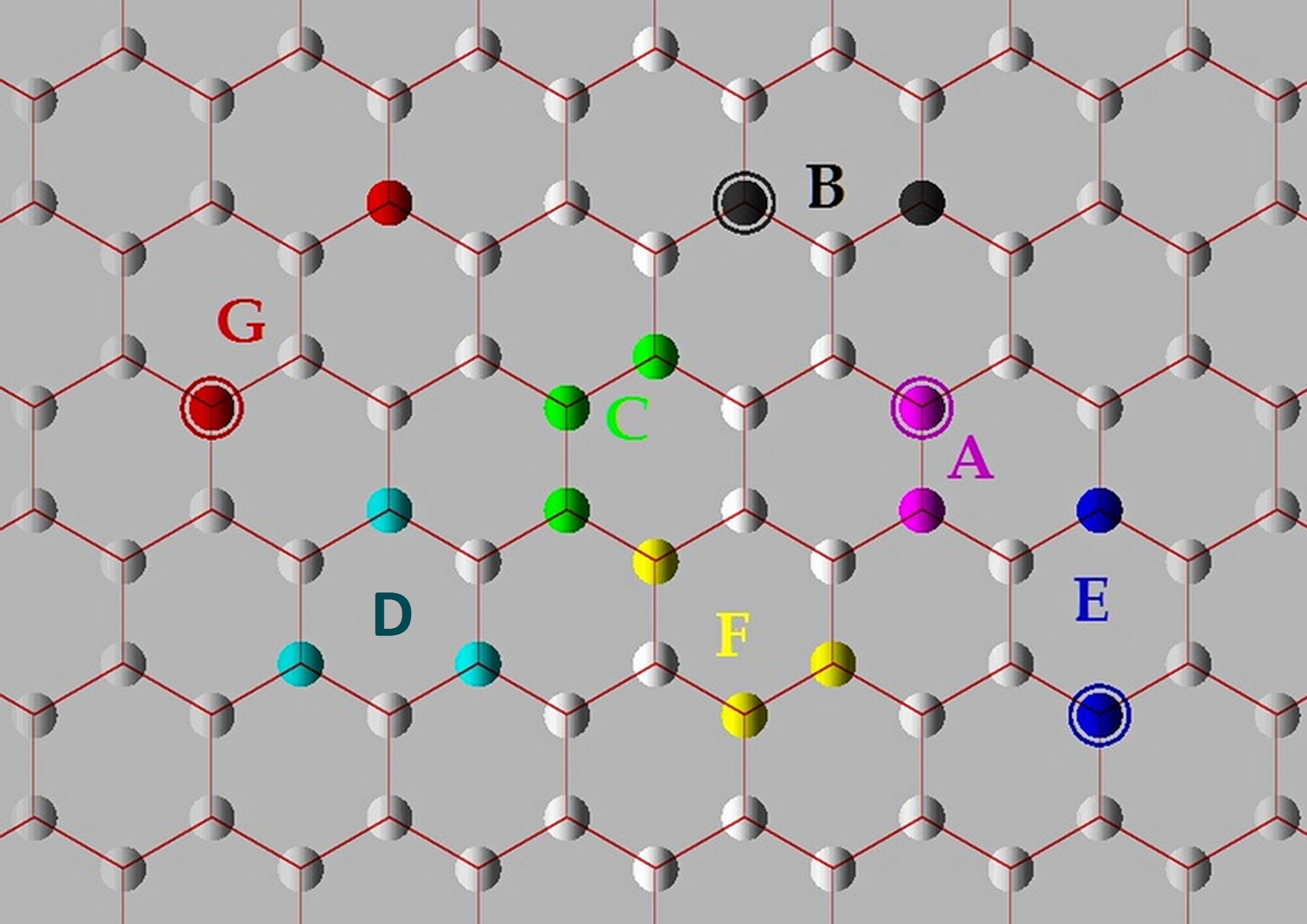
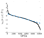
Figure 2: (Color online) Left) CFC types $A$ to $G$ on a graphene sheet. $A,B$ and $G$ contains a singly occupied site and a doubly occupied site, while $C,D,E,F$ have all of their three sites singly occupied. Types $E$ and $F$ involve third nearest neighbors, while type $G$ involve a fourth nearest neighbor. Only one copy of each type is shown here; the rest are related by rotation, reflection or translation symmetry. Right) Logplot of magnitudes of all the CFC coefficients in graphene, according to data from Ref. Lindsay et al., 2014. Beyond the several dominant types of terms, the remaining IFCs are much smaller and distributed exponentially (dashed blue guiding line).

We consider seven types of CFCs $A,B,...,G$ involving at most fourth nearest neighbors on the honeycomb lattice, as shown in Fig 2. By carefully keeping track of the all the terms related by symmetry, as well as their relative signs, the uniaxial (anisotropic) Grüneisen parameter can be expressed (via Eq. 22) in the form

$$\gamma_{{\bm{q}}s}(F)=\frac{1}{2M\omega_{{\bm{q}}s}^{2}}\sum_{jj^{\prime}}[\epsilon^{j}_{{\bm{q}}s}]^{*}\Gamma^{jj^{\prime}}(F)\epsilon_{{\bm{q}}s}^{j^{\prime}}$$ (23)

where $\Gamma(F)=\Gamma_{A}+\Gamma_{B}...+\Gamma_{G}$ is a sum of $2\times 2$ matrices $\Gamma_{A},...,\Gamma_{G}$ containing the contributions from the seven types of CFCs. The explicit forms of these matrices are presented in Appendix D. From Eq. 22, we obtain a few simplifying relations $\Gamma^{11}=(\Gamma^{22})^{*}$ and $\Gamma^{12}=(\Gamma^{21})^{*}$. Hence $\Gamma$ can also be decomposed in terms of the Pauli matrices via $\Gamma=\tau_{0}\,\mathit{I}+{\bm{\tau}}\cdot{\bm{\sigma}}$ where ${\bm{\tau}}=(\tau_{1},\tau_{2},i\tau_{3})$. The uniaxial Grüneisen parameter simplifies to

$$\gamma_{{\bm{q}}\pm}(F) = \frac{1}{2M\omega_{{\bm{q}}\pm}^{2}}[\epsilon_{{\bm{q}}\pm}]^{*}\cdot\Gamma\cdot\epsilon_{{\bm{q}}\pm}$$ (24)

$$= \frac{1}{2M\omega_{{\bm{q}}\pm}^{2}}[\epsilon_{{\bm{q}}\pm}]^{*}\cdot(\tau_{0}\mathit{I}+{\bm{\tau}}\cdot{\bm{\sigma}})\cdot\epsilon_{{\bm{q}}\pm}$$

$$= \frac{1}{2M\omega_{{\bm{q}}\pm}^{2}}\left(\tau_{0}({\bm{q}})\pm{\bm{\tau}}({\bm{q}})\cdot\hat{{\bm{d}}}({\bm{q}})\right)$$

where $\hat{{\bm{d}}}=\frac{1}{\sqrt{d_{1}^{2}+d_{2}^{2}}}(d_{1},d_{2})$, $d_{1}$ and $d_{2}$ being explicitly given in Eqs. 38 and 39 for the tight-binding model given above. In our subsequent numerical computations, we shall however directly use polarization vector data from DFT. Note that $d_{0}$ cannot affect the polarization vectors, and do not enter Eq. 24 at all. Equation 24 elegantly expresses the Grüneisen parameter in terms of the “vectors” $\hat{{\bm{d}}}$ and ${\bm{\tau}}$ characterizing the quadratic and cubic IFCs, respectively, and is in fact applicable to a generic 2-band phonon model. Recalling that the physical interpretation of $\gamma_{{\bm{q}}s}(F)$ as the fractional change in $\omega_{{\bm{q}}s}$ due to a fractional deformation in the direction of $\hat{{\bm{f}}}$, we see that the change of $\omega^{2}_{{\bm{q}}s}$ depends not just on the magnitude of the CFCs per se (as in a monoatomic lattice, see Appendix D), but also on their relative alignment with the quadratic IFCs in sublattice space. Specifically,

1. The contribution $\tau_{0}=\frac{\Gamma_{11}+\Gamma_{22}}{2}$ exists independently from the phonon dispersion. It has equal weight in both sublattices, and couples to the (constant) normalization of $\epsilon_{\pm}$.

2. The contribution ${\bm{\tau}}\cdot\hat{{\bm{d}}}$ depends on the phonon dispersion via $\hat{{\bm{d}}}({\bm{q}})$. It arises from the couplings between the inter-sublattice components of $\Phi$ and $\Psi(\hat{{\bm{r}}}\cdot\hat{{\bm{f}}})^{2}$, which represent the quadratic and cubic IFCs, respectively.

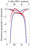
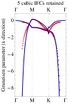
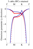
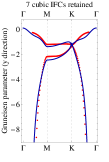
Figure 3: (Color online) Comparison between the anisotropic Grüneisen parameters $\gamma_{{\bm{q}}s}(\hat{x}),\gamma_{{\bm{q}}s}(\hat{y})$ obtained directly via DFT (red dotted curve), with those calculated from reverse-engineered CFCs via Eq. 24 (blue continuous curves), as described in the main text. Their agreement increases significantly as more CFCs are retained: The left,center and right columns depict cases with $\{A,B,C\}$ types, $\{A,B,C,D,E\}$ types, and all seven CFC types $A$ to $G$, respectively.

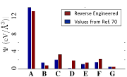
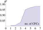
Figure 4: (Color online) (Left) The relative magnitudes of the CFCs of types $A$ to $G$ we reversed engineered from our DFT data. The NN type $A$ dominates, but the NNN type $B$ has almost zero weight. Of also little importance is the NNNNN type $G$. Note the good agreement with established data from Ref. Lindsay et al., 2014, at least for the more dominant CFCs. (Right) The agreement of fit of Fig 3, i.e. the comparison of the Gruneisen parameters directly obtained from DFT, versus those computed from the reverse engineered CFCs via Eq. 17. This agreement, which is quantified by the $R^{2}$ score, is plotted for different numbers of nonzero CFCs types $A$ through $G$. It improves significantly after adding the $D$-type CFC to types $A$ to $C$.

In Fig. 3, we demonstrate the fidelity of the reverse-engineering of the CFCs from DFT data, as described in Sect. III. The uniaxial Grüneisen parameters $\gamma_{{\bm{q}}\pm}(\hat{x})$ and $\gamma_{{\bm{q}}\pm}(\hat{y})$ are first computed via DFT (red dotted curves). We note that under an uniaxial deformation, the crystal type changes from hexagonal to orthorhombic base-centered and the total CPU time for one set of phonon calculations (for a complete phonon dispersion with 73 irreducible $k$ points) is typically less than 50 cpu hours on a Intel(R) Xeon(R) $2.30$ GHz multi-CPU workstation. By substituting the polarization vectors in Eq. 13 with the polarization eigenvectors obtained from DFT ,the Grüneisen parameters was used to obtain the coefficients of seven shortest range nonzero CFCs of the forms $A,B,...,G$, as described in Fig. 2 and numerically presented in fig. 4. In this simple example of flexural graphene, Eq. 13 reduces to Eq. 24 had tight-binding parameters been used for the harmonic part of the phonon potential.

The truncation of the CFCs leads to an incomplete basis, and we cannot expect to obtain perfectly accurate reverse-engineered CFC coefficients. To investigate how closely they resemble the true CFC coefficients, we compare their corresponding uniaxial Grüneisen parameter curves with those obtained from DFT in Figs. 3 and 4. We observe rather good agreement (with goodness-of-fit parameter $R^{2}>0.95$) upon the inclusion of $4$ or more CFCs, and even better agreement ($R^{2}>0.98$) with all seven types of CFCs $A$ to $G$. Explicitly, the individual CFCs reversed engineered from our DFT data also exhibit rather good agreement with established resultsLindsay et al. (2014), especially for types A,B,C,E and G.

This overall reasonable agreement suggests the usefulness of our reverse-engineering approach: with the Grüneisen parameters obtained from just a few DFT computations (one for each direction), we can already generate the largest CFCs rather accurately. This is contrasted with conventional, more computationally expensive DFPT methods that obtain the full set of CFCs through individual lattice perturbations. Note the crucial role of the directionality of the anisotropic Grüneisen parameters in isolating the CFCs: had the reverse engineering been performed with the (usual) isotropic Grüneisen parameter instead, only a certain linear combination of the CFCs could have been extracted, as elaborated at the end of Appendix D.

IV.4 Thermal conductivity of flexural modes

Finally, we shall illustrate the physical correctness of our CFC results by using them to calculate the thermal conductivity contribution from the acoustic flexural mode of graphene. This mode provides the largest contribution to the conductivity of graphene at room temperature or belowPaulatto et al. (2013), and can indeed be estimated fairly accurately by our approach.

The peculiar quadratic dispersion of the acoustic flexural mode $Z_{A}$ places selection rules on possible three phonon scattering processes from the $Z_{A}$ channelBonini et al. (2007). Specifically, only processes involving two $Z_{A}$ phonons and one transverse or longitudinal in-plane ($P_{A}$) acoustic phonon are permittedLindsay et al. (2010). As such, the phonon broadening width (Eq. 10), which is integral to computing the conductivity, can be simplified to

$$\tau_{{\bm{q}},Z_{A}}^{-1} = \frac{\pi\hbar}{4N}\sum_{{\bm{q}}^{\prime}}|M_{{\bm{q}},Z_{A},{\bm{q}}^{\prime},Z_{A},-{\bm{q}}-{\bm{q^{\prime}}},P_{A}}|^{2}$$

$$\times(n_{{\bm{q}}^{\prime},Z_{A}}-n_{-{\bm{q}}-{\bm{q}}^{\prime},P_{A}})\delta_{\omega_{{\bm{q}}^{\prime},Z_{A}}+\omega_{{\bm{q}},Z_{A}}-\omega_{-{\bm{q}}-{\bm{q}}^{\prime},P_{A}}}.$$

To proceed, the matrix elements $M_{{\bm{q}},Z_{A},{\bm{q}}^{\prime},Z_{A},-{\bm{q}}-{\bm{q^{\prime}}},P_{A}}$ are evaluated in terms of our reverse-engineered CFCs via Eq. 11. The polarization vectors $\epsilon_{{\bm{q}},P_{A}}$ and $\epsilon_{{\bm{q}},Z_{A}}$ in Eq. 11 can be obtained by diagonalizing the stiffness matrix in Eq. 17.

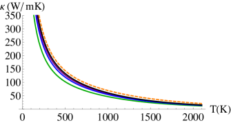
Figure 5: (Color online) The thermal conductivity due to the $Z_{A}$ flexural mode of graphene, plotted as a function of temperature. Plotted are the contributions from only the A-type CFC (Green), as well as contributions from the closest 5 (Blue), 6 (Purple) and 7 (Black) CFCs. We observe a convergence towards established results (orange dashed curve) computed with an extremely fine meshPaulatto et al. (2013), with the slight underestimate of less than $10\%$ attributable to the small number of CFCs we included. All CFCs were reverse-engineered from Grüneisen parameter data via Eq. 13, with polarization vectors obtained from DFT.

Notably, the thermal conductivity $\kappa$ diverges as $\sim T^{-1}$ at low temperatures. This can be understood from the small ${\bm{q}}$ behavior of $\tau_{{\bm{q}},Z_{A}}^{-1}$. Since the $P_{A}$ modes are linearly dispersive with much steeper slopes than that of $Z_{A}$ (see Fig. 1), we necessarily require ${\bm{q}}\approx-{\bm{q}}^{\prime}$ for simultaneous satisfaction of momentum and energy conservation. This leads to further simplification of Eq. LABEL:tau4 via $n_{{\bm{q}}^{\prime},Z_{A}}-n_{-{\bm{q}}-{\bm{q}}^{\prime},P_{A}}\approx(2\sinh x_{{\bm{q}},Z_{A}})^{-1}$, $x_{{\bm{q}},Z_{A}}=\frac{\hbar\omega_{{\bm{q}},Z_{A}}}{2k_{B}T}$. With that, one deduces that $\tau_{{\bm{q}},Z_{A}}^{-1}$ vanishes quadratically around the $\Gamma$ point, in agreement with results from Ref. Paulatto et al., 2013. Together with the approximate $(2\sinh x_{{\bm{q}},Z_{A}})^{-1}$ factor from the occupation functions, the $\kappa\sim T^{-1}$ behavior follows from simple Taylor expansion.

As demonstrated in Fig. 5 our results deviate from that of a much more exhaustive computation (Ref. Paulatto et al., 2013) by not more than $10\%$, a reasonable margin given that we have included contributions from only the seven types of CFC mentioned. Due to the smallness of the CFCs beyond the fifth, we observe a nice convergence pattern when more than 5 CFCs are included. Larger values of $\kappa$ from both ours and Ref. Paulatto et al., 2013’s results were reported by other works i.e. Ref. Lindsay et al., 2014. This discrepancy is most probably due to the relaxation-time approximation, which may not be very accurate for graphene. Secondarily, we have also excluded contributions from phonon-isotope and boundary scattering, both of which are beyond the scope of this study on anharmonicity.

V Discussion and Conclusion

We have proposed and demonstrated a general approach for determining the most important third-order interatomic force constants (also called the cubic force constants (CFCs)) from Grüneisen parameter data corresponding to deformations in appropriately chosen directions. This approach can be viewed as a hybrid between real and reciprocal space approaches, where a derivative corresponding to a real-space deformation is applied to the dynamical matrix defined in reciprocal space. The high efficiency of our approach critically hinges upon the optimal use of density-functional perturbation theory (DFPT) in phonon calculations, where a primitive cell is all that is required for deriving the phonon dispersions. To facilitate the retrieval of the CFCs, we have derived a most general expression for the Grüneisen parameters corresponding to very general deformation on all (seven) crystal types.

That our approach even works appears counterintuitive at first sight, since Grüneisen parameters are defined with respect to uniform crystal distortions while the CFCs obviously have to be probed with independent individual atomic displacements. Yet, by virtue of the locality of typical atomic orbitals, we showed that Grüneisen data can indeed be used to “reverse engineer” the values of a small but very important fraction of the CFCs. Testimony to the reliability of our approach is the excellent fit of our “reverse engineered” CFCs of graphene to well-established results on the Grüneisen parameter, which also results in reasonably accurate predictions of the conductivity due to the flexural channel. It is expected that with systematic computer implementation of the general approach outlined in this paper, anharmonic effects such as the thermal conductivity of technologically important materials can be efficiently and routinely predicted with a first-principles treatment.

VI Acknowledgments

We gratefully acknowledge the harmonic and anharmonic force constants provided by Lucas Lindsay of Oak Ridge National Laboratory.

Appendix A Derivation of thermal expansion in terms of Grüneisen parameters

Here we derive from first principles Eq. 7, which relates the thermal expansion coefficient (TEC) $\alpha$ in terms of the phonon mode heat capacities and Grüneisen parameters. $\alpha$ is defined as the fractional change in volume $V$ with temperature $T$ measured at pressure $P=0$:

$$\alpha=\left.\frac{1}{V}\frac{\partial V}{\partial T}\right|_{P=0}$$ (26)

To derive its explicit dependence on the Grüneisen parameters and hence the CFCs, we first note that the condition $P=0$, where $\alpha$ is defined, constraints the lattice free energy $F$ via

$$P=-\left.\frac{\partial F}{\partial V}\right|_{T}=-\left.\frac{\partial F_{\rm PE}}{\partial V}\right|_{T}-\left.\frac{\partial F_{\rm KE}}{\partial V}\right|_{T}=0$$ (27)

where $F_{\rm PE}$ and $F_{\rm KE}$ are the potential and kinetic portions of the free energy. The first term is related to $\Delta V$, the volume change due to increasing temperature via $\left.\frac{\partial F_{\rm PE}}{\partial V}\right|_{T}=C\Delta V$, which is proportional to the elastic constant matrix $C$. The second term $F_{\rm KE}=\hbar\sum_{{\bm{q}}s}\omega_{{\bm{q}}s}$ is a sum over the mode energies, so $\left.\frac{\partial F_{\rm KE}}{\partial V}\right|_{T}=\hbar\sum_{{\bm{q}}s}\frac{\partial F_{\rm KE}}{\omega_{{\bm{q}}s}}\frac{\partial\omega_{{\bm{q}}s}}{\partial V}=-\sum_{{\bm{q}}s}\frac{V\bar{\epsilon}_{{\bm{q}}s}}{\omega_{{\bm{q}}s}}\frac{\partial\omega_{{\bm{q}}s}}{\partial V}=\sum_{{\bm{q}}s}\gamma_{{\bm{q}}s}\bar{\epsilon}_{{\bm{q}}s}$ where $\bar{\epsilon}_{{\bm{q}}s}$ is the equilibrium energy of the phonon mode. Combining the above in Eqs. 26 and 27 and employing the tensorial properties of the derivatives, we obtain Eq. 7:

$$\alpha_{i}=\frac{1}{\Omega}C^{-1}_{ij}I_{j},$$ (28)

$$I_{j}=\frac{\Omega}{V}\sum_{{\bm{q}}s}\gamma_{{\bm{q}}s}c_{{\bm{q}}s},$$ (29)

where $c_{{\bm{q}}s}=\left.\frac{\partial\bar{\epsilon}_{{\bm{q}}s}}{\partial T}\right|_{V}$ is the phonon mode heat capacity, and $\Omega$ the equilibrium unit cell volume.

Appendix B Spring toy model

To provide a pedagogical and explicit illustration of how the CFCs contribute to the Grüneisen parameter, we consider a toy model of a rectangular lattice of anharmonic springs. Denote the length, stiffness and direction vector of each spring as $a$, $k$ and $\hat{{\bm{n}}}$. A spring between lattice sites $l$ and $l+1$ contributes a potential energy of

$$U_{l} = \frac{k}{2}(\hat{{\bm{n}}}\cdot\Delta{\bm{u}})^{2}+\frac{\lambda}{6}(\hat{{\bm{n}}}\cdot\Delta{\bm{u}})^{3}$$

$$= \frac{k}{2}\sum_{\alpha\beta}\Delta u^{\alpha}[\hat{{\bm{n}}}\hat{{\bm{n}}}^{T}]^{\alpha\beta}\Delta u^{\beta}+\frac{\lambda}{6}\sum_{\alpha\beta\gamma}\hat{{\bm{n}}}^{\alpha}\hat{{\bm{n}}}^{\beta}\hat{{\bm{n}}}^{\gamma}\Delta u^{\alpha}\Delta u^{\beta}\Delta u^{\gamma}$$

where $\Delta{\bm{u}}={\bm{u}}_{l+1}-{\bm{u}}_{l}$ is the difference between the displacements about the equilibrium positions at sites $l+1$ and $l$. These sites themselves are physically separated by a displacement $a\hat{{\bm{n}}}$. By expanding $(\Delta{\bm{u}})^{3}=({\bm{u}}_{l+1}-{\bm{u}}_{l})^{3}$ and summing over the lattice, the cubic term in Eq. LABEL:Ui takes the form

$$\frac{1}{6}\sum_{\alpha\beta\gamma}\sum_{l,l^{\prime},l^{\prime\prime}}\Psi^{\alpha\beta\gamma}_{l,l^{\prime},l^{\prime\prime}}u_{l}^{\alpha}u_{l^{\prime}}^{\beta}u_{l^{\prime\prime}}^{\gamma}$$

$$= \frac{\lambda}{6}\sum_{\alpha\beta\gamma}\left[\hat{{\bm{n}}}^{\alpha}\hat{{\bm{n}}}^{\beta}\hat{{\bm{n}}}^{\gamma}\left(\sum_{l,l^{\prime},l^{\prime\prime}}\delta_{l^{\prime}l}(\delta_{l^{\prime\prime},l+1}-\delta_{l^{\prime\prime},l-1})+\delta_{l^{\prime},l+1}(\delta_{l^{\prime\prime},l}-\delta_{l^{\prime\prime},l+1})+\delta_{l^{\prime},l-1}(\delta_{l^{\prime\prime},l-1}-\delta_{l^{\prime\prime},l})\right)\right]u_{l}^{\alpha}u_{l^{\prime}}^{\beta}u_{l^{\prime\prime}}^{\gamma}$$

The quantity in the parentheses are just the six surviving cross terms, given for instance by $-u_{l}^{\alpha}u_{l}^{\beta}u_{l-1}^{\gamma}\hat{{\bm{n}}}^{\alpha}\hat{{\bm{n}}}^{\beta}\hat{{\bm{n}}}^{\gamma}$ or $u_{l}^{\alpha}u_{l-1}^{\beta}u_{l-1}^{\gamma}\hat{{\bm{n}}}^{\alpha}\hat{{\bm{n}}}^{\beta}\hat{{\bm{n}}}^{\gamma}$.

To compute the Grüneisen parameter, we substitute $a\hat{{\bm{n}}}=a(\cos\theta,\sin\theta)^{T}$ for $r^{\gamma}_{j^{\prime\prime}l^{\prime\prime}}$ in Eq. 5. For the case of a trivial unit cell, the $j$ sublattice index is irrelevant and the quantity in the square parentheses of Eq. 5 simplifies to

$$\sum_{l^{\prime}}e^{i{\bm{q}}\cdot{\bm{R}}_{l^{\prime}}}\left(\sum_{l^{\prime\prime},\gamma}\Psi^{\alpha\beta\gamma}_{0l^{\prime}l^{\prime\prime}}r_{l^{\prime\prime}}^{\gamma}\right)=2a\lambda(1-\cos[a{\bm{q}}\cdot\hat{{\bm{n}}}])\left[\hat{{\bm{n}}}\hat{{\bm{n}}}^{T}\right]^{\alpha\beta}$$ (32)

We next make use of $[\epsilon_{s}^{\alpha}]^{*}\left[\hat{{\bm{n}}}\hat{{\bm{n}}}^{T}\right]^{\alpha\beta}\epsilon_{s}^{\beta}=|{\bm{\epsilon}}_{s}^{*}\cdot\hat{{\bm{n}}}|^{2}$ to obtain, for a lattice with various spring types $i=1,2,...$,

$$\gamma_{{\bm{q}}s} = \frac{1}{\Lambda M\omega^{2}_{{\bm{q}},s}}\sum_{i}\lambda_{i}a_{i}(1-\cos[a_{i}{\bm{q}}\cdot\hat{{\bm{n}}}_{i}])|{\bm{\epsilon}}_{{\bm{q}}s}^{*}\cdot\hat{{\bm{n}}}_{i}|^{2}$$

where $M$ is the mass of each atom. In the simplest case of a 1-dimensional lattice with a trivial unit cell, ${\bm{\epsilon}}_{s}$ is trivial and $|{\bm{\epsilon}}_{{\bm{q}}s}^{*}\cdot\hat{{\bm{n}}}_{i}|^{2}=1$.

If the lattice is 2-dimensional, but still with a trivial unit cell, ${\bm{\epsilon}}_{s}$ has two polarization components and we can simplify Eq. LABEL:gammae via Eq. 24 to obtain

$$= \frac{1}{2\Lambda M\omega^{2}_{{\bm{q}},\pm}}\sum_{i}\lambda_{i}a_{i}(1-\cos[a_{i}{\bm{q}}\cdot\hat{{\bm{n}}}_{i}])(1\pm\cos(2\theta_{i}-\varphi({\bm{q}})))$$

where $d_{1}=d\sin\varphi$, $d_{3}=d\cos\varphi$. The last line can also be obtained via the explicit form of $\epsilon_{\pm}$ from Eq. 20.

For a simplest example, consider the case with only one type of spring (i.e., a linear mono-atomic chain), $d_{0}(q)=d(q)$, $d_{1}(q)=d(q)\sin 2\theta$, $d_{3}(q)=d(q)\cos 2\theta$, so that we simply have $\varphi=2\theta$. This yields $\gamma_{q,+}=\frac{\lambda a}{2kD}=\frac{\lambda a}{2k}$ for the optical mode, in agreement with textbook calculations.Mihaly and Martin (1996)

Appendix C Determination of the dynamical matrices for a monoatomic and a diatomic system

C.1 Monoatomic lattice with non-rigid springs

To find the dynamical matrix (Eq. 2), one takes the Fourier transform of the real space quadratic IFCs. In a monoatomic lattice, the sublattice index $j$ is irrelevant and we write $D({\bm{q}})=d_{0}\mathit{I}+{\bm{d}}\cdot{\bm{\sigma}}$, where ${\bm{\sigma}}$ is the vector of Pauli matrices. Each non-rigid spring in the direction $\hat{{\bm{n}}}$ can only exert a force of $-(\Delta{\bm{u}}\cdot\hat{{\bm{n}}})\hat{{\bm{n}}}\propto\hat{{\bm{n}}}$, where $\Delta{\bm{u}}$ is the difference of the displacements ${\bm{u}}$ of its two ends.

In a monoatomic lattice, each atom is connected by equivalent springs in opposite directions, with extensions given by $\Delta{\bm{u}}={\bm{u}}_{l+1}-{\bm{u}}_{l}$ and $\Delta{\bm{u}}={\bm{u}}_{l}-{\bm{u}}_{l-1}$. Hence a pair of springs along the direction $\hat{{\bm{n}}}=(\cos\theta,\sin\theta)^{T}$ contributes a factor of

$$\frac{k}{M}(2-e^{ia{\bm{q}}\cdot\hat{{\bm{n}}}}-e^{-ia{\bm{q}}\cdot\hat{{\bm{n}}}})(\hat{{\bm{n}}}\hat{{\bm{n}}}^{T})$$

$$= \frac{k}{M}(1-\cos[a{\bm{q}}\cdot\hat{{\bm{n}}}])(\mathit{I}+\sigma_{1}\sin 2\theta+\sigma_{3}\cos 2\theta)$$

to $D({\bm{q}})$, where $M$ is the mass of each atom, $a$ the spring length and $k$ the spring stiffness. If each atom is attached to springs of stiffness $k_{1},k_{2},...$, lengths $a_{1},a_{2},...$ oriented in directions $\hat{{\bm{n}}}_{i}=(\cos\theta_{i},\sin\theta_{i})^{T}$, $i=1,2,...$, we have

$$d_{0}=\frac{1}{M}\sum_{i}k_{i}(1-\cos[a_{i}{\bm{q}}\cdot\hat{{\bm{n}}}_{i}])$$ (36a)

$$d_{1}=\frac{1}{M}\sum_{i}k_{i}(1-\cos[a_{i}{\bm{q}}\cdot\hat{{\bm{n}}}_{i}])\sin 2\theta_{i}$$ (36b)

$$d_{3}=\frac{1}{M}\sum_{i}k_{i}(1-\cos[a_{i}{\bm{q}}\cdot\hat{{\bm{n}}}_{i}])\cos 2\theta_{i}$$ (36c)

$$d_{2}=0$$ (36d)

Note that with ${\bm{d}}$ living in the space of phonon polarizations, as above (but not in the following subsection), we always have $d_{2}=0$ in the presence of time-reversal symmetry.

C.2 Flexural modes on diatomic graphene lattice

In the case of flexural (out-of-plane) phonon modes in the force constant model of graphene (Eq. 17), we also have a decoupled two-band sector due to the decoupling of in-plane and out-of-plane modes. However, these two bands now represent sublattice DOFs associated with out-of-plane movements of atoms, rather than the $x$ and $y$ polarizations studied in Section—C.1. By taking lattice Fourier transforms (see Fig. 2), we find $D({\bm{q}})=\frac{1}{M}{\bm{\sigma}}\cdot{\bm{d}}({\bm{q}})$ with ${\bm{q}}=\frac{1}{a}(q_{1},q_{2})$, $a$ being the lattice constant, and

$$d_{0} = 3t_{1}+2t_{2}(3-\cos q_{1}-\cos q_{2}-$$ (37)

$$\cos(q_{1}+q_{2}))+3t_{3}+6t_{4}$$

$$d_{1} = t_{1}(1+\cos q_{1}+\cos(q_{1}+q_{2}))+$$ (38)

$$t_{3}(2\cos q_{2}+\cos(2q_{1}+q_{2}))+$$

$$t_{4}(\cos q_{1}+\cos 2q_{1}+2\cos q_{1}\cos q_{2}+$$

$$\cos(q_{1}+2q_{2})+\cos(2q_{1}+2q_{2}))$$

$$d_{2} = t_{1}(\sin q_{1}+\sin(q_{1}+q_{2}))+t_{3}(\sin(2q_{1}+q_{2}))+$$ (39)

$$t_{4}(-\sin q_{1}+\sin 2q_{1}+\sin(q_{1}-q_{2})+\sin(q_{1}+q_{2})+$$

$$\sin(q_{1}+2q_{2})+\sin(2q_{1}+2q_{2}))$$

$$d_{3} = 0$$ (40)

where $t_{1},t_{2},t_{3},t_{4}$ are the first, second, third and fourth nearest-neighbor quadratic IFC coefficients given by Ref. Zimmermann et al., 2008. Note that we now have $d_{3}=0$ due to sublattice symmetry, in contrast to the spring systems treated in section C.1, where $d_{2}=0$.

Appendix D Grüneisen parameters from graphene CFCs

Here, we present the detailed expressions for $\Gamma$ in the expression for $\gamma_{{\bm{q}}s}(F)$ (Eqs. 23 and 24). These results are based on the CFCs $A$ to $G$ in Fig. 2, whose exact configurations affect $\Gamma$ via Eq. 17.

As explained in the main text, we always have $\Gamma^{11}=(\Gamma^{22})^{*}$ and $\Gamma^{12}=(\Gamma^{21})^{*}$. Denoting ${\bm{f}}=(\cos\theta_{f},\sin\theta_{f},0)$, we have

$$\Gamma_{A}^{12} =-\Psi_{A}\left(\cos^{2}\left(\frac{\pi}{2}-\theta_{f}\right)e^{-i(q_{1}+q_{2})}+\cos^{2}\left(\frac{\pi}{6}-\theta_{f}\right)+\cos^{2}\left(\frac{5\pi}{6}-\theta_{f}\right)e^{-iq_{1}}\right)$$ (41)

$$\Gamma_{A}^{11} =\frac{3}{2}\Psi_{A}$$ (42)

$$\Gamma_{B}^{12} =0$$ (43)

$$\Gamma_{B}^{11} =\Psi_{B}\left(\frac{3}{2}-\cos^{2}\left(\theta_{f}\right)e^{iq_{1}}-\cos^{2}\left(\frac{\pi}{3}-\theta_{f}\right)e^{i(q_{1}+q_{2})}-\cos^{2}\left(\frac{2\pi}{3}-\theta_{f}\right)e^{iq_{2}}\right)$$ (44)

$$\Gamma_{C}^{12} =\Psi_{C}\left(\cos^{2}\left(\frac{\pi}{2}-\theta_{f}\right)(e^{-iq_{1}}-1)+\cos^{2}\left(\frac{\pi}{6}-\theta_{f}\right)(e^{-i(q_{1}+q_{2})}-e^{-iq_{1}})+\cos^{2}\left(\frac{5\pi}{6}-\theta_{f}\right)(1-e^{-i(q_{1}+q_{2})})\right)$$ (45)

$$\Gamma_{C}^{11} =\Psi_{C}\left(\cos^{2}\left(\frac{\pi}{2}-\theta_{f}\right)(e^{-iq_{2}}-e^{-i(q_{1}+q_{2})})+\cos^{2}\left(\frac{\pi}{6}-\theta_{f}\right)(e^{i(q_{1}+q_{2})}-e^{iq_{1}})+\cos^{2}\left(\frac{5\pi}{6}-\theta_{f}\right)(e^{-iq_{1}}-e^{iq_{2}})\right)$$ (46)

$$\Gamma_{D}^{12} =0$$ (47)

$$\Gamma_{D}^{11} =2\Psi_{D}\left(\cos^{2}\left(\theta_{f}\right)(\cos q_{2}-\cos(q_{1}+q_{2}))+\cos^{2}\left(\frac{\pi}{3}-\theta_{f}\right)(\cos q_{1}-\cos q_{2})+\cos^{2}\left(\frac{2\pi}{3}-\theta_{f}\right)(\cos(q_{1}+q_{2})-\cos q_{1})\right)$$ (48)

$$\Gamma_{E}^{12} =-\Psi_{E}\left(\cos^{2}\left(\frac{\pi}{2}-\theta_{f}\right)e^{iq_{2}}+\cos^{2}\left(\frac{\pi}{6}-\theta_{f}\right)e^{-i(2q_{1}+q_{2})}+\cos^{2}\left(\frac{5\pi}{6}-\theta_{f}\right)e^{-iq_{2}}\right)$$ (49)

$$\Gamma_{E}^{11} =\frac{3}{2}\Psi_{E}$$ (50)

$$\Gamma_{F}^{12} =\Psi_{F}\left(\cos^{2}\left(\frac{\pi}{2}-\theta_{f}\right)(e^{-i(2q_{1}+q_{2})}-e^{-iq_{2}})+\cos^{2}\left(\frac{\pi}{6}-\theta_{f}\right)(e^{-iq_{2}}-e^{iq_{2}})+\cos^{2}\left(\frac{5\pi}{6}-\theta_{f}\right)(e^{iq_{2}}-e^{-i(2q_{1}+q_{2})})\right)$$ (51)

$$\Gamma_{F}^{11} =\Psi_{F}\left(\cos^{2}\left(\frac{\pi}{2}-\theta_{f}\right)(e^{iq_{1}}-e^{-iq_{1}})+\cos^{2}\left(\frac{\pi}{6}-\theta_{f}\right)(e^{iq_{2}}-e^{-iq_{2}})+\cos^{2}\left(\frac{5\pi}{6}-\theta_{f}\right)(e^{-i(q_{1}+q_{2})}-e^{i(q_{1}+q_{2})})\right)$$ (52)

$$\Gamma_{G}^{12} =-\Psi_{G}\left(\cos^{2}\left(\frac{\pi}{2}-\varphi-\theta_{f}\right)e^{-i(2q_{1}+2q_{2})}+\cos^{2}\left(\frac{\pi}{2}+\varphi-\theta_{f}\right)e^{-i(q_{1}+2q_{2})}+\cos^{2}\left(\frac{\pi}{6}-\varphi-\theta_{f}\right)e^{iq_{1}}\right)$$

$$\;\;\;\;-\Psi_{G}\left(\cos^{2}\left(\frac{\pi}{6}+\varphi-\theta_{f}\right)e^{i(q_{1}+q_{2})}+\cos^{2}\left(\frac{5\pi}{6}-\varphi-\theta_{f}\right)e^{i(q_{2}-q_{1})}+\cos^{2}\left(\frac{5\pi}{6}+\varphi-\theta_{f}\right)e^{-2iq_{1}}\right)$$ (53)

$$\Gamma_{G}^{11} =3\Psi_{G}$$ (54)

where $\varphi=\tan^{-1}\frac{\sqrt{3}}{5}$ arises from the the orientation of the fourth nearest-neighbor terms $\Gamma_{G}$. After simplification, $\Gamma=\tau_{0}\mathit{I}+{\bm{\tau}}\cdot\sigma$, where

$$\tau_{1} = \cos^{2}\left(\frac{\pi}{2}-\theta_{f}\right)\left(\Psi_{C}(\cos q_{1}-1)-\Psi_{A}\cos(q_{1}+q_{2})-\Psi_{E}\cos q_{2}+\Psi_{F}(\cos(2q_{1}+q_{2})-\cos q_{2})\right)$$

$$+\cos^{2}\left(\frac{\pi}{6}-\theta_{f}\right)\left(\Psi_{C}(\cos(q_{1}+q_{2})-\cos q_{1})-\Psi_{A}-\Psi_{E}\cos(2q_{1}+q_{2})\right)$$

$$+\cos^{2}\left(\frac{5\pi}{6}-\theta_{f}\right)\left(\Psi_{C}(1-\cos(q_{1}+q_{2}))-\Psi_{A}\cos q_{1}-\Psi_{E}\cos q_{2}+\Psi_{F}(\cos q_{2}-\cos(2q_{1}+q_{2}))\right)$$

$$-\Psi_{G}\left(\cos^{2}\left(\frac{\pi}{2}-\varphi-\theta_{f}\right)\cos(2q_{1}+2q_{2})+\cos^{2}\left(\frac{\pi}{2}+\varphi-\theta_{f}\right)\cos(q_{1}+2q_{2})+\cos^{2}\left(\frac{\pi}{6}-\varphi-\theta_{f}\right)\cos q_{1}\right)$$

$$-\Psi_{G}\left(\cos^{2}\left(\frac{\pi}{6}+\varphi-\theta_{f}\right)\cos(q_{1}+q_{2})+\cos^{2}\left(\frac{5\pi}{6}-\varphi-\theta_{f}\right)\cos(q_{2}-q_{1})+\cos^{2}\left(\frac{5\pi}{6}+\varphi-\theta_{f}\right)\cos 2q_{1}\right)$$

$$\tau_{2} = \cos^{2}\left(\frac{\pi}{2}-\theta_{f}\right)\left(\Psi_{C}\sin q_{1}-\Psi_{A}\sin(q_{1}+q_{2})+\Psi_{E}\sin q_{2}+\Psi_{F}(\sin q_{2}-\sin(2q_{1}+q_{2}))\right)$$

$$+\cos^{2}\left(\frac{\pi}{6}-\theta_{f}\right)\left(\Psi_{C}(\sin(q_{1}+q_{2})-\sin q_{1})-\Psi_{E}\sin(2q_{1}+q_{2})+2\Psi_{F}\sin q_{2}\right)$$

$$+\cos^{2}\left(\frac{5\pi}{6}-\theta_{f}\right)\left(-\Psi_{C}\sin(q_{1}+q_{2})-\Psi_{A}\sin q_{1}-\Psi_{E}\sin q_{2}-\Psi_{F}(\sin q_{2}-\sin(2q_{1}+q_{2}))\right)$$

$$+\Psi_{G}\left(-\cos^{2}\left(\frac{\pi}{2}-\varphi-\theta_{f}\right)\sin(2q_{1}+2q_{2})-\cos^{2}\left(\frac{\pi}{2}+\varphi-\theta_{f}\right)\sin(q_{1}+2q_{2})+\cos^{2}\left(\frac{\pi}{6}-\varphi-\theta_{f}\right)\sin q_{1}\right)$$

$$+\Psi_{G}\left(\cos^{2}\left(\frac{\pi}{6}+\varphi-\theta_{f}\right)\sin(q_{1}+q_{2})+\cos^{2}\left(\frac{5\pi}{6}-\varphi-\theta_{f}\right)\sin(q_{2}-q_{1})-\cos^{2}\left(\frac{5\pi}{6}+\varphi-\theta_{f}\right)\sin 2q_{1}\right)$$

$$\tau_{0} = \frac{3}{2}\left(\Psi_{A}+\Psi_{B}+\Psi_{E}+2\Psi_{G}\right)$$ (57)

$$+\cos q_{1}\left(-\Psi_{B}\cos^{2}\left(\theta_{f}\right)+\frac{\sqrt{3}}{2}(2\Psi_{D}-\Psi_{C})\sin 2\theta_{f}\right)$$

$$+\cos q_{2}\left(-\Psi_{B}\cos^{2}\left(\frac{2\pi}{3}-\theta_{f}\right)+\frac{\sqrt{3}}{2}(2\Psi_{D}-\Psi_{C})\sin 2(\theta_{f}+\pi/3)\right)$$

$$+\cos(q_{1}+q_{2})\left(-\Psi_{B}\cos^{2}\left(\frac{\pi}{3}-\theta_{f}\right)+\frac{\sqrt{3}}{2}(2\Psi_{D}-\Psi_{C})\sin 2(\theta_{f}+2\pi/3)\right)$$

The Grüneisen parameters due to an isotropic biaxial strain in the $xy$ plane can be obtained by summing up the uniaxial Grüneisen parameters with ${\bm{f}}=(\cos\theta_{f},\sin\theta_{f},0)$ and ${\bm{f}}=(\cos(\theta_{f}+\pi/2),\sin(\theta_{f}+\pi/2),0)$. Due to the identity $\cos^{2}q+\sin^{2}q=1$ for any $q$, we replace all occurrences of cosine squared terms in $\tau_{1},\tau_{2}$ and $\tau_{0}$ by $1$ so that

$$\tau_{1}|_{\rm iso} = -\Psi_{A}(1+\cos(q_{1}+q_{2})+\cos q_{1})-\Psi_{E}(2\cos q_{2}+\cos(2q_{1}+q_{2}))$$

$$-\Psi_{G}\left(\cos(2q_{1}+2q_{2})+\cos(q_{1}+2q_{2})+\cos q_{1}+\cos(q_{1}+q_{2})+\cos(q_{2}-q_{1})+\cos 2q_{1}\right)$$

$$\tau_{2}|_{\rm iso} = -\Psi_{A}(\sin(q_{1}+q_{2})+\sin q_{1})-\Psi_{E}\sin(2q_{1}+q_{2})+2\Psi_{F}\sin q_{2}$$

$$+\Psi_{G}\left(-\sin(2q_{1}+2q_{2})-\sin(q_{1}+2q_{2})+\sin q_{1}+\sin(q_{1}+q_{2})+\sin(q_{2}-q_{1})-\sin 2q_{1}\right)$$

$$\tau_{0}|_{\rm iso} = \frac{3}{2}\left(\Psi_{A}+\Psi_{B}+\Psi_{E}+2\Psi_{G}\right)-\Psi_{B}(\cos q_{1}+\cos q_{2}+\cos(q_{1}+q_{2}))$$ (60)

It is evident that with an isotropic biaxial strain, only certain linear combinations of the CFCs can be isolated.

References

• Born and Huang (1956) M. Born and K. Huang, Dynamical Theory of Crystal Lattices (Oxford University Press, London, 1956).
• Maradudin et al. (1965) A. A. Maradudin, E. W. Montroll,  and G. H. Weiss, Theory of Lattice Dynamics in the Harmonic Approximation (Academic, New York, 1965).
• Horton and Maradudin (1974) G. K. Horton and A. A. Maradudin, Dynamical Properties of Solids: Crystalline Solids, Fundamentals (North-Holland, Amsterdam, 1974).
• Salerno and Carusotto (2014) G. Salerno and I. Carusotto, EPL (Europhysics Letters) 106, 24002 (2014).
• Nash et al. (2015) L. M. Nash, D. Kleckner, A. Read, V. Vitelli, A. M. Turner,  and W. T. Irvine, Proceedings of the National Academy of Sciences 112, 14495 (2015).
• Wang et al. (2015) P. Wang, L. Lu,  and K. Bertoldi, Phys. Rev. Lett. 115, 104302 (2015).
• Süsstrunk and Huber (2015) R. Süsstrunk and S. D. Huber, Science 349, 47 (2015).
• Yang et al. (2015) Z. Yang, F. Gao, X. Shi, X. Lin, Z. Gao, Y. Chong,  and B. Zhang, Phys. Rev. Lett. 114, 114301 (2015).
• Zhu et al. (2015) X.-F. Zhu, Y.-G. Peng, X.-Y. Yu, H. Jia, M. Bao, Y.-X. Shen,  and D.-G. Zhao, arXiv preprint arXiv:1508.06243  (2015).
• Fleury et al. (2015) R. Fleury, A. Khanikaev,  and A. Alu, arXiv preprint arXiv:1511.08427  (2015).
• Paulose et al. (2015) J. Paulose, A. S. Meeussen,  and V. Vitelli, Proceedings of the National Academy of Sciences 112, 7639 (2015).
• Ong and Lee (2016) Z.-Y. Ong and C. H. Lee, Phys. Rev. B 94, 134203 (2016).
• Huber (2016) S. D. Huber, Nature Physics 12, 621 (2016).
• Liu et al. (2016) Y. Liu, Y. Xu, S.-C. Zhang,  and W. Duan, arXiv preprint arXiv:1606.08013  (2016).
• Lu et al. (2016) J. Lu, C. Qiu, L. Ye, X. Fan, M. Ke, F. Zhang,  and Z. Liu, Nature Physics  (2016).
• Lee et al. (2017) C. H. Lee, G. Li, G. Jin, Y. Liu,  and X. Zhang, arXiv preprint arXiv:1701.03385  (2017).
• Leibfried and Ludwig (1961) G. Leibfried and W. Ludwig, Solid State Phys. 12, 275 (1961).
• Broido et al. (2005) D. A. Broido, A. Ward,  and N. Mingo, Phys. Rev. B 72, 014308 (2005).
• Snyder and Toberer (2008) G. J. Snyder and E. S. Toberer, Nature Mater. 7, 105 (2008).
• Ward et al. (2009) A. Ward, D. A. Broido, D. A. Stewart,  and G. Deinzer, Phys. Rev. B 80, 125203 (2009).
• Garg et al. (2011) J. Garg, N. Bonin, B. Kozinsky,  and N. Marzari, Phys. Rev. Lett. 106, 045901 (2011).
• Zebarjadi et al. (2012) M. Zebarjadi, K. Esfarjani, M. S. Dresselhaus, Z. F. Ren,  and G. Chen, Enery Environ. Sci 5, 5147 (2012).
• Broido et al. (2012) D. A. Broido, L. Lindsay,  and A. Ward, Phys. Rev. B 86, 115203 (2012).
• Wang et al. (2007) J.-S. Wang, N. Zeng, J. Wang,  and C. K. Gan, Phys. Rev. E 75, 061128 (2007).
• Frank et al. (1995) W. Frank, C. Elsässer,  and M. Fähnle, Phys. Rev. Lett. 74, 1791 (1995).
• Kresse et al. (1995) G. Kresse, J. Furthmüller,  and J. Hafner, Europhys. Lett. 32, 729 (1995).
• Ackland et al. (1997) G. J. Ackland, M. C. Warren,  and S. J. Clark, J. Phys.: Condens. Matter 9, 7861 (1997).
• Parlinski et al. (1997) K. Parlinski, Z. Q. Li,  and Y. Kawazoe, Phys. Rev. Lett. 78, 4063 (1997).
• Alfè (2009) D. Alfè, Comp. Phys. Comm. 180, 2622 (2009).
• Gan et al. (2006) C. K. Gan, Y. P. Feng,  and D. J. Srolovitz, Phys. Rev. B 73, 235214 (2006).
• Gan et al. (2010) C. K. Gan, X. F. Fan,  and J.-L. Kuo, Comput. Mater. Sci. 49, S29 (2010).
• Liu et al. (2014) Y. Liu, K. T. E. Chua, T. C. Sum,  and C. K. Gan, Phys. Chem. Chem. Phys. 16, 345 (2014).
• Togo and Tanaka (2015) A. Togo and I. Tanaka, Scr. Mater. 108, 1 (2015).
• Togo et al. (2015) A. Togo, L. Chaput,  and I. Tanaka, Phys. Rev. B 91, 094306 (2015).
• Baroni et al. (1987) S. Baroni, P. Giannozzi,  and A. Testa, Phys. Rev. Lett. 58, 1861 (1987).
• Baroni et al. (2001) S. Baroni, S. de Gironcoli, A. Dal Corso,  and P. Giannozzi, Rev. Mod. Phys. 73, 515 (2001).
• Esfarjani and Stokes (2008) K. Esfarjani and H. T. Stokes, Phys. Rev. B 77, 144112 (2008).
• Shiomi et al. (2011) J. Shiomi, K. Esfarjani,  and G. Chen, Phys. Rev. B 84, 104302 (2011).
• Debernardi et al. (1995) A. Debernardi, S. Baroni,  and E. Molinari, Phys. Rev. Lett. 75, 1819 (1995).
• Paulatto et al. (2013) L. Paulatto, F. Mauri,  and M. Lazzeri, Phys. Rev. B 87, 214303 (2013).
• Zhou et al. (2014) F. Zhou, W. Nielson, Y. Xia,  and V. Ozolins, Phys. Rev. Lett. 113, 185501 (2014).
• Hellman and Abrikosov (2013) O. Hellman and I. A. Abrikosov, Phys. Rev. B 88, 144301 (2013).
• Pavone et al. (1993) P. Pavone, K. Karch, O. Schütt, W. Windl, D. Strauch, P. Giannozzi,  and S. Baroni, Phys. Rev. B 48, 3156 (1993).
• Mounet and Marzari (2005) N. Mounet and N. Marzari, Phys. Rev. B 71, 205214 (2005).
• Gan et al. (2015) C. K. Gan, J. R. Soh,  and Y. Liu, Phys. Rev. B 92, 235202 (2015).
• Liu et al. (2017) G. Liu, H. M. Liu, J. Zhou,  and X. G. Wan, J. Appl. Phys. 121, 045104 (2017).
• Arnaud et al. (2016) B. Arnaud, S. Lebègue,  and G. Raffy, Phys. Rev. B 93, 94106 (2016).
• Ding and Xiao (2015) Y. Ding and B. Xiao, RSC Adv. 5, 18391 (2015).
• Gan and Liu (2016) C. K. Gan and Y. Y. F. Liu, Phys. Rev. B 94, 134303 (2016).
• Michel et al. (2015) K. H. Michel, S. Costamagna,  and F. M. Peeters, Phys. Rev. B 91, 134302 (2015).
• Tadano and Tsuneyuki (2015) T. Tadano and S. Tsuneyuki, Phys. Rev. B 92, 054301 (2015).
• Note (1) In fact, the assumption of exclusively quadratic force constants leads to the paradoxical situation of the phonon bands remaining unchanged under arbitrarily large lattice distortion.
• Nye (1985) J. F. Nye, Physical Properties of Crystals: Their Representations by Tensors and Matrices (Clarendon, Oxford, 1985).
• Schelling and Keblinski (2003) P. K. Schelling and P. Keblinski, Phys. Rev. B 68, 035425 (2003).
• Srivastava (1990) G. P. Srivastava, The Physics of Phonons (CRC Press, 1990).
• Lindsay et al. (2010) L. Lindsay, D. Broido,  and N. Mingo, Phys. Rev. B 82, 115427 (2010).
• Note (2) It is the combination \sum@\slimits@γΨαβγfiγ\sum@subscript\slimits@𝛾superscriptΨ𝛼𝛽𝛾superscriptsubscript𝑓𝑖𝛾\sum@\slimits@_{\gamma}\Psi^{\alpha\beta\gamma}f_{i}^{\gamma}, rather than the CFCs $\Psi^{\alpha\beta\gamma}$ themselves that enter the Grüneisen parameter.
• He and Vanderbilt (2001) L. He and D. Vanderbilt, Phys. Rev. Lett. 86, 5341 (2001).
• Lee et al. (2016) C. H. Lee, D. P. Arovas,  and R. Thomale, Phys. Rev. B 93, 155155 (2016).
• Bonini et al. (2007) N. Bonini, M. Lazzeri, N. Marzari,  and F. Mauri, Phys. Rev. Lett. 99, 176802 (2007).
• Balandin et al. (2008) A. A. Balandin, S. Ghosh, W. Bao, I. Calizo, D. Teweldebrhan, F. Miao,  and C. N. Lau, Nano Lett. 8, 902 (2008).
• Tan et al. (2011) Z. W. Tan, J. -S. Wang,  and C. K. Gan, Nano Lett. 11, 214 (2011).
• Kong et al. (2009) B. D. Kong, S. Paul, M. B. Nardelli,  and K. W. Kim, Phys. Rev. B 80, 033406 (2009).
• Saito et al. (1998) R. Saito, G. Dresselhaus, M. S. Dresselhaus, et al.Physical properties of carbon nanotubes (World Scientific, 1998).
• Zimmermann et al. (2008) J. Zimmermann, P. Pavone,  and G. Cuniberti, Phys. Rev. B 78, 045410 (2008).
• Giannozzi et al. (2009) P. Giannozzi, S. Baroni, N. Bonini, M. Calandra, R. Car, C. Cavazzoni, D. Ceresoli, G. L. Chiarotti, M. Cococcioni, I. Dabo, A. Dal Corso, S. de Gironcoli, S. Fabris, G. Fratesi, R. Gebauer, U. Gerstmann, C. Gougoussis, A. Kokalj, M. Lazzeri, L. Martin-Samos, N. Marzari, F. Mauri, R. Mazzarello, S. Paolini, A. Pasquarello, L. Paulatto, C. Sbraccia, S. Scandolo, G. Sclauzero, A. P. Seitsonen, A. Smogunov, P. Umari,  and R. M. Wentzcovitch, J. Phys.: Condens. Matter 21, 395502 (2009).
• Note (3) In terms of the tight-binding parameters, the lack of compressive contributions is equivalent to the out-of-plane spring constants satisfying the sum rule (written here for the honeycomb lattice) $t_{1}+6t_{2}+4t_{3}+14t_{4}+...=0$, where $t_{i}$ refers to $K^{\perp}_{\rm out}$ for the $i$th nearest neighbor.
• Note (4) There is no $\Psi^{zzz}$ component due to antisymmetry.
• Note (5) Mathematically, a real 1-dimensional real representation of the dihedral group plus translation can only be the trivial representation.
• Lindsay et al. (2014) L. Lindsay, W. Li, J. Carrete, N. Mingo, D. A. Broido,  and T. L. Reinecke, Phys. Rev. B 89, 155426 (2014).
• Note (6) This can be shown by exchanging the sublattice indices $j$ and $j^{\prime}$, and simultaneously switching the origin of the vector $\mathaccentV{hat}05E{{\bm{r}}}_{j^{\prime\prime}l^{\prime\prime}}$.
• Note (7) Note the factor of $i$ in the third component; in general, $\Gamma$ does not have to be Hermitian.
• Note (8) Note that the CFCs corresponding to $u_{l}^{3}$ and $u_{l-1}^{3}$ annihilate each other.
• Mihaly and Martin (1996) L. Mihaly and M. C. Martin, Solid State Physics: Problems and Solutions (John Wiley and Sons, Inc, New York, 1996).
• Note (9) This expression is manifestly symmetric under $\mathaccentV{hat}05E{{\bm{n}}}\rightarrow-\mathaccentV{hat}05E{{\bm{n}}}$, as it should be.