Synchronizing Quantum Harmonic Oscillators through Two-Level Systems

Abstract

Two oscillators coupled to a two-level system which in turn is coupled to an infinite number of oscillators (reservoir) are considered, bringing to light the occurrence of synchronization. A detailed analysis clarifies the physical mechanism that forces the system to oscillate at a single frequency with a predictable and tunable phase difference. Finally, the scheme is generalized to the case of $N$ oscillators and $M(<N)$ two-level systems.

I Introduction

Synchronization processes in earlier definitions, imply the alignment of the dynamics of two or more periodically evolving physical systems ref:Pikovski2003 . In classical mechanics such processes are effectively described by the Kuramoto model ref_AcebronRMP2005 . Detailed studies, from basic physical laws, of the occurrence of synchronization in classical systems have been reported, especially considering pendula and metronomes ref_MaiantiAJP2009 ; ref_PantaleoneAJP2002 . Synchronization phenomena turn out to be relevant in several contexts, from neurosciences to medicine ref_Strogatz ; ref_AngeliniPRE2004 , which has naturally brought to the extension of the definition of synchronization to the dynamical alignment of complex and even chaotic systems ref_Arenas ; ref:Padmanaban .

Since the occurrence of synchronization has acquired attention in the realm of nanotechnologies, attempts to extend the Kuramoto model to the quantum realm have been made ref_deMendozaPRE2014 . Beyond the Kuramoto model, studies of synchronization in quantum systems have been developed ref_ZambriniPRA2010 ; ref_ZambriniPRA2012 ; ref_ZambriniSciRep2013 ; ref_StrogatzPRL2004 .

Because of the lack of trajectories in quantum mechanics, giving a proper definition of quantum synchronization is not as easy as in classical mechanics. Mutual information and specific correlations have been used, not only as a signature of dynamical alignment of quantum systems, but also to evaluate the degree of synchronization ref_FazioPRL2013 ; ref_FazioPRA2015 ; ref_ArmourPRA2015 .

In the last years, the paradigm of quantum synchronization has been extended from the first natural archetypical quantum system, i.e. the harmonic oscillator, to the other fundamental class of quantum systems, i.e. two-level systems (TLS). A few uncoupled spins interacting with a common environment ref_Plastina2013 as well as ensembles of dipoles ref_Zhu2015 have been considered. More recently, collective behavior of many spins has been studied in order to establish a connection between synchronization processes and superradiance or subradiance ref_Bellomo2017 . A further extension present in the literature is the dynamical alignment of optomechanical systems ref_Li2016 ; ref_Li2017 ; ref_Vitali2017 .

Synchronization in hybrid systems, involving oscillators and TLSs has been considered in the context of trapped ions in Ref ref_ArmourPRA2015 , where two oscillators (the centers of mass of the ions) are considered as coupled to the corresponding electronic degrees of freedom (modelled as two-level systems) which are coupled to the electromagnetic field. Because of the indirect interaction, the two oscillators eventually synchronize. It is worth mentioning that the expression ‘synchronization in hybrid systems’  has not to be confused with the ‘hybrid synchronization’  present in the literature which refers either to systems partially synchronized or to different systems which align, in spite of their different nature ref:Padmanaban ; ref_Qiu2015 . Moreover, the possibility to drive dynamical alignment of oscillators (a driven resonator) and TLSs (superconducting devices) has been predicted and demonstrated ref:Bistability2008 ; ref:ArtificialAtom2007 ; ref:Bistability2017 . In particular, it has been shown that the dynamical alignment bring to a significant change of the qubit radiation spectrum ref:Bistability2008 ; ref:ArtificialAtom2007

In this paper we will analyze a very simple hybrid model consisting of two oscillators coupled to a single two-level system, which in turn is coupled to an infinite number of oscillators (reservoir), in order to study in depth the mechanism of synchronization. We will show that the specific structure of the couplings between the oscillators and the TLS determines the structure of a preserved mode which in the long-time dynamics is responsible for a collective motion characterized by a single frequency. More detailed predictions about the phase difference between the oscillations can be made, on the basis of knowledge of the initial condition and of specific phase relations between the coupling constants of the oscillators with the TLS. Also the amplitudes of the position oscillations are easily predictable. The essential features of this model could be extended to its natural generalization, i.e. to the case of more than two oscillators and many two-level systems.

It is worth emphasizing that the relevance of our model is twofold. On the one hand, it shows that two ‘big’  systems (two oscillators, whose Hilbert spaces are infinite dimensional) can be synchronized by the action of a single ‘small’  one (a TLS), also providing an example of how two similar systems can be synchronized by a third part which has a completely different nature. This very point, a small (finite-level) system, which does not synchronize with the rest but which, at the same time, is responsible for making all the rest (a bigger, infinite-level system) synchronize, is a remarkable result. Of course, the key ingredient is that the TLS is interacting with the environment. On the other hand, the simplicity of the model (quantized oscillators and TLSs with dipole-like interactions) makes it relevant in many physical scenarios, from bimodal cavities to trapped ions to superconducting devices interacting with quantized fields. Moreover, such simplicity allows us to understand in a very clear way the mechanism of synchronization, as well as to predict the final common frequency of the oscillations, their amplitudes and possible phase differences.

The paper is structured as follows. In Sec.II we introduce the model and single out, qualitatively, some important dynamical features, while in Sec.III we show that in the long-time dynamics, for every initial state of the system, the two oscillators evolve with the same frequency. In Sec.V we generalize the model to the case of $N$ oscillators and $M(<N)$ TLSs. Finally, in Sec.VI we provide conclusive remarks.

II The Model

Consider a system governed by the following Hamiltonian:

$$H_{\mathrm{S}} = \sum_{k=1}^{2}\omega_{k}a^{\dagger}_{k}a_{k}+\frac{\omega_{0}}{2}\sigma_{z}+\sum_{k=1}^{2}g_{k}(\mathrm{e}^{\mathrm{i}\theta_{k}}a_{k}+\mathrm{e}^{-\mathrm{i}\theta_{k}}a_{k}^{\dagger})\sigma_{x}\,,$$

and assume that the two-level system (TLS) is coupled to an environment, here modelled as an infinite set of harmonic oscillators, each one linearly coupled to the two-level system:

$$H_{\mathrm{B}} = \sum_{i}\nu_{i}b_{i}^{\dagger}b_{i}\,,$$ (1b)

$$H_{\mathrm{I}} = \sum_{i}(\beta_{i}b_{i}+H.c.)\sigma_{x}\,.$$ (1c)

We will see in the following that this interaction with the environment is crucial, since, in addition with the interaction between the TLS and the oscillators, is responsible for the appearance of dissipating modes and stable modes.

II.1 ‘Single Leaking Mode Picture’  and Preserved Mode

Let us make a change of picture through the following unitary operators: a phase changing unitary operator,

$$U_{p}=\exp\left(\mathrm{i}\theta_{1}a_{1}^{\dagger}a_{1}+\mathrm{i}\theta_{2}a_{2}^{\dagger}a_{2}\right)\,,$$ (2a)

which transforms $$a_{k} \mathrm{e}^{-\mathrm{i}\theta_{k}}a_{k}$$ into , and a rotation unitary operator,

$$U_{r}=\exp\left[\gamma(a_{1}a_{2}^{\dagger}-a_{1}^{\dagger}a_{2})\right]\,,$$ (2b)

which realizes the following transformation:

$$a_{1} \rightarrow U_{r}a_{1}U_{r}^{\dagger}=\cos\gamma\,a_{1}+\sin\gamma\,a_{2}\,,$$ (2c)

$$a_{2} \rightarrow U_{r}a_{2}U_{r}^{\dagger}=-\sin\gamma\,a_{1}+\cos\gamma\,a_{2}\,,$$ (2d)

$$\sigma_{\alpha} \rightarrow U_{r}\sigma_{\alpha}U_{r}^{\dagger}=\sigma_{\alpha}\,,\qquad\alpha=x,y,z,\pm\,.$$ (2e)

The parameter $\gamma$ determines how the two modes are mixed, in this new picture (the Pauli operators are left unchanged for any $\gamma$).

The system Hamiltonian transformed by $U_{r}U_{p}$ (but expressed in terms of the original operators, $a_{k}$’s and $\sigma_{\alpha}$’s) is given by:

$$\tilde{H}_{\mathrm{S}} = \sum_{k=1}^{2}\tilde{\omega}_{k}a^{\dagger}_{k}a_{k}+\frac{\omega_{0}}{2}\sigma_{z}+\sum_{k=1}^{2}\tilde{g}_{k}(a_{k}+a_{k}^{\dagger})\sigma_{x}$$ (3a)

$$+ \left(\xi_{12}\,a_{1}^{\dagger}a_{2}+H.c.\,\right)\,,$$

with

$$\tilde{\omega}_{1} = \omega_{1}\cos^{2}\gamma+\omega_{2}\sin^{2}\gamma\,,$$ (3b)

$$\tilde{\omega}_{2} = \omega_{1}\sin^{2}\gamma+\omega_{2}\cos^{2}\gamma\,,$$ (3c)

$$\tilde{g}_{1} = g_{1}\cos\gamma-g_{2}\sin\gamma\,,$$ (3d)

$$\tilde{g}_{2} = g_{1}\sin\gamma+g_{2}\cos\gamma\,,$$ (3e)

$$\xi_{12} = (\omega_{1}-\omega_{2})\sin\gamma\,\cos\gamma\,.$$ (3f)

In this new picture, both the free energies of the oscillators and the coupling strengths of the oscillators with the TLS are modified. Moreover, because of the mixed algebra of the bosonic ($a_{k}$’s) and fermionic ($\sigma_{\alpha}$’s) operators, it is not possible to perfectly decouple the two modes, which implies that a tunnelling term between the two oscillators appears, the relevant strength being given by the parameter $\xi_{12}$.

By a suitable choice of the parameter $\gamma$,

$$\tan\gamma=\frac{g_{1}}{g_{2}}\,,$$ (4)

we obtain $\tilde{g}_{1}=0$ (and, by the way, $\tilde{g}_{2}=\sqrt{g_{1}^{2}+g_{2}^{2}}\,$), which implies that in this picture only one mode is directly coupled to the leaking TLS. (For this reason we will call this picture the ‘single leaking mode picture’ , or SLMP.) However, because of the coupling between the two modes ($\xi_{12}\not=0$), the other mode has an indirect coupling to the leaking TLS.

By imposing $\xi_{12}\ll\tilde{g}_{2}$ and $\xi_{12}$ much smaller than the decay rate of the TLS, we obtain a situation where the mode $1$ is essentially decoupled from the mode $2$ and the TLS, so that, in a certain time scale, the mode $2$ decays toward the ground state, and only the mode $1$ keeps some energy. Therefore, after a while, the whole system will oscillate at the frequency $\tilde{\omega}_{1}$.

The first condition ($\xi_{12}\ll\tilde{g}_{2}$) may be recast in the following form:

$$|\omega_{1}-\omega_{2}|\ll\frac{(g_{1}^{2}+g_{2}^{2})^{3/2}}{|g_{1}g_{2}|}\,,$$ (5)

while the second condition is:

$$|(\omega_{1}-\omega_{2})\sin\gamma\,\cos\gamma|\ll\Gamma\,,$$ (6)

where $\Gamma$ is the TLS decay rate.

The parameter $\xi_{12}$ can be put exactly equal to zero only in the following trivial cases: $\omega_{1}=\omega_{2}$ (bare modes already at the same frequency), $g_{1}=0$ ($\sin\gamma=0$, which means that one mode is not coupled to the dissipating TLS), $g_{2}=0$ ($\cos\gamma=0$, which means that the second mode is not coupled to the dissipating TLS).

The preserved mode is mode $1$, in this picture. When we come back to the original (Schrödinger) picture, it corresponds to:

$$\mathrm{e}^{\mathrm{i}\theta_{1}}\cos\gamma\,a_{1}-\mathrm{e}^{\mathrm{i}\theta_{2}}\sin\gamma\,a_{2}\propto\mathrm{e}^{\mathrm{i}\theta_{1}}g_{2}a_{1}-\mathrm{e}^{\mathrm{i}\theta_{2}}g_{1}a_{2}\,,$$ (7)

while the dissipating mode is

$$\mathrm{e}^{\mathrm{i}\theta_{1}}\sin\gamma\,a_{1}+\mathrm{e}^{\mathrm{i}\theta_{2}}\cos\gamma\,a_{2}\propto\mathrm{e}^{\mathrm{i}\theta_{1}}g_{1}a_{1}+\mathrm{e}^{\mathrm{i}\theta_{2}}g_{2}a_{2}\,,$$ (8)

which could be easily predicted. Indeed, the mode proportional to $\sum_{k}g_{k}\mathrm{e}^{\mathrm{i}\theta_{k}}a_{k}$ is the one involved in the interaction with the leaking TLS.

II.2 Dissipative Dynamics

As already pointed out, the system undergoes an evolution which is essentially unitary for the mode $1$ and dissipative for mode $2$ and the TLS. In the SLMP, we can write:

$$\dot{\tilde{\rho}}=-\mathrm{i}[\tilde{H}_{\mathrm{S}},\tilde{\rho}]+{\cal D}_{2\sigma}\tilde{\rho}\,,$$ (9)

where ${\cal D}_{2\sigma}$ is the dissipator associated to the subsystem made of the mode $2$ and the TLS.

In principle, the dissipator can be derived through standard methods ref:BreuerPetruccione ; ref:Gardiner and the dynamics evaluated. Since the (sub)system is made of two parts interacting, the interaction between the mode and the TLS should be considered from the beginning ref:PhenoVsMicro-1 ; ref:PhenoVsMicro-2 , and the dissipator is supposed to connect eigenstates of the Hamiltonian (including the interaction). However, because of the presence of the counter-rotating terms, it is not easy to deal with such a problem beyond the perturbative approach ref:CRT1 ; ref:CRT2 . Anyway, since here we do not want to develop a completely quantitative analysis, for our purpose, it will be enough to consider that the eigenstates of the Hamiltonian $\tilde{\omega}_{2}a^{\dagger}_{2}a_{2}+\omega_{0}/2\sigma_{z}+\tilde{g}_{2}(a_{2}+a_{2}^{\dagger})\sigma_{x}$ differ from those of the RWA counterpart, $\tilde{H}_{\mathrm{RWA}}\equiv\tilde{\omega}_{2}a^{\dagger}_{2}a_{2}+\omega_{0}/2\sigma_{z}+\tilde{g}_{2}(a_{2}\sigma_{+}+a_{2}^{\dagger}\sigma_{-})$, with corrections of the order $\eta=g/\omega$, with $g=\sqrt{g_{1}^{2}+g_{2}^{2}}$ and $\omega=\sqrt{\omega_{1}^{2}+\omega_{2}^{2}}$.

Since it is well known that synchronization phenomena occur after a long time, it is reasonable to consider the dissipative dynamics in the Markovian limit. Moreover, we assume low (virtually zero) temperature for the environment, which implies that eventually the dissipator will drive the relevant subsystem toward its lowest energy state. Therefore, though it can appear a rough approximation, we can reasonably assume that in the SLMP every state of the mode $2$ and the TLS eventually relaxes toward the ground state of $\tilde{H}_{\mathrm{RWA}}$:

$$\tilde{\rho}_{2\sigma}\rightarrow(1-\eta)\left|0\right\rangle_{2}\left\langle 0\right|\otimes\left|-\right\rangle\left\langle-\right|+O(\eta)\,,$$ (10)

where $\sigma_{z}|-\rangle=-|-\rangle$. On the other hand, every coherence/traceless operator eventually vanishes:

$$\left|\psi_{2\sigma}\right\rangle\left\langle\psi_{2\sigma}^{\prime}\right|\rightarrow O(\eta)\,,\qquad\left\langle\psi_{2\sigma}|\psi_{2\sigma}^{\prime}\right\rangle=0\,.$$ (11)

In order to make our predictions reliable, either we calculate the corrections due to the counter-rotating terms or we assume $\eta\ll 1$. In the second case (which is our choice, in this paper), this means assuming,

$$\eta=\sqrt{\frac{g_{1}^{2}+g_{2}^{2}}{\omega_{1}^{2}+\omega_{2}^{2}}}\ll 1\,,$$ (12)

which must be added to the two conditions previously considered.

It is worth noting that essentially the same predictions come out from a phenomenological model, which consists in deriving the (zero-temperature) master equation for the TLS neglecting the coupling with the oscillators, i.e.:

$$\dot{\tilde{\rho}}_{2\sigma}=-\mathrm{i}[\tilde{H}_{\mathrm{S}},\tilde{\rho}_{2\sigma}]+{\cal D}_{\sigma}\tilde{\rho}_{2\sigma}\,,$$ (13)

with

$${\cal D}_{\sigma}\tilde{\rho_{2\sigma}}=\Gamma(\sigma_{-}\tilde{\rho}_{2\sigma}\sigma_{+}-1/2\{\sigma_{+}\sigma_{-},\tilde{\rho}_{2\sigma}\})\,.$$ (14)

Indeed, the RWA counterpart of this model,

$$\dot{\tilde{\rho}}_{2\sigma}=-\mathrm{i}[\tilde{H}_{\mathrm{RWA}},\tilde{\rho}_{2\sigma}]+{\cal D}_{\sigma}\tilde{\rho}_{2\sigma}\,,$$ (15)

has $\left|0\right\rangle_{2}\left|-\right\rangle$ as a stationary state and describes processes which make every state $\tilde{\rho}_{2\sigma}$ eventually reach the ground state $\left|0\right\rangle_{2}\left\langle 0\right|\otimes\left|-\right\rangle\left\langle-\right|$. (In fact, every state $\left|n\right\rangle_{2}\left|+\right\rangle$ will relax toward $\left|n\right\rangle_{2}\left|-\right\rangle$, and every state $\left|n\right\rangle_{2}\left|-\right\rangle$, with $n>0$, will undergo coherent transitions toward $\left|n-1\right\rangle_{2}\left|+\right\rangle$, which will relax toward $\left|n-1\right\rangle_{2}\left|-\right\rangle$). When we include the counter rotating terms, we just add corrections of the order of $\eta$.

It is worth mentioning that when $\tilde{H}_{\mathrm{RWA}}$ is considered in place of $\tilde{H}_{\mathrm{S}}$, hence suppressing the counter rotating terms, relevant shifts (Bloch-Siegert’s) should be considered. However, such shifts do not have a significant role in our analysis, because whether they are taken into account or neglected, the ground state is always $\left|0\right\rangle_{2}\left|-\right\rangle$ and the tendency of the system to relax toward such ground state is always present.

We conclude this section by summarizing the conditions that have to be satisfied in order to guarantee the occurrence of synchronization. Such conditions are given by Eqs.(5), (6) and (12). Altogether they require, more or less, that the natural frequency difference $|\omega_{1}-\omega_{2}|$ is much smaller than the coupling constants $g_{1}$ and $g_{2}$ as well as much smaller than the natural decay rate $\Gamma$; in turn, all such quantities are supposed to be much smaller than the natural frequencies $\omega_{1}$ and $\omega_{2}$. It is also important to remind that such conditions are only sufficient, not necessary, so that we can have synchronization even out of the parameter regions defined by them.

III Evolutions

Starting from the analysis of the previous section, we will be in a condition to forecast the approaching of the system toward a dynamical stationary state which exhibits the features of a synchronized state. In the next two subsections we will consider two very special initial conditions, then an arbitrary initial condition will be considered and the statement about the occurrence of synchronization will be generalized.

III.1 Single-mode Coherent State

Let us start by considering the case where the system is prepared in a coherent state of one of the two oscillators (for example the first one):

$$\left|\psi(0)\right\rangle=\left|\alpha_{1}\right\rangle_{1}\left|0\right\rangle_{2}\left|g\right\rangle=D_{1}(\alpha_{1})\left|0\right\rangle_{1}\left|0\right\rangle_{2}\left|-\right\rangle\,,$$ (16)

with $\sigma_{z}\left|\pm\right\rangle=\pm\left|\pm\right\rangle$ and

$$D_{k}(\alpha_{k})=\exp(\alpha_{k}a_{k}^{\dagger}-\alpha_{k}^{*}a_{k})\,.$$ (17)

After applying the unitary operator $U_{r}U_{p}$, we get:

$$|\tilde{\psi}(0)\rangle = U_{r}U_{p}D_{1}(\alpha_{1})\left|0\right\rangle_{1}\left|0\right\rangle_{2}\left|-\right\rangle$$ (18)

$$= D_{1}(\tilde{\alpha}_{1})D_{2}(\tilde{\alpha}_{2})\left|0\right\rangle_{1}\left|0\right\rangle_{2}\left|-\right\rangle\,,$$

with

$$\tilde{\alpha}_{1}=\mathrm{e}^{\mathrm{i}\theta_{1}}\cos\gamma\,\alpha_{1}\,,\qquad\tilde{\alpha}_{2}=\mathrm{e}^{\mathrm{i}\theta_{1}}\sin\gamma\,\alpha_{1}\,.$$ (19)

Because of the interaction with the leaking TLS, the mode $2$ in this picture (SLMP) will lose energy and the system will approach a stationary condition described by:

$$\tilde{\rho}(t) \approx (1-\eta)|\tilde{\psi}(t)\rangle\langle\tilde{\psi}(t)|+O(\eta)\,,$$ (20a)

$$|\tilde{\psi}(t)\rangle = \exp(-\mathrm{i}\tilde{\omega}_{1}a_{1}^{\dagger}a_{1}t)D_{1}(\tilde{\alpha}_{1})\left|0\right\rangle_{1}\left|0\right\rangle_{2}\left|-\right\rangle$$ (20b)

$$= D_{1}(\tilde{\alpha}_{1}\mathrm{e}^{\mathrm{i}\tilde{\omega}_{1}t})\left|0\right\rangle_{1}\left|0\right\rangle_{2}\left|-\right\rangle\,.$$

In the original (Schrödinger) picture the evolution is given by:

$$\rho(t) \approx (1-\eta)|\psi(t)\rangle\langle\psi(t)|+O(\eta)\,,$$ (21a)

$$\left|\psi(t)\right\rangle \approx D_{1}(\bar{\alpha}_{1}\mathrm{e}^{\mathrm{i}\tilde{\omega}_{1}t})D_{2}(\bar{\alpha}_{2}\mathrm{e}^{\mathrm{i}\tilde{\omega}_{1}t})\left|0\right\rangle_{1}\left|0\right\rangle_{2}\left|-\right\rangle\,,$$

with

$$\bar{\alpha}_{1} = \cos^{2}\gamma\,\alpha_{1}\,,$$ (21c)

$$\bar{\alpha}_{2} = \mathrm{e}^{\mathrm{i}[\pi-(\theta_{2}-\theta_{1})]}\sin\gamma\cos\gamma\,\alpha_{1}\,,$$ (21d)

which essentially (up to terms of the order of $\eta$) describes a situation where both the oscillators oscillate at the same frequency, but with a relative phase $\pi-(\theta_{2}-\theta_{1})$ which depends on the phases present in the couplings of the oscillators with the TLS.

III.2 Single-mode Fock States

Consider the system prepared into a single Fock state of one of the oscillators, say $\left|n\right\rangle_{1}\left|0\right\rangle_{2}\left|-\right\rangle$. After the change of picture through $U_{r}U_{p}$ this state is mapped to a linear combination of the following structure: $\left|n\right\rangle_{1}\left|0\right\rangle_{2}\left|-\right\rangle\rightarrow\sum_{k=0}^{n}c_{k}\left|n-k\right\rangle_{1}\left|k\right\rangle_{2}\left|-\right\rangle$, corresponding to the density operator,

$$\tilde{\rho}(0)=\sum_{kj}c_{k}c_{j}^{*}\left|n-k\right\rangle_{1}\left\langle n-j\right|\otimes\left|k\right\rangle_{2}\left\langle j\right|\otimes\left|-\right\rangle\left\langle-\right|\,.$$

Because of the interaction of the second mode with the environment, all the off-diagonal terms ($k\not=j$) will disappear and the diagonal terms will decay toward the ground state of the second mode, so that the system will approach a stationary state which is diagonal in the Fock basis:

$$\tilde{\rho}(t) \approx (1-\eta)\times\sum_{k}|c_{k}|^{2}\left|n-k\right\rangle_{1}\left\langle n-k\right|\otimes\left|0\right\rangle_{2}\left\langle 0\right|\otimes\left|-\right\rangle\left\langle-\right|+O(\eta)\,.$$ (23)

Coming back to the original (Schrödinger) picture, no time dependence will be introduced, the system will not exhibit any evolution and therefore no synchronization will be visible.

III.3 Arbitrary Initial State (Coherent State basis)

The results of the previous sections, and in particular those of sec.III.1, can be generalized and proven to be valid essentially for every initial state of the system. In fact, we will consider an arbitrary initial condition, which can always be expressed as a superposition of coherent states, and prove that the whole system will eventually oscillate with a single frequency. The generic initial state of the two oscillators (and of the TLS in its ground state) can be expanded in terms of their coherent states:

$$|\psi(0)\rangle = \int{d^{2}\alpha_{1}d^{2}\alpha_{2}\over\pi^{2}}A(\alpha_{1},\alpha_{2})|\alpha_{1}\rangle|\alpha_{2}\rangle|-\rangle$$

$$= \int{d^{2}\alpha_{1}d^{2}\alpha_{2}\over\pi^{2}}A(\alpha_{1},\alpha_{2})D_{1}(\alpha_{1})D_{2}(\alpha_{2})|0_{12}\rangle\,,$$

where $\left|0_{12}\right\rangle=\left|0\right\rangle_{1}\left|0\right\rangle_{2}\left|-\right\rangle$.

Let us go to the SLMP through $U_{r}U_{p}$:

$$|\tilde{\psi}(0)\rangle = U_{r}U_{p}|\psi(0)\rangle=\int{d^{2}\alpha_{1}d^{2}\alpha_{2}\over\pi^{2}}A(\alpha_{1},\alpha_{2})U_{r}U_{p}D_{1}(\alpha_{1})D_{2}(\alpha_{2})U_{p}^{\dagger}U_{r}^{\dagger}|0_{12}\rangle\,,$$ (25a)

$$= \int{d^{2}\alpha_{1}d^{2}\alpha_{2}\over\pi^{2}}A(\alpha_{1},\alpha_{2})D_{1}(\tilde{\alpha}_{1})D_{2}(\tilde{\alpha}_{2})|0_{12}\rangle\,,$$

$$\tilde{\alpha}_{1} = \alpha_{1}\mathrm{e}^{\mathrm{i}\theta_{1}}\cos\gamma-\alpha_{2}\mathrm{e}^{\mathrm{i}\theta_{2}}\sin\gamma\,,$$ (25b)

$$\tilde{\alpha}_{2} = \alpha_{1}\mathrm{e}^{\mathrm{i}\theta_{1}}\sin\gamma+\alpha_{2}\mathrm{e}^{\mathrm{i}\theta_{2}}\cos\gamma\,.$$ (25c)

We analyze the evolution of single operator $\left|\tilde{\alpha}_{2}\right\rangle\left\langle\tilde{\alpha}_{2}^{\prime}\right|$ in the Fock basis, where it can be written as:

$$\left|\tilde{\alpha}_{2}\right\rangle_{2}\left\langle\tilde{\alpha}_{2}^{\prime}\right|=\mathrm{e}^{-(|\tilde{\alpha}_{2}|^{2}+|\tilde{\alpha}_{2}^{\prime}|^{2})/2}\sum_{k,j}\frac{\tilde{\alpha}_{2}^{k}[(\tilde{\alpha}_{2}^{\prime})^{*}]^{j}}{\sqrt{k!j!}}\left|k\right\rangle_{2}\left\langle j\right|\,.$$ (26)

Under the action of the dissipator, all the off diagonal terms will disappear, while the diagonal terms will gradually lose population in advantage of the ground state. Therefore we will have

$$\left|\tilde{\alpha}_{2}\right\rangle_{2}\left\langle\tilde{\alpha}_{2}^{\prime}\right| \rightarrow (1-\eta)\,\mathrm{e}^{-(|\tilde{\alpha}_{2}|^{2}+|\tilde{\alpha}_{2}^{\prime}|^{2})/2}\sum_{k}\frac{(\tilde{\alpha}_{2}\tilde{\alpha}_{2}^{\prime*})^{k}}{k!}\left|0\right\rangle_{2}\left\langle 0\right|+O(\eta)\,$$ (27)

$$= (1-\eta)\,\mathrm{e}^{\tilde{\alpha}_{2}\tilde{\alpha}_{2}^{\prime*}-(|\tilde{\alpha}_{2}|^{2}+|\tilde{\alpha}_{2}^{\prime}|^{2})/2}\left|0\right\rangle_{2}\left\langle 0\right|+O(\eta)\,.$$

After introducing

$$P(\tilde{\alpha}_{2},\tilde{\alpha}_{2}^{\prime})=\mathrm{e}^{\tilde{\alpha}_{2}\tilde{\alpha}_{2}^{\prime*}-(|\tilde{\alpha}_{2}|^{2}+|\tilde{\alpha}_{2}^{\prime}|^{2})/2}\,,$$ (28)

and neglecting the terms of the order of $\eta$ for the sake of simplicity, we can write the state the system will approach as follows:

$$\rho(t) \approx \int{d^{2}\alpha_{1}d^{2}\alpha_{2}d^{2}\alpha_{1}^{\prime}d^{2}\alpha_{2}^{\prime}\over\pi^{4}}A(\alpha_{1},\alpha_{2})A^{*}(\alpha_{1}^{\prime},\alpha_{2}^{\prime})P(\tilde{\alpha}_{2},\tilde{\alpha}_{2}^{\prime})D_{1}(\tilde{\alpha}_{1}\mathrm{e}^{\mathrm{i}\tilde{\omega}_{1}t})|0_{12}\rangle\langle 0_{12}|D_{1}^{\dagger}(\tilde{\alpha}_{1}^{\prime}\mathrm{e}^{\mathrm{i}\tilde{\omega}_{1}t})\,,$$ (29)

which, in general, does not correspond to a pure state.

In the Schrödinger picture we get the following:

$$\rho(t) \approx \int{d^{2}\alpha_{1}d^{2}\alpha_{2}d^{2}\alpha_{1}^{\prime}d^{2}\alpha_{2}^{\prime}\over\pi^{4}}A(\alpha_{1},\alpha_{2})A^{*}(\alpha_{1}^{\prime},\alpha_{2}^{\prime})P(\tilde{\alpha}_{2},\tilde{\alpha}_{2}^{\prime})$$ (30a)

$$\times D_{1}(x\mathrm{e}^{\mathrm{i}\tilde{\omega}_{1}t})D_{2}(y\mathrm{e}^{\mathrm{i}\tilde{\omega}_{1}t})\,\,|0_{12}\rangle\,\langle 0_{12}|D_{2}^{\dagger}(y^{\prime}\mathrm{e}^{\mathrm{i}\tilde{\omega}_{1}t})D_{1}^{\dagger}(x^{\prime}\mathrm{e}^{\mathrm{i}\tilde{\omega}_{1}t})\,$$

$$x = \alpha_{1}\cos^{2}\gamma-\alpha_{2}\mathrm{e}^{\mathrm{i}(\theta_{2}-\theta_{1})}\sin\gamma\cos\gamma\,,$$ (30b)

$$y = \alpha_{2}\sin^{2}\gamma-\alpha_{1}\mathrm{e}^{-\mathrm{i}(\theta_{2}-\theta_{1})}\sin\gamma\cos\gamma\,,$$ (30c)

$$x^{\prime} = \alpha_{1}^{\prime}\cos^{2}\gamma-\alpha_{2}^{\prime}\mathrm{e}^{\mathrm{i}(\theta_{2}-\theta_{1})}\sin\gamma\cos\gamma\,,$$ (30d)

$$y^{\prime} = \alpha_{2}^{\prime}\sin^{2}\gamma-\alpha_{1}^{\prime}\mathrm{e}^{-\mathrm{i}(\theta_{2}-\theta_{1})}\sin\gamma\cos\gamma\,.$$ (30e)

On this basis we can evaluate the expectation values of the $a_{k}$’s in the Schrödinger picture. First of all observe that in general $\langle 0|D^{\dagger}(\alpha\mathrm{e}^{\mathrm{i}\omega t})D(\beta\mathrm{e}^{\mathrm{i}\omega t})|0\rangle=\langle 0|D^{\dagger}(\alpha)D(\beta)|0\rangle$, which is time-independent. Second, it is easy to demonstrate that the following quantities,

$$\int \frac{d^{2}\alpha_{1}^{\prime}d^{2}\alpha_{2}^{\prime}d^{2}\alpha_{2}d^{2}\alpha_{2}}{\pi^{4}}\,\alpha_{k}\,A^{*}(\alpha_{1}^{\prime},\alpha_{2}^{\prime})A(\alpha_{1},\alpha_{2})P(\tilde{\alpha}_{2},\tilde{\alpha}_{2}^{\prime})$$ (31)

$$\times \langle 0_{12}|D_{1}(xe^{\mathrm{i}\tilde{\omega}_{1}t})D_{2}(ye^{\mathrm{i}\tilde{\omega}_{1}t})D_{2}^{\dagger}(y^{\prime}e^{\mathrm{i}\tilde{\omega}_{1}t})D_{1}^{\dagger}(x^{\prime}e^{\mathrm{i}\tilde{\omega}_{1}t})|0_{12}\rangle\,$$

$$= \int\frac{d^{2}\alpha_{1}^{\prime}d^{2}\alpha_{2}^{\prime}d^{2}\alpha_{2}d^{2}\alpha_{2}}{\pi^{4}}\,\alpha_{k}\,A^{*}(\alpha_{1}^{\prime},\alpha_{2}^{\prime})A(\alpha_{1},\alpha_{2})P(\tilde{\alpha}_{2},\tilde{\alpha}_{2}^{\prime})\,\langle 0_{12}|D_{2}^{\dagger}(y^{\prime})D_{1}^{\dagger}(x^{\prime})D_{1}(x)D_{2}(y)|0_{12}\rangle\,$$

$$= \int\frac{d^{2}\alpha_{1}^{\prime}d^{2}\alpha_{2}^{\prime}d^{2}\alpha_{2}d^{2}\alpha_{2}}{\pi^{4}}A(\alpha_{1},\alpha_{2})A^{*}(\alpha_{1}^{\prime},\alpha_{2}^{\prime})\,\alpha_{k}\,\times$$

$$\times \mathrm{e}^{\tilde{\alpha}_{2}\tilde{\alpha}_{2}^{\prime*}-(|\tilde{\alpha}_{2}|^{2}+|\tilde{\alpha}_{2}^{\prime}|^{2})/2}\,\mathrm{e}^{xx^{\prime*}-(|x|^{2}+|x^{\prime}|^{2})/2}\,\mathrm{e}^{yy^{\prime*}-(|y|^{2}+|y^{\prime}|^{2})/2}\,,$$

with $k=1,2$, when definitions of $\tilde{\alpha}_{k}$, $\tilde{\alpha}_{k}^{\prime}$, $x$, $x^{\prime}$, $y$, $y^{\prime}$ are considered, turn out to be equal to the mean values of the annihilation operators in the initial state:

$$\langle a_{k}\rangle_{0} \equiv \left\langle\psi(0)\right|a_{k}\left|\psi(0)\right\rangle=\int\frac{d^{2}\alpha_{1}^{\prime}d^{2}\alpha_{2}^{\prime}d^{2}\alpha_{2}d^{2}\alpha_{2}}{\pi^{4}}\,A^{*}(\alpha_{1}^{\prime},\alpha_{2}^{\prime})A(\alpha_{1},\alpha_{2})\,\alpha_{k}\times$$ (32)

$$\times \mathrm{e}^{-|\alpha_{1}-\alpha_{1}^{\prime}|^{2}/2}\mathrm{e}^{(\alpha_{1}\alpha_{1}^{\prime*}-\alpha_{1}^{\prime}\alpha_{1}^{*})/2}\mathrm{e}^{-|\alpha_{2}-\alpha_{2}^{\prime}|^{2}/2}\mathrm{e}^{(\alpha_{2}\alpha_{2}^{\prime*}-\alpha_{2}^{\prime}\alpha_{2}^{*})/2}\,.$$

Following a straightforward calculation, we then obtain the following expressions for the mean values of $a_{k}$’s:

$$\langle a_{1}\rangle(t) = \mathrm{e}^{\mathrm{i}\tilde{\omega}_{1}t}(\langle a_{1}\rangle_{0}\cos^{2}\gamma+\langle a_{2}\rangle_{0}\mathrm{e}^{-\mathrm{i}[\pi-(\theta_{2}-\theta_{1})]}\cos\gamma\sin\gamma)\,,\,$$ (33a)

$$\langle a_{2}\rangle(t) = \mathrm{e}^{\mathrm{i}\tilde{\omega}_{1}t}(\langle a_{1}\rangle_{0}\mathrm{e}^{\mathrm{i}[\pi-(\theta_{2}-\theta_{1})]}\cos\gamma\sin\gamma+\langle a_{2}\rangle_{0}\sin^{2}\gamma).$$ (33b)

Notice that the quantities in the parantheses are time-independent complex numbers. This means that the two oscillators finally oscillate with the same frequency $\tilde{\omega}_{1}$ with a definite phase difference, which is determined by the ratio and the phases of the coupling constants to the environment and the initial condition. This conclusion is valid for an arbitrary initial state, that is, $\forall A(\alpha_{1},\alpha_{2})$. Of course, there are states, like Fock states, for which $\langle a_{1}\rangle_{0}=\langle a_{2}\rangle_{0}=0$, so that the oscillations at the same frequency $\tilde{\omega}_{1}$ are not present. Nevertheless, this is not to be intended as a lack of synchronization, but as a lack of visibility of the phenomenon.

It is worth commenting, at this point, that the study of synchronization is often based on numerical treatments (see for example Refs. ref_ArmourPRA2015 ; ref:Bistability2017 ; ref:Bistability2008 ; ref_Qiu2015 ), even though more analytical studies are also present ref_Li2016 ; ref:Tilley . Moreover, qualitative predictions based on the study of the normal modes and the individualization of leaking and protected ones are present in the literature(see for example Ref. ref_ZambriniSciRep2013 ). A direct connection between the initial state of the system and the properties of the synchronized motion (amplitudes and phases) is reported here. Our semi-quantitative approach has given us the possibility of bringing to light such connection in a quite simple way, allowing us to foresee, not only the joint frequency, but also phase differences and amplitudes of the motions of the oscillators. As we will see in the next section, the agreement between our theoretical analysis and the numerical calculations is very good.

IV Numerical results

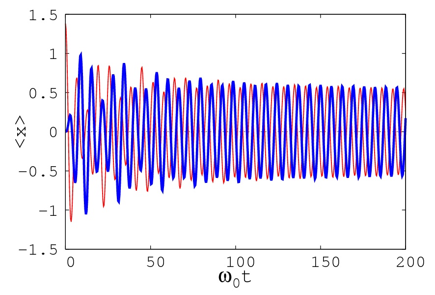
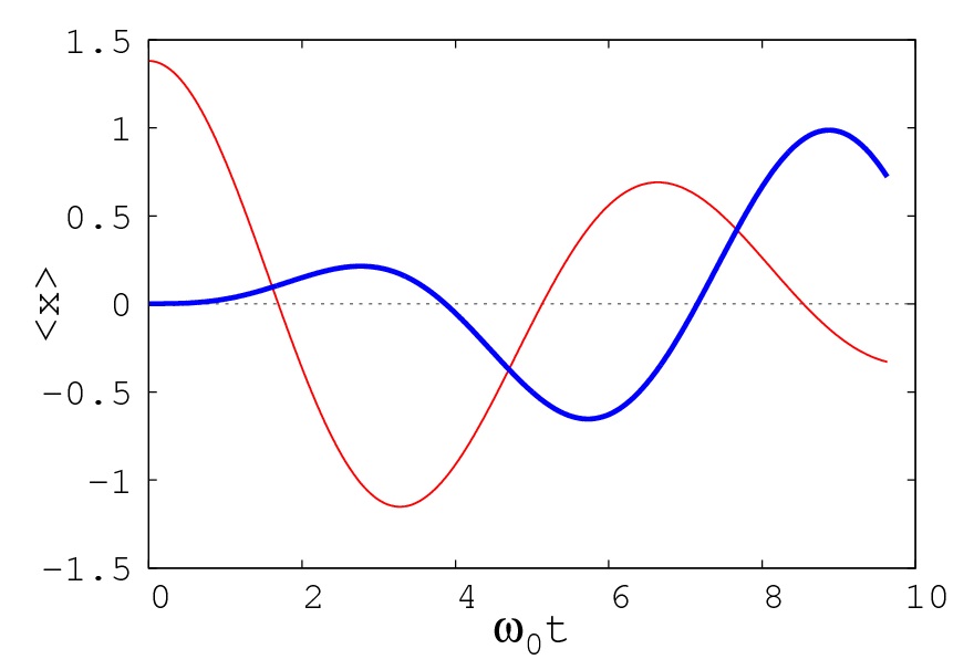
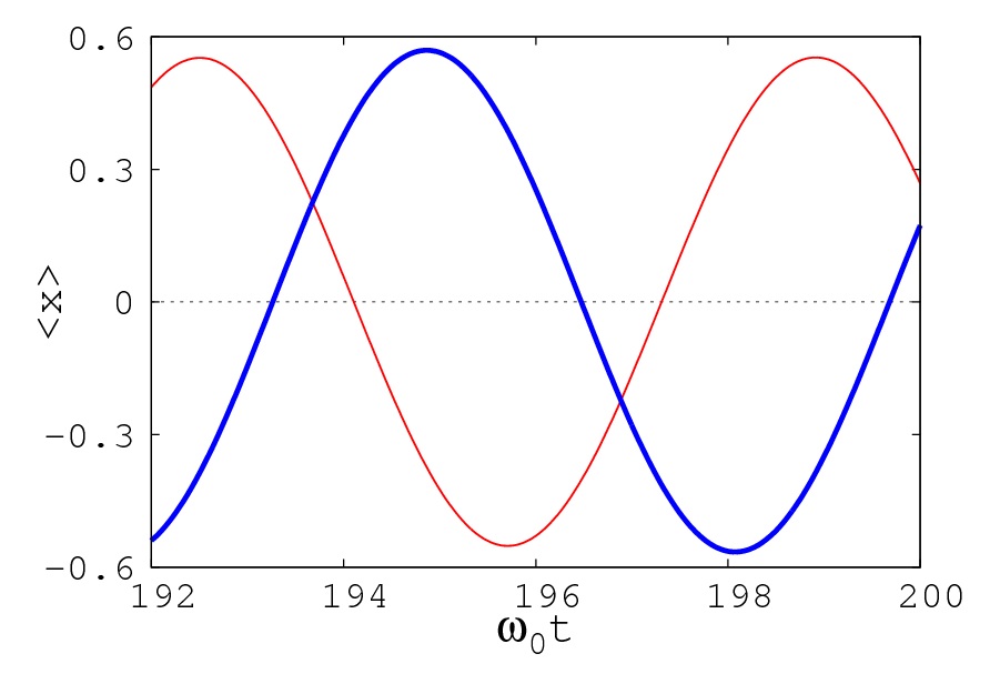
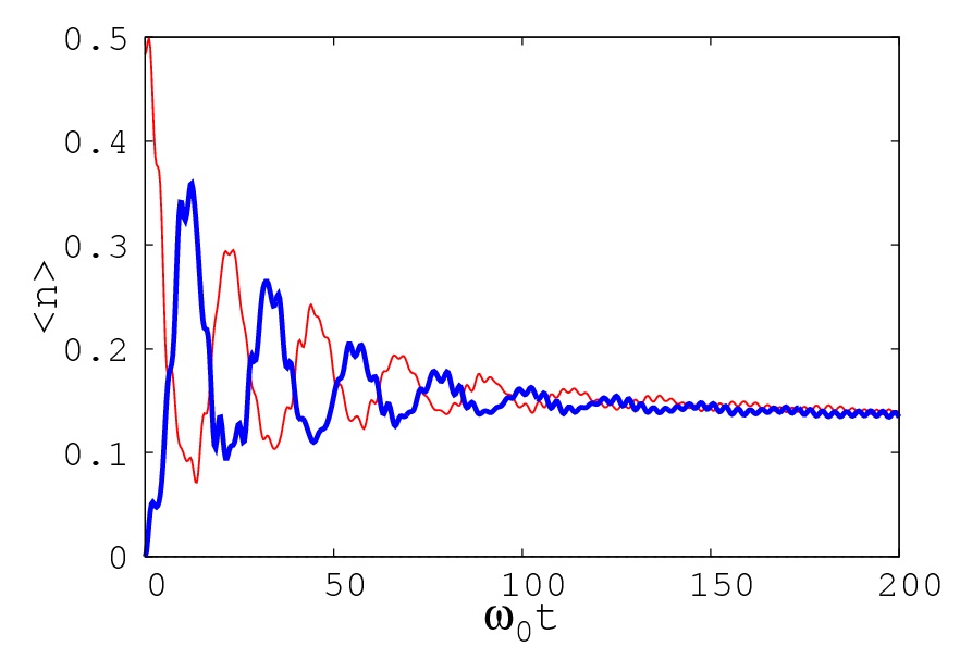
Figure 1: (Color online) . Evolution of the system when the oscillator 1 is prepared in a coherent state with $\alpha_{1}=0.7$ and the oscillator 2 is in the ground state; the TLS is in the state $\left|-\right\rangle$. The relevant parameters are: $\omega_{1}/\omega_{0}=0.95$, $\omega_{2}/\omega_{0}=1.01$, $g_{1}/\omega_{0}=0.2$, $g_{2}/\omega_{0}=0.21$, $\Gamma/\omega_{0}=0.1$, $\theta_{1}=0$, $\theta_{2}=\pi/4$. We show the behavior of $\langle x_{1}\rangle$ (thin red line) and $\langle x_{2}\rangle$ (bold blue line), in a wide range (a), for short time (b) and in the final part of the considered interval of time (c). It is clear that in the beginning the expected values of the positions oscillate with different frequencies, while in the final part of the evolution they oscillate with the same frequency but with a phase difference which is equal to $\pi-(\theta_{2}-\theta_{1})=3\pi/4$, as expected from the theory. In (d) it is also shown the average number of excitations in each oscillator.

The results predicted by the previous theoretical analysis are confirmed by our numerical simulations, which have been developed considering a zero-temperature reservoir whose action is described by the phenomenological model in (13). In Fig.1 we show the dynamics of the system when one of the two oscillators is prepared in a coherent state (with a small number of average excitations, in order to make possible truncation of the Hilbert space at a reasonable point), the other oscillator is in its vacuum and the TLS is in its ground state. We consider the expectation values of the two positions $\langle x_{1}\rangle$ and $\langle x_{2}\rangle$ in (a), (b) and (c), and the average values of excitations $\langle n_{1}\rangle$ and $\langle n_{2}\rangle$ in (d). It is well visible that after a certain time the dynamics stabilizes, both in terms of amplitudes of the oscillations of the positions (see (a)) and in terms of average numbers of excitations (see (d)). A closer look at short-time and long-time dynamics ((b) and (c), respectively) shows that the positions initially oscillate with different frequencies, while end up to oscillate at the same frequency and with a phase difference which is $3\pi/4$, as expected from the theoretical analysis, for the specific values of the parameters.

In Fig.2 we find that the final situation can be different (oscillations with the same frequency but phase differences equal to $0$ or $\pi$), depending on the parameters.

Observe that in all such pictures the asymptotic oscillations have almost the same amplitude. This is due to the fact that we have $g_{1}/g_{2}\approx 1$, so that $\gamma\approx\pi/4$ (see (21c)-(21d)). For the same reason, the amplitudes of asymptotic oscillations of the two modes are predicted to be essentially one half of the amplitude of the initial oscillation of oscillator $1$ (see (33a)-(33b)), which is well visible in Fig.1a.

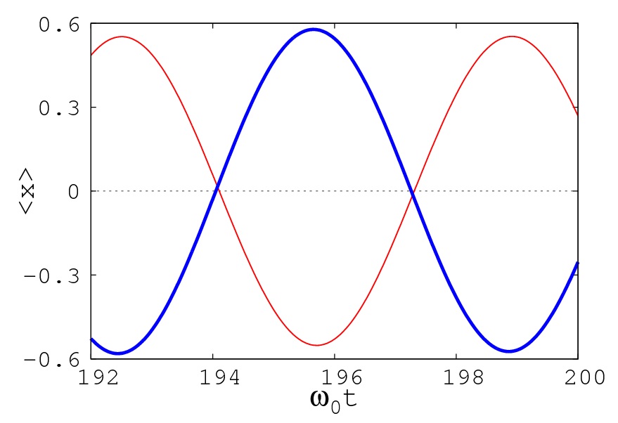
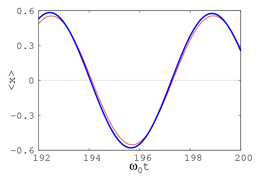
Figure 2: (Color online) . Asymptotic single-frequency evolution of the expectation values of the positions, with opposite phases (a) and the same phase (b). The relevant parameters are: $\alpha_{1}=0.7$, $\omega_{1}/\omega_{0}=0.95$, $\omega_{2}/\omega_{0}=1.01$, $g_{1}/\omega_{0}=0.2$, $g_{2}/\omega_{0}=0.21$, $\Gamma/\omega_{0}=0.1$. In (a) we have $\theta_{1}=0$, $\theta_{2}=0$, while for (b) it is $\theta_{1}=0$, $\theta_{2}=\pi$. Thin red line for the oscillator 1 and bold blue line for oscillator 2.

V Generalizing the Model

We can try to generalize the result obtained with a single TLS, by using $M$ TLSs, each one ‘killing’  a specific linear combination of the bare modes. Consider the following Hamiltonian:

$$H_{\mathrm{S}} = \sum_{k=1}^{N}\omega_{k}a^{\dagger}_{k}a_{k}+\sum_{j=1}^{M}\frac{\omega_{0}}{2}\sigma_{z}^{j}$$ (34)

$$+ \sum_{j=1}^{M}\sum_{k=1}^{N}g_{jk}(\mathrm{e}^{\mathrm{i}\theta_{jk}}a_{k}+\mathrm{e}^{-\mathrm{i}\theta_{jk}}a_{k}^{\dagger})\sigma_{x}^{j}\,.$$

The following linear combinations of the bare modes are involved in the interaction with the leaking TLSs:

$$c_{j}=G^{-1}\sum_{k=1}^{N}g_{jk}\mathrm{e}^{\mathrm{i}\theta_{jk}}a_{k}\,,\qquad j=1,...,M\,.$$ (35)

with $G=\sqrt{\sum_{j}|g_{j}|^{2}}$.

In general, they are not independent, but they can be generated as linear combinations of $M$ independent modes. Let us call $\bar{c}_{i}$, $i=1,...,N$, $N$ independent modes such that $\bar{c}_{N-M+1},...,\bar{c}_{N}$, suitably combined, generate $c_{1},...,c_{M}$. The remaining $N-M$ modes, $\bar{c}_{1},...,\bar{c}_{N-M}$, are not coupled to the TLSs.

After a while, the modes related to $\bar{c}_{N-M+1},...,\bar{c}_{N}$ will waste all their energy and the dynamics will be associated only to the modes $\bar{c}_{1},...,\bar{c}_{N-M}$. If the frequencies of the surviving modes are very close, the $N$ oscillators constituting the system will essentially evolve with a single frequency.

As a specific example, consider $N$ oscillators and $M=N-1$ dissipating two-level systems, and assume that each couple of adjacent oscillators is coupled to one of the TLS (see the scheme in Fig.3). In particular, consider the following Hamiltonian:

$$H_{\mathrm{S}} = \sum_{k=1}^{N}\omega_{k}a^{\dagger}_{k}a_{k}+\sum_{j=1}^{N-1}\frac{\omega_{0}}{2}\sigma_{z}^{j}$$ (36)

$$+ \sum_{j=1}^{M}g_{j}(a_{j}-a_{j+1}+h.c.)\sigma_{x}^{j}\,.$$

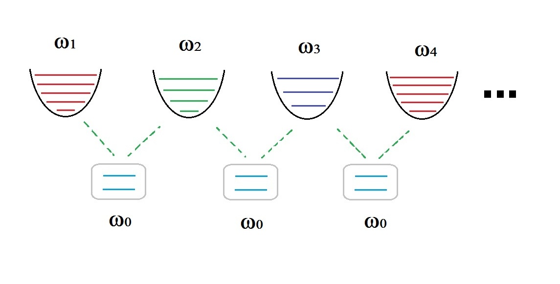
Figure 3: (Color online). A chain of $N$ oscillators coupled to a chain of $N-1$ TLSs.

It is easy to see that it turns out that the mode $a=(a_{1}+a_{2}+\cdots+a_{N})/\sqrt{N}$ is protected, while the $N-1$ modes $(a_{1}-a_{2})/\sqrt{2}$, $(a_{2}-a_{3})/\sqrt{2}$,…, $(a_{N-1}-a_{N})/\sqrt{2}$ (which are not independent from each other, but are all independent from $a$ and can be rearranged to form a set of $N-1$ independent modes) are leaking. Then, after a while, only mode $a$ will survive and we will observe a collective motion with a single frequency and all the oscillators with definite phase difference.

VI Conclusions

In this paper we have considered the occurrence of synchronization of harmonic oscillators induced by two-level systems. Because of the mixed algebra involving creation/annihilation operators on one side and Pauli operators on the other side, it is not possible to perfectly decouple the modes of the two oscillators from each other and, at the same time, one of them from the TLS. Nevertheless, we have introduced a new picture, that we address ‘single leaking mode picture’, where the two (transformed) modes are almost decoupled from each other (provided a certain condition is satisfied), and one of them is perfectly decoupled from the leaking two-level system. This circumstance allows us to forecast with a good degree of reliability that one of the two modes will lose energy, approaching the ground state, while the other will evolve unitarily. This will produce, in the original (Schrödinger) picture a collective oscillatory motion characterized by a single frequency.

Our predictions based on the Hamiltonian model of the system are corroborated by numerical results that show, in a clear way, not only the incoming of a single frequency, but also specific phase relations between the motions of the two oscillators predicted by our theoretical analysis. Such phase relation is very easily connected with the coupling constants ($g_{k}$’s) of the oscillators with the TLS, when the system is prepared in a single-mode coherent state. Even the amplitude of the oscillation of the position is put in connection with both the relevant parameters and the initial condition in a clear and simple way. Our theoretical analysis provides also general expressions valid for an arbitrary initial condition. A merit of our approach is that, in spite of the semi-qualitative nature of our analysis (in the sense that the dissipative dynamics is not solved or studied in detail), it enables us to make quantitative predictions about the joint frequency, individual amplitudes and phases of the synchronized motions.

Finally, in sec.V we have provided a generalization of the model involving $N$ oscillators and $M(<N)$ TLSs. By tuning the coupling constants between oscillators and leaking TLSs it is possible to induce synchronization of all the $N$ oscillators.

VII Acknowledgements

H. N. was supported by the Waseda University Grant for Special Research Projects (No. 2016B-173).

References

- (1) A. Pikovsky, M. Rosenblum, and J. Kurths, Synchronization: A Universal Concept in Nonlinear Sciences, Cambridge Nonlinear Science Series (Cambridge University Press, (2003).
- (2) Juan A. Acebrón, L. L. Bonilla, Conrad J. P rez Vicente, F lix Ritort, Renato Spigler, Rev. Mod. Phys., 77, 137 (2005).
- (3) M. Maianti, S. Pagliara, G. Galimberti and F. Parmigiani, Am. J. Phys. 77,834 (2009).
- (4) J. Pantaleone, Am. J. Phys. 70, 992 (2002).
- (5) S. H. Strogatz and I. Stewart, Scientific American 269 (6), 102 (1993).
- (6) L. Angelini,G. Lattanzi, R. Maestri, D. Marinazzo, G. Nardulli, L. Nitti, M. Pellicoro, G. D. Pinna, and S. Stramaglia, Phys. Rev. E 69, 061923 (2004).
- (7) Alex Arenas, Albert Diaz-Guilera, Jurgen Kurths, Yamir Moreno, Changsong Zhou, Physics Reports, 469, 93-153 (2008).
- (8) E. Padmanaban, Stefano Boccaletti, and S. K. Dana, Phys. Rev. E 91, 022920 (2015).
- (9) I. Hermoso de Mendoza, L. A. Pachon, J. Gomez-Gardenes and D. Zueco, Phys. Rev. E 90, 052904 (2014).
- (10) G. Manzano, F. Galve, G. L. Giorgi, E. Harn ndez-Garcia and R. Zambrini, Sc. Rep. 3, 1439 (2013).
- (11) G. L. Giorgi, F. Galve, G. Manzano, P. Colet and R. Zambrini, Phys. Rev. A 85, 052101 (2012).
- (12) F. Galve, G. L. Giorgi, and R. Zambrini, Phys. Rev. A 81, 062117 (2010).
- (13) D. M. Abrams and S. H. Strogatz, Phys. Rev. Lett. 93, 174102 (2004).
- (14) A. Mari, A. Farace, N. Didier, V. Giovannetti and R. Fazio, Phys. Rev. Lett. 111, 103605 (2013).
- (15) V. Ameri, M. Eghbali-Arani, A. Mari, A. Farace, F. Kheirandish, V. Giovannetti and R. Fazio, Phys. Rev. A 91, 012301 (2015).
- (16) M. R. Hush, Weiben Li, S. Genway, I. Lesanovsky and A. D. Armour, Phys. Rev. A 91, 061401(R) (2015).
- (17) G. L. Giorgi, F. Plastina, G. Francica, and R. Zambrini, Phys. Rev. A 88, 042115 (2013).
- (18) B. Zhu, J. Schachenmayer, M. Xu, F. Herrera, J. G. Restrepo, M. J. Holland, and A. M. Rey, New J. Phys. 17, 083063 (2015).
- (19) B. Bellomo, G. L. Giorgi, G. M. Palma, R. Zambrini, Phys. Rev. A 95, 043807 (2017).
- (20) Wenlin Li, Chong Li, and Heshan Song, Phys. Rev. E 93, 062221 (2016).
- (21) Wenlin Li, Chong Li, and Heshan Song, Phys. Rev. E 95, 022204 (2017).
- (22) F. Bemani, Ali Motazedifard, R. Roknizadeh, M. H. Naderi, and D. Vitali, ArXiv:1703.01783.
- (23) Haibo Qiu, Roberta Zambrini, Artur Polls, Joan Martorell, and Bruno Juliá-Díazand, Phys. Rev. A 92, 043619 (2015).
- (24) V. Zhirov and D. L. Shepelyansky, Phys. Rev. Lett. 100, 014101 (2008).
- (25) O. Astafiev, K. Inomata, A. O. Niskanen, T. Yamamoto, Yu. A. Pashkin, Y. Nakamura and J. S. Tsai, Nature (London) 449, 588 (2007).
- (26) Th. K. Mavrogordatos, G. Tancredi, M. Elliott, M. J. Peterer, A. Patterson, J. Rahamin, P. J. Leek, E. Ginossar and M. H. Szymanska, Phys. Rev. Lett. 118, 040402 (2017).
- (27) H.-P. Breuer and F. Petruccione, The Theory of Open Quantum Systems (Oxford University Press, Oxford, UK, 2002).
- (28) C. W. Gardiner and P. Zoller, Quantum Noise (Springer, Berlin, 2000).
- (29) M. Scala, B. Militello, A. Messina, J. Piilo, and S. Maniscalco, Phys. Rev. A 75, 013811 (2007); M. Scala, B. Militello, A. Messina, S. Maniscalco, J. Piilo, and K.-A. Suominen, ibid. 77, 043827 (2008).
- (30) M. Scala, B. Militello, A. Messina and N. V. Vitanov, Phys. Rev. A 84, 023416 (2011); B. Militello, K. Yuasa, H. Nakazato, A. Messina, Phys. Rev. A 76, 042110 (2007); B. Militello, M. Scala and A. Messina A, Phys. Rev. A 84, 022106 (2011); B. Militello B, Phys. Rev. A 85, 064102 (2012).
- (31) F. Beaudoin, J. M. Gambetta, and A. Blais, Phys. Rev. A 84, 043832 (2011).
- (32) G. Zhang and H. Zhu, Sc. Rep. 5, 08756 (2015).
- (33) C. Davis-Tilley and A. D. Armour, Phys. Rev. A 94, 063819 (2016).