Time in dissipative tunneling: subtleties and applications

Abstract

Characteristic features of tunneling times for dissipative tunneling of a particle through a rectangular barrier are studied within a semiclassical model involving dissipation in the form of a velocity dependent frictional force. The average dwell time and traversal time with dissipation are found to be less than those without dissipation. This counter-intuitive behaviour is reversed if one evaluates the physically relevant transmission dwell time. Apart from these observations, we find that the percentage of energy lost by the tunneling particle is higher for smaller energies. The above observations are tested and confirmed in a realistic case by applying the dissipation model to study the current-voltage data in a Al/Al₂O₃/Al solid state junction at various temperatures. The friction coefficient for Al₂O₃ as a function of temperature is presented. It is found to decrease with increasing temperature.

I A brief history of tunneling time

Quantum tunneling was one of the first bizarre implications of quantum mechanics which at first found its application in the study of alpha decay of radioactive nuclei gamow . It was however soon realized that this phenomenon was not restricted to nuclear physics but was rather a general result of quantum mechanics which is now often used in atomic physics atomic , solid state physics weAPL , chaotic scattering chaos , in constructing electron tunneling microscopes and even in branches of science other than physics. Though we are a long way from 1928 when Gamow published his pioneering work gamow and tunneling seems to be a well understood phenomenon with ramifications in many branches of physics, there still exist paradoxes and unanswered questions in this field. For example, the time spent by a particle tunneling a barrier has been a topic of much debate with many different definitions of tunneling times in literature mugabooks ; haugereview ; winreport ; buettiker . In haugereview the authors discussed several time concepts such as the dwell time smith , traversal time buetikprl , phase time wigner and even complex times. Ref. bertulani discusses the tunneling of composite particles, resonant tunneling and how the coupling between intrinsic and external degrees of freedom can affect tunneling probabilities. The dwell time formalism for the transition from a quasilevel to a continuum of states was discussed in the context of electron and alpha particle tunneling in price . Over the years, many of the time concepts have been put to test in physical situations and the transmission dwell time seems to emerge as the concept with a physical meaning weAPL ; weEPL ; wetimedelay as well as free of paradoxes gotoiwamoto and singularities such as those found in the phase time meprl .

Dissipative tunneling times have however been explored to a lesser extent historically. In recent years, the authors in bhataroyAMP have studied the phase and dwell times with dissipation in different contexts bhataroy2 . In bhataroyAMP , studying the dissipative tunneling through an inverted harmonic oscillator in context with ion transport at nanoscale, the authors showed that the phase time delay can be estimated directly in terms of a frictional coefficient. The average dwell time, $\tau_{D}$, through a rectangular potential barrier using a path decomposition technique was investigated in konno leading to the counter-intuitive result that $\tau_{D}$ in the presence of dissipation becomes smaller than that in a non-dissipative case. The traversal time behaviour for a rectangular barrier with energy losses included was described in ranfagni within a semiclassical approach with dissipation included in the form of a frictional force. Using a somewhat similar approach for dissipation with the latter given by a frictional force as in buetikprl , in the present work we shall show that the counter-intuitive result found in konno can indeed be explained.

An understanding of the tunneling times with dissipation can prove important for studying the characteristics of solid state tunnel junctions. The importance of the tunneling times in this context was realized in schnupp where the author noticed that “the image force acting on an electron tunneling through a dielectric film enclosed by metal electrodes depends on the dielectric constant of the film and the charge build-up in the electrodes which in turn are both dependent on the duration of the tunneling process”. In what follows, we shall present the expressions for the dwell and traversal times with dissipation for tunneling through a rectangular barrier. Calculations using these expressions are done in context with an experiment weAPL reported in an earlier work by two authors of the present work. Ref. weAPL presented a method to extract the average dwell times from tunneling experiments in solid state junctions. The current-voltage (I-V) characteristics reported there are now used in a model that includes the effects of dissipation on tunneling times. Furthermore, the new fits to these data allow us to determine the frictional coefficient for Al₂O₃ from 3.5 to 300 K.

II Semiclassical Dwell and traversal times

The concept of an average dwell time was first introduced in the form of a collision time by Smith smith . Calling it as the time of residence in a region and using steady state wave functions he defined it as the integrated density divided by the flux in (or out). The lifetime of an unstable state was thereby given as the difference between the residence time with and without interaction. This difference was essentially the time delay introduced due to the formation, propagation and decay of the unstable state. Using the residence or dwell time delay, he went on further to construct a lifetime matrix, Q, which was Hermitian and the diagonal elements $q_{ii}$ gave the lifetimes of unstable states or resonances. The physical relevance of the residence time delay (or dwell time delay) as well as its relation with the phase time delay introduced earlier by Wigner and Eisenbud wigner became evident in wetimedelay and motivated further investigations of the same in multichannel scattering ourpra . The extraction of resonances from multichannel scattering data is an involved task and we refer the reader to workman for details. Time delay can also be negative and interesting interpretations of time advancements can be found in timeadv . Many years after Wigner, Smith and Eisenbud’s papers, the dwell time in one-dimension was revisited by Büttiker buettiker in relation with the newer concepts of Larmor time and traversal time.

Given an arbitrary barrier $V(x)$ in one-dimension, for a particle of mass $m$ confined to an interval $(x_{1},x_{2})$, the average dwell time which is defined as the ratio of the density to flux can be written within the semiclassical Jeffreys-Wentzel-Kramers-Brillouin (JWKB) approximation as weEPL ,

$$\tau_{D}(E)\,=\,{m\over\hbar}\,\int_{x_{1}}^{x_{2}}\,{dx\over\kappa(x)}\,{\rm exp}\,\biggl{[}-2\,\int_{x_{1}}^{x}\,dx^{\prime}\,\kappa(x^{\prime})\biggr{]}\,,$$ (1)

where, $\kappa(x)\,=\,{\sqrt{2\,m\,(V(x)\,-\,E)}/\hbar}$ for tunneling at energies, $E$, below the top of the barrier. Defining an effective velocity, $v(x)=\hbar\kappa(x)/m$, the traversal time which comes closer to the classical definition of a particle “traversing” a barrier is given by,

$$\tau_{tr}=\int_{x_{1}}^{x_{2}}\,{m\over\hbar\kappa(x)}\,dx\,=\,\int_{x_{1}}^{x_{2}}\,\biggl{[}{m\over 2(V(x)-E)}\biggr{]}^{1/2}\,dx\,.$$ (2)

Improved JWKB near the base of the barrier

The JWKB approximation is known to be reasonably good away from the lower and upper extremes of the potential barrier. There exist different prescriptions to improve the JWKB formulae near the top as well as the bottom of the barrier weWKB . In the present section, however, we shall consider a method to improve the JWKB dwell time only near the base of the barrier for reasons which are explained briefly in the paragraph below.

Dissipative effects in the present work are included by introducing a damping force which causes a loss of energy of the tunneling particle. In the next section, we will see that the damping force is proportional to the velocity of the incoming particle. In a rectangular barrier of height $V_{0}$, the effective velocity, $v(x)=\hbar\kappa(x)/m$ becomes, $v_{0}=[2(V_{0}-E)/m]^{1/2}$. Thus, inside the tunnel barrier the effective velocity decreases with increasing energy. Since it approaches zero near the top of the barrier, the energy loss is greater for particles with smaller energies relative to the barrier height. Therefore, to include dissipative effects, the lowest energies (at the base of the barrier) are the most important in the improvement of the JWKB formula. With this aim we use the prescription given in [27], for the JWKB wave function, in order to improve the dwell time given in Eq. (1) within the JWKB approximation.

In eltWKB , the authors used a generalization of the JWKB connection formulas to derive expressions of the transition amplitudes which behave correctly at the bottom of the barrier. The procedure effectively involved the introduction of a multiplicative factor into the normalization of the JWKB wave function. Details of the approach with a wide range of examples are given in a more recent review article friedrichrep . Here, we shall breifly explain the derivation of this factor. The authors begin by examining the connection formulas at the classical turning point ($x_{t}$), which for example, in the most general case can be written as,

$${2\over\sqrt{\kappa(x)}}\cos{\biggl{(}{1\over\hbar}\biggl{|}\int_{x_{t}}^{x}\,\kappa(x^{\prime})dx^{\prime}\biggr{|}\,-\,{\phi\over 2}\biggr{)}}\leftrightarrow{N\over\sqrt{\kappa(x)}}\,\exp{\biggl{(}-{1\over\hbar}\biggl{|}\int_{x_{t}}^{x}\kappa(x^{\prime})dx^{\prime}\biggr{|}\biggr{)}}$$

where $\kappa(x)=\sqrt{|2m(V(x)-E)|}$ and the two parameters $N$ and $\phi$ are determined by comparing the exact solution corresponding to an exponentially decreasing wave on the classically forbidden side with the oscillating JWKB waves on the allowed side. The connection formulas in conventional semiclassical theories are derived assuming that the potential is a linear function of $x$ in the vicinity of $x_{t}$ and this region extends “sufficiently far” which eventually leads to $\phi=\pi/2$ and $N=1$. Among several examples, the authors consider the case of a rectangular barrier of height $V_{0}$ and note that the potential appears to be a sharp step at each of the two turning points in the rectangular barrier. The amplitude factor $N$ and phase $\phi$ are obtained by comparing the JWKB waves on either side of a turning point with the exact wave function for a sharp potential step of height $V_{0}$. The result is $N=2\sqrt{{k\kappa_{0}/k^{2}+\kappa_{0}^{2}}}$ with $k=\sqrt{2mE}$ and $\kappa_{0}=\sqrt{2m(V_{0}-E)}$. Such an amplitude factor improves the transmission coefficient calculated in the JWKB approximation and brings it quite close to the exact one. An example of such an improvement can be seen in Fig. 8 of Ref. friedrichrep .

The average dwell time given in Eq. (1) is evaluated using the standard definition weEPL , namely, $\tau_{D}(E)=\int_{x_{1}}^{x_{2}}\,{|\Psi(x)|^{2}/j}$ where $j=\hbar\kappa(x)/m$ (with $\kappa(x)=\sqrt{2m(V(x)-E)}$) and $\Psi(x)$ is replaced by the JWKB wave function $\Psi(x)=\exp{[-2\int_{x_{1}}^{x}dx^{\prime}\kappa(x^{\prime})]}$. If we introduce the improved wave function as discussed above, i.e., $\Psi(x)=N\,\exp{[-2\int_{x_{1}}^{x}dx^{\prime}\kappa(x^{\prime})]}$, with $N$ as given above, the average dwell time for a rectangular barrier changes to $\tau_{D}^{\rm improved}=N^{2}\tau_{D}$. The inclusion of dissipation in the present work changes the rectangular barrier with height $V_{0}$ to $V(x)=V_{0}+\eta v_{0}x$. The additional term with $\eta$ is a small perturbation to the rectangular barrier and hence we assume the factor $N$ for the barrier $V(x)$ to be the same as that in the case of a rectangular barrier and evaluate $\tau_{D}^{\rm improved}$ as above. In Fig. 1, we see a comparison between the average dwell times $\tau_{D}$ without dissipation, evaluated exactly for a rectangular barrier buettiker (solid line), in the JWKB (dashed line) and the improved JWKB (dash dotted line) which almost coincides with the exact expression for all energies except ones close to the top of the barrier. Notice that in contrast to the exact $\tau_{D}$, one evaluated in the JWKB does not approach zero for energies at the bottom of the barrier. The improved JWKB expression takes care of this deficiency and agrees with the exact $\tau_{D}$.

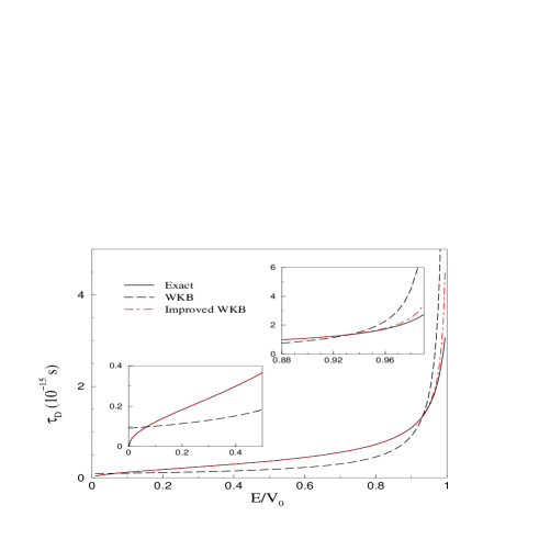
Figure 1: Average dwell time, $\tau_{D}$, without dissipation for a rectangular barrier of height $V_{0}$. Solid line is the exact expression as in buettiker , dashed line is $\tau_{D}$ within the JWKB approximation and dash-dotted line is $\tau_{D}^{\rm improved}$ (see text).

III Dissipation in tunneling

The question, “what is the effect of dissipation on tunneling?”, was put forth in a seminal paper by Caldeira and Leggett caldeira in 1983 where the authors started with a damped equation of motion for the system as follows:

$$m\ddot{x}\,+\,\eta\dot{x}\,+\,{\partial V\over\partial x}\,=\,F_{ext}\,.$$ (3)

The potential $V(x)$ and friction coefficient $\eta$ were regarded as experimentally determined quantities. Dissipative tunneling was later investigated by Ford et al. ford , using a quantum Langevin approach. The effect of dissipation has been studied in literature along two different lines: phenomenological approaches and microscopic formulations where dissipation comes about due to the coupling of the system to a heat bath of infinitely many degrees of freedom. In the present work we restrict ourselves to the former type of approaches. We study the effects of dissipation in a solid state junction with an electron traversing through a metal - insulator - metal surface, within a model which is conceptually similar to that in caldeira and consider a frictional force of the type $F(x)=\eta v(x)$, where, $v(x)$ is the effective velocity defined above (however, now with dissipation) and $\eta$ is the coefficient of friction. Such a model was proposed in buetikprl and often used to represent the dissipation due to a damping force. Though in the microscopic treatments, dissipation is included by considering the entanglement of the system and the environment in a time dependent quantum mechanical approach qmdisip , we restrict here to the simpler approach involving a frictional coefficient due to the following reasons: (i) the objective of the present work is to explore the behaviour and subtleties of the dwell times and traversal times which are concepts involving stationary wave functions. These concepts give a measure of time intervals without refering to the parametric time $t$ appearing for example in the time dependent Schrödinger equation. (ii) The question which we wish to address in the present work is “how does such a stationary time concept get affected by dissipation of the particle energy during tunneling”? and not a more global one of how the quantum tunneling is affected by the interaction with the environment which produces the dissipation. Such a semiclassical approach has also been used earlier in buetikprl ; ranfagni2 ; bhataroyadmp . We also refer the reader to pimpale for a review on the various approaches.

The introduction of the frictional force, $\eta\dot{x}$, is not entirely arbitrary but can rather be derived under certain approximations from the complete picture of a system coupled with an environment ingold ; weissetc . The author in ingold for example, starts with a model for the dissipative quantum system by considering a Hamiltonian with three contributions coming from the system degrees of freedom, the environment and the coupling between them. The system Hamiltonian models a particle of mass $m$ moving in a potential $V$ and the environment Hamiltonian describes a collection of harmonic oscillators. After some discussions and algebra, the author arrives at an equation of motion given by,

$$m\ddot{x}\,+\,m\displaystyle\int_{0}^{t}\,ds\,\gamma(t-s)\,\dot{x}(s)\,+\,{\partial V\over\partial x}\,=\,F_{ext}(t),$$ (4)

where $\gamma(t)$ is a damping kernel which can be expressed in terms of the spectral density, $J(\omega)$, of bath oscillators as,

$$\gamma(t)={2\over m}\displaystyle\int_{0}^{\infty}\,{d\omega\over\pi}\,{J(\omega)\over\omega}\,\cos{(\omega t)}\,.$$ (5)

The most frequently used spectral density, $J(\omega)=m\eta\omega$, associated with the so called “Ohmic damping”, then leads us back to Eq. (3) of Caldeira and Leggett, mentioned above.

For a particle with energy $E$, tunneling a rectangular barrier of width $L$ and height $V_{0}$, the amount of energy lost while traversing a distance $x$ can be written as, $\Delta E(x)=\eta\int_{0}^{x}\,v(x^{\prime})dx^{\prime}=\eta[2(V_{0}-E)/m]^{1/2}\,x$. This implies that at every $x$ inside the barrier, the energy of the particle is modified from $E\to E^{\prime}=E-\Delta E(x)$ and $\kappa_{0}\,=\,{\sqrt{2m\,(V_{0}\,-\,E)}/\hbar}$ in turn is modified to $\kappa(x)\,=\,{\sqrt{2m\,(V_{0}\,-\,E\,+\,\Delta E(x))}/\hbar}$. The maximum energy lost, $\Delta E(L)$, however, cannot exceed the energy of the tunneling particle, i.e., $\Delta E(L)\leq E$. This puts a limit on the allowed value of the friction coefficient and we get, $\Delta E(L)=\eta_{max}\,[2(V_{0}-E)/m]^{1/2}\,L=E$, leading to,

$$\eta_{max}={V_{0}\over L}\,\biggl{(}{E\over V_{0}}\biggr{)}\,\Bigg{[}{m\over 2V_{0}\biggl{(}1-{E\over V_{0}}\biggr{)}}\Bigg{]}^{1/2}\,.$$ (6)

In Fig. 2, we show the fraction of energy lost as a function of the energy of the tunneling particle for a couple of values of $\eta$ which are close to those determined in a realistic tunneling of an electron in a solid state junction (to be discussed in the next section).

Figure 2: Fraction of energy lost as a function of energy of the tunneling particle.

III.1 Average dwell time and traversal time with dissipation

Defining, $V_{0}+\Delta E(x)=V(x)$, gives $\kappa(x)\,=\,{\sqrt{2\,m\,(V(x)\,-\,E)}/\hbar}$ and the dwell and traversal times with dissipation for a rectangular barrier can be evaluated within the JWKB approximation, using Eqs (1) and (2) for tunneling of a particle with energy $E$ through a potential barrier given by $V(x)$. The calculation is easily performed numerically. However, to get some insight into the relations, let us consider the tunneling of particles with a small amount of dissipation, such that, $\Delta E(x)\ll V_{0}-E$ and hence $\hbar\kappa(x)$ can be expressed approximately as, $\hbar\kappa(x)=\hbar\kappa_{0}+\eta\,x$. Assuming further that, $\eta L\ll\hbar\kappa_{0}$, the average dwell time reduces to a rather simple expression given by (see appendix for details)

$$\tilde{\tau}_{D}={m\over 2\,\hbar\kappa_{0}^{2}}\,\biggl{[}\,1\,-\,\exp^{-2\,\kappa_{0}\,L\,-\,\eta\,L^{2}/\hbar}\,\biggl{(}\,1-{2\eta L\over\hbar\kappa_{0}}\,\biggr{)}\,\biggr{]}.$$ (7)

The transmission coefficient with dissipation can similarly be shown to be

$$\tilde{\cal T}(E)=e^{-\eta L^{2}/\hbar}\,e^{-2\kappa_{0}\,L}\,,$$ (8)

where $e^{-2\kappa_{0}\,L}$ is the standard transmission coefficient in the JWKB approximation. The traversal time with dissipation, as shown in ranfagni reduces to

$$\tilde{\tau}_{tr}={m\over\eta}\,\ln\biggl{(}\,1\,+\,{L\over a}\,\biggr{)}\,,$$ (9)

with $a^{2}=2m(V_{0}-E)/\eta^{2}$, for $E<V_{0}$ as shown in ranfagni . In order to ensure the correct behaviour of the dwell time close to the bottom of the barrier, the dwell time in Eq. (7) is multiplied by the factor $N^{2}$ suggested in the previous section on the improved JWKB expressions.

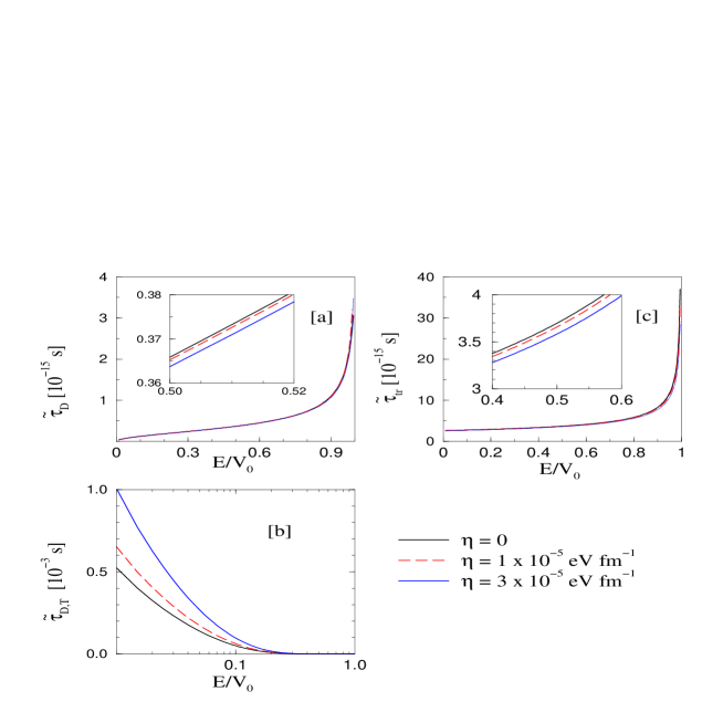
Figure 3: Average dwell time, $\tilde{\tau}_{D}$ [a], transmission dwell time, $\tilde{\tau}_{D,T}$ [b] and traversal time, $\tilde{\tau}_{tr}$ [c] for different amounts of dissipation in tunneling through a rectangular barrier of height $V_{0}$=1.8 eV and length $L=20.8\textrm{\AA}$.

III.2 Reflection, Transmission and Average dwell time

The definition of an average dwell time, $\tau_{D}$, is the time spent in a region, say, $(x_{1},x_{2})$ regardless of the fact if the particle escaped by reflection or transmission. This $\tau_{D}={\int_{x_{1}}^{x_{2}}\,|\Psi(x)|^{2}\,dx/j}\,$ is defined nusen as the number density divided by the incident flux, namely, $j=\hbar\,k_{0}\,/\mu$ (with $k_{0}=\sqrt{2\mu E}/\hbar$) for a free particle. However, one can also define transmission and reflection dwell times for the particular cases when the particle, after dwelling in a region, escaped either by transmission or reflection. The flux $j$ in these cases would get replaced by the transmitted or reflected fluxes, $j_{T}=\hbar\,k_{0}{\cal T}/\mu$ and $j_{R}=\hbar\,k_{0}{\cal R}/\mu$ gotoiwamoto respectively. One would then obtain gotoiwamoto ,

$${1\over\tau_{D}}\,=\,{{\cal T}\over\tau_{D}}\,+\,{{\cal R}\over\tau_{D}}\,=\,{1\over\tau_{D,T}}\,+\,{1\over\tau_{D,R}}$$ (10)

where ${\cal T}$ and ${\cal R}$ are the transmission and reflection coefficients (with ${\cal T}\,+\,{\cal R}\,=\,1$ due to conservation of probability) and $\tau_{D,T}=\int|\Psi|^{2}dx/j_{T}$ and $\tau_{D,R}=\int|\Psi|^{2}dx/j_{R}$, define the transmission and reflection dwell times respectively. In Ref. weEPL , it was shown that it is the transmission dwell time, $\tau_{D,T}$ which can be attributed the physical meaning of the lifetime of a decaying nucleus. Within a semiclassical model for alpha particle tunneling, $\tau_{D,T}$ was shown to reproduce the half-lives of heavy nuclei. Defining a transmission dwell time in the case of dissipative tunneling in the same manner as above, we can write, $\tilde{\tau}_{D,T}(E)=\tilde{\tau}_{D}(E)/\tilde{{\cal T}}(E)$ where $\tilde{\tau}_{D}(E)$ and $\tilde{{\cal T}}(E)$ as defined in (7) and (8) are the average dwell time and transmission coefficient with dissipation. It is also worth mentioning that in gotoiwamoto it was shown that whereas the average dwell time saturates with increasing widths of a tunneling barrier (leading to speculations of superluminal propagation), the transmission dwell time does not. The latter was shown to simply increase with barrier width. Due to the fact that the transmission coefficient ${\cal T}$ is usually much smaller than ${\cal R}$, we have the average, $\tau_{D}\approx\tau_{D,R}$, i.e., the average dwell time is similar to the reflection dwell time and $\tau_{D,T}\gg\tau_{D,R}$. In the presence of dissipation, there is an energy loss and the transmission coefficient (calculated at a lower energy, $E-\Delta E$) is reduced and hence $\tilde{\tau}_{D,T}=\tilde{\tau}_{D}/\tilde{{\cal T}}$ increases. The reflection coefficient however, increases and hence the reflection dwell time $\tau_{D,R}$ and hence the average dwell time decrease. Thus, in what follows, we shall see that another paradoxical situation which arises from the calculation of the average dwell time is resolved if one rather studies the behaviour of the transmission dwell time.

In Fig. 3a, we show the average dwell time with and without dissipation for a typical example of electron tunneling through a solid state junction. The details of the dissipation constant and its values will be discussed in a later section. In the inset in Fig. 3a, we can see that the dwell time with dissipation is less than that without dissipation. The traversal time with dissipation (see Fig. 3c) displays a similar behaviour too. This counter-intuitive result is however reversed when we calculate the transmission dwell time and a particle losing energy is indeed seen to spend a greater amount of time in the barrier, in Fig. 3b. This observation once again confirms the physical nature of the transmission dwell time. Apart from this, we have also seen in Fig. 2 that the fraction of energy lost in the barrier decreases with increasing energy. As a result, the transmission dwell time, $\tilde{\tau}_{D,T}$, with dissipation can be seen in Fig. 3b to be similar to $\tau_{D,T}$ without dissipation for energies approaching the top of the barrier.

IV Temperature dependent dissipation in Al₂O₃

In an earlier paper weAPL involving two of the authors of the present work, measurements of the current-voltage (I-V) characteristics of an Al/Al₂O₃/Al junction at temperatures from 3.5 to 300 K were reported. These data were used in order to extract the temperature dependence of characteristic quantities such as the barrier height and the average dwell time in the tunneling of an electron through the Al/Al₂O₃/Al junction. The rectangular barrier height $V_{0}(T)$ was found to decrease for temperatures increasing from 3.5 to 300 K. In what follows, we shall try to relate the temperature dependence of $V_{0}(T)$ found in weAPL to the dissipation phenomenon and see if a correlation emerges. In the model of the present work, the problem of dissipative tunneling through a rectangular barrier of fixed height $V_{0}$ gets modified to that of tunneling of a particle with energy, $E$, through an effective potential $V(x)=V_{0}+\Delta E(x)$. If one starts with the assumption that the amount of energy dissipated in tunneling could change with temperature, i.e., $\Delta E(x)\to\Delta E(x,T)$, the effective potential can be expressed as,

$$V(x,T)=V_{0}\,+\,\eta(T)v_{0}x\,,$$ (11)

where, $\Delta E(x,T)=\eta(T)v_{0}x$ and the temperature dependence of the potential barrier is contained in the coefficient of friction, $\eta$. The transmission coefficient for a particle tunneling through the potential $V(x,T)$ is given by (8) with the difference that $\eta\to\eta(T)$. This means that the I-V data in weAPL which were fitted using the commonly used Simmons’ JWKB formula simmon , $J(V)=\int_{0}^{E_{m}}\,{\cal T}(E)\xi(V)\,dE$, with a transmission coefficient ${\cal T}(E)$, can now be fitted using the transmission coefficient with dissipation, namely, $\tilde{{\cal T}}(E)$ instead of ${\cal T}(E)$. Since $\tilde{{\cal T}}(E)$ in the JWKB approximation can be approximated (as shown in the appendix) for small amounts of energy dissipation by, $\tilde{{\cal T}}(E)=e^{-\eta(T)L^{2}/\hbar}{\cal T}(E)$, the current density $J(V)$ in Simmons’ model gets modified to,

$$\tilde{J}(V)=e^{-\eta(T)L^{2}/\hbar}\,\int_{0}^{E_{m}}\,{\cal T}(E)\xi(V)\,dE\,,$$ (12)

with the factor $\xi(V)$ as given in simmon . For a detailed derivation of the I-V relations (in the absence of dissipation) for low, intermediate and high voltages we refer the reader to the seminal papers of Simmons simmon and proceed here by noting that in case of dissipative tunneling, $J(V)$ in simmon simply gets modified to $\tilde{J}(V)=e^{-\eta(T)L^{2}/\hbar}\,J(V)$. Performing new fits to the I-V data with fixed barrier height, $V_{0}$, and fixed width, $L$, but the frictional coefficient $\eta$ as a free parameter which can vary with temperature, we find that the best fit is obtained for a constant barrier width and height of $L=20.8\textrm{\AA}$ and $V_{0}=1.799$ eV respectively. The latter is indeed the height of the barrier found in weAPL at 300 K. In Fig. 4a, we present the fitted values of $\eta$ as a function of temperature.

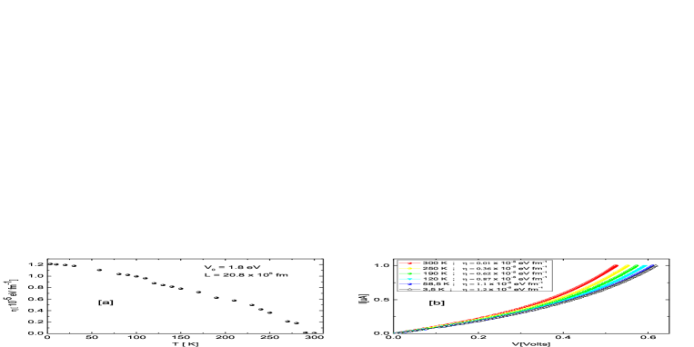
Figure 4: Dissipation coefficient, $\eta$ as a function of temperature [a] and the I-V characteristics (reported in weAPL and re-fitted here as explained in the text) at different temperatures [b] for electrons tunneling through a solid state junction of Al/Al₂O₃/Al.

We see a reduction in $\eta$ or a decrease in energy loss with increasing temperature. This behaviour is consistent with the results in weAPL , where performing a fit without taking dissipation into account, we found that the barrier height, $V_{0}(T)$, decreases with increasing temperature. A smaller $V_{0}$ for a given energy $E$ corresponds to the tunneling of the particle closer to the top of the barrier where the energy loss is little (see Fig. 2). It is interesting to note that the same I-V data (see Fig. 4b) can be fitted either with a model including dissipation where the coefficient of friction, $\eta(T)$, decreases with temperature for a fixed barrier height $V_{0}$ or with $\eta=0$ and a temperature dependent barrier height $V_{0}(T)$. Thus, in a model which includes dissipation explicitly, the effect of the temperature dependence of the barrier height is reflected in a temperature dependence of the friction coefficient.

V Summary

Dissipative tunneling of a particle such as an electron through a rectangular barrier has been investigated using the semiclassical JWKB approximation. Though the choice of an electron tunneling a rectangular barrier has been made in view of the analysis of the current-voltage data weAPL which is re-analysed here with dissipation, the characteristics of the dwell and traversal times found here should hold in general. The average dwell time of a particle tunneling a barrier (i.e., the time spent in a region irrespective of the fact if the particle got reflected or transmitted after residing in the barrier) is reduced in dissipative tunneling. This counter-intuitive result is however reversed if one evaluates the transmission dwell time and dissipation of energy in the barrier is found to delay the tunneling of the transmitted particles. Apart from this, the percentage energy loss in tunneling is found to be maximum near the base of the barrier and decreases for energies approaching the top of the barrier.

Based on the realistic example of an electron tunneling through a solid state junction, we find that the traversal time (as defined in (2)) is an order of magnitude larger than the average dwell time spent by the electron in the barrier. Given the reciprocal relation (Eq. (10)) for the average, transmission and reflected dwell times, the transmission dwell time comes out to be orders of magnitude larger than the average dwell time (shown in Fig. 3). Fits to the current voltage (I-V) data in the Al/Al₂O₃/Al junction for temperatures ranging between 3.5 K and 300 K, using the dissipation model of the present work display a decreasing dissipation (frictional) coefficient as a function of increasing temperature. The method may prove useful to study dissipative effects in junctions with other materials too.

Appendix A Dwell time with dissipation

Noticing that the effects of dissipation are mostly relevant at the base of the barrier, an expression for the dwell time with dissipation can be derived analytically within some reasonable approximations. We find that the difference between the numerical results presented in this work and those evaluated from the analytical expression as in Eq. (7) is negligible. Here we give a brief derivation of Eq. (7) and the transmission coefficient with dissipation in the JWKB.

The effective velocity for a particle tunneling a rectangular barrier of height $V_{0}$ can be written as $v_{0}=\hbar\kappa_{0}/m$, with

$$v_{0}=\frac{\hbar k}{m}=\sqrt[]{\frac{2}{m}\left(V_{0}-E\right)}\qquad\kappa_{0}=\frac{\sqrt{2m\left(V_{0}-E\right)}}{\hbar}$$

Including dissipation in the form of a frictional force, the energy loss can be given as a function of distance as, $\Delta E(x)=\eta\int_{0}^{x}v_{0}dx^{\prime}\,=\,\eta\sqrt{2(V_{0}-E)/m}\,x$. This means that $\kappa_{0}$ gets modified to $\kappa(x)$

$$\kappa_{0}\to\kappa(x) = \frac{\sqrt{2m(V_{0}-E^{\prime})}}{\hbar}$$

$$= \frac{\sqrt{2m\left[V_{0}-E+\Delta E(x)\right]}}{\hbar}$$

$$= \frac{\sqrt{2m(V_{0}-E)}}{\hbar}\left(1+\frac{\eta}{\hbar k}x\right)\quad;\quad\Delta E\ll V_{0}-E$$

$$\kappa(x) = \kappa_{0}\left(1+\frac{\eta}{\hbar k}x\right)$$ (13)

Replacing this expression of $\kappa(x)$ into Eq. (1), the average dwell time with dissipation is given as,

$$\tilde{\tau}_{D} = \frac{\mu}{\hbar}\int_{0}^{L}\frac{1}{k}\cdot exp\left(-2kx-\frac{\eta x^{2}}{\hbar}\right)dx-\frac{\eta\mu}{\hbar^{2}k^{2}}\int_{0}^{L}x\cdot exp\left(-2kx-\frac{\eta x^{2}}{\hbar}\right)dx$$ (14)

The above integral can be solved analytically using the following formulae:

$$\int exp\left(-ax-bx^{2}\right)dx = \frac{\sqrt{\pi}\cdot e^{a^{2}/4b}erf\left(\frac{a+2bx}{2\sqrt{b}}\right)}{2\sqrt{b}}$$

$$\int x\cdot exp\left(-ax-bx^{2}\right)dx = -\frac{a\sqrt{\pi}\cdot e^{a^{2}/4b}erf\left(\frac{a+2bx}{2\sqrt{b}}\right)}{4b^{3/2}}-\frac{e^{-x(a+bx)}}{2b}$$

After some lengthy but straightforward algebra, the expression in terms of the $erf$ functions can be further simplied by using the expansion, for $x\gg 1$,

$$erf(x)=1-\frac{e^{-x^{2}}}{\sqrt{\pi}x}\left[1-\frac{1}{2x^{2}}-\cdots\right]\,,$$ (15)

with the assumption that $\eta L\ll\hbar\kappa_{0}$. This leads us to the dwell time given in Eq. (7). The transmission coefficient in the JWKB, namely, $T=\exp{(-2\,\int_{0}^{L}\,\kappa(x)\,dx)}$, with $\kappa(x)$ defined as in (A) reduces to,

$$\tilde{T}(E) = \exp{(-2\int_{0}^{L}\,[\kappa_{0}+\eta x/\hbar]\,dx)}$$ (16)

$$= \exp{[-\eta L^{2}/\hbar]}\,{\cal T}(E)\,,$$

where ${\cal T}(E)=\exp{(-2\kappa_{0}L)}$, is the transmission coefficient without dissipation.

References

- (1) G. Gamow, Z. Phys. 51, 204 (1928).
- (2) G. Isić et al., Phys. Rev. A 77, 033821 (2008); W. O. Amrein and Ph. Jacquet, Phys. Rev. A 75, 022106 (2007); N. Yamanaka, Y. Kino, and A. Ichimura, Phys. Rev. A 70, 062701 (2004); Chun-Woo Lee, Phys. Rev. A 58, 4581 (1998).
- (3) E. J. Patiño and N. G. Kelkar, Appl. Phys. Lett. 107, 253502 (2015).
- (4) Yan V. Fyodorov and Hans-Jürgen Sommers, Phys. Rev. Lett. 76, 4709 (1996); Dmitry V. Savin, Yan V. Fyodorov and Hans-Juergen Sommers, Phys. Rev. E 63, 035202 (2001); R. O. Vallejos, A.M. Ozorio de Almeida and C.H. Lewenkopf, J. Phys. A 31, 4885 (1998).
- (5) J. G. Muga, R. Sala Mayato and I. L. Egusquiza (eds.), Time in Quantum Mechanics, Vol. 1, Springer, 2nd ed., Berlin (2007); G. Muga, A. Ruschhaupt and Adolfo del Campo (eds.), Time in Quantum Mechanics, Vol. 2, Springer, Berlin (2009).
- (6) E. H. Hauge and J. A. Støvneng, Rev. Mod. Phys. 61, 917 (1989); E. H. Hauge, J. P. Falck and T. A. Fjeldly, Phys. Rev. B 36, 4203 (1987).
- (7) H. Winful, Phys. Rep. 436, 1 (2006).
- (8) M. Büttiker, Phys. Rev. B 27, 6178 (1983).
- (9) F. T. Smith, Phys. Rev. 118, 349 (1960).
- (10) E. P Wigner, Phys. Rev. 98, 145 (1955); D. Bohm, Quantum Theory, Prentice-Hall, Englewood Cliffs, NJ, p. 257 (1951); L. E. Eisenbud, Ph.D. Thesis, Princeton University, unpublished (1948).
- (11) M. Büttiker and R. Landauer, Phys. Rev. Lett. 49, 1739 (1982).
- (12) C. A. Bertulani, V. V. Flambaum and V. G. Zelevinsky, J. Phys. G 34, 2289 (2007); C. A. Bertulani, Few Body Syst. 56, 727 (2015).
- (13) Peter J. Price, Semiconductor Science and Tech. 19, S241 (2004).
- (14) N. G. Kelkar, H. M. Castañeda and M. Nowakowski, Europhys. Lett. 85, 20006 (2009).
- (15) N. G. Kelkar, M. Nowakowski, K. P. Khemchandani and S. R. Jain, Nucl. Phys. A730, 121 (2004); N. G. Kelkar, M. Nowakowski and K. P. Khemchandani, Mod. Phys. Lett. A 19, 2001 (2004); ibid, Nucl. Phys. A 724, 357 (2003); ibid, J. Phys. G 29, 1001 (2003).
- (16) M. Goto et al., J. Phys. A 37, 3599 (2004).
- (17) N. G. Kelkar, Phys. Rev. Lett. 99, 210403 (2007).
- (18) S. Bhattacharya and S. Roy, Adv. in Math. Phys. 2011, 13858 (2011).
- (19) S. Bhattacharya and S. Roy, J. Math. Phys. 54, 052101 (2013).
- (20) K. Konno, M. Nishida, S. Tanda and N. Hatakenaka, Phys. Lett. A 368, 442 (2007).
- (21) A. Ranfagni, D. Mugnai, P. Fabeni and G. P. Pazzi, Physica Scripta 42, 508 (1990).
- (22) P. Schnupp, Thin Solid Films 2, 177 (1968).
- (23) N. G. Kelkar and M. Nowakowski, Phys. Rev. A 78, 012709 (2008).
- (24) A. Švarc et al., Phys. Lett. B 755, 452 (2016); R. L. Workman, W. J. Briscoe and I. I. Strakovsky, Phys. Rev. C 94, 065203 (2016).
- (25) E. De Micheli and G. A. Viano, Nucl. Phys. A 735, 515 (2004); ibid, Nucl. Phys. A 930, 20 (2014); N. G. Kelkar, J. Phys. G 29, L1 (2003).
- (26) N. G. Kelkar and H. M. Castañeda, Phys. Rev. C 76, 064605 (2007).
- (27) C. Eltschka et al., Phys. Rev. A 58, 856 (1998).
- (28) H. Friedrich and J. Trost, Phys. Rep. 397, 359 (2004).
- (29) A. O. Caldeira and A. J. Leggett, Ann. Phys. 149, 374 (1983).
- (30) G. W. Ford and J. T. Lewis, Phys. Lett. 128, 29 (1988).
- (31) R. Bruinsma and P. M. Platzman, Phys. Rev. B 35, 4221 (1987); R. Bruinsma and Per Bak, Phys. Rev. Lett. 56, 420 (1986); E. G. Harris, Phys. Rev. A 48, 995 (1993); K. Hagino, N. Takigawa, J. R. Bennett and D. M. Brink, Phys. Rev. C 51, 3190 (1995).
- (32) A. Ranfagni, D. Mugnai and R. Englman, Il Nuovo Cimento 9D, 1009 (1987); A. Ranfagni, D. Mugnai and P. Moretti in “Weak Superconductivity”, edited by A. Barone and A. Larkin, World Scientific Publ., Singapore (1987).
- (33) S. Bhattacharya and Sisir Roy, ADMP 1, 15 (2012).
- (34) M. Razavy and A. Pimpale, Phys. Rep. 168, 305 (1988).
- (35) G. -L. Ingold, “Coherent Evolution in Noisy Environments”, Lecture Notes in Physics 611, pp 1-53 (2002).
- (36) U. Weiss, “Quantum Dissipative Systems”, Wordl scientific (1999); T. Dittrich et al., “Quantum Transport and Dissipation”, Wiley - VCH (1998).
- (37) C. A. A. de Carvalho and H. M. Nussenzveig, Phys. Rep. 364, 83 (2002); H. G. Winful, Phys. Rev. Lett. 91, 260401 (2003).
- (38) J. G. Simmons, J. Appl. Phys. 34, 1793 (1963); ibid, 35, 2655 (1964).