Models of Bars I: Flattish Profiles for Early-Type Galaxies

Abstract

We introduce a simple family of barred galaxy models with flat rotation curves. They are built by convolving the axisymmetric logarithmic model with a needle density. The density contours in the bar region are highly triaxial and elongated, but become spheroidal in the outer parts. The mass distribution differs markedly from the elliptical shape assumed in other analytical models, like Ferrers or Freeman bars. The surface density profile along the bar major axis is flattish, as befits models for bars in early-type galaxies (SB0, SBa). The two-dimensional orbital structure of the models is analyzed with surfaces of section and characteristic diagrams and it reveals qualitatively new features. For some pattern speeds, additional Lagrange points can exist along the major axis, and give rise to off-centered, trapped orbits. When the bar is weak, the orbital structure is very simple, comprising just prograde, aligned $x_{1}$ orbits and retrograde anti-aligned $x_{4}$ orbits. As the bar strength increases, the $x_{1}$ family becomes unstable and vanishes, with propeller orbits dominating the characteristic diagram.

1 INTRODUCTION

A substantial fraction of all disc galaxies are barred. For example, the Galaxy Zoo project examined a volume-limited sample of 13 665 local disc galaxies and find the barred fraction to be $29.4\pm 0.5$ per cent (Masters et al., 2011). It has been known since de Vaucouleurs (1964) that the Milky Way is barred, as confirmed most clearly in the near-infrared images of the Galactic bulge seen by the COBE satellite  (Dwek et al., 1995). The barred nature of the Andromeda Galaxy (M31) was known still earlier, as Lindblad (1956) first suggested this based on the shapes of the inner isophotes.

Nonetheless, models of bars – both for photometric fitting and for dynamical investigations – remain rather primitive. In many studies (see e.g., de Vaucouleurs & Freeman, 1972; Papayannopoulos & Petrou, 1983; Teuben & Sanders, 1985; Athanassoula et al., 1983; Pfenniger, 1984), the bar models have density law

$$\rho(x,y,z)=\begin{cases}\rho_{0}(1-m^{2})^{n}&m<1\\ 0&m\geq 1,\end{cases}$$ (1)

with $m^{2}=x^{2}/a^{2}+y^{2}/b^{2}+z^{2}/c^{2}$. Here $a,b$ and $c$ are the constant semiaxes of the ellisoidal density contours, whilst $n$ is an integer. The advantage of this model is that the gravitational potential within the bar is a simple polynomial of order $2n+2$ in $x,y$ and $z$. Exterior to the bar, the coefficients of the polynomial now also depend on the radial confocal elliptic coordinate, and so the potential is more complicated. These expressions were originally derived by nineteenth century mathematicians (Ferrers, 1877, see also Binney & Tremaine 1987), though Pfenniger (1984) provided a simple and efficient numerical algorithm for computing the potential. When $n=0$, the models are the homogeneous ellipsoids investigated by Freeman (1966a, b). The gravitational potential is now a quadratic function of the spatial coordinates, and so the stellar orbits within the bar are integrable. However, the disadvantage of all these models is that they are not particularly realistic. They possess more homogeneous density profiles than typically observed.

In theoretical investigations, it is sometimes preferable to start with a simple potential, rather than a density. For barred galaxies, the potential can always be written as a Fourier series, and the $m=2$ azimuthal harmonic alone retained to give simple barred potentials. A model that was introduced by Barbanis & Woltjer (1967) is

$$\Phi(r,\theta)=V_{0}(r,\theta)+\epsilon\sqrt{r}(r_{\rm end}-r)\cos 2\phi,$$ (2)

where ($r,\theta,\phi$) are spherical polar coordinates, $\epsilon$ is small, $r_{\rm end}$ marks the end of the bar and $V_{0}(r,\theta$) is an axisymmetric model of the Galaxy. This model is not without its shortcomings, as the acceleration is not well-defined at the centre, and the radial force is repulsive at $r\approx r_{\rm end}$. Nonetheless, with $V_{0}$ chosen as the isochrone, the orbital structure of this model as a function of bar strength $\epsilon$ has been discussed extensively in Contopoulos (1979, 1980, and references therein).

Observational evidence from the surface photometry of barred galaxies suggests that there exists a dichotomy (Elmegreen & Elmegreen, 1985; Sellwood & Wilkinson, 1993). In early-type galaxies (SB0, SBa), the surface brightness falls slowly along the bar major axis. Very occasionally, the surface brightness is nearly constant to the end of the bar. In late-type galaxies (SBb, SBc), however, the light profiles are strongly falling exponentials along the major axis. For example, Elmegreen et al. (1996) took $J$, $H$ and $K$ infrared band observations for a sample of barred glaxies across all Hubble types. They confirmed that early-types have flattish light profiles, whilst late-types have exponential profiles. The flattish profiles arise from an abundance of old and young stars at the ends of the bar.

Clearly, there is ample scope for the development of new models of barred galaxies. This is the first of two papers in which we provide models for the two regimes – flattish profiles and exponential profiles. In both cases, we exploit an ingenious algorithm introduced by Long & Murali (1992), which proceeeds by convolving an underlying spherical or axisymmetric potential with a needle-like density to give barred or triaxial models.

Section 2 introduces our model with a flattish light profile suitable for early-types, which we call the logarithmic bar. It possesses an asymptotically flat rotation curve, so the name is doubly appropriate. The inner parts are strongly triaxial, whilst the outer parts are axisymmetric. Unlike Ferrers bars, our model does not need to be supplemented by other components representing the Galactic disk and halo (e.g., Teuben & Sanders, 1985; Kaufmann & Patsis, 2005). Section 3 discusses the orbital structure in the weak and strong bar régimes. The weak bars are dominated by prograde $x_{1}$ and retrograde $x_{4}$ orbits, much like embedded Ferrers bars with low figure rotation (e.g., Teuben & Sanders, 1985). The strong bars with high pattern speed exhibit a number of interesting dynamical features, including secondary Lagrange points on the major axis around which off-centered $x_{4}$ orbits librate. Successive bifurcations of the $x_{1}$ family now yields an overwhelming preponderance of very slender, aligned orbits similar to propeller orbits (Kaufmann & Patsis, 2005). The rapidly rotating logarithmic bars therefore provide a counter-example to the notion that bars must be primarily supported by the $x_{1}$ family. The propellers can be made extremely narrow – unlike true $x_{1}$ orbits – and so they may support highly elongated needle-like bars. Finally, section 4 summarises the principal properties of our new bar model.

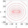
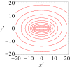
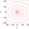
Figure 1: Logarithmically spaced contour plots of density in the three principal planes for a model with $v_{0}=1$, $q=0.9$ and $a=6$. Distances are given in units of $R_{\rm c}$.

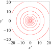
Figure 2: Logarithmically spaced contour plots of surface density for a model with $v_{0}=1$, $q=0.9$ and $a=6$. From left to right: $z^{\prime}=z$ (downwards-on), $z^{\prime}=y$ (edge-on), $z^{\prime}=x$ (face-on). Distances are given in units of $R_{\rm c}$.

2 The Logarithmic Bar Model

2.1 Potential-Density Pair

Long & Murali (1992) introduced the idea of weighting spherical or axisymmetric potentials with a needle-like density to give triaxial potentials. They explored barred models based on underlying Plummer (1911) or Miyamoto & Nagai (1975) potentials. Despite succeeding work by Vogt & Letelier (2010), the technique has remained largely unexplored. Here, we let the underlying potential be denoted by $\Phi_{\rm L}$ and be of logarithmic form

$$\Phi_{\rm L}(x,y,z)=\frac{v_{0}^{2}}{2}\ln(x^{2}+y^{2}+z^{2}q^{-2}+R_{\rm c}^{2}),$$ (3)

where $q$ is an axis ratio. This axisymmetric model has an asymptotically flat circular velocity curve of amplitude $v_{0}$. The properties of this model are discussed in Evans (1993) and Binney & Tremaine (2008).

The underlying potential $\Phi_{\rm L}$ is convolved with a thin “needle” density, $\lambda(x)$:

$$\Phi=\intop_{-\infty}^{\infty}\lambda(x^{\prime})\Phi_{\rm L}(x-x^{\prime},y,z)dx^{\prime}.$$ (4)

In this case, we choose $\lambda(x)$ to be a box function, spanning $[-a,a]$ and normalised such that $\intop_{-a}^{a}\lambda(x)dx=1$. The result is:

$$\Phi=\frac{v_{0}^{2}}{4a}\bigg{[}\chi\ln(\chi^{2}+T^{2})+2T\arctan\bigg{(}\frac{\chi}{T}\bigg{)}\bigg{]}_{x-a}^{x+a},$$ (5)

where $T=\sqrt{R_{\rm c}^{2}+y^{2}+z^{2}/q^{2}}$, and we have adopted the notation:

$$\bigg{[}f(\chi)\bigg{]}_{x_{1}}^{x_{2}}\equiv f(x_{2})-f(x_{1}),$$ (6)

which we shall use throughout the paper. This arises naturally because the operation used to obtain the potential is a definite integral. The corresponding density can then be obtained using Poisson’s equation:

$$\rho = \frac{v_{0}^{2}}{8\pi Gaq^{2}T^{2}}\bigg{[}\frac{(q^{2}R_{c}^{2}+(1-q^{-2})z^{2})\chi}{\chi^{2}+T^{2}}$$ (7)

$$\qquad\qquad+\frac{\big{(}(1+q^{2})R_{c}^{2}+y^{2}+z^{2}\big{)}\arctan\bigg{(}\dfrac{\chi}{T}\bigg{)}}{T}\bigg{]}_{x-a}^{x+a}.$$

We shall refer to this model as the logarithmic bar. The density represents the total self-gravitating matter, both luminous and dark. It is highly triaxial near the centre, but becomes axisymmetric at large radii. A necessary and sufficient condition for positive density is $q>1/\sqrt{2}$, just as for the logarithmic potential itself (see Binney & Tremaine 2008). Furthermore, if $R_{\rm c}=0$, then the density diverges along the $x$-axis, which is undesirable. For practical purposes, therefore, $R_{\rm c}>0$. Sample density contours are shown in Fig. 1, from which we can see that the model can attain highly triaxial and extended shapes. Within the bar regime, the density on the major axis falls typically by a factor of $\sim 2$ from the centre to the end of the bar ($|x|\sim a$). At large distances, the density falls off like

$$\rho(x,0,0)\sim{v_{0}^{2}\over 4\pi Gq^{2}x^{2}},\qquad\rho(0,0,z,)\sim{v_{0}^{2}(2-q^{-2})\over 4\pi Gz^{2}}.$$ (8)

We see that, far from the bar, the model looks like the axisymmetric logarithmic potential. To represent a barred galaxy, we keep in mind the picture that the inner parts are luminous, whilst the outer parts are dominated by dark matter which provides the flat rotation curve.

The gravitational forces are:

$$F_{x}= \quad-\bigg{[}\frac{v_{0}^{2}}{4a}\ln(\chi^{2}+T^{2})\bigg{]}_{x-a}^{x+a},$$

$$F_{y}= \quad-\bigg{[}\frac{v_{0}^{2}y}{2aT}\arctan\bigg{(}\frac{\chi}{T}\bigg{)}\bigg{]}_{x-a}^{x+a},$$ (9)

$$F_{z}= \quad-\bigg{[}\frac{v_{0}^{2}z}{2aq^{2}T}\arctan\bigg{(}\frac{\chi}{T}\bigg{)}\bigg{]}_{x-a}^{x+a}.$$

We have written this out explicitly to emphasise the fact that orbit integration in the model is very fast, as the force components contain only elementary functions.

The model contains four parameters: $v_{0}$, $a$, $R_{c}$ and $q$. The physical interpretations of these constants are as follows: $v_{0}$ remains the asymptotic rotation speed in the galactic plane, just as for the original logarithmic potential; $q$ is the axis ratio of the equipotentials in the $(y,z)$ plane (as well as the axis ratio at large distances from the origin in the $(x,z)$ plane); $a$ has the simple interpretation of being the half-length of the bar. Finally, the ratio $a/R_{c}$ is related to the axis ratios of the bar in the $(x,y)$ and $(x,z)$ planes, in the sense that a larger value of $a/R_{\rm c}$ corresponds to more extreme axis ratios. This degree of freedom may be removed, however, by working with $R_{\rm c}$ as the unit length: this will be the case for the remainder of this paper. In these units, $a$ both quantifies the half-length of the bar and the aforementioned axis ratios.

We remark that our four-parameter triaxial bar model compares very favourably with the competition! A triaxial Ferrers bar already has four free parameters, and it still has to be embedded in an axisymmetric background which normally has at least a further two or three (Teuben & Sanders, 1985; Kaufmann & Patsis, 2005). The bar models devised by Long & Murali (1992) also needed to be immersed in a background model for practical use (Hattori et al., 2016).

2.2 Equipotentials

Unlike the case of a Ferrers bar, the equipotentials of this model do not lie on similar concentric ellipsoids. Yet, an axis ratio is still a useful quantification of the geometry of the bar. If we Taylor expand the potential around the origin, we find:

$$\Phi=\frac{v_{0}^{2}}{2}\bigg{(}\frac{x^{2}}{a^{2}+1}+\frac{(y^{2}+z^{2}/q^{2})\arctan[a]}{a}\bigg{)}+\ldots$$ (10)

We can clearly see that, close to the centre, the equipotentials approximately lie on concentric ellipsoids, and hence meaningful axis ratios may be extracted. The $(y,z)$ axis ratio is simply $q$, but the $(x,y)$ axis ratio is less trivial.

A prescription for choosing a value of $a$ that approximately satisfies a given axis ratio in the $(x,y)$ plane, $p_{\Phi}$, is readily given as

$$a = \tan\theta,$$

$$\theta = \bigg{[}\frac{7}{2}-\frac{7^{2/3}3}{2\zeta}+\frac{7^{1/3}}{2}\zeta\bigg{]}^{1/2}$$ (11)

$$\zeta = \bigg{[}-11-45p_{\Phi}^{2}+\sqrt{5}\sqrt{62+198p_{\Phi}^{2}+405p_{\Phi}^{4}}\bigg{]}^{1/3}$$

The axis ratio is exactly $\sqrt{\mathrm{sinc}\,2\theta}$. This prescription is very effective, overestimating $p_{\Phi}$ by less than one per cent down to an axis ratio of $p_{\Phi}\simeq 0.5$, rising to approximately six per cent when $p_{\Phi}\simeq 0.3$.

The approach of Taylor expanding close to the origin is not effective in the case of the density, both because the expansion is more complicated than that of the potential, and because the density is more flattened than the potential in this region. Since the axis ratios of the density are of interest because they represent the physical dimensions of the bar itself, we suggest the following convention: we use the values on the $y$ and $z$ axes at which the density is equal to $\rho(a,0,0)$ to compute the axis ratios, since this is consistent with the physical interpretation of $a$ as the half-length of the bar. We note that this must be done numerically, and that the behaviour scales roughly as $p_{\rho}\sim(1+a)^{-1}$.

Model	$p_{\Phi}$	$p_{\rho}$	$a$	$\Omega_{b}$
Weak Bar	0.5	0.46	2.85	0.33
Strong Bar	0.3	0.14	7.55	0.13

Table 1: Parameters for the two models used. In both cases $v_{0}=1$.

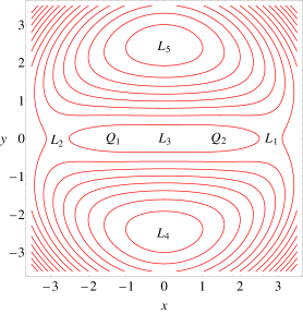
Figure 3: Contours of the effective potential for the weak bar model. $L_{4}$ and $L_{5}$ are maxima, $L_{1}$ and $L_{2}$ are saddle points, and $L_{3}$ is a minimum. If $\Omega_{b}>\Omega_{\rm crit}$, $L_{3}$ is a saddle point and the minima $Q_{1}$ and $Q_{2}$ appear.

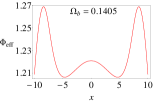
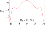
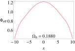
Figure 4: The evolution of the effective potential along the $x$-axis with $\Omega_{b}$ in the strong bar model, for which $\Omega_{\rm crit}=0.1313$. Notice the emergence of additional stationary points in the third panel.

2.3 Surface Density

To evaluate the surface density along a general line of sight, we must transform from internal coordinates ($x,y,z$) to projected coordinates ($x^{\prime},y^{\prime},z^{\prime}$). For a triaxial system, there are two viewing angles $\vartheta$ and $\varphi$. The required transformation is (see e.g., Evans et al., 2000):

$$\left(\begin{array}[]{c}x\\ y\\ z\end{array}\right)=\left(\begin{array}[]{ccc}-\sin\vartheta&-\cos\varphi\sin\vartheta&\cos\varphi\sin\vartheta\\ \cos\varphi&-\sin\varphi\cos\vartheta&\sin\varphi\sin\vartheta\\ 0&\sin\vartheta&\cos\vartheta\end{array}\right)\left(\begin{array}[]{c}x^{\prime}\\ y^{\prime}\\ z^{\prime}\end{array}\right).$$ (12)

For arbitrary viewing angles, the integration along the line of sight needs to be done numerically. However, when the line of sight coincides with one of the principal axes of the figure, the results are analytic.

This illustrates an advantage of this method of creating barred potentials. Any quantity that is computed using a linear operation on $\Phi$ can be first computed for the kernel (in this case $\Phi_{\rm L}$), and then convolved with the needle density. Hence, we can compute the surface densities for the barred model using the results from the axisymmetric model. We emphasise that the constraint $q>1/\sqrt{2}$ is necessary to ensure that the model is physical and has everywhere positive three dimensional density. Projecting along the $z^{\prime}=z$ axis gives (in units $R_{\rm c}=1$):

$$\Sigma(x^{\prime},y^{\prime})=\frac{qv_{0}^{2}}{8aG(1+y^{\prime 2})}\bigg{[}\frac{\chi}{P(\chi)}+(1+{y^{\prime}}^{2})\ln[\chi+P(\chi)]\bigg{]}_{x^{\prime}-a}^{x^{\prime}+a},$$ (13)

where $P(\chi)=\sqrt{1+\chi^{2}+y^{\prime 2}}$. Here, the barred galaxy is being viewed face-on.

Projecting along the $z^{\prime}=y$ axis gives:

$$\Sigma(x^{\prime},y^{\prime})=\frac{v_{0}^{2}}{8aGq^{2}(1+{y^{\prime}}^{2}/q^{2})}\bigg{[}\frac{\chi(q^{2}+(1-q^{-2}){y^{\prime}}^{2})}{Q(\chi)}$$

$$+(1+{y^{\prime}}^{2}/q^{2})\ln[\chi+Q(\chi)]\bigg{]}_{x^{\prime}-a}^{x^{\prime}+a},$$ (14)

where $Q(\chi)=\sqrt{1+\chi^{2}+{y^{\prime}}^{2}/q^{2}}$. This expression is useful when considering edge-on galaxies, which are a topic of much interest observationally. The surface density profile along the bar major axis is flattish. Typically, the surface density falls from its central value by a factor of $\lesssim 2$ by the end of the bar along the major axis ($|x^{\prime}|\sim a$). Along the minor axis at $|y^{\prime}|\sim a$, the fall-off factor is of course much steeper ($\sim 5$, depending on the choices of $q$ and $a$).

The final projection along a principal axis is $z^{\prime}=x$, which yields:

$$\Sigma(x^{\prime},y^{\prime})=\frac{v_{0}^{2}}{4Gq^{2}T^{3}}\Big{(}1+q^{2}+{x^{\prime}}^{2}+{y^{\prime}}^{2}\Big{)}.$$ (15)

Plots of the surface density are shown in Fig. 2 for the face-on, edge-on and downwards-on cases. Of course, this is the total (luminous and dark) surface density.

3 Orbital Structure

Here, we provide an analysis of the in-plane orbital structure (with figure rotation) of this potential. The planar periodic orbits that exist at various energies play a crucial role. They sire orbital families that librate around the periodic orbits. Ultimately, this information gives us insight into how the stars moving along these different orbits generate the density distribution, and hence the potential.

The Hamiltonian is:

$$H_{\rm J} = \frac{1}{2}(\dot{x}^{2}+\dot{y}^{2})+\Phi_{\rm eff}(x,y),$$ (16)

$$\Phi_{\rm eff}(x,y) = \Phi(x,y)-\frac{1}{2}\Omega_{b}^{2}(x^{2}+y^{2}),$$

where $\Omega_{\rm b}$ is the pattern speed and the phase space coordinates are written in terms of the frame in which the potential is static. The quantity $\Phi_{\rm eff}$ is known as the effective potential. The Hamiltonian is conserved in the rotating frame and is called the Jacobi constant (which we shall loosely refer to as the energy). The equations of motion are then extracted using Hamilton’s equations, and orbits are integrated numerically.

Note that the potential of the whole model is steady in a frame rotating with pattern speed $\Omega_{\rm b}$. So, the figure of the inner triaxial bar rotates. However, the outer parts are axisymmetric, and there is no difference between figure rotation and orbital streaming in axisymmetry. So, the orbital streaming (or the odd part of the distribution function) can be chosen so that there is no net rotation of the outer parts.

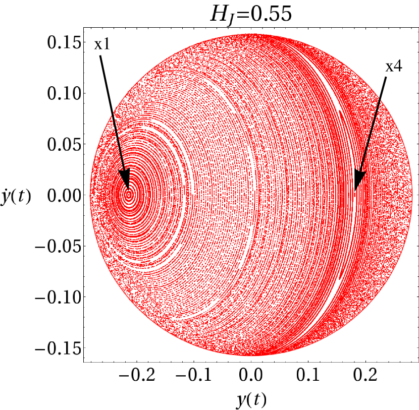
Figure 5: A surface of section for the weak bar model at Jacobi energy $H_{J}=0.55$. The location of the $x_{1}$ and $x_{4}$ periodic orbits are marked.

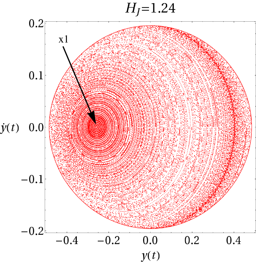
Figure 6: A typical surface of section for the strong bar model. At this energy ($H_{J}=1.24$), the $x_{1}$ periodic orbit and its family dominates. There are no stable $x_{4}$ orbits.

Figure 7: A surface of section of the strong bar model, but with $\Omega_{b}>\Omega_{\rm crit}$ ($\Omega_{b}=0.1405$), in the regime when $Q_{1}$ and $Q_{2}$ exist. The periodic orbits are two off-centered $x_{4}$ orbits that circulate around $Q_{1}$ and $Q_{2}$. There is a chaotic layer associated with the separatrix.

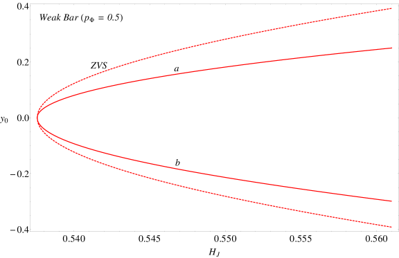
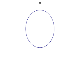
Figure 8: Characteristic diagram of stable orbits with multiplicity 1 for the weak bar model. This potential has a very simple orbital structure, with the retrograde $x_{4}$ ($a$) and prograde $x_{1}$ ($b$) orbits dominating.

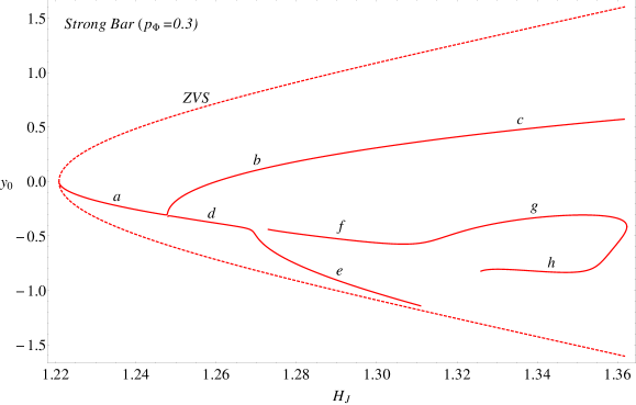
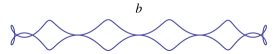
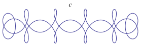
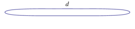
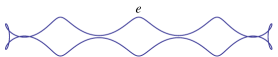
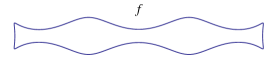
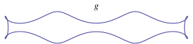
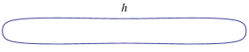
Figure 9: Characteristic diagram of stable orbits with multiplicity 1 for the strong bar model. Orbits belonging to the various families within the diagram are depicted below. Orbits with negative/positive $y_{0}$ are prograde/retrograde.

3.1 The Effective Potential

For most galaxies, the concensus is that corotation occurs at (or just beyond) the edge of the bar. This assertion is consistent with results from observations (Aguerri et al., 2003), orbital investigations (Patsis et al., 1997), and simulations (Pfenniger & Friedli, 1991; Athanassoula, 1992). In our model, the following prescription may be used to choose $\Omega_{\rm b}$ such that this requirement is satisfied:

$$\Omega_{\rm b}=\Omega_{0}(a)=\sqrt{\frac{-F_{x}(a,0)}{a}},$$ (17)

where $F_{x}(a,0)$ is the radial force at the end of the bar long axis. This gives the effective potential the usual structure, seen in Fig. 3, where L₁ to L₅ are the familiar Lagrange radii (see e.g., Binney & Tremaine 1987).

If the pattern speed is large enough, however, then the well-known morphology changes. There exists a critical pattern speed

$$\Omega_{\rm crit}(a)=\big{(}1+a^{2})^{-1/2},$$ (18)

such that if $\Omega_{\rm b}>\Omega_{\rm crit}$, the Lagrange point $L_{3}$ becomes a saddle point. In addition, two more minima then appear: $Q_{1}$ and $Q_{2}$. This effect goes unnoticed for bars where $a\lesssim 3$, since $\Omega_{\rm crit}(a)<\Omega_{0}(a)$ in this case. Fig. 4 depicts the various shapes the effective potential may take as $\Omega_{\rm b}$ is increased. In this regime, along the $x$-axis $L_{3}$ is a maximum and $Q_{1},Q_{2}$ are minima. Orbits can then become bound in the regions surrounding $Q_{1}$ and $Q_{2}$, creating overdensities. The existence of additional stationary points in the effective potential has been noticed before by Häfner et al. (2000) in a numerically constructed model of the Milky Way bar, though there the stationary points were off-axis. Multiple Lagrange may be common in bars with flattish profiles. The Freeman (1966a, b) bars, which have homogeneous density, may see their whole major axis as a Lagrange equilibrium line when the rotation frequency is equal to the long axis oscillation frequency. So, flattish bars, the central parts of which may be nearly homogeneous, may possesses multiple Lagrange points, the equilibirum line transforming to several points.

This feature may have observational consequences. It is well-known that many galactic bars exhibit a peanut morphology (Lütticke et al., 2000). This could be produced by stars librating around such additional on-axis Lagrange points like $Q_{1}$ and $Q_{2}$. In this picture, the peanut morphology may be interpreted as an effect related to the balance between centrifugal forces and self-gravity in a rotating strong bar.

3.2 Surfaces of Section and Characteristic Diagrams

A powerful tool for analysing orbital structure is the Poincaré surface of section. In a 2D potential, the phase space of a star has four coordinates, $(x,y,\dot{x},\dot{y})$, and cannot be visualised. However, one can see a depleted picture of this phase space by fixing the value of $H_{\rm J}$, and then plotting points when a given orbit intersects a chosen plane. These points are known as consequents, and the 2D plot is a surface of section.

In this analysis, we fix $H_{\rm J}$ and then plot the values of $(y,\dot{y})$ when an orbit upwardly intersects the $x=0$ plane ($\dot{x}>0$). We do this for a variety of initial conditions. Periodic orbits that upwardly intersect the $x$-axis with multiplicity $n$ appear in these diagrams as a set of $n$ invariant points, and quasiperiodic orbits form invariant curves around the invariant points (parent orbits). Chaotic orbits simply fill the phase-space available to them. The boundary of each surface of section is the zero velocity surface (ZVS) and is defined by the energy condition

$$\frac{1}{2}\dot{y}^{2}+\Phi_{\rm eff}(0,y)\leq\frac{1}{2}(\dot{x}^{2}+\dot{y}^{2})+\Phi_{\rm eff}(0,y)=H_{J}(x=0).$$ (19)

A characteristic diagram is a related concept to that of a surface of section. A family of periodic orbits will exist at a range of energies, and it is useful to monitor its evolution as well as possible bifurcations. We characterise a given family by the curve

$$y_{0}=f(H_{j}),$$ (20)

where $y_{0}$ is the $y$-coordinate at which the orbit upwardly intersects the $x$-axis (i.e. using the same convention as in the surfaces of section). A different curve of the form of eqn (20) exists for each family of periodic orbits. In practice, one is interested in the stable orbits of low multiplicity, since these will be the orbits that trap the most matter. Hence, in our characteristic diagrams, only orbits of multiplicity one are considered. In order to construct such a diagram, one needs to locate a periodic orbit using a surface of section, and then extrapolate to other energies by using suitable root-finding techniques (Contopoulos, 2002; Hasan et al., 1993).

3.3 Weak and Strong Logarithmic Bars

In order to understand the effects of bar strength, we provide results for two cases: a weak bar and strong bar. The parameters for each model are given in Table 1. We pick $\Omega_{\rm b}=\Omega_{0}(a)$ in the weak bar model, and $\Omega_{\rm b}=\Omega_{\rm crit}(a)$ in the strong bar model. For the strong bar case, this moves corotation to $x\simeq\pm 1.22a$.

The surfaces of section for the weak logarithmic bar all depict a very similar structure, which is shown in Fig 5. Indicated is the long-axis $x_{1}$ orbit (following the nomenclature in Contopoulos 2002), and the corresponding quasiperiodic orbits that are parented by it. These elongated orbits trap most of the stars in order to form the bar. The other noticeable resonance is the retrograde $x_{4}$ orbit, which will be far less populated than the $x_{1}$ orbits, since it is elongated along the short-axis of the bar. The surface of section is ruled by invariant curves and there are few chaotic orbits.

For comparison, Fig. 6 is a surface of section of the strong bar. At this energy ($H_{J}=1.24$), the $x_{4}$ family are unstable and have disappeared from the surface of section, so the orbital structure is dominated by $x_{1}$ orbits. As mentioned in Sect 3.1, if the pattern speed is large enough, two more minima ($Q_{1}$ and $Q_{2}$) appear in the effective potential. Orbits are indeed trapped around these minima, and this is demonstrated in Fig. 7. This surface of section is generated using $(x,\dot{x})$ as the phase-space coordinates and $y=0$, since off-centre orbits do not intersect the $y$-axis. Two ‘islands’ are visible, with parent orbits at their centres. These are off-centre $x_{4}$ orbits circulating around the extra Lagrangian points $Q_{1}$ and $Q_{2}$. Notice too that there is a clearly visible chaotic layer associated with the separatrix.

Figs 8 and 9 are the characteristic diagrams for the models considered here. The simple nature of the orbital structure of the weak bar is clear from its characteristic diagram, which exhibits no bifurcations or additional families whatsoever. However, the strong bar presents a different picture. As the energy increases, we see successive bifurcations from the $x_{1}$ sequence. These have an extended ’bow tie’ shape (see orbits f and g), albeit of more and more elaborate form. True $x_{1}$ orbits only exist in the very central parts of the model (below $H_{J}\approx 1.25$). With their extremely slender shape, these orbits look more like the propeller orbits identified by Kaufmann & Patsis (2005) in their study of a $n=2$ Ferrers bar embedded in a Plummer sphere. However, there are some differences. In the characteristic diagrams of Kaufmann & Patsis (2005), the $x_{1}$ orbits and propellers can coexist over some range of energies, with the propeller family eventually taking over (see their Figure 1). Here, the propeller orbits bifurcate from the $x_{1}$ sequence. This morphology in the characteristic diagram appears not to have been reported before, probably because previous investigations have often focussed on Ferrers bars. The logarithmic bar deviates very strongly from the elliptic density contours of Ferrers bars, so qualitatively new features in the characteristic diagram are to be expected.

We expect that these elongated and narrow orbits will trap most of the stars in the bar region in order to form the bar backbone. However, even in the case of the strong bar, this potential has a relatively simple orbital structure, with $x_{1}$ and then propeller orbits providing the dominant families.

4 Conclusions

The paper has introduced the logarithmic bar, which is elongated and triaxial in the central parts, but becomes axisymmetric at large radii. It is produced by convolving a needle density with the familiar logarithmic potential that generates a flat rotation curve  (Evans, 1993; Binney & Tremaine, 2008). Note that the entire model represents both the luminous and dark matter in a barred galaxy, as the model retains the appealing property of its progenitor in possessing an asymptotically flat rotation curve. Many of the properties of the model – the potential, the density, the force field and the surface density along the principal axes – are analytic. The surface density profile along the bar major axis is flattish, typically falling by factors of $\sim 2$ from centre to bar end. This is characteristic of bars in early-types (SB0, SBa), for which there is ample observational evidence for such flattish, slowly declining profiles (Elmegreen & Elmegreen, 1985; Sellwood & Wilkinson, 1993; Elmegreen et al., 1996).

Much of our insight into the orbital structure of bars is derived from studies of Ferrers and Freeman ellipsoids (see e.g., Contopoulos, 2002). These are analytically tractable, but are too homogeneous to represent real galactic bars. Unlike Ferrers bars, the density contours of the logarithmic bar are not ellipsoidal, but strongly elongated and spindly. The orbital structure of these new models is qualitatively different from Ferrers bars.

Weak logarithmic bars have a very simple orbital structure, with almost all stars moving on the retrograde $x_{4}$ and prograde $x_{1}$ orbits. As the bar strength and pattern speed are increased, additional stationary points of the effective potential can occur on the major axis. This phenomenon appears to be new, and it allows families of off-centered $x_{4}$ orbits to exist stably. This may have observational consequences, as it is a mechanism of maintaining long-lived peanut structures. Strong logarithmic bars also have a simple but unusual orbital make-up. At low energies, the $x_{1}$ orbital family still exists, although the $x_{4}$ family does not. However, at higher energies, propeller orbits (essentially very narrow $x_{1}$ orbits with superposed epicyclic oscillations) bifurcate from the $x_{1}$ sequence and take over. Their thinness enables extremely slender bars to be built. This provides a new family – in addition to the one reported by Kaufmann & Patsis (2005) – for which $x_{1}$ orbits are not the principal means of building the bar. The morphology of the characteristic diagrams is therefore different to any in the literature.

Our new model has many attractive features, both for fitting to barred spirals and for dynamical investigations. In particular, its simplicity compares favourably with its competitors. For example, Ferrers bars must always be supplemented by a spherical or axisymmetric background representing halo and disk to yield a cumbersome multi-component and multi-parameter galaxy.

Bars in late-type galaxies (SBb, SBc) are very different (Elmegreen et al., 1996). They have exponentially declining surface density profiles along the major axis, together with Gaussian cross-sections in the transverse directions. The versatile Long & Murali (1992) algorithm is capable of generating models with precisely these properties. A companion paper presents the properties of these exponential bars, which provide a fitting contrast to the flattish logarithmic bars studied here.

References

- Aguerri et al. (2003) Aguerri J. A. L., Debattista V. P., Corsini E. M., 2003, MNRAS, 338, 465
- Athanassoula (1992) Athanassoula E., 1992, MNRAS, 259, 328
- Athanassoula et al. (1983) Athanassoula E., Bienaymé O., Martinet L., Pfenniger D., 1983, AA, 127, 349
- Barbanis & Woltjer (1967) Barbanis B., Woltjer L., 1967, ApJ, 150, 461
- Binney & Tremaine (2008) Binney J., Tremaine S., 2008, Galactic Dynamics: Second Edition. Princeton University Press
- Contopoulos (1979) Contopoulos G., 1979, AA, 71, 221
- Contopoulos (1980) Contopoulos G., 1980, AA, 81, 198
- Contopoulos (2002) Contopoulos G., 2002, Order and Chaos in Dynamical Astronomy. Springer Verlag, Berlin
- de Vaucouleurs (1964) de Vaucouleurs G., 1964, Australian Academy of Sciences, Canberra, 195
- de Vaucouleurs & Freeman (1972) de Vaucouleurs G., Freeman K. C., 1972, 14, 163
- Dwek et al. (1995) Dwek E., Arendt R. G., Hauser M. G., Kelsall T., Lisse C. M., Moseley S. H., Silverberg R. F., Sodroski T. J., Weiland J. L., 1995, ApJ, 445, 716
- Elmegreen & Elmegreen (1985) Elmegreen B. G., Elmegreen D. M., 1985, ApJ, 288, 438
- Elmegreen et al. (1996) Elmegreen B. G., Elmegreen D. M., Chromey F. R., Hasselbacher D. A., Bissell B. A., 1996, \aj, 111, 2233
- Evans (1993) Evans N. W., 1993, MNRAS, 260, 191
- Evans et al. (2000) Evans N. W., Carollo C. M., de Zeeuw P. T., 2000, MNRAS, 318, 1131
- Ferrers (1877) Ferrers N. M., 1877, Quart. J. Pure and Applied Math, 14, 1
- Freeman (1966a) Freeman K. C., 1966a, MNRAS, 134, 1
- Freeman (1966b) Freeman K. C., 1966b, MNRAS, 134, 15
- Häfner et al. (2000) Häfner R., Evans N. W., Dehnen W., Binney J., 2000, MNRAS, 314, 433
- Hasan et al. (1993) Hasan H., Pfenniger D., Norman C., 1993, ApJ, 409, 91
- Hattori et al. (2016) Hattori K., Erkal D., Sanders J. L., 2016, MNRAS, 460, 497
- Kaufmann & Patsis (2005) Kaufmann D. E., Patsis P. A., 2005, ApJ, 624, 693
- Lindblad (1956) Lindblad B., 1956, Stockholms Observatoriums Annaler, 19, 2
- Long & Murali (1992) Long K., Murali C., 1992, ApJ, 397, 44
- Lütticke et al. (2000) Lütticke R., Dettmar R.-J., Pohlen M., 2000, \aaps, 145, 405
- Masters et al. (2011) Masters K. L., Nichol R. C., Hoyle B., Lintott C., Bamford S. P., Edmondson E. M., Fortson L., Keel W. C., Schawinski K., Smith A. M., Thomas D., 2011, MNRAS, 411, 2026
- Papayannopoulos & Petrou (1983) Papayannopoulos T., Petrou M., 1983, AA, 119, 21
- Patsis et al. (1997) Patsis P. A., Athanassoula E., Quillen A. C., 1997, ApJ, 483, 731
- Pfenniger (1984) Pfenniger D., 1984, AA, 134, 373
- Pfenniger & Friedli (1991) Pfenniger D., Friedli D., 1991, AA, 252, 75
- Sellwood & Wilkinson (1993) Sellwood J. A., Wilkinson A., 1993, Reports on Progress in Physics, 56, 173
- Teuben & Sanders (1985) Teuben P. J., Sanders R. H., 1985, MNRAS, 212, 257
- Vogt & Letelier (2010) Vogt D., Letelier P. S., 2010, MNRAS, 408, 1649