Classifying bent functions by their Cayley graphs

Abstract

In 1999 Bernasconi and Codenotti noted that the Cayley graph of a bent function is strongly regular. This paper describes the concept of extended Cayley equivalence of bent functions, discusses some connections between bent functions, designs, and codes, and explores the relationship between extended Cayley equivalence and extended affine equivalence. SageMath scripts and CoCalc worksheets are used to compute and display some of these relationships, for bent functions up to dimension 8.

1 Introduction

Binary bent functions are important combinatorial objects. Besides the well-known application of bent functions and their generalizations to cryptography [2] [65, 4.1-4.6], bent functions have well-studied connections to Hadamard difference sets [21], symmetric designs with the symmetric difference property [22, 33], projective two-weight codes [11, 23] and strongly regular graphs.

In two papers, Bernasconi and Codenotti [3], and then Bernasconi, Codenotti and Vanderkam [4] explored some of the connections between bent functions and strongly regular graphs. While these papers established that the Cayley graph of a binary bent function (whose value at 0 is 0) is a strongly regular graph with certain parameters, they leave open the question of which strongly regular graphs with these parameters are so obtained.

In a recent paper [44], the author found an example of two infinite series of bent functions whose Cayley graphs have the same strongly regular parameters at each dimension, but are not isomorphic if the dimension is 8 or more.

Kantor, in 1983 [34], showed that the numbers of non-isomorphic projective linear two weight codes with certain parameters, Hadamard difference sets, and symmetric designs with certain properties, grow at least exponentially with dimension. This result suggests that the number of strongly regular graphs obtained as Cayley graphs of bent functions also increases at least exponentially with dimension.

A 2003 paper by Cameron [12] considers random strongly regular graphs with given parameters, and outlines some prerequisites for a theory of random strongly regular graphs, including that “the number of non-isomorphic graphs is superexponential in the number of vertices.”

The goal of the current paper is to further explore the connections between bent functions, their Cayley graphs, and related combinatorial objects, and in particular to examine the relationship between various equivalence classes of bent functions, in particular, the relationship between the extended affine equivalence classes and equivalence classes defined by isomorphism of Cayley graphs. As well as a theoretical study of bent functions of all dimensions, a computational study is conducted into bent functions of dimension at most 8, using SageMath [63] and CoCalc [58].

The methodology for this study is modelled on experimental mathematics. As stated by Borwein and Devlin [5, pp. 4-5]:

What makes experimental mathematics different (as an enterprise) from the classical conception and practice of mathematics is that the experimental process is regarded not as a precursor to a proof, to be relegated to private notebooks and perhaps studied for historical purposes only after a proof has been obtained. Rather, experimentation is viewed as a significant part of mathematics in its own right, to be published, considered by others, and (of particular importance) contributing to our overall mathematical knowledge.

The theoretical results listed this paper serve a few purposes. First, in order to classify bent functions by their Cayley graphs, it helps to understand the relationship between Cayley equivalence and other concepts of equivalence of bent functions, especially if this helps to cut down the search space needed for the classification. A similar consideration applies to the duals of bent functions. Second, some of the empirical observations made in the classification of bent functions in small dimensions can be explained by these theoretical results. Third, these theoretical results can improve our understanding of the relationships between bent functions, projective two-weight codes, strongly regular graphs, and symmetric block designs with the symmetric difference property. In what follows, known results with references are presented as propositions, or sometimes as remarks; and results where the statement or the proof seems to be missing or obscure within the existing literature are presented as lemmas or theorems, with proofs.

This paper makes no pretence at being an exhaustive survey, neither should it be construed that the lemmas and theorems listed here make any claim to originality. Even given the current excellent electronic search capabilities available, it would be folly to do so given the extensive literature that has been generated on the study of bent functions since the 1960s. Some recent surveys include books by Cusick and Stanica [19], Mesnager [50] and Tokareva [65], and the article by Carlet and Mesnager [16].

The remainder of the paper is organized as follows. Section 2 covers the concepts, definitions and known results used later in the paper. Section 3 discusses the relationship between bent functions and strongly regular graphs. Section 4 introduces various concepts of equivalence of bent functions. Section 5 discusses the relationship between bent functions and block designs. Section 6 describes the SageMath and CoCalc code that has been used to obtain the computational results of this paper. Section 7 puts the results of this paper in the context of questions that are still open. The appendices contain the proof of one of the properties of quadratic bent functions, and list some of the properties of the equivalence classes of bent functions for dimension up to 8.

2 Preliminaries

This section presents some of the key concepts used in the remainder of the paper. We first examine Boolean functions, then define bent Boolean functions, and finally explore the relationships between bent functions and Hamming weights.

2.1 Boolean functions

Here and in the remainder of the paper, $\mathbb{F}_{2}$ denotes the field of two elements, also known as $GF(2)$. Models of $\mathbb{F}_{2}$ include integer arithmetic modulo 2 ($\mathbb{Z}/2\mathbb{Z}$ also known as $\mathbb{Z}_{2}$) and Boolean algebra with “exclusive or” as addition and “and” as multiplication.

Boolean functions and Reed-Muller codes.

Any Boolean function $f:\mathbb{F}_{2}^{n}\rightarrow\mathbb{F}_{2}$ can be represented as a reduced polynomial in at most $n$ variables over $F_{2}$ [51, 55] [21, Ch. III, Section 2]. This is called the algebraic normal form of $f$ [57, Chapter 5].

Example.

In Sage, using sage.crypto.boolean_function, define:

       
       from sage.crypto.boolean_function import BooleanFunction
       f = BooleanFunction([1,1,1,0])
       a = f.algebraic_normal_form()

The algebraic normal form of the Boolean function f on $\mathbb{F}_{2}^{2}$ with variables $x_{0}$ and $x_{1}$ and truth table $\immediate\NoHyper\ref{@sageinline0}$ (in lexicographic order) is then a = $\immediate\NoHyper\ref{@sageinline1}$ [64, Boolean Functions].

Definition 1.

[51] [45, Ch. 13, Section 3] [62, 10.5.2] The Reed-Muller code $RM(r,n)$ consists of those Boolean functions $f:\mathbb{F}_{2}^{n}\rightarrow\mathbb{F}_{2}$ whose algebraic normal form has degree $r$.

Remark.

Some texts use the notation $\mathcal{R}(r,n)$ or $RM(r,2^{n})$ for $RM(r,n)$.

Each Reed-Muller code $RM(r,n)$ is a linear subspace of the vector space of Boolean functions $f:\mathbb{F}_{2}^{n}\rightarrow\mathbb{F}_{2}$.

The Reed-Muller code $RM(1,n)$ consists of the $2^{n+1}$ affine functions $f(x)=\langle c,x\rangle+\delta$ for $c\in\mathbb{F}_{2}^{n},\ \delta\in\mathbb{F}_{2}$ [45, Ch 14, Section 3] [62, 10.5.2].

Bent Boolean functions.

Bent Boolean functions can be defined in a number of equivalent ways. The definition used here involves the Walsh Hadamard Transform.

Definition 2.

[21, Ch. III, Section 2] [45, Ch. 2, Section 3] The Walsh Hadamard transform of a Boolean function $f:\mathbb{F}_{2}^{n}\rightarrow\mathbb{F}_{2}$ is

$$W_{f}(x) :=\sum_{y\in\mathbb{F}_{2}^{n}}(-1)^{f(y)+\langle x,y\rangle}$$

where

$$\langle x,y\rangle :=\sum_{i=0}^{n-1}x_{i}y_{i}.$$

Example.

Using sage.crypto.boolean_function in Sage, define:

       
       from sage.crypto.boolean_function import BooleanFunction
       f = BooleanFunction([1,1,1,0])
       w = f.walsh_hadamard_transform()

The Walsh Hadamard transform of the Boolean function f on $\mathbb{F}_{2}^{2}$ is then w = $\immediate\NoHyper\ref{@sageinline2}$ as a truth table in lexicographic order [64, Boolean Functions].

Remarks.

1. In versions of Sage before 8.2 the walsh_hadamard_transform method has an incorrect sign [Sage trac ticket #23931].

2. For Boolean functions $f:\mathbb{F}_{2^{n}}\rightarrow\mathbb{F}_{2}$, where $\mathbb{F}_{2^{n}}$ is the finite field on $2^{n}$ elements, the trace form [29, 3.1]

   is used to define the Walsh Hadamard transform.

Definition 3.

A Boolean function $f:\mathbb{F}_{2}^{2m}\rightarrow\mathbb{F}_{2}$ is bent if and only if its Walsh Hadamard transform has constant absolute value $2^{m}$ [21, p. 74] [55, p. 300].

Example.

The Boolean function f in the previous example is bent, since its Walsh Hadamard transform has constant absolute value $\immediate\NoHyper\ref{@sageinline3}$.

The remainder of this paper refers to bent Boolean functions simply as bent functions.

Remarks.

1. Bent functions can also be characterized as those Boolean functions whose Hamming distance from any affine Boolean function is the maximum possible [45, Ch. 14 Theorem 6] [49, Theorem 3.3].

2. The property of being a bent function is invariant with respect to the non-degenerate symmetric bilinear form used to define the Walsh Hadamard transform. That is, for a non-degenerate symmetric bilinear form $\langle x,Sy\rangle$, where $S$ is a non-degenerate symmetric matrix in $\mathbb{F}_{2}^{n\times n}$, and a Boolean function $f:\mathbb{F}_{2^{n}}\rightarrow\mathbb{F}_{2}$, the Walsh Hadamard transform

   $$W[S]_{f}(x) :=\sum_{y\in\mathbb{F}_{2}^{n}}(-1)^{f(y)+\langle x,Sy\rangle}$$

   has constant absolute value $2^{m}$ if and only if $f$ is bent as per Definition 3 [24]. In this sense, given an isomorphism between $\mathbb{F}_{2}^{2m}$ and $\mathbb{F}_{2^{2m}}$ as vector spaces over $\mathbb{F}_{2}$, the definition of a bent function on $\mathbb{F}_{2}^{2m}$ is equivalent to the definition on $\mathbb{F}_{2^{2m}}$.

3. The fact that any symmetric matrix $S$ on $\mathbb{F}_{2}^{n}$ can be factorized $S=L^{T}L$, with the shape of $L$ depending on the rank of $S$ [39] leads to the existence of a basis of $\mathbb{F}_{2^{n}}$ for which the trace form is diagonal. This yields an explicit isomorphism between $\mathbb{F}_{2}^{2m}$ and $\mathbb{F}_{2^{2m}}$ as vector spaces over $\mathbb{F}_{2}$ for which the two equivalent definitions of bent function coincide [53, p. 860].

The characterization of bent functions given by Definition 3 immediately implies the existence of dual functions:

Definition 4.

For a bent function $f:\mathbb{F}_{2}^{2m}\rightarrow\mathbb{F}_{2}$, the function $\widetilde{f}$, defined by

$$(-1)^{\widetilde{f}(x)} :=2^{-m}W_{f}(x)$$

is called the dual of $f$ [15].

Remark 1.

The function $\widetilde{f}$ is also a bent function on $\mathbb{F}_{2}^{2m}$ [45, p. 427] [55, p. 301].

2.2 Weights and weight classes

Definition 5.

The Hamming weight of a Boolean function is the cardinality of its support [45, p. 8]. For $f$ on $\mathbb{F}_{2}^{n}$

$$\operatorname{supp}\left(f\right) :=\{x\in\mathbb{F}_{2}^{n}\mid f(x)=1\},\quad\operatorname{wt}\left(f\right):=\left|\operatorname{supp}\left(f\right)\right|.$$

The remainder of this paper refers to Hamming weights simply as weights.

Since a bent function of a given dimension can have only one of two weights, the weights can be used to define equivalence classes of bent functions here called weight classes.

Definition 6.

A bent function $f$ on $\mathbb{F}_{2}^{2m}$ has weight [21, Theorem 6.2.10]

$$\operatorname{wt}\left(f\right) =2^{2m-1}-2^{m-1}\quad(\text{weight class number~{}}\operatorname{wc}\left(f\right)=0),\text{~{}or}$$

$$\operatorname{wt}\left(f\right) =2^{2m-1}+2^{m-1}\quad(\text{weight class number~{}}\operatorname{wc}\left(f\right)=1).$$

Weight classes and dual bent functions.

We now note a connection between weight classes and dual bent functions that makes it a little easier to reason about dual bent functions. The following lemma expresses the dual bent function in terms of weight classes. (See also MacWilliams and Sloane [45, p. 414].)

Lemma 1.

For a bent function $f:\mathbb{F}_{2}^{2m}\rightarrow\mathbb{F}_{2}$, and $x\in\mathbb{F}_{2}^{2m}$,

$$\widetilde{f}(x) =\operatorname{wc}\left(y\mapsto f(y)+\langle x,y\rangle\right).$$

The proof of Lemma 1 relies on the following lemma about weight classes.

Lemma 2.

For a bent function $f:\mathbb{F}_{2}^{2m}\rightarrow\mathbb{F}_{2}$,

$$\operatorname{wc}\left(f\right) =2^{-m}\operatorname{wt}\left(f\right)-2^{m-1}+2^{-1},$$

so that

$$\operatorname{wt}\left(f\right) =2^{m}\operatorname{wc}\left(f\right)+2^{2m-1}-2^{m-1}.$$

Proof.

If $\operatorname{wt}\left(f\right)=2^{2m-1}-2^{m-1}$ then

$$2^{-m}\operatorname{wt}\left(f\right)-2^{m-1}+2^{-1} =2^{-m}(2^{2m-1}-2^{m-1})-2^{m-1}+2^{-1}=0.$$

If $\operatorname{wt}\left(f\right)=2^{2m-1}+2^{m-1}$ then

$$2^{-m}\operatorname{wt}\left(f\right)-2^{m-1}+2^{-1} =2^{-m}(2^{2m-1}+2^{m-1})-2^{m-1}+2^{-1}=1.$$

∎

Proof of Lemma 1. Let $h(y):=y\mapsto f(y)+\langle x,y\rangle.$ Then

$$(-1)^{\widetilde{f}(x)} =2^{-m}\sum_{y\in\mathbb{F}_{2}^{2m}}(-1)^{f(y)+\langle x,y\rangle}$$

$$=2^{-m}\left(\sum_{f(y)+\langle x,y\rangle=0}1-\sum_{f(y)+\langle x,y\rangle=1}1\right)$$

$$=2^{-m}\left(2^{2m}-2\operatorname{wt}\left(h\right)\right)=2^{m}-2^{1-m}\operatorname{wt}\left(h\right)$$

$$=2^{m}-2^{1-m}(2^{m}\operatorname{wc}\left(h\right)+2^{2m-1}-2^{m-1})$$

$$=1-2\operatorname{wc}\left(h\right)=(-1)^{\operatorname{wc}\left(h\right)},$$

where we have used Lemma 2. ∎

3 Bent functions and strongly regular graphs

This section defines the Cayley graph of a Boolean function, and explores the relationships between bent functions, projective two-weight codes, and strongly regular graphs.

3.1 The Cayley graph of a Bent function

The Cayley graph of a bent function $f$ with $f(0)=0$ is defined in terms of the Cayley graph for a general Boolean function with $f$ with $f(0)=0$.

The Cayley graph of a Boolean function.

Definition 7.

For a Boolean function $f:\mathbb{F}_{2}^{2m}\rightarrow\mathbb{F}_{2}$, with $f(0)=0$ we consider the simple undirected Cayley graph $\operatorname{Cay}\left(f\right)$ [3, 3.1] where the vertex set $V(\operatorname{Cay}\left(f\right))=\mathbb{F}_{2}^{2m}$ and for $i,j\in\mathbb{F}_{2}^{2m}$, the edge $(i,j)$ is in the edge set $E(\operatorname{Cay}\left(f\right))$ if and only if $f(i+j)=1$.

Note especially that in contrast with the paper of Bernasconi and Codenotti [3], this paper defines Cayley graphs only for Boolean functions $f$ with $f(0)=0$, since the use of Definition 7 with a function $f$ for which $f(0)=1$ would result in a graph with loops rather than a simple graph.

Bent functions and strongly regular graphs.

We repeat below in Proposition 1 the result of Bernasconi and Codenotti [3] that the Cayley graph of a bent function is strongly regular. The following definition is used to fix the notation used in this paper.

Definition 8.

A simple graph $\Gamma$ of order $v$ is strongly regular [6, 9, 59] with parameters $(v,k,\lambda,\mu)$ if

• each vertex has degree $k,$

• each adjacent pair of vertices has $\lambda$ common neighbours, and

• each nonadjacent pair of vertices has $\mu$ common neighbours.

The following proposition summarizes some of the well-known properties of the Cayley graphs of bent functions.

Proposition 1.

The Cayley graph $\operatorname{Cay}\left(f\right)$ of a bent function $f$ on $\mathbb{F}_{2}^{2m}$ with $f(0)=0$ is a strongly regular graph with $\lambda=\mu$ [3, Lemma 12].

In addition, any Boolean function $f$ on $\mathbb{F}_{2}^{2m}$ with $f(0)=0$, whose Cayley graph $\operatorname{Cay}\left(f\right)$ is a strongly regular graph with $\lambda=\mu$ is a bent function [4, Theorem 3] [61, Theorem 3.1].

For a bent function $f$ on $\mathbb{F}_{2}^{2m}$, the parameters of $\operatorname{Cay}\left(f\right)$ as a strongly regular graph are [21, Theorem 6.2.10] [28, Theorem 3.2]

$$(v,k,\lambda,\mu)= (4^{m},2^{2m-1}-2^{m-1},2^{2m-2}-2^{m-1},2^{2m-2}-2^{m-1})$$

or $$(4^{m},2^{2m-1}+2^{m-1},2^{2m-2}+2^{m-1},2^{2m-2}+2^{m-1}).$$

3.2 Bent functions, linear codes and strongly regular graphs

Another well known way to obtain a strongly regular graph from a bent function is via a projective two-weight code. This is done via the following definitions.

Projective two-weight binary codes.

Definition 9.

[7, 11, 20, 23, 66]

A two-weight binary code with parameters $[n,k,d]$ is a $k$ dimensional subspace of $\mathbb{F}_{2}^{n}$ with minimum Hamming distance $d$, such that the set of Hamming weights of the non-zero vectors has size 2.

Bouyukliev, Fack, Willems and Winne [7, p. 60] define projective codes as follows. “A generator matrix $G$ of a linear code $[n,k]$ code $C$ is any matrix of rank $k$ (over $\mathbb{F}_{2}$) with rows from $C.$ …A linear $[n,k]$ code is called projective if no two columns of a generator matrix $G$ are linearly dependent, i.e., if the columns of $G$ are pairwise different points in a projective $(k-1)$-dimensional space.”

A projective two-weight binary code with parameters $[n,k,d]$ is thus a two-weight binary code with these parameters which is also projective as an $[n,k]$ linear code.

Remark 2.

In the case of $\mathbb{F}_{2}$, no two columns of the generator matrix of a projective code are equal.

From bent function to strongly regular graph via a projective two-weight code.

There is a standard construction for obtaining a projective two-weight code from a bent function in such a way that the code can be used to define a strongly regular graph. This method is equivalent to the following definition.

Definition 10.

[23]. See also [11, Definition 2A]

Let $v=2^{2m}$, and let $X$ be the matrix in $\mathbb{F}_{2}^{2m\times v}$ whose columns are the $v$ elements of $\mathbb{F}_{2}^{2m}$ in lexicographic order. For a Boolean function $f:\mathbb{F}_{2}^{2m}\rightarrow\mathbb{F}_{2}$, let $n=\operatorname{wt}\left(f\right)$, and let $Y$ be the matrix in $\mathbb{F}_{2}^{2m\times n}$ whose columns are the $n$ elements of $\operatorname{supp}\left(f\right)$ in lexicographic order. That is,

$$Y_{i,j} =(y_{j})_{i},\quad\text{for~{}}i\in\{0,\ldots,v-1\},\ j\in\{0,\ldots,n-1\},$$

with $y_{j}\in\mathbb{F}_{2}^{2m}$ being an element of $\operatorname{supp}\left(f\right)$.

The linear code $C(f)\subset\mathbb{F}_{2}^{n}$ is then given by the span of the $2m$ rows of $Y$ within $\mathbb{F}_{2}^{n}$, considered as row vectors.

Example.

In Sage, using sage.crypto.boolean_function and
boolean_cayley_graphs.boolean_linear_code, define:

       
       from sage.crypto.boolean_function import BooleanFunction
       from boolean_cayley_graphs.boolean_linear_code import (
            boolean_linear_code)
       f = BooleanFunction([0,1,0,0,0,1,0,0,1,0,0,0,0,0,1,1])
       dim = f.nvariables()
       Cf = boolean_linear_code(dim, f)

The linear code $Cf:=C(f)$ of the Boolean function f on $\mathbb{F}_{2}^{4}$ then has the following generator matrix in echelon form:

$$\immediate\NoHyper\ref{@sageinline4}.$$

[42] [64, Boolean Functions].

Remarks.

1. The linear span of the rows of $Y$ is given by the set of rows of the matrix

   $$M :=X^{T}Y,\quad\text{where}$$

   $$X \in\mathbb{F}_{2}^{2m\times v}$$

   is the matrix whose columns are all $v$ elements of $\mathbb{F}_{2}^{2m}$ in lexicographic order. Thus $M\in\mathbb{F}_{2}^{v\times n}$.

2. Definition 10 is not identical to the generic construction described by Ding [23, Section III] since that definition is for subsets $D\subset\mathbb{F}_{v}$, and uses the trace form, but for the case where $D$ is the support of a Boolean function $f\colon\mathbb{F}_{v}\rightarrow F_{2}$, the two definitions are equivalent.

   If the bilinear form $\langle x,y\rangle=x^{T}y$ is replaced in the previous remark by a non-degenerate symmetric bilinear form $\langle x,Sy\rangle=x^{T}Sy$, where $S$ is a non-degenerate symmetric matrix in $\mathbb{F}_{2}^{2m\times 2m}$, then this would produce the same linear code, since the matrix $S$, being invertible, produces a bijection on $\mathbb{F}_{2}^{2m}$ and therefore the matrix $X^{T}S$ differs from $X^{T}$ only by a permutation of rows.

   Thus by similar arguments to those in Remarks 2 and 3 following Definition 3, the generic construction described by Ding [23, Section III] is in this case equivalent to Definition 10.

When $f$ is a bent function, the linear code $C(f)$ described by Definition 10 has the following properties.

Proposition 2.

[23, Corollary 10]

For a bent function $f:\mathbb{F}_{2}^{2m}\rightarrow\mathbb{F}_{2}$, the linear code $C(f)$ is a projective two-weight binary code, with

$$\begin{cases}n=\operatorname{wt}\left(f\right)=2^{2m-2}-2^{m-2},\quad k=2m&\text{if~{}}\operatorname{wc}\left(f\right)=0.\\ n=\operatorname{wt}\left(f\right)=2^{2m-2}+2^{m-2},\quad k=2m&\text{if~{}}\operatorname{wc}\left(f\right)=1.\end{cases}$$

The possible weights of non-zero code words are:

$$\begin{cases}2^{2m-2},2^{2m-2}-2^{m-1}&\text{if~{}}\operatorname{wc}\left(f\right)=0.\\ 2^{2m-2},2^{2m-2}+2^{m-1}&\text{if~{}}\operatorname{wc}\left(f\right)=1.\end{cases}$$

Proof.

We examine $W_{f}$, the Walsh Hadamard transform of $f$.

$$W_{f}(x) =\sum_{y\in\mathbb{F}_{2}^{2m}}(-1)^{\langle x,y\rangle+f(y)}=\sum_{y\in\mathbb{F}_{2}^{2m}}(-1)^{\langle x,y\rangle}-2\sum_{f(y)=1}(-1)^{\langle x,y\rangle}.$$

But

$$\sum_{y\in\mathbb{F}_{2}^{2m}}(-1)^{\langle x,y\rangle} =\begin{cases}4^{m}&(x=0)\\ 0&\text{otherwise},\end{cases}$$

as per the Sylvester Hadamard matrices.

So, for $x\neq 0$,

$$W_{f}(x) =-2\sum_{f(y)=1}(-1)^{\langle x,y\rangle},$$

so

$$\sum_{f(y)=1}(-1)^{\langle x,y\rangle} =\operatorname{wt}\left(f\right)-2\sum_{\begin{subarray}{c}f(y)=1\\ \langle x,y\rangle=1\end{subarray}}1=-W_{f}(x)/2.$$

But

$$\sum_{\begin{subarray}{c}f(y)=1\\ \langle x,y\rangle=1\end{subarray}}1 =\operatorname{wt}\left(x^{T}Y\right),$$

the weight of the code word of $C(f)$ corresponding to $x$. So

$$\operatorname{wt}\left(f\right)-2\operatorname{wt}\left(x^{T}Y\right) =-W_{f}(x)/2,$$

and therefore

$$\operatorname{wt}\left(x^{T}Y\right) =\operatorname{wt}\left(f\right)/2+W_{f}(x)/4.$$

We now examine the two possible weight class numbers of $f$.

If $\operatorname{wc}\left(f\right)=0$ then $\operatorname{wt}\left(f\right)=2^{2m-1}-2^{m-1}$. For $x\neq 0$ there are two cases, depending on $\widetilde{f}(x)$:

If $\widetilde{f}(x)=0$ then $W_{f}(x)=2^{m}$, so

$$\operatorname{wt}\left(x^{T}Y\right) =2^{2m-2}-2^{m-2}+2^{m-2}=2^{2m-2}.$$

If $\widetilde{f}(x)=1$ then $W_{f}(x)=-2^{m}$, so

$$\operatorname{wt}\left(x^{T}Y\right) =2^{2m-2}-2^{m-2}-2^{m-2}=2^{2m-2}-2^{m-1}.$$

Similarly, if $\operatorname{wc}\left(f\right)=1$ then $\operatorname{wt}\left(f\right)=2^{2m-1}+2^{m-1}$, and so for $x\neq 0$

$$\operatorname{wt}\left(x^{T}Y\right) =\begin{cases}2^{2m-2}+2^{m-1}&(\widetilde{f}(x)=0)\\ 2^{2m-2}&(\widetilde{f}(x)=1).\end{cases}$$

As a consequence, all $v=2^{2m}$ rows of $M=X^{T}Y$ are distinct, since the rows of $M$ consist of every linear combination of the rows of $Y$, every linear combination of the rows of $Y$ is given by some $x^{T}Y$ where $x$ is a column of $X$, and for every non-zero $x$, this linear combination has positive weight and is therefore non-zero. Thus the dimension of $C(f)$ as a subspace of $F_{2}^{n}$ is $k=2m$. ∎

From linear code to strongly regular graph.

This paper uses the following non-standard definition to obtain a strongly regular graph from a projective two-weight code.

Definition 11.

Given $f:\mathbb{F}_{2}^{2m}\rightarrow\mathbb{F}_{2}$, and linear code $C(f)$ defined as per Definition 10, define the graph $R(f)$ as follows.

Vertices of $R(f)$ are code words of $C(f)$.

For code words $v,w\in C(f)$, edge $(u,v)\in R(f)$ if and only if

$$\begin{cases}\operatorname{wt}\left(u+v\right)=2^{2m-2}-2^{m-1}&(\text{if~{}}\operatorname{wc}\left(f\right)=0).\\ \operatorname{wt}\left(u+v\right)=2^{2m-2}+2^{m-1}&(\text{if~{}}\operatorname{wc}\left(f\right)=1).\end{cases}$$

Remarks.

1. The standard definition uses the lower of the two weights in both cases above.

2. Since $C(f)$ is a projective two-weight binary code, $R(f)$ is a strongly regular graph [20, Theorem 2] [13, Theorem 16.22].

The graph $R(f)$ is the Cayley graph of the extended dual.

The strongly regular graph $R(f)$ of bent function $f$, as per 11 has the following remarkable property.

Theorem 1.

For a bent function $f:\mathbb{F}_{2}^{2m}\rightarrow\mathbb{F}_{2}$, with $f(0)=0$,

$$R(f)\equiv\operatorname{Cay}\left(\widetilde{f}+\operatorname{wc}\left(f\right)\right).$$

Proof.

As a consequence of Lemma 1, $\operatorname{wc}\left(f\right)=\widetilde{f}(0)$, so if $g(x):=\widetilde{f}(x)+\operatorname{wc}\left(f\right)$ then $g(0)=0$ and therefore the Cayley graph of $g$ is well defined.

From the proof of Proposition 2:

If $\operatorname{wc}\left(f\right)=0$ then for $x\neq 0$

$$\operatorname{wt}\left(x^{T}Y\right) =\begin{cases}2^{2m-2}&(\widetilde{f}(x)=0)\\ 2^{2m-2}-2^{m-1}&(\widetilde{f}(x)=1).\end{cases}$$

Thus for $x\neq 0$, if $\widetilde{f}(x)+\operatorname{wc}\left(f\right)=1$ if and only if $\operatorname{wt}\left(x^{T}Y\right)=2^{2m-2}-2^{m-1}$.

If $\operatorname{wc}\left(f\right)=1$ then for $x\neq 0$

$$\operatorname{wt}\left(x^{T}Y\right) =\begin{cases}2^{2m-2}+2^{m-1}&(\widetilde{f}(x)=0)\\ 2^{2m-2}&(\widetilde{f}(x)=1).\end{cases}$$

Thus for $x\neq 0$, if $\widetilde{f}(x)+\operatorname{wc}\left(f\right)=1$ if and only if $\operatorname{wt}\left(x^{T}Y\right)=2^{2m-2}+2^{m-1}$.

Thus in both cases, $R(f)$ as per Definition 11 is isomorphic to the Cayley graph $\operatorname{Cay}\left(\widetilde{f}+\operatorname{wc}\left(f\right)\right)$. ∎

4 Equivalence of bent functions

The following concepts of equivalence of Boolean functions are used in this paper, usually in the case where the Boolean functions are bent.

Extended affine equivalence.

Definition 12.

For Boolean functions $f,g:\mathbb{F}_{2}^{n}\rightarrow\mathbb{F}_{2}$, $f$ is extended affine equivalent to $g$ [65, Section 1.4] if and only if

$$g(x) =f(Ax+b)+\langle c,x\rangle+\delta$$

for some $A\in GL(n,2)$, $b,c\in\mathbb{F}_{2}^{n}$, $\delta\in\mathbb{F}_{2}$.

The Boolean function $f$ is extended affine equivalent to $g$ if and only if $f$ and $g$ are in the same orbit of the action of the extended general affine group $EGA(n,2)$ on $\mathbb{F}_{2}^{\mathbb{F}_{2}^{n}}$, defined as follows.

Definition 13.

$$EGA(n,2):=\{(A,b,c,\delta)\mid A\in GL(n,2),\ b,c\in\mathbb{F}_{2}^{n},\ \delta\in\mathbb{F}_{2}\}$$

with

$$(A,b,c,\delta)(A^{\prime},b^{\prime},c^{\prime},\delta^{\prime}):=(AA^{\prime},Ab^{\prime}+b,A^{\prime T}c+c^{\prime},\langle c,b^{\prime}\rangle+\delta+\delta^{\prime}),$$

with action

$$(A,b,c,\delta)f(x) :=f(Ax+b)+\langle c,x\rangle+\delta,$$

$$\left((A,b,c,\delta)(A^{\prime},b^{\prime},c^{\prime},\delta^{\prime})f\right) :=(A^{\prime},b^{\prime},c^{\prime},\delta^{\prime})\circ(A,b,c,\delta)f$$

$$=(A^{\prime},b^{\prime},c^{\prime},\delta^{\prime})\left((A,b,c,\delta)f\right).$$

[46, Section 2]

Proposition 3.

The extended affine (EA) equivalence classes of the Boolean functions $\mathbb{F}_{2}^{n}\rightarrow\mathbb{F}_{2}$, that is, the orbits of these functions under $EGA(n,2)$, have the following well known and easily verified properties.

1. For a given $f\colon\mathbb{F}_{2}^{n}\rightarrow\mathbb{F}_{2}$, the $2^{n+1}$ functions $x\mapsto f(x)+\langle c,x\rangle+\delta$ are all distinct. Thus the EA equivalence class of $f$ consists of some number of complete cosets of the Reed-Muller code $RM(1,n)$ described in Section 2.1.

2. Each general affine transformation $(A,b)f(x):=f(Ax+b)$ preserves cosets of the Reed-Muller code $RM(1,n)$ in the sense that $(A,b)$ maps $f+RM(1,n)$ to $g+RM(1,n)$ where $g(x)=f(Ax+b)$.

See also MacWilliams and Sloane [45, Ch. 13], and Maiorana [46].

General linear equivalence.

Definition 14.

For Boolean functions $f,g:\mathbb{F}_{2}^{n}\rightarrow\mathbb{F}_{2}$, $f$ is general linear equivalent to $g$ if and only if

$$g(x) =f(Ax)$$

for some $A\in GL(n,2)$.

Thus $f$ is general linear equivalent to $g$ if and only if $f$ and $g$ are in the same orbit of the action of the general linear group $GL(n,2)$ on $\mathbb{F}_{2}^{\mathbb{F}_{2}^{n}}$, defined as follows.

Definition 15.

$$Af(x) :=f(Ax),$$

$$(AA^{\prime})f :=A^{\prime}\circ Af=A^{\prime}(Af).$$

Some references for the study of the general linear equivalence of Boolean functions include Harrison [26], Comerford [18], and Maiorana [46, Section 2].

Extended translation equivalence.

Definition 16.

For Boolean functions $f,g:\mathbb{F}_{2}^{n}\rightarrow\mathbb{F}_{2}$, $f$ is extended translation equivalent to $g$ if and only if

$$g(x) =f(x+b)+\langle c,x\rangle+\delta$$

for $b,c\in\mathbb{F}_{2}^{n}$, $\delta\in\mathbb{F}_{2}$.

Thus $f$ is extended translation equivalent to $g$ if and only if $f$ and $g$ are in the same orbit of the action of the extended translation group $ET(n,2)$ on $\mathbb{F}_{2}^{\mathbb{F}_{2}^{n}}$, defined as follows.

Definition 17.

$$ET(n,2):=\{(b,c,\delta)\mid\ b,c\in\mathbb{F}_{2}^{n},\ \delta\in\mathbb{F}_{2}\}$$

with

$$(b,c,\delta)(b^{\prime},c^{\prime},\delta^{\prime}):=(b^{\prime}+b,c+c^{\prime},\langle c,b^{\prime}\rangle+\delta+\delta^{\prime}),$$

with action

$$(b,c,\delta)f(x) :=f(x+b)+\langle c,x\rangle+\delta,$$

$$\left((b,c,\delta)(b^{\prime},c^{\prime},\delta^{\prime})\right)f :=(b^{\prime},c^{\prime},\delta^{\prime})\circ(b,c,\delta)f$$

$$=(b^{\prime},c^{\prime},\delta^{\prime})\left((b,c,\delta)f\right).$$

Cayley equivalence.

Definition 18.

For Boolean functions $f,g:\mathbb{F}_{2}^{n}\rightarrow\mathbb{F}_{2}$, with $f(0)=g(0)=0$, we call $f$ and $g$ Cayley equivalent, and write $f\equiv g$, if and only if the graphs $\operatorname{Cay}\left(f\right)$ and $\operatorname{Cay}\left(g\right)$ are isomorphic.

Equivalently, $f\equiv g$ if and only if there exists a bijection $\pi:\mathbb{F}_{2}^{n}\rightarrow\mathbb{F}_{2}^{n}$ such that

$$g(x+y) =f\big{(}\pi(x)+\pi(y)\big{)}\quad\text{for all~{}}x,y\in\mathbb{F}_{2}^{n}.$$

Remark: Note that the bijection $\pi$ is not necessarily linear on $\mathbb{F}_{2}^{n}$. Examples of bent functions $f$ and $g$ where $f\equiv g$ but the bijection is not linear are given in Section B.

Extended Cayley equivalence.

While Bernasconi and Codenotti [3] define Cayley graphs for Boolean functions with $f(0)=1$ and allow Cayley graphs to have loops, this paper defines Cayley graphs only for Boolean functions where $f(0)=0$. This has the disadvantage that Cayley equivalence is an equivalence relation on half of the Boolean functions rather than all of them. To extend this equivalence relation to all Boolean functions, we just declare the functions $f$ and $f+1$ to be “extended” Cayley equivalent, resulting in the following definition.

Definition 19.

For Boolean functions $f,g:\mathbb{F}_{2}^{n}\rightarrow\mathbb{F}_{2}$, if there exist $\delta,\epsilon\in\{0,1\}$ such that $f+\delta\equiv g+\epsilon$, we call $f$ and $g$ extended Cayley (EC) equivalent and write $f\cong g$.

Extended Cayley equivalence is thus an equivalence relation on the set of all Boolean functions on $\mathbb{F}_{2}^{n}$. It is easy to verify that $f\cong g$ if and only if $f+f(0)\equiv g+g(0)$.

4.1 Relationships between different concepts of equivalence

As stated in the Introduction, in order to classify bent functions by their Cayley graphs, it helps to understand the relationship between Cayley equivalence and other concepts of equivalence of Boolean functions, especially if this helps to cut down the search space needed for the classification. This section lists a few of these useful relationships.

General linear equivalence implies Cayley equivalence.

Firstly, general linear equivalence of Boolean functions implies Cayley equivalence. Specifically, the following result applies.

Theorem 2.

If $f$ is a Boolean function with $f(0)=0$ and $g(x):=f(Ax)$ where $A\in GL(n,2)$, then $f\equiv g$.

Proof.

$$g(x+y) =f\big{(}A(x+y)\big{)}=f(Ax+Ay)\quad\text{for all~{}}x,y\in\mathbb{F}_{2}^{n}.$$

∎

Thus, for bent functions, the following result holds.

Corollary 3.

If $f$ is bent with $f(0)=0$ and $g(x):=f(Ax)$ where $A\in GL(n,2)$, then $g$ is bent with $g(0)=0$ and $f\equiv g$.

Thus if $f$ is bent with $f(0)=0$, and $g$ is bent with $g(0)=0$, and $f\not\equiv g$, then $f$ is not general linear equivalent to $g$. This result immediately leads to another corollary. Here, and later in this paper, we make use of the following terminology.

Definition 20.

A Boolean function $f\colon\mathbb{F}_{2}^{n}\rightarrow\mathbb{F}_{2}$ is said to be prolific if there is no pair $b,c\in\mathbb{F}_{2}^{n}$ with $g(x)=f(x+b)+\langle c,x\rangle+f(b)$ such that $f\cong g$. Thus the number of extended Cayley classes in the extended translation class of a prolific Boolean function is $4^{n}$.

Corollary 4.

If $f\colon\mathbb{F}^{2m}\rightarrow\mathbb{F}_{2}$ is bent with $f(0)=0$, and $f$ is prolific, then there is no triple $A\in GL(2m,2)$, $b,c\in\mathbb{F}_{2}^{2m}$ with $f(Ax)=f(x+b)+\langle c,x\rangle+f(b)$.

Extended affine, translation, and Cayley equivalence.

Secondly, if $f$ is a Boolean function, and $h$ is a Boolean function $h$ that is extended affine equivalent to $f$, then a Boolean function $g$ exists that is general linear equivalent to $h$ and extended translation equivalent to $f$:

Theorem 3.

For $A\in GL(n,2)$, $b,c\in\mathbb{F}_{2}^{n}$, $\delta\in\mathbb{F}_{2}$, $f:\mathbb{F}_{2}^{n}\rightarrow\mathbb{F}_{2}$, the function

$$h(x) :=f(Ax+b)+\langle c,x\rangle+\delta$$

can be expressed as $$h(x)=g(Ax)$$ where

$$g(x) :=f(x+b)+\langle(A^{-1})^{T}c,x\rangle+\delta.$$

Proof.

Let $y:=Ax$. Then

$$g(Ax)=g(y) =f(y+b)+\langle(A^{-1})^{T}c,y\rangle+\delta$$

$$=f(y+b)+\langle c,A^{-1}y\rangle+\delta$$

$$=f(Ax+b)+\langle c,x\rangle+\delta=h(x).$$

∎

Corollary 5.

If $f$ is a bent Boolean function, and a bent function $h$ is extended affine equivalent to $f$, then a bent function $g$ can be found that is extended Cayley equivalent to $h$ and extended translation equivalent to $f$.

Proof.

Let $f$, $g$, and $h$ be as per Theorem 3. If $f$ is bent, then so are $g$ and $h$. Since, by Theorem 3, $g$ is general linear equivalent to $h$, by Theorem 2, $g$ is extended Cayley equivalent to $h$. ∎

As a consequence, to determine which strongly regular graphs occur, corresponding to each extended Cayley equivalence classes within the extended affine equivalence class of a bent function $f:\mathbb{F}_{2}^{2m}\rightarrow\mathbb{F}_{2}$ with $f(0)=0$, we need only examine the extended translation equivalent functions of the form

$$f(x+b)+\langle c,x\rangle+f(b),$$

for each $b,c\in\mathbb{F}_{2}^{2m}$. This cuts down the required search space considerably.

Quadratic bent functions have only two extended Cayley classes.

Finally, in the case of quadratic bent functions, there is a complete classification in terms of weight classes.

Theorem 4.

For each $m>0$, the extended affine equivalence class of quadratic bent functions $q:\mathbb{F}_{2}^{2m}\rightarrow\mathbb{F}_{2}$ contains exactly two extended Cayley equivalence classes, corresponding to the two possible weight classes of $x\mapsto q(x+b)+\langle c,x\rangle+q(b)$.

The proof of this theorem is given in Appendix A.

4.2 Relationships between duality of bent functions and different concepts of equivalence

The following propositions are based on well known results, but are useful in understanding the relationship between the duality of bent functions and various concepts of equivalence.

Firstly, general linear equivalence of bent functions $f$ and $g$ implies general linear equivalence of their duals, $\widetilde{f}$ and $\widetilde{g}$, which implies Cayley equivalence of $\widetilde{f}$ and $\widetilde{g}$.

Proposition 4.

[21, Remark 6.2.7]

For a bent function $f:\mathbb{F}_{2}^{2m}\rightarrow\mathbb{F}_{2}$, and $A\in GL(2m,2)$, if

$$g(x) :=f(Ax)$$

then

$$\widetilde{g}(x) =\widetilde{f}\big{(}(A^{T})^{-1}x\big{)},$$

and therefore by Theorem 2, $\widetilde{g}\equiv\widetilde{f}$.

If, in addition, $f=\widetilde{f}$ then $\widetilde{g}\equiv g$.

Remark: Functions of the form

$$f(x):=\sum_{k=0}^{m-1}x_{2k}x_{2k+1}$$

are self dual bent functions, $f=\widetilde{f}$ [21, Remark 6.3.2]. There are many other self dual bent functions [15, 25].

Secondly, the following proposition displays a relationship between the extended translation class of a bent function $f$, and that of its dual $\widetilde{f}$.

Proposition 5.

[21, Remark 6.2.7] [14, Proposition 8.7].

For a bent function $f$ on $\mathbb{F}_{2}^{2m}$, and $b,c\in\mathbb{F}_{2}^{2m}$, if

$$g(x) :=f(x+b)+\langle c,x\rangle$$

then

$$\widetilde{g}(x) =\widetilde{f}(x+c)+\langle b,x\rangle+\langle b,c\rangle.$$

This result has an implication for the relationship between the set of bent functions within an extended translation (ET) equivalence class, and the set of their duals. Recall that a bent function is not necessarily extended affine (EA) equivalent to its dual [38]. The following “all or nothing” property holds within an extended translation equivalence class of bent functions.

Corollary 6.

For bent functions $f,g$ on $\mathbb{F}_{2}^{2m}$, if $f$ is EA equivalent to $\widetilde{f}$ and $g$ is ET equivalent to $f$, then $\widetilde{g}$ is EA equivalent to $g$. Thus, by Corollary 5, the set of isomorphism classes of Cayley graphs of the duals of the bent functions in the ET class of $f$ equals the set of isomorphism classes of Cayley graphs of the bent functions themselves.

Conversely, for a bent function $f$ on $\mathbb{F}_{2}^{2m}$, if there is any bent function $g$ that is ET equivalent to $f$, such that $\widetilde{g}$ is not EA equivalent to $g$, then no bent function in the ET class is EA equivalent to its dual, including $f$ itself.

5 Bent functions and block designs

This section examines the relationships between bent functions and symmetric block designs.

5.1 The two block designs of a bent function

The first block design of a bent function $f$ on $\mathbb{F}_{2}^{2m}$ is obtained by interpreting the adjacency matrix of $\operatorname{Cay}\left(f\right)$ as the incidence matrix of a block design. In this case we do not need $f(0)=0$ [22, p. 160].

The second block design of a bent function $f$ involves the symmetric difference property, which was first investigated by Kantor [33, Section 5].

Definition 21.

[33, p. 49].

A symmetric block design $\mathcal{D}$ has the symmetric difference property (SDP) if, for any three blocks, $B,C,D$ of $\mathcal{D},$ the symmetric difference $B\bigtriangleup C\bigtriangleup D$ is either a block or the complement of a block.

This second block design is defined as follows.

Definition 22.

For a bent function $f$ on $\mathbb{F}_{2}^{2m}$, define the matrix $M_{D}(f)\in\mathbb{F}_{2}^{2^{2m}\times 2^{2m}}$ where

$$M_{D}(f)_{c,x} :=f(x)+\langle c,x\rangle+\widetilde{f}(c),$$ (1)

and use it as the incidence matrix of a symmetric block design, which we call it the SDP design of $f$.

Kantor describes the special case where $f$ is quadratic [33, Section 5], and Dillon and Schatz [22] describe the general case. See also Cameron and van Lint [13, pp. 77-78 and Ex. 13, p. 152].

The following properties of SDP designs of bent functions are well known.

Proposition 6.

[22, p. 160] [52, Theorem 3.29]

For any bent function $f$ on $\mathbb{F}_{2}^{2m}$, the SDP design of $f$ has the symmetric difference property.

Proposition 7.

[22, p. 161] [34]

For bent functions $f,g$ on $\mathbb{F}_{2}^{2m}$, the two SDP designs $D(f)$ and $D(g)$ are isomorphic as symmetric block designs if and only if $f$ and $g$ are affine equivalent.

Weight classes and the SDP design matrix.

Definition 22 is different from but equivalent to the one given by Dillon and Schatz [22, p. 160]:

Lemma 7.

[52, 3.29]

For any bent function $f$ on $\mathbb{F}_{2}^{2m}$, the rows of the incidence matrix $M_{D}(f)$ are given by the words of minimum weight in the code spanned by the support of $f$ and the Reed-Muller code $RM(1,2m)$.

(Here we have used an ordering of the elements of $\mathbb{F}_{2}^{2m}$ to define an ordering of the columns of the incidence matrix.)

Proof.

Firstly, as mentioned in Section 2.1, the Reed-Muller code $RM(1,2m)$ consists of the words spanned by the affine functions on $Z_{2}^{2m}$. Thus, the incidence matrix $M_{RM(1,2m)}$ is defined by

$${M_{RM(1,2m)}}_{c,x} :=\langle c,x\rangle+d,$$

where $d\in\mathbb{F}_{2}$.

Therefore the incidence matrix of the code spanned by the support of $f$ and $RM(1,2m)$ is defined by

$${M_{f,RM(1,2m)}}_{c,x} :=f(x)+\langle c,x\rangle+d.$$

Finally, from Lemma 1 we know that

$$\operatorname{wc}\left(x\mapsto f(x)+\langle c,x\rangle\right) =\widetilde{f}(c),$$

so that

$$\operatorname{wc}\left(x\mapsto f(x)+\langle c,x\rangle+\widetilde{f}(c)\right) =0.$$

∎

The following characterization of the SDP design of a bent function $f$ also relies on Lemma 1 for its proof. We first define the matrix of weight classes corresponding to the extended translation class of $f$.

Definition 23.

For a bent function $f:\mathbb{F}_{2}^{2m}\rightarrow\mathbb{F}_{2}$, define the weight class matrix of $f$ by

$$M_{wc}(f)_{c,b} :=\operatorname{wc}\left(x\mapsto f(x+b)+\langle c,x\rangle+f(b)\right)$$

for $b,c\in\mathbb{F}_{2}^{2m}$.

Theorem 5.

The weight class matrix of $f$ as given by Definition 23 equals the incidence matrix of the SDP design of $f$. Specifically,

$$M_{wc}(f)_{c,b} =f(b)+\langle c,b\rangle+\widetilde{f}(c)$$

$$=M_{D}(f)_{c,b},$$

where $M_{D}(f)$ is defined by (1).

Proof.

Let $g(x):=f(x+b)+\langle c,x\rangle+f(b)$. Then by change of variable $y:=x+b$,

$$\operatorname{wc}\left(g\right) =\operatorname{wc}\left(y\mapsto f(y)+\langle c,y\rangle+\langle c,b\rangle+f(b)\right)$$

$$=\operatorname{wc}\left(y\mapsto f(y)+\langle c,y\rangle\right)+\langle c,b\rangle+f(b)$$

$$=\widetilde{f}(c)+\langle c,b\rangle+f(b),$$

as a consequence of Lemma 1. ∎

6 SageMath and CoCalc code

The computational results listed in this paper were obtained by the use of code written in Sage [30] [63] and Python. This code base is called Boolean-Cayley-graphs and it is available both as a GitHub repository [42] and as a public CoCalc [58] folder [43]. For an introduction to other aspects of coding theory and cryptography in Sage, see the article by Joyner et al. [30].

Description of the Sage code.

This section contains a brief description of some of the code included in Boolean-Cayley-graphs. More detailed documentation is being developed and this is intended to be included as part of the code base. The code itself is subject to review and revision, and may change as a result of the advice of those more experienced with Sage code. The description in this section applies to the code base as it exists in 2018.

The code base is structured as a set of Sage script files. These in turn use Python scripts, found in a subdirectory called Boolean_Cayley_graphs. The Python code is used to define a number of useful Python classes.

The key class is BentFunctionCayleyGraphClassification. This class is used to store the classification of Cayley graphs within the extended translation class of a given bent function $f$, as well as the classification of Cayley graphs of the duals of each function in the extended translation class. The class therefore contains the algebraic normal form of the given bent function, a list of graphs stored as strings obtained via the graph6_string [47] method of the Graph class, and two matrices, used to store the list indices corresponding to the Cayley graph for each bent function in the extended translation class, and the dual of each bent function, respectively. The class also contains the weight class matrix corresponding to the given bent function.

The class is initialized by enumerating the bent functions of the form $x\mapsto f(x+b)+\langle c,x\rangle+f(b)$, and determining the Cayley graph of each. For each Cayley graph, the Graph method canonical_label is used to invoke the Bliss package [31, 32] to calculate the canonical label of the graph, and then graph6_string is used to obtain a string. Each new graph is compared for isomorphism to each of the graphs in the current list, by simply comparing the string against each of the existing strings. If the new graph is not isomorphic to any existing graph, it is added to the list. Each list of pairwise non-isomorphic graphs can be checked by a function called check_graph_class_list which uses the Nauty package to check the non-isomorphism [47, 48].

It is the efficiency of the Bliss canonical labelling algorithm, and the speed of its implementation, that makes this approach feasible. Even so, for an 8 dimensional bent function, the initialization of its Cayley graph classification can take more than 24 hours on an Intel®Core™i7 CPU 870 running at 2.93 GHz. For this reason, each computed classification is saved, and a class method (load_mangled) is provided to load existing saved classifications.

History of the Sage code.

The Sage code originated in 2015 as a series of worksheets on SageMathCloud (now CoCalc). While these were useful for investigating extended Cayley classes for bent functions in up to 6 dimensions, they were too slow to use for bent functions in 8 dimensions.

The Boolean-Cayley-graphs GitHub project [42] and public SageMathCloud folder [43] were begun in 2016 with the intention of refactoring the code to make it fast enough to use for bent functions in 8 dimensions up to degree 3. The use of canonical labelling made this possible.

Further improvements were made in 2017 to enable the classification of any bent function in 8 dimensions or less to be computed in a reasonable time on a commodity personal computer. In late 2017, code was added so that the Cayley graph classifications could be accessed via a relational database [40], with implementations using SQLite3 [60] and PostgreSQL [54]. Also, parallel versions of the classification functions were written using MPI4Py, and used on the NCI Raijin supercomputer to complete the classifications for CAST-128 and compute the classifications of the $\mathcal{PS}^{(+)}$ bent functions in 8 dimensions. In 2018, the code was continually improved, and computation of the classifications of the $\mathcal{PS}^{(-)}$ bent functions in 8 dimensions was begun.

7 Discussion

The investigation of the extended Cayley classes of bent functions is just beginning, and there are many open questions.

The following questions have been settled only for dimensions 2, 4 and 6.

1. How many extended Cayley classes are there for each dimension? Are there “Exponential numbers” of classes [34]?

2. In $n$ dimensions, which extended translation classes contain the maximum number, $4^{n}$, of different extended Cayley classes?

3. Which extended Cayley classes overlap more than one extended translation class?

4. Which bent functions are Cayley equivalent to their dual?

In 8 dimensions, what are the extended affine and extended Cayley classes of bent functions of degree 4 [37]? What are the key properties of the strongly regular graphs obtained as Cayley graphs of bent functions, e.g., what is the distribution of clique numbers, clique polynomials, etc.? How do these distributions vary with the type of bent function, e.g., how do the distributions for the $\mathcal{PS}^{(-)}$ and $\mathcal{PS}^{(+)}$ partial spread bent functions differ from each other and from the general case?

Finally, how does the concept of extended Cayley classes of bent functions generalize to bent functions over number fields of prime order $p\neq 2$ [17]?

Acknowledgements.

This work was begun in 2014 while the author was a Visiting Fellow at the Australian National University, continued while the author was a Visiting Fellow and a Casual Academic at the University of Newcastle, Australia, and concluded while the author was an Honorary Fellow at the University of Melbourne, and an employee of the Bureau of Meteorology.

Thanks to Christine Leopardi for her hospitality at Long Beach. Thanks to Robert Craigen, Joanne Hall, Kathy Horadam, David Joyner, Philippe Langevin, William Martin, Padraig Ó Catháin, Judy-anne Osborn, Dima Pasechnik and William Stein for valuable questions, discussions and advice; David Joyner and Caroline Melles for suggestions for improvements based on the first draft of this paper; Nathan Clisby, for the opportunity to become an Honorary Fellow at the University of Melbourne; Kodlu, a member of MathOverflow, for asking Philippe Langevin about the affine classification of bent functions of degree 4 in 8 dimensions; Gray Chan for a citation tool for IETF RFCs; and finally, thanks to the authors of SageMath, Bliss, and Nauty for these valuable tools without which I would not have been able to conduct this research.

Appendix A Proof of Theorem 4

The proof of Theorem 4 relies on a number of supporting lemmas, which are stated and proved here.

Lemma 8.

Let $q(x):=x^{T}Lx$ where $L\in\mathbb{F}_{2}^{2m\times 2m}$,

$$L :=\left[\begin{array}[]{cc}0&I\\ 0&0\end{array}\right],$$

so that

$$q(x) =\sum_{k=0}^{m-1}x_{k}x_{m+k}.$$

Let $f(x):=q(x+b)+\langle c,x\rangle+q(b)$. Then there exists $c^{\prime}\in\mathbb{F}_{2}^{2m}$ such that

$$f(x) =q(x)+\langle c^{\prime},x\rangle.$$

Proof.

$$q(x)=x^{T}Lx,\quad\text{so~{}}q(x+b) =(x^{T}+b^{T})L(x+b)$$

$$=q(x)+x^{T}Lb+b^{T}Lx+q(b)$$

$$=q(x)+\langle(L+L^{T})b,x\rangle+q(b),$$

and therefore

$$q(x+b)+\langle c,x\rangle+q(b) =q(x)+\langle(L+L^{T})b+c,x\rangle.$$

∎

Lemma 9.

Let $Z\in\mathbb{F}_{2}^{2m\times 2m}$ be symmetric with zero diagonal. In other words, $Z=Z^{T}$, $\operatorname{diag}\left(Z\right)=0$. Then for any $M\in\mathbb{F}_{2}^{2m\times 2m}$,

$$x^{T}(M+Z)x =x^{T}Mx$$

for all $x\in\mathbb{F}_{2}^{2m}$.

Proof.

Let $Z$, $x$ be as above. Then

$$x^{T}Zx =\sum_{i=0}^{2m-1}\sum_{j=0}^{2m-1}x_{i}Z_{i,j}x_{j}$$

$$=\sum_{i=0}^{2m-1}\sum_{j<i}x_{i}Z_{i,j}x_{j}\,+\sum_{i=0}^{2m-1}x_{i}Z_{i,i}x_{i}\,+\sum_{i=0}^{2m-1}\sum_{j>i}x_{i}Z_{i,j}x_{j}$$

$$=\sum_{i=0}^{2m-1}\sum_{j<i}x_{i}(Z_{i,j}+Z_{j,i})=0.$$

Therefore

$$x^{T}(M+Z)x =x^{T}Mx+x^{T}Zx=x^{T}Mx.$$

∎

Lemma 10.

Let $q$ be defined as per Lemma 8. Then for all $c\in Z_{2}^{2m}$ with $q(c)=0$, there exists $A\in GL(2m,2)$ such that

$$q(Ax) =q(x)+\langle c,x\rangle.$$

Proof.

Let $C\in\mathbb{F}_{2}^{2m\times 2m}$ be such that $C_{i,j}=\delta_{i,j}c_{i}$, where $\delta$ is the Dirac delta: $\delta_{i,j}=1$ if $i=j$ and $0$ otherwise. In other words $\operatorname{diag}\left(C\right)=c$. Then

$$\langle c,x\rangle =\sum_{i=0}^{2m-1}c_{i}x_{i}$$

$$=\sum_{i=0}^{2m-1}x_{i}c_{i}x_{i}=x^{T}Cx.$$

Therefore, by Lemma 9,

$$q(x)+\langle c,x\rangle =x^{T}(L+Z+C)x,$$

where $Z\in\mathbb{F}_{2}^{2m\times 2m}$ is symmetric with zero diagonal.

For such $Z$, let $S:=Z+C$. We want to find $A\in\mathbb{F}_{2}^{2m\times 2m}$ such that $q(Ax)=q(x)+\langle c,x\rangle.$ In other words,

$$q(Ax) =(Ax)^{T}L(Ax)=x^{T}A^{T}LAx=x^{T}(L+S)x.$$

This will be true if $A^{T}LA=L+S.$

Let

$$A :=\left[\begin{array}[]{cc}A_{0,0}&A_{0,1}\\ A_{1,0}&A_{1,1}\end{array}\right],\quad S :=\left[\begin{array}[]{cc}S_{0,0}&S_{0,1}\\ S_{0,1}^{T}&S_{1,1}\end{array}\right]=:\left[\begin{array}[]{cc}Z_{0,0}+C_{0,0}&Z_{0,1}\\ Z_{0,1}^{T}&Z_{1,1}+C_{1,1}\end{array}\right].$$

Since

$$LA =\left[\begin{array}[]{cc}0&I\\ 0&0\end{array}\right]\left[\begin{array}[]{cc}A_{0,0}&A_{0,1}\\ A_{1,0}&A_{1,1}\end{array}\right]=\left[\begin{array}[]{cc}A_{1,0}&A_{1,1}\\ 0&0\end{array}\right],$$

we require that

$$A^{T}LA =\left[\begin{array}[]{cc}A_{0,0}&A_{1,0}\\ A_{0,1}&A_{1,1}\end{array}\right]\left[\begin{array}[]{cc}A_{1,0}&A_{1,1}\\ 0&0\end{array}\right]$$

$$=\left[\begin{array}[]{cc}A_{0,0}^{T}A_{1,0}&A_{0,0}^{T}A_{1,1}\\ A_{0,1}^{T}A_{1,0}&A_{0,1}^{T}A_{1,1}\end{array}\right]$$

$$=L+S=\left[\begin{array}[]{cc}S_{0,0}&I+S_{0,1}\\ S_{0,1}^{T}&S_{1,1}\end{array}\right],$$

and therefore

$$A_{0,0}^{T}A_{1,0} =S_{0,0},\quad A_{0,0}^{T}A_{1,1}=I+S_{0,1},$$

$$A_{0,1}^{T}A_{1,0} =S_{0,1}^{T},\quad A_{0,1}^{T}A_{1,1}=S_{1,1}.$$

If $S_{0,1}=0$ and $A_{0,0}=I$ then $A_{1,0}=S_{0,0}$, $A_{1,1}=I$ and $A_{0,1}=S_{1,1}$. In this case, we have $A_{0,1}^{T}A_{1,0}=S_{0,1}^{T}=0$, i.e. $S_{1,1}S_{0,0}=0$, and

$$A =\left[\begin{array}[]{cc}I&S_{1,1}\\ S_{0,0}&I\end{array}\right],$$

so that

$$A^{T}LA =\left[\begin{array}[]{cc}I&S_{0,0}\\ S_{1,1}&I\end{array}\right]\left[\begin{array}[]{cc}S_{0,0}&I\\ 0&0\end{array}\right]$$

$$=\left[\begin{array}[]{cc}S_{0,0}&I\\ 0&S_{1,1}\end{array}\right]$$

$$=L+S.$$

Also

$$S =\left[\begin{array}[]{cc}Z_{0,0}+C_{0,0}&0\\ 0&Z_{1,1}+C_{1,1}\end{array}\right].$$

Since $q(c)=0$ we have

$$q(c) =\sum_{k=0}^{m-1}c_{k}c_{m+k}=0.$$

Let $K:=\{k\mid c_{k}c_{m+k}=1\}$. Then we must have $\left|K\right|=2r$ for some integer $r\geqslant 0$, i.e. $\left|K\right|$ is even. We therefore arbitrarily group the elements of $K$ into pairs $(i_{p},j_{p})$ for $p=0,\ldots,r-1$, and define the matrix $T\in\mathbb{F}_{2}^{m\times m}$ by

$$T_{i,j} :=\sum_{p=0}^{r-1}(\delta_{i,i_{p}}\delta_{j,j_{p}}+\delta_{i,j_{p}}\delta_{j,i_{p}}),$$

so that

$$\begin{cases}T_{i_{p},j_{p}}=T_{j_{p},i_{p}}=1&\text{for~{}}p\in\{0,\ldots,r-1\},\\ T_{i,j}=0&\text{otherwise.}\end{cases}$$

Since the $r$ pairs $(i_{p},j_{p})$ partition the set $K$, the matrix $T$ has at most one non-zero in each row and column.

Recalling that

$$(T^{2})_{i,j} =\sum_{k=0}^{m-1}T_{i,k}T_{k,j},$$

we see that the general term $T_{i,k}T_{k,j}$ of this sum is non-zero only if either

$$\begin{cases}i=j=i_{p},&\text{and}\ k=j_{p},\ \text{or}\\ i=j=j_{p},&\text{and}\ k=i_{p},\end{cases}$$

for some $p\in\{0,\ldots,r-1\}$, with all $2r$ of these cases being mutually exclusive. So $T^{2}$ is diagonal with $2r$ non-zeros at the elements of $K$.

But $C_{1,1}C_{0,0}$ is diagonal, and $(C_{1,1}C_{0,0})_{i,i}=c_{m+i}c_{i}$. Therefore

$$T^{2} =C_{1,1}C_{0,0}.$$ (2)

Now, let $Z_{0,0}=Z_{1,1}=T$. Then $S_{0,0}=T+C_{0,0}$, $S_{1,1}=T+C_{1,1}$, and

$$S_{1,1}S_{0,0} =(T+C_{1,1})(T+C_{0,0})=T^{2}+TC_{0,0}+C_{1,1}T+C_{1,1}C_{0,0}$$

$$=TC_{0,0}+C_{1,1}T,$$

where in the last step, we have used (2).

Now,

$$(TC_{0,0}+C_{1,1}T)_{i,j} =\sum_{k=0}^{m-1}T_{i,k}(C_{0,0})_{k,j}+(C_{1,1})_{i,k}T_{k,j}$$

$$=T_{i,j}(C_{0,0})_{j,j}+(C_{1,1})_{i,i}T_{i,j}$$

$$=T_{i,j}\left(c_{j}+c_{m+i}\right).$$

As above, $T_{i,j}$ is non-zero only when $(i,j)=(i_{p},j_{p})$ or $(i,j)=(j_{p},i_{p})$ for some $p\in\{0,\ldots,r-1\}$, but in all those cases $c_{j}=c_{m+j}=1$.

Therefore

$$S_{1,1}S_{0,0} =TC_{0,0}+C_{1,1}T=0.$$

Similarly, $S_{0,0}S_{1,1}=0$, and therefore

$$A^{2} =\left[\begin{array}[]{cc}I&S_{1,1}\\ S_{0,0}&I\end{array}\right]\left[\begin{array}[]{cc}I&S_{1,1}\\ S_{0,0}&I\end{array}\right]$$

$$=\left[\begin{array}[]{cc}I+S_{1,1}S_{0,0}&S_{1,1}+S_{1,1}\\ S_{0,0}+S_{0,0}&I+S_{0,0}S_{1,1}\end{array}\right]=\left[\begin{array}[]{cc}I&0\\ 0&I\end{array}\right].$$

We have therefore shown that

$$A :=\left[\begin{array}[]{cc}I&T+C_{1,1}\\ T+C_{0,0}&I\end{array}\right],\quad S:=\left[\begin{array}[]{cc}T+C_{0,0}&0\\ 0&T+C_{1,1}\end{array}\right]$$ (7)

is a solution to $A^{T}LA=L+S$ with $A\in GL(2m,2)$.

Finally, given $c$ with $q(c)=0$, the matrix $A$ as defined by (7) is such that $q(Ax)=q(x)+\langle c,x\rangle$. ∎

Lemma 11.

For $k\in\{0,\ldots,m-1\}$ define $e^{(k)}$ by

$$e_{i}^{(k)} :=\delta_{i,k}+\delta_{i,m+k}$$ (8)

for $i\in\{0,\ldots,2m-1\}$.

Let $h(x):=q(x)+\langle e^{(0)},x\rangle$, where $q$ is defined as per Lemma 8. Then for any $c^{\prime}$ such that $q(c^{\prime})=1$, there exists $B\in GL(2m,2)$ such that

$$h(Bx) =q(x)+\langle c^{\prime},x\rangle.$$ (9)

Proof.

Let $K^{\prime}=\{k\mid c^{\prime}_{k}c^{\prime}_{m+k}=1\}$. Since $q(c^{\prime})=1$, $\left|K^{\prime}\right|$ is odd. Choose any $\ell\in K^{\prime}$, and let $c:=c^{\prime}+e^{(\ell)}$. Then $c_{\ell}=c_{m+\ell}=0$ and $q(c)=0$.

Now let $h^{(\ell)}(x):=q(x)+\langle e^{(\ell)},x\rangle$. We calculate

$$h^{(\ell)}(Ax) =q(Ax)+\langle e^{(\ell)},Ax\rangle=q(x)+\langle c,x\rangle+\langle A^{T}e^{(\ell)},x\rangle$$

$$=q(x)+\langle c+A^{T}e^{(\ell)},x\rangle$$

for $A$ given by the proof of Lemma 10.

If we let $K:=\{k\mid c_{k}c_{m+k}=1\}$, we see that $K=K^{\prime}\setminus\{\ell\}$. Applying the other definitions and techniques used in the proof of Lemma 10, we see that since $c_{\ell}=c_{m+\ell}=0$ and $K$ does not contain $\ell$, column $\ell$ of each of $S_{0,0}:=T+C_{0,0}$ and $S_{1,1}:=T+C_{1,1}$ is $0$, and therefore columns $\ell$ and $m+\ell$ of

$$A^{T}+I :=\left[\begin{array}[]{cc}I&T+C_{0,0}\\ T+C_{1,1}&I\end{array}\right]$$

are both $0$. Therefore $A^{T}e^{(\ell)}=e^{(\ell)}$, and therefore

$$h^{(\ell)}(Ax) =q(x)+\langle c^{\prime},x\rangle.$$

∎

Lemma 12.

For distinct $k,\ell\in\{0,\ldots,m-1\}$ let $e^{(k)},e^{(\ell)}$ be defined as per Lemma 11. Let $h(x):=q(x)+\langle e^{(k)},x\rangle$, where $q$ is defined as per Lemma 8. Then there exists $A\in GL(2m,2)$ such that

$$h(Ax) =q(x)+\langle e^{(\ell)},x\rangle.$$ (10)

Proof.

The matrix $A$ is the permutation matrix for the the permutation $(k\ \ell)(m+k\ m+\ell)$ (defined using cycle notation.) ∎

Lemma 13.

Let $q$ be defined as per Lemma 8. Then for all $c,c^{\prime}\in Z_{2}^{2m}$ with $q(c)=q(c^{\prime})=1$, there exists $A\in GL(2m,2)$ such that if $h(x):=q(x)+\langle c,x\rangle$, then

$$h(Ax) =q(x)+\langle c^{\prime},x\rangle.$$

Proof.

This is a consequence of Lemmas 11 and 12. ∎

Proof of Theorem 4. It is well known that all quadratic bent functions are contained in one Extended Affine equivalence class. As a consequence of Corollary 5, without loss of generality, we need only examine the Extended Translation equivalence class of the quadratic function $q$ as defined in Lemma 8.

As a result of Lemma 8, we actually need only examine functions of the form $f(x)=q(x)+\langle c,x\rangle$ for some $c\in\mathbb{F}_{2}^{2m}$. Lemma 10 implies that all such functions for which $q(c)=0$ are Cayley equivalent to $q$. Lemma 13 implies that any two such functions $q(x)+\langle c,x\rangle$ and $q(x)\,+\langle c^{\prime},x\rangle$ with $q(c)=q(c^{\prime})=1$ are Cayley equivalent to each other.

The functions where $q(c)=0$ are not Cayley equivalent to the functions where $q(c)=1$ because Lemma 1 implies that

$$\operatorname{wc}\left(x\mapsto q(x)+\langle c,x\rangle\right) =\widetilde{q}(c)=q(c),$$

since $q$ is self-dual. ∎

Appendix B Computational results for low dimensions

This section lists some properties of bent functions and their extended affine (EA) classes, extended translation (ET) classes, and extended Cayley classes that have been computed for 2, 4, 6 and 8 dimensions. The computations were made using Sage [63] and CoCalc [58]. Larger scale computations, involving millions of ET classes, were conducted on the Raijin supercomputer of the National Computational Infrastructure. Sage and Python code for these computations are available on GitHub [42] and CoCalc [43]. Some CoCalc worksheets also illustrate these and related computations [43]. The Sage and Python code is briefly described in Section 6.

In the tables below, each bent function is defined by its algebraic normal form, and each Cayley class is described by its number within the ET class of the bent function (from 0, in the order in which Sage identified non-isomorphic graphs), followed by three properties of the Cayley graph: its parameters as a strongly regular graph, the 2-rank of its adjacency matrix [10], and its clique polynomial [27]. The 2-rank is included for comparison with Tonchev’s tables of 2-weight codes in 6 dimensions [66, 67]. The clique polynomial is included for interest’s sake, and to illustrate the variety of strongly regular graphs that exist with the same parameters, even for low dimensions.

The plots below are produced by the function sage.plot.matrix_plot, with gist_stern as the colormap. Thus the smallest number is coloured black and the largest number is coloured white.

The plotted matrices all contain non-negative integers. The weight class matrices are defined by Definition 23, and are $\{0,1\}$ matrices, so their matrix plots are therefore black and white, with black representing 0 and white representing 1. The other matrices record the number of the Cayley class within the ET class, starting from 0, as per corresponding table of extended Cayley classes.

Some highlights of the computational results include:

1. Verification of Theorem 4: the quadratic bent functions have two Cayley classes corresponding to the two weight classes.

2. In 6 dimensions, identification of the Cayley classes corresponding to Tonchev’s tables of 2-weight codes [66, 67].

3. In 6 and 8 dimensions, extended Cayley equivalence between a quadratic bent function and a bent function of degree 3. In each case, the isomorphism between Cayley graphs is not a linear function on $\mathbb{F}_{2}^{2m}$.

4. In 8 dimensions, the result that two of Braeken’s extended affine classes of bent functions of degree at most 3 [8, 65] are actually the same class. Thus the list only contains 9 distinct classes and not 10.

5. In 8 dimensions, 8 of the 256 bent functions used for the S-boxes of the CAST-128 cypher [1, 2] are exceptional in the sense that, for each of these 8 bent functions, the $65\,536$ bent functions in the extended translation class, and their $65\,536$ duals do not yield $131\,072$ distinct Cayley graphs. In contrast, for the remaining 248 bent functions, these $131\,072$ Cayley graphs are all non-isomorphic.

B.1 Bent functions in 2 dimensions

The bent functions on $\mathbb{F}_{2}^{2}$ consist of one EA class, containing the ET class: $[f_{2,1}]$ where $f_{2,1}(x):=x_{0}x_{1}$ is self dual. The ET class contains two extended Cayley classes as per Table 1. Note that the Cayley graph for class 1 is $K_{4}$, which is not considered to be strongly regular, by convention.

$$\begin{array}[]{|cccl|}\hline\cr\text{Class}&\text{Parameters}&\text{2-rank}&\text{Clique polynomial}\\ \hline\cr 0&(4,1,0,0)&4&\begin{array}[]{l}2t^{2}+4t+1\end{array}\\ 1&K_{4}&4&\begin{array}[]{l}t^{4}+4t^{3}+6t^{2}+4t+1\end{array}\\ \hline\cr\end{array}$$

Table 1: $[f_{2,1}]$ extended Cayley classes.

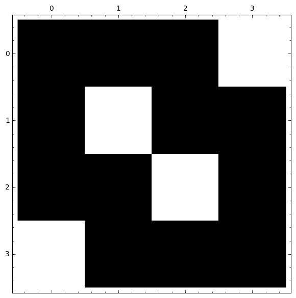
Figure 1: $[f_{2,1}]$: weight classes.     
    

Figure 2: $[f_{2,1}]$: extended Cayley classes.

As expected from Theorem 4, the two extended Cayley classes correspond to the two weight classes, as shown in Figures 1 and 2.

B.2 Bent functions in 4 dimensions

The bent functions on $\mathbb{F}_{2}^{4}$ consist of one EA class, containing the ET class $[f_{4,1}]$ where $f_{4,1}(x):=x_{0}x_{1}+x_{2}x_{3}$ is self dual. The ET class contains two extended Cayley classes as per Table 2.

$$\begin{array}[]{|cccl|}\hline\cr\text{Class}&\text{Parameters}&\text{2-rank}&\text{Clique polynomial}\\ \hline\cr 0&(16,6,2,2)&6&\begin{array}[]{l}8t^{4}+32t^{3}+48t^{2}+16t+1\end{array}\\ 1&(16,10,6,6)&6&\begin{array}[]{l}16t^{5}+120t^{4}+160t^{3}\,+\\ 80t^{2}+16t+1\end{array}\\ \hline\cr\end{array}$$

Table 2: $[f_{4,1}]$ extended Cayley classes.

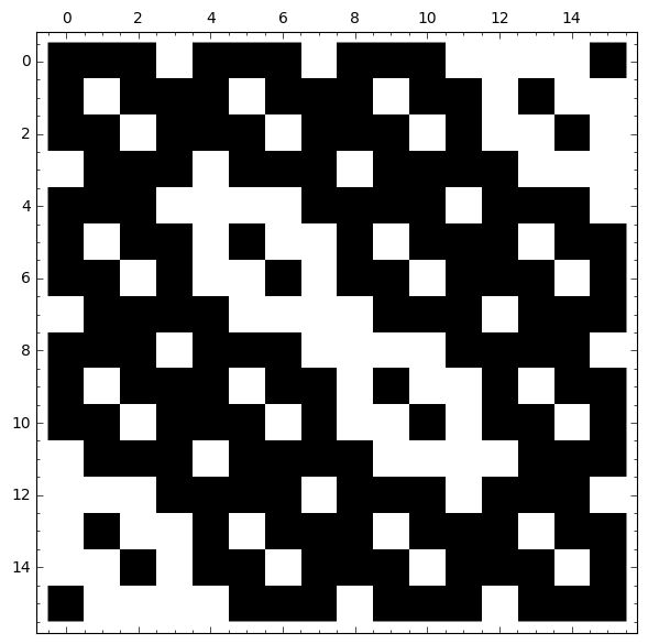
Figure 3: $[f_{4,1}]$: weight classes.     
    

Figure 4: $[f_{4,1}]$: extended Cayley classes.

The two extended Cayley classes correspond to the two weight classes, as shown in Figures 3 and 4.

B.3 Bent functions in 6 dimensions

Extended affine classes.

The bent functions on $\mathbb{F}_{2}^{6}$ consist of four EA classes, containing the ET classes as listed in Table 3 [55, p. 303] [65, Section 7.2].

$$\begin{array}[]{|cl|}\hline\cr\text{Class}&\text{Representative}\\ \hline\cr\,[f_{6,1}]&f_{6,1}:=\begin{array}[]{l}x_{0}x_{1}+x_{2}x_{3}+x_{4}x_{5}\end{array}\\ \,[f_{6,2}]&f_{6,2}:=\begin{array}[]{l}x_{0}x_{1}x_{2}+x_{0}x_{3}+x_{1}x_{4}+x_{2}x_{5}\end{array}\\ \,[f_{6,3}]&f_{6,3}:=\begin{array}[]{l}x_{0}x_{1}x_{2}+x_{0}x_{1}+x_{0}x_{3}+x_{1}x_{3}x_{4}+x_{1}x_{5}\,+\\ x_{2}x_{4}+x_{3}x_{4}\end{array}\\ \,[f_{6,4}]&f_{6,4}:=\begin{array}[]{l}x_{0}x_{1}x_{2}+x_{0}x_{3}+x_{1}x_{3}x_{4}+x_{1}x_{5}+x_{2}x_{3}x_{5}\,+\\ x_{2}x_{3}+x_{2}x_{4}+x_{2}x_{5}+x_{3}x_{4}+x_{3}x_{5}\end{array}\\ \hline\cr\end{array}$$

Table 3: 6 dimensions: ET classes.

In 1996, Tonchev classified the binary projective two-weight $[27,21,3]$ and $[35,6,16]$ codes listing them in Tables 1 and 2, respectively, of his paper [66]. These tables are repeated as Tables 1.155 and 1.156 in Chapter VII.1 of the Handbook of Combinatorial Designs, Second Edition [67], with a different numbering. For each of the codes listed in these two tables, the characteristics of the corresponding strongly regular graph is also listed.

In the classification given below, the Cayley graph of each Cayley class is matched by isomorphism with a strongly regular graph corresponding to one or more of Tonchev’s projective two-weight codes, or the complement of such a graph. Tonchev’s strongly regular graphs were checked using the function strongly_regular_from_two_weight_code, which uses the smaller of the two weights to create the graph [63].

ET class $[f_{6,1}]$.

This is the ET class of the bent function $f_{6,1}(x):=x_{0}x_{1}+x_{2}x_{3}+x_{4}x_{5}.$ This function is quadratic and self-dual.

The ET class contains two extended Cayley classes as per Table 4.

$$\begin{array}[]{|cccl|}\hline\cr\text{Class}&\text{Parameters}&\text{2-rank}&\text{Clique polynomial}\\ \hline\cr 0&(64,28,12,12)&8&\begin{array}[]{l}64t^{8}+512t^{7}+1792t^{6}+3584t^{5}\,+\\ 5376t^{4}+3584t^{3}+896t^{2}+64t+1\end{array}\\ 1&(64,36,20,20)&8&\begin{array}[]{l}2304t^{6}+13824t^{5}+19200t^{4}+7680t^{3}\,+\\ 1152t^{2}+64t+1\end{array}\\ \hline\cr\end{array}$$

Table 4: $[f_{6,1}]$ extended Cayley classes.

The Cayley graphs for classes 0 and 1 are isomorphic to those those obtained from Tonchev’s projective two-weight codes [67] as per Table 5.

$$\begin{array}[]{|ccl|}\hline\cr\text{Class}&\text{Parameters}&\text{Reference}\\ \hline\cr 0&[35,6,16]&\text{Table 1.156 1, 2 (complement)}\\ 1&[27,6,12]&\text{Table 1.155 1 }\\ \hline\cr\end{array}$$

Table 5: $[f_{6,1}]$ Two-weight projective codes.

The two extended Cayley classes correspond to the two weight classes, as shown in Figures 5 and 6.

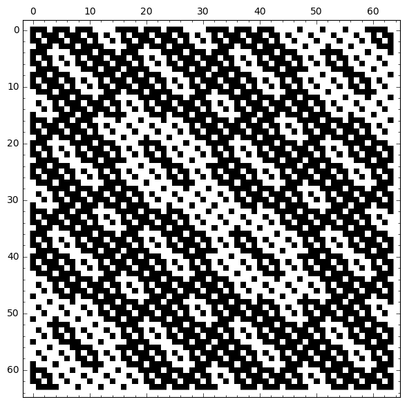
Figure 5: $[f_{6,1}]$: weight classes.     
    

Figure 6: $[f_{6,1}]$: extended Cayley classes.

Remark: The sequence of Figures 1, 3, and 5 displays a fractal-like self-similar quality.

ET class $[f_{6,2}]$.

This is the ET class of the bent function $f_{6,2}(x):=x_{0}x_{1}x_{2}+x_{0}x_{3}+x_{1}x_{4}+x_{2}x_{5}$.

The ET class contains three extended Cayley classes as per Table 6.

$$\begin{array}[]{|cccl|}\hline\cr\text{Class}&\text{Parameters}&\text{2-rank}&\text{Clique polynomial}\\ \hline\cr 0&(64,28,12,12)&8&\begin{array}[]{l}64t^{8}+512t^{7}+1792t^{6}+3584t^{5}\,+\\ 5376t^{4}+3584t^{3}+896t^{2}+64t+1\end{array}\\ 1&(64,28,12,12)&8&\begin{array}[]{l}256t^{6}+1536t^{5}+4352t^{4}+3584t^{3}\,+\\ 896t^{2}+64t+1\end{array}\\ 2&(64,36,20,20)&8&\begin{array}[]{l}192t^{8}+1536t^{7}+8960t^{6}+19968t^{5}\,+\\ 20224t^{4}+7680t^{3}+1152t^{2}+64t+1\end{array}\\ \hline\cr\end{array}$$

Table 6: $[f_{6,2}]$ extended Cayley classes.

The Cayley graph for class 0 is isomorphic to graph 0 of ET class $[f_{6,1}]$, This reflects the fact that $f_{6,1}\equiv f_{6,2}$, even though these two functions are not EA equivalent. This is therefore an example of an isomorphism between Cayley graphs of bent functions on $\mathbb{F}_{2}^{6}$ that is not a linear function.

The Cayley graph for class 0 is also isomorphic to the complement of Royle’s $(64,35,18,20)$ strongly regular graph $X$ [56].

The Cayley graphs for classes 0 to 2 are isomorphic to those those obtained from Tonchev’s projective two-weight codes [67] as per Table 7.

$$\begin{array}[]{|ccl|}\hline\cr\text{Class}&\text{Parameters}&\text{Reference}\\ \hline\cr 0&[35,6,16]&\text{Table 1.156 1, 2 (complement)}\\ 1&[35,6,16]&\text{Table 1.156 3 (complement)}\\ 2&[27,6,12]&\text{Table 1.155 2 }\\ \hline\cr\end{array}$$

Table 7: $[f_{6,2}]$ Two-weight projective codes.

The three extended Cayley classes are distributed between the two weight classes, as shown in Figures 7 and 8.

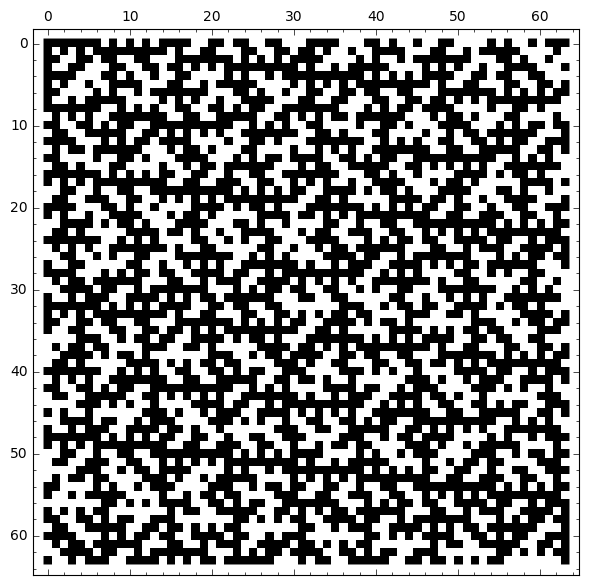
Figure 7: $[f_{6,2}]$: weight classes.     
    

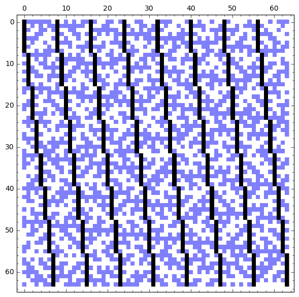
Figure 8: $[f_{6,2}]$: extended Cayley classes.

ET class $[f_{6,3}]$.

This is the ET class of the bent function

$$f_{6,3}(x) =x_{0}x_{1}x_{2}+x_{0}x_{1}+x_{0}x_{3}+x_{1}x_{3}x_{4}$$

$$+x_{1}x_{5}+x_{2}x_{4}+x_{3}x_{4}.$$

The ET class contains four extended Cayley classes as per Table 8.

$$\begin{array}[]{|cccl|}\hline\cr\text{Class}&\text{Parameters}&\text{2-rank}&\text{Clique polynomial}\\ \hline\cr 0&(64,28,12,12)&12&\begin{array}[]{l}32t^{8}+256t^{7}+896t^{6}+2048t^{5}+4608t^{4}\,+\\ 3584t^{3}+896t^{2}+64t+1\end{array}\\ 1&(64,36,20,20)&12&\begin{array}[]{l}160t^{8}+1280t^{7}+9344t^{6}+21504t^{5}\,+\\ 20480t^{4}+7680t^{3}+1152t^{2}+64t+1\end{array}\\ 2&(64,28,12,12)&12&\begin{array}[]{l}64t^{6}+1024t^{5}+4096t^{4}+3584t^{3}\,+\\ 896t^{2}+64t+1\end{array}\\ 3&(64,36,20,20)&12&\begin{array}[]{l}160t^{8}+1664t^{7}+9792t^{6}+21504t^{5}\,+\\ 20480t^{4}+7680t^{3}+1152t^{2}+64t+1\end{array}\\ \hline\cr\end{array}$$

Table 8: $[f_{6,3}]$ extended Cayley classes.

The Cayley graphs for classes 0 to 3 are isomorphic to those those obtained from Tonchev’s projective two-weight codes [67] as per Table 9.

$$\begin{array}[]{|ccl|}\hline\cr\text{Class}&\text{Parameters}&\text{Reference}\\ \hline\cr 0&[35,6,16]&\text{Table 1.156 4 (complement)}\\ 1&[27,6,12]&\text{Table 1.155 3 }\\ 2&[35,6,16]&\text{Table 1.156 5 (complement)}\\ 3&[27,6,12]&\text{Table 1.155 4 }\\ \hline\cr\end{array}$$

Table 9: $[f_{6,3}]$ Two-weight projective codes.

The four extended Cayley classes are distributed between the two weight classes, as shown in Figures 9 and 10.

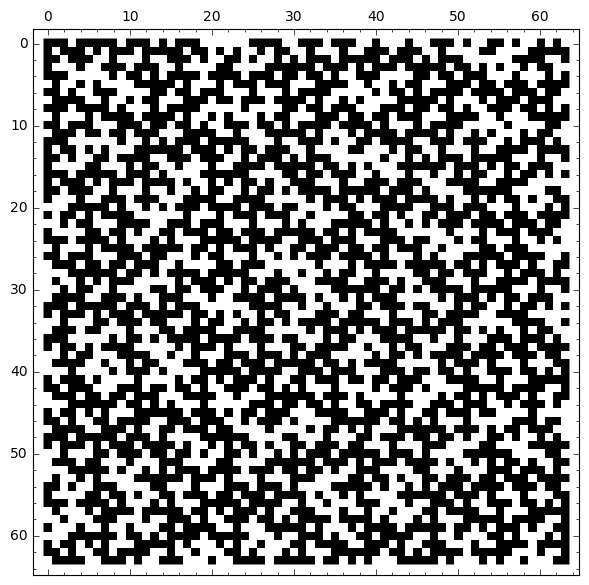
Figure 9: $[f_{6,3}]$: weight classes.     
    

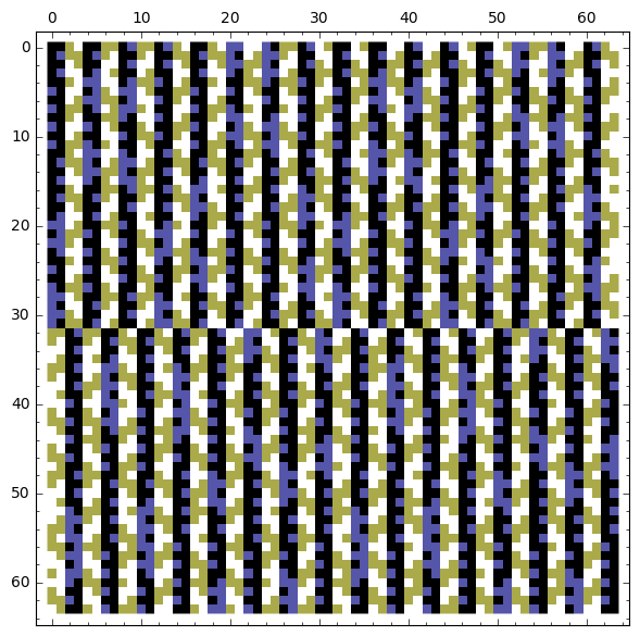
Figure 10: $[f_{6,3}]$: extended Cayley classes.

ET class $[f_{6,4}]$.

This is the ET class of the bent function

$$f_{6,4}(x) =x_{0}x_{1}x_{2}+x_{0}x_{3}+x_{1}x_{3}x_{4}+x_{1}x_{5}+x_{2}x_{3}x_{5}$$

$$+x_{2}x_{3}+x_{2}x_{4}+x_{2}x_{5}+x_{3}x_{4}+x_{3}x_{5}.$$

The ET class contains three extended Cayley classes as per Table 10.

$$\begin{array}[]{|cccl|}\hline\cr\text{Class}&\text{Parameters}&\text{2-rank}&\text{Clique polynomial}\\ \hline\cr 0&(64,28,12,12)&14&\begin{array}[]{l}32t^{8}+256t^{7}+896t^{6}+1792t^{5}+4480t^{4}\,+\\ 3584t^{3}+896t^{2}+64t+1\end{array}\\ 1&(64,28,12,12)&14&\begin{array}[]{l}16t^{8}+128t^{7}+448t^{6}+1280t^{5}+4224t^{4}\,+\\ 3584t^{3}+896t^{2}+64t+1\end{array}\\ 2&(64,36,20,20)&14&\begin{array}[]{l}176t^{8}+1408t^{7}+9664t^{6}+22272t^{5}\,+\\ 20608t^{4}+7680t^{3}+1152t^{2}+64t+1\end{array}\\ \hline\cr\end{array}$$

Table 10: $[f_{6,4}]$ extended Cayley classes.

The Cayley graphs for classes 0 to 2 are isomorphic to those those obtained from Tonchev’s projective two-weight codes [67] as per Table 11.

$$\begin{array}[]{|ccl|}\hline\cr\text{Class}&\text{Parameters}&\text{Reference}\\ \hline\cr 0&[35,6,16]&\text{Table 1.156 7 (complement)}\\ 1&[35,6,16]&\text{Table 1.156 6 (complement)}\\ 2&[27,6,12]&\text{Table 1.155 5 }\\ \hline\cr\end{array}$$

Table 11: $[f_{6,4}]$ Two-weight projective codes.

The three extended Cayley classes are distributed between the two weight classes, as shown in Figures 11 and 12.

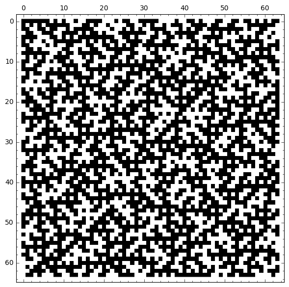
Figure 11: $[f_{6,4}]$: weight classes.     
    

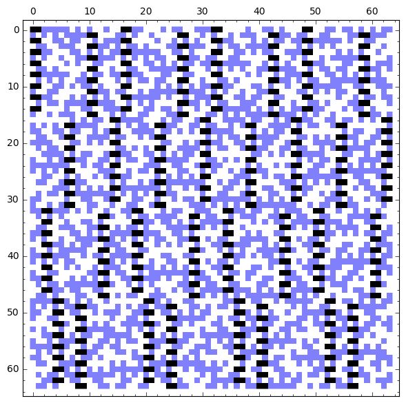
Figure 12: $[f_{6,4}]$: extended Cayley classes.

B.4 Bent functions in 8 dimensions

There are $99\,270\,589\,265\,934\,370\,305\,785\,861\,242\,880\approx 2^{106}$ bent functions in 8 dimensions, according to Langevin and Leander [37]. The number of EA classes has not yet been published, let alone a list of representative bent functions. The lists of EA classes of bent functions that have so far been published include those for the bent functions of degree at most 3 [8, Section 5.5.2] [65, Section 7.3], and the partial spread bent functions [35, 36]. The bent functions used in the S-boxes of the CAST-128 encryption algorithm [2, 1] are also representatives of disjoint EA classes.

Extended affine classes of degree at most 3.

According to a list contained in Braeken’s PhD thesis [8, Section 5.5.2], and repeated in Tokareva’s table [65, Section 7.3], the bent functions on $\mathbb{F}_{2}^{8}$, of degree at most 3, consist of 10 EA classes, whose representatives are listed in Table 12.

$$\begin{array}[]{|cl|}\hline\cr\text{Class}&\text{Representative}\\ \hline\cr\,[f_{8,1}]&f_{8,1}:=\begin{array}[]{l}x_{0}x_{1}+x_{2}x_{3}+x_{4}x_{5}+x_{6}x_{7}\end{array}\\ \,[f_{8,2}]&f_{8,2}:=\begin{array}[]{l}x_{0}x_{1}x_{2}+x_{0}x_{3}+x_{1}x_{4}+x_{2}x_{5}+x_{6}x_{7}\end{array}\\ \,[f_{8,3}]&f_{8,3}:=\begin{array}[]{l}x_{0}x_{1}x_{2}+x_{0}x_{6}+x_{1}x_{3}x_{4}+x_{1}x_{5}+x_{2}x_{3}+x_{4}x_{7}\end{array}\\ \,[f_{8,4}]&f_{8,4}:=\begin{array}[]{l}x_{0}x_{1}x_{2}+x_{0}x_{2}+x_{0}x_{4}+x_{1}x_{3}x_{4}+x_{1}x_{5}+x_{2}x_{3}\,+x_{6}x_{7}\end{array}\\ \,[f_{8,5}]&f_{8,5}:=\begin{array}[]{l}x_{0}x_{1}x_{2}+x_{0}x_{6}+x_{1}x_{3}x_{4}+x_{1}x_{4}+x_{1}x_{5}+x_{2}x_{3}x_{5}+x_{2}x_{4}+x_{3}x_{7}\end{array}\\ \,[f_{8,6}]&f_{8,6}:=\begin{array}[]{l}x_{0}x_{1}x_{2}+x_{0}x_{2}+x_{0}x_{3}+x_{1}x_{3}x_{4}+x_{1}x_{6}+x_{2}x_{3}x_{5}+x_{2}x_{4}+x_{5}x_{7}\end{array}\\ \,[f_{8,7}]&f_{8,7}:=\begin{array}[]{l}x_{0}x_{1}x_{2}+x_{0}x_{1}+x_{0}x_{2}+x_{0}x_{3}+x_{1}x_{3}x_{4}+x_{1}x_{4}\,+x_{1}x_{5}\,+\\ x_{2}x_{3}x_{5}+x_{2}x_{4}+x_{6}x_{7}\end{array}\\ \,[f_{8,8}]&f_{8,8}:=\begin{array}[]{l}x_{0}x_{1}x_{2}+x_{0}x_{5}+x_{1}x_{3}x_{4}+x_{1}x_{6}+x_{2}x_{3}x_{5}+x_{2}x_{4}+x_{3}x_{7}\end{array}\\ \,[f_{8,9}]&f_{8,9}:=\begin{array}[]{l}x_{0}x_{1}x_{6}+x_{0}x_{3}+x_{1}x_{4}+x_{2}x_{3}x_{6}+x_{2}x_{5}+x_{3}x_{4}\,+x_{4}x_{5}x_{6}+x_{6}x_{7}\end{array}\\ \,[f_{8,10}]&f_{8,10}:=\begin{array}[]{l}x_{0}x_{1}x_{2}+x_{0}x_{3}x_{6}+x_{0}x_{4}+x_{0}x_{5}+x_{1}x_{3}x_{4}+x_{1}x_{6}+x_{2}x_{3}x_{5}\,+\\ x_{2}x_{4}+x_{3}x_{7}\end{array}\\ \hline\cr\end{array}$$

Table 12: 8 dimensions to degree 3: ET classes.

We here examine the corresponding ET classes in detail.

ET class $[f_{8,1}]$.

This is the ET class of the bent function

$$f_{8,1} =\begin{array}[]{l}x_{0}x_{1}+x_{2}x_{3}+x_{4}x_{5}+x_{6}x_{7}.\end{array}$$

This function is quadratic and self-dual. The ET class contains two extended Cayley classes as per Table 13.

$$\begin{array}[]{|cccl|}\hline\cr\text{Class}&\text{Parameters}&\text{2-rank}&\text{Clique polynomial}\\ \hline\cr 0&(256,120,56,56)&10&\begin{array}[]{l}245760t^{9}+3317760t^{8}+8847360t^{7}\,+\\ 10321920t^{6}+6193152t^{5}+2007040t^{4}\,+\\ 286720t^{3}+15360t^{2}+256t+1\end{array}\\ 1&(256,136,72,72)&10&\begin{array}[]{l}417792t^{8}+3342336t^{7}+11698176t^{6}\,+\\ 11698176t^{5}+3760128t^{4}+417792t^{3}\,+\\ 17408t^{2}+256t+1\end{array}\\ \hline\cr\end{array}$$

Table 13: $[f_{8,1}]$ extended Cayley classes.

As expected from Theorem 4, the two extended Cayley classes correspond to the two weight classes, as shown in Figures 13 and 14.

Remark: The fractal-like self-similar quality of Figures 1, 3, and 5 continues with Figure 13.

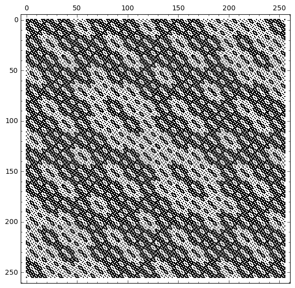
Figure 13: $[f_{8,1}]$: weight classes.     
    

Figure 14: $[f_{8,1}]$: extended Cayley classes.

ET class $[f_{8,2}]$.

This is the ET class of the bent function

$$f_{8,2} =\begin{array}[]{l}x_{0}x_{1}x_{2}+x_{0}x_{3}+x_{1}x_{4}+x_{2}x_{5}+x_{6}x_{7}.\end{array}$$

The ET class contains four extended Cayley classes as per Table 14.

$$\begin{array}[]{|cccl|}\hline\cr\text{Class}&\text{Parameters}&\text{2-rank}&\text{Clique polynomial}\\ \hline\cr 0&(256,120,56,56)&10&\begin{array}[]{l}245760t^{9}+3317760t^{8}+8847360t^{7}\,+\\ 10321920t^{6}+6193152t^{5}+2007040t^{4}\,+\\ 286720t^{3}+15360t^{2}+256t+1\end{array}\\ 1&(256,120,56,56)&10&\begin{array}[]{l}49152t^{9}+663552t^{8}+2555904t^{7}\,+\\ 5079040t^{6}+4620288t^{5}+1875968t^{4}\,+\\ 286720t^{3}+15360t^{2}+256t+1\end{array}\\ 2&(256,136,72,72)&10&\begin{array}[]{l}327680t^{9}+4055040t^{8}+13828096t^{7}\,+\\ 22183936t^{6}+14319616t^{5}+3891200t^{4}\,+\\ 417792t^{3}+17408t^{2}+256t+1\end{array}\\ 3&(256,136,72,72)&10&\begin{array}[]{l}417792t^{8}+3342336t^{7}+11698176t^{6}\,+\\ 11698176t^{5}+3760128t^{4}+417792t^{3}\,+\\ 17408t^{2}+256t+1\end{array}\\ \hline\cr\end{array}$$

Table 14: $[f_{8,2}]$ extended Cayley classes.

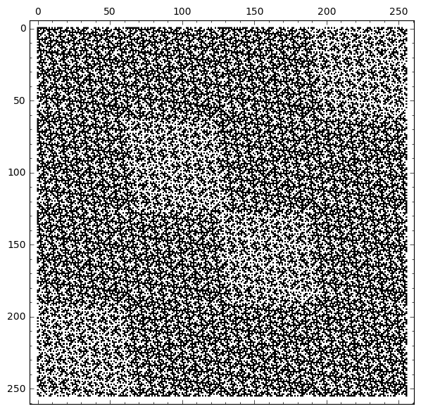
Figure 15: $[f_{8,2}]$: weight classes.     
    

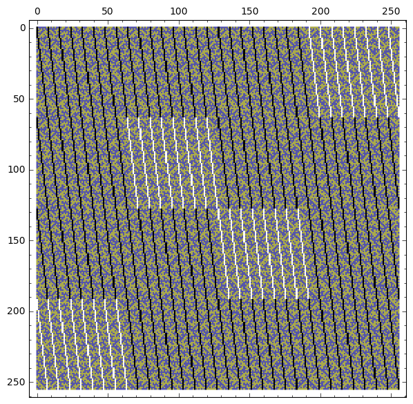
Figure 16: $[f_{8,2}]$: extended Cayley classes.

The Cayley graph for class 0 is isomorphic to graph 0 of ET class $[f_{8,1}]$, This reflects the fact that $f_{8,1}\equiv f_{8,2}$, even though these two functions are not EA equivalent. This is therefore an example of an isomorphism between Cayley graphs of bent functions on $\mathbb{F}_{2}^{8}$ that is not a linear function.

The four extended Cayley classes are distributed between the two weight classes, as shown in Figures 15 and 16.

ET class $[f_{8,3}]$.

This is the ET class of the bent function

$$f_{8,3} =\begin{array}[]{l}x_{0}x_{1}x_{2}+x_{0}x_{6}+x_{1}x_{3}x_{4}+x_{1}x_{5}+x_{2}x_{3}+x_{4}x_{7}.\end{array}$$

The ET class contains six extended Cayley classes as per Table 15.

$$\begin{array}[]{|cccl|}\hline\cr\text{Class}&\text{Parameters}&\text{2-rank}&\text{Clique polynomial}\\ \hline\cr 0&(256,120,56,56)&12&\begin{array}[]{l}81920t^{9}+1368064t^{8}+4653056t^{7}\,+\\ 7176192t^{6}+5406720t^{5}+1941504t^{4}\,+\\ 286720t^{3}+15360t^{2}+256t+1\end{array}\\ 1&(256,136,72,72)&12&\begin{array}[]{l}294912t^{9}+6299648t^{8}+21692416t^{7}\,+\\ 27951104t^{6}+15630336t^{5}+3956736t^{4}\,+\\ 417792t^{3}+17408t^{2}+256t+1\end{array}\\ 2&(256,120,56,56)&12&\begin{array}[]{l}16384t^{9}+221184t^{8}+1277952t^{7}\,+\\ 3768320t^{6}+4227072t^{5}+1843200t^{4}\,+\\ 286720t^{3}+15360t^{2}+256t+1\end{array}\\ 3&(256,136,72,72)&12&\begin{array}[]{l}262144t^{9}+4399104t^{8}+16220160t^{7}\,+\\ 24281088t^{6}+14974976t^{5}+3923968t^{4}\,+\\ 417792t^{3}+17408t^{2}+256t+1\end{array}\\ 4&(256,120,56,56)&12&\begin{array}[]{l}49152t^{9}+729088t^{8}+2686976t^{7}\,+\\ 5079040t^{6}+4620288t^{5}+1875968t^{4}\,+\\ 286720t^{3}+15360t^{2}+256t+1\end{array}\\ 5&(256,136,72,72)&12&\begin{array}[]{l}196608t^{9}+3399680t^{8}+13172736t^{7}\,+\\ 21659648t^{6}+14319616t^{5}+3891200t^{4}\,+\\ 417792t^{3}+17408t^{2}+256t+1\end{array}\\ \hline\cr\end{array}$$

Table 15: $[f_{8,3}]$ extended Cayley classes.

The six extended Cayley classes are distributed between the two weight classes, as shown in Figures 17 and 18.

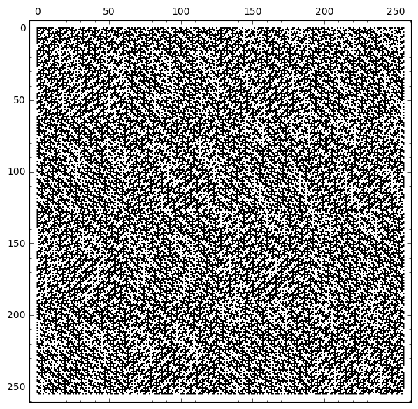
Figure 17: $[f_{8,3}]$: weight classes.     
    

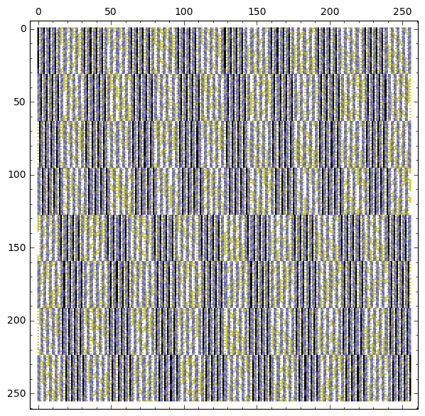
Figure 18: $[f_{8,3}]$: extended Cayley classes.

ET class $[f_{8,4}]$.

This is the ET class of the bent function

$$f_{8,4} =\begin{array}[]{l}x_{0}x_{1}x_{2}+x_{0}x_{2}+x_{0}x_{4}+x_{1}x_{3}x_{4}+x_{1}x_{5}+x_{2}x_{3}\,+x_{6}x_{7}.\end{array}$$

The ET class contains six extended Cayley classes as per Table 16.

The six extended Cayley classes are distributed between the two weight classes, as shown in Figures 19 and 20.

$$\begin{array}[]{|cccl|}\hline\cr\text{Class}&\text{Parameters}&\text{2-rank}&\text{Clique polynomial}\\ \hline\cr 0&(256,120,56,56)&14&\begin{array}[]{l}69632t^{9}+1099776t^{8}+3784704t^{7}\,+\\ 6160384t^{6}+5013504t^{5}+1908736t^{4}\,+\\ 286720t^{3}+15360t^{2}+256t+1\end{array}\\ 1&(256,136,72,72)&14&\begin{array}[]{l}225280t^{9}+4319232t^{8}+16203776t^{7}\,+\\ 24313856t^{6}+14974976t^{5}+3923968t^{4}\,+\\ 417792t^{3}+17408t^{2}+256t+1\end{array}\\ 2&(256,120,56,56)&14&\begin{array}[]{l}1536t^{10}+15360t^{9}+209920t^{8}\,+\\ 1280000t^{7}+3751936t^{6}+4227072t^{5}\,+\\ 1843200t^{4}+286720t^{3}+15360t^{2}+256t+1\end{array}\\ 3&(256,136,72,72)&14&\begin{array}[]{l}7680t^{10}+230400t^{9}+4228096t^{8}\,+\\ 16058368t^{7}+24166400t^{6}+14974976t^{5}\,+\\ 3923968t^{4}+417792t^{3}+17408t^{2}+256t+1\end{array}\\ 4&(256,136,72,72)&14&\begin{array}[]{l}110592t^{9}+2344960t^{8}+10305536t^{7}\,+\\ 18939904t^{6}+13664256t^{5}+3858432t^{4}\,+\\ 417792t^{3}+17408t^{2}+256t+1\end{array}\\ 5&(256,120,56,56)&14&\begin{array}[]{l}20480t^{9}+337920t^{8}+1556480t^{7}\,+\\ 3932160t^{6}+4227072t^{5}+1843200t^{4}\,+\\ 286720t^{3}+15360t^{2}+256t+1\end{array}\\ \hline\cr\end{array}$$

Table 16: $[f_{8,4]}$ extended Cayley classes.

Figure 19: $[f_{8,4}]$: weight classes.     
    

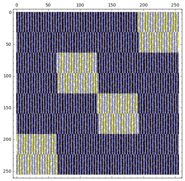
Figure 20: $[f_{8,4}]$: extended Cayley classes.

ET class $[f_{8,5}]$.

This is the ET class of the bent function

$$f_{8,5} =\begin{array}[]{l}x_{0}x_{1}x_{2}+x_{0}x_{6}+x_{1}x_{3}x_{4}+x_{1}x_{4}+x_{1}x_{5}+x_{2}x_{3}x_{5}+x_{2}x_{4}+x_{3}x_{7}.\end{array}$$

The ET class contains 9 extended Cayley classes as per Table 17.

$$\begin{array}[]{|cccl|}\hline\cr\text{Class}&\text{Parameters}&\text{2-rank}&\text{Clique polynomial}\\ \hline\cr 0&(256,120,56,56)&14&\begin{array}[]{l}32768t^{9}+731136t^{8}+3096576t^{7}\,+\\ 5767168t^{6}+5013504t^{5}+1908736t^{4}\,+\\ 286720t^{3}+15360t^{2}+256t+1\end{array}\\ 1&(256,120,56,56)&14&\begin{array}[]{l}28672t^{9}+534528t^{8}+2211840t^{7}\,+\\ 4718592t^{6}+4620288t^{5}+1875968t^{4}\,+\\ 286720t^{3}+15360t^{2}+256t+1\end{array}\\ 2&(256,136,72,72)&14&\begin{array}[]{l}159744t^{9}+4753408t^{8}+19021824t^{7}\,+\\ 26804224t^{6}+15630336t^{5}+3956736t^{4}\,+\\ 417792t^{3}+17408t^{2}+256t+1\end{array}\\ 3&(256,120,56,56)&14&\begin{array}[]{l}24576t^{9}+526336t^{8}+2342912t^{7}\,+\\ 4849664t^{6}+4620288t^{5}+1875968t^{4}\,+\\ 286720t^{3}+15360t^{2}+256t+1\end{array}\\ 4&(256,136,72,72)&14&\begin{array}[]{l}90112t^{9}+2795520t^{8}+12402688t^{7}\,+\\ 21168128t^{6}+14319616t^{5}+3891200t^{4}\,+\\ 417792t^{3}+17408t^{2}+256t+1\end{array}\\ 5&(256,120,56,56)&14&\begin{array}[]{l}16384t^{9}+284672t^{8}+1392640t^{7}\,+\\ 3735552t^{6}+4227072t^{5}+1843200t^{4}\,+\\ 286720t^{3}+15360t^{2}+256t+1\end{array}\\ 6&(256,136,72,72)&14&\begin{array}[]{l}131072t^{9}+3577856t^{8}+15319040t^{7}\,+\\ 23855104t^{6}+14974976t^{5}+3923968t^{4}\,+\\ 417792t^{3}+17408t^{2}+256t+1\end{array}\\ 7&(256,120,56,56)&14&\begin{array}[]{l}1536t^{10}+19456t^{9}+279552t^{8}\,+\\ 1394688t^{7}+3751936t^{6}+4227072t^{5}\,+\\ 1843200t^{4}+286720t^{3}+15360t^{2}+256t+1\end{array}\\ 8&(256,136,72,72)&14&\begin{array}[]{l}5632t^{10}+148480t^{9}+3621888t^{8}\,+\\ 15206400t^{7}+23773184t^{6}+14974976t^{5}\,+\\ 3923968t^{4}+417792t^{3}+17408t^{2}+256t+1\end{array}\\ \hline\cr\end{array}$$

Table 17: $[f_{8,5}]$ extended Cayley classes.

The 9 extended Cayley classes are distributed between the two weight classes, as shown in Figures 21 and 22.

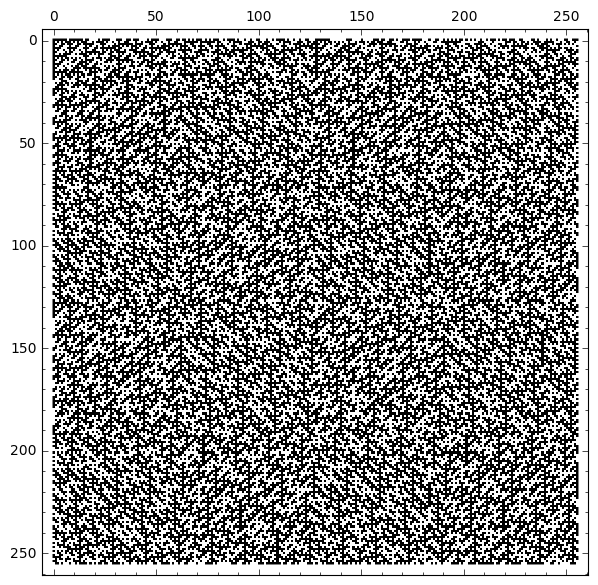
Figure 21: $[f_{8,5}]$: weight classes.     
    

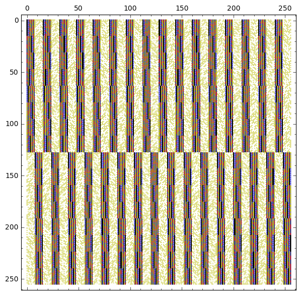
Figure 22: $[f_{8,5}]$: extended Cayley classes.

ET class $[f_{8,6}]$.

This is the ET class of the bent function

$$f_{8,6} =\begin{array}[]{l}x_{0}x_{1}x_{2}+x_{0}x_{2}+x_{0}x_{3}+x_{1}x_{3}x_{4}+x_{1}x_{6}+x_{2}x_{3}x_{5}+x_{2}x_{4}+x_{5}x_{7}.\end{array}$$

The ET class contains 9 extended Cayley classes.

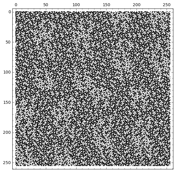
Figure 23: $[f_{8,6}]$: weight classes.     
    

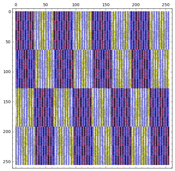
Figure 24: $[f_{8,6}]$: extended Cayley classes.

The 9 extended Cayley classes are distributed between the two weight classes, as shown in Figures 23 and 24.

The 9 Cayley graphs corresponding to the 9 classes are isomorphic to those for the extended Cayley classes for $[f_{8,5}]$. The corresponding Cayley classes have the same frequency within each of these two ET classes. This correspondence is shown in Table 18.

Figures 25 and 25 show the 9 extended Cayley classes of each of $[f_{8,5}]$ and $[f_{8,6}]$ with corresponding Cayley classes given the same colour.

$$\begin{array}[]{|ccr|}\hline\cr[f_{8,5}]&[f_{8,6}]&\text{Frequency}\\ \hline\cr 0&0&4096\\ 1&1&6144\\ 2&2&6144\\ 3&5&2048\\ 4&8&2048\\ 5&6&6144\\ 6&7&6144\\ 7&3&16384\\ 8&4&16384\\ \hline\cr\end{array}$$

Table 18: Correspondence between $[f_{8,5}]$ and $[f_{8,6}]$ extended Cayley classes.

Figure 25: $[f_{8,5}]$: extended Cayley classes (recoloured).

Figure 26: $[f_{8,6}]$: extended Cayley classes (recoloured).

The explanation for the correspondence between the Cayley classes of $f_{8,5}$ and $f_{8,6}$ is quite simple. The functions $f_{8,5}$ and $f_{8,6}$ are EA equivalent, in fact general linear equivalent, and therefore Braeken’s list of EA equivalence classes [8, Section 5.5.2] contains an error.

Theorem 6.

Functions $f_{8,5}$ and $f_{8,6}$ are general linear equivalent.

Proof.

Apply the permutation $\pi:=(x_{0}\ x_{5}\ x_{4})(x_{1}\ x_{2}\ x_{3})(x_{6}\ x_{7})$ to

$$f_{8,5} =x_{0}x_{1}x_{2}+x_{0}x_{6}+x_{1}x_{3}x_{4}+x_{1}x_{4}+x_{1}x_{5}+x_{2}x_{3}x_{5}+x_{2}x_{4}+x_{3}x_{7}$$

to obtain

$$\pi(f_{8,5}) =x_{5}x_{2}x_{3}+x_{5}x_{7}+x_{2}x_{1}x_{0}+x_{2}x_{0}+x_{2}x_{4}+x_{3}x_{1}x_{4}+x_{3}x_{0}+x_{1}x_{6}$$

$$=x_{0}x_{1}x_{2}+x_{0}x_{2}+x_{0}x_{3}+x_{1}x_{3}x_{4}+x_{1}x_{6}+x_{2}x_{3}x_{5}+x_{2}x_{4}+x_{5}x_{7}$$

$$=f_{8,6}.$$

∎

ET class $[f_{8,7}]$.

This is the ET class of the bent function

$$f_{8,7} =\begin{array}[]{l}x_{0}x_{1}x_{2}+x_{0}x_{1}+x_{0}x_{2}+x_{0}x_{3}+x_{1}x_{3}x_{4}+x_{1}x_{4}\,+x_{1}x_{5}\,+\\ x_{2}x_{3}x_{5}+x_{2}x_{4}+x_{6}x_{7}.\end{array}$$

The ET class contains six extended Cayley classes as per Table 19.

The six extended Cayley classes are distributed between the two weight classes, as shown in Figures 27 and 28.

$$\begin{array}[]{|cccl|}\hline\cr\text{Class}&\text{Parameters}&\text{2-rank}&\text{Clique polynomial}\\ \hline\cr 0&(256,120,56,56)&16&\begin{array}[]{l}29696t^{9}+655360t^{8}+2789376t^{7}\,+\\ 5332992t^{6}+4816896t^{5}+1892352t^{4}\,+\\ 286720t^{3}+15360t^{2}+256t+1\end{array}\\ 1&(256,120,56,56)&16&\begin{array}[]{l}20480t^{9}+409600t^{8}+1837056t^{7}\,+\\ 4235264t^{6}+4423680t^{5}+1859584t^{4}\,+\\ 286720t^{3}+15360t^{2}+256t+1\end{array}\\ 2&(256,136,72,72)&16&\begin{array}[]{l}143360t^{9}+3981312t^{8}+16697344t^{7}\,+\\ 25108480t^{6}+15302656t^{5}+3940352t^{4}\,+\\ 417792t^{3}+17408t^{2}+256t+1\end{array}\\ 3&(256,136,72,72)&16&\begin{array}[]{l}64512t^{9}+2316288t^{8}+10932224t^{7}\,+\\ 19783680t^{6}+13991936t^{5}+3874816t^{4}\,+\\ 417792t^{3}+17408t^{2}+256t+1\end{array}\\ 4&(256,136,72,72)&16&\begin{array}[]{l}92160t^{9}+2979840t^{8}+13608960t^{7}\,+\\ 22388736t^{6}+14647296t^{5}+3907584t^{4}\,+\\ 417792t^{3}+17408t^{2}+256t+1\end{array}\\ 5&(256,120,56,56)&16&\begin{array}[]{l}6144t^{9}+124928t^{8}+944128t^{7}\,+\\ 3219456t^{6}+4030464t^{5}+1826816t^{4}\,+\\ 286720t^{3}+15360t^{2}+256t+1\end{array}\\ \hline\cr\end{array}$$

Table 19: $[f_{8,7}]$ extended Cayley classes.

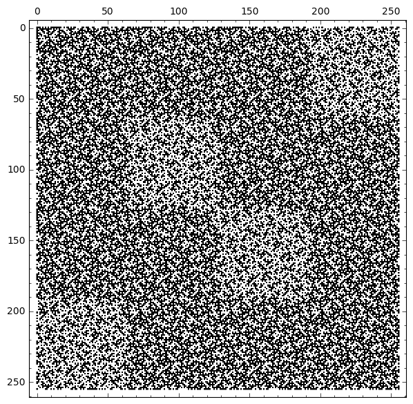
Figure 27: $[f_{8,7}]$: weight classes.     
    

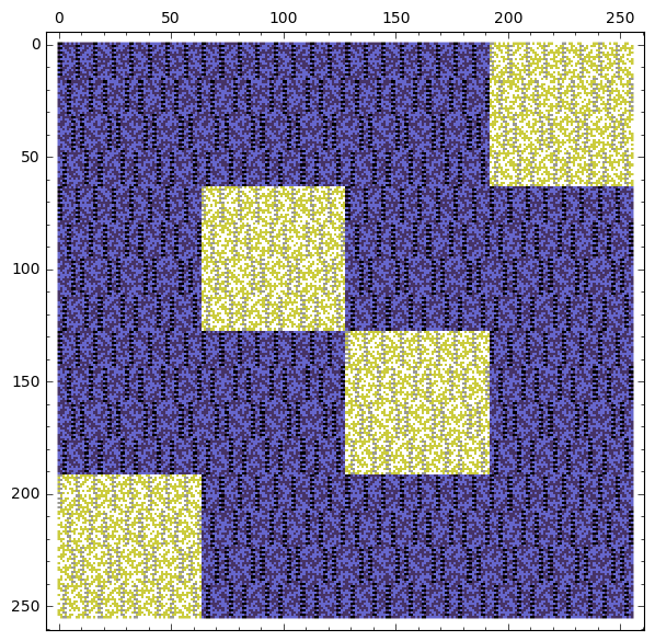
Figure 28: $[f_{8,7}]$: extended Cayley classes.

ET class $[f_{8,8}]$.

This is the ET class of the bent function

$$f_{8,8} =\begin{array}[]{l}x_{0}x_{1}x_{2}+x_{0}x_{5}+x_{1}x_{3}x_{4}+x_{1}x_{6}+x_{2}x_{3}x_{5}+x_{2}x_{4}+x_{3}x_{7}.\end{array}$$

The ET class contains six extended Cayley classes as per Table 20.

The six extended Cayley classes are distributed between the two weight classes, as shown in Figures 29 and 30.

$$\begin{array}[]{|cccl|}\hline\cr\text{Class}&\text{Parameters}&\text{2-rank}&\text{Clique polynomial}\\ \hline\cr 0&(256,120,56,56)&14&\begin{array}[]{l}32768t^{9}+712704t^{8}+3014656t^{7}\,+\\ 5734400t^{6}+5013504t^{5}+1908736t^{4}\,+\\ 286720t^{3}+15360t^{2}+256t+1\end{array}\\ 1&(256,120,56,56)&14&\begin{array}[]{l}24576t^{9}+466944t^{8}+2064384t^{7}\,+\\ 4685824t^{6}+4620288t^{5}+1875968t^{4}\,+\\ 286720t^{3}+15360t^{2}+256t+1\end{array}\\ 2&(256,136,72,72)&14&\begin{array}[]{l}172032t^{9}+5332992t^{8}+20283392t^{7}\,+\\ 27295744t^{6}+15630336t^{5}+3956736t^{4}\,+\\ 417792t^{3}+17408t^{2}+256t+1\end{array}\\ 3&(256,136,72,72)&14&\begin{array}[]{l}147456t^{9}+3858432t^{8}+15990784t^{7}\,+\\ 24150016t^{6}+14974976t^{5}+3923968t^{4}\,+\\ 417792t^{3}+17408t^{2}+256t+1\end{array}\\ 4&(256,120,56,56)&14&\begin{array}[]{l}16384t^{9}+270336t^{8}+1376256t^{7}\,+\\ 3768320t^{6}+4227072t^{5}+1843200t^{4}\,+\\ 286720t^{3}+15360t^{2}+256t+1\end{array}\\ 5&(256,136,72,72)&14&\begin{array}[]{l}163840t^{9}+3858432t^{8}+15532032t^{7}\,+\\ 23887872t^{6}+14974976t^{5}+3923968t^{4}\,+\\ 417792t^{3}+17408t^{2}+256t+1\end{array}\\ \hline\cr\end{array}$$

Table 20: $[f_{8,8}]$ extended Cayley classes.

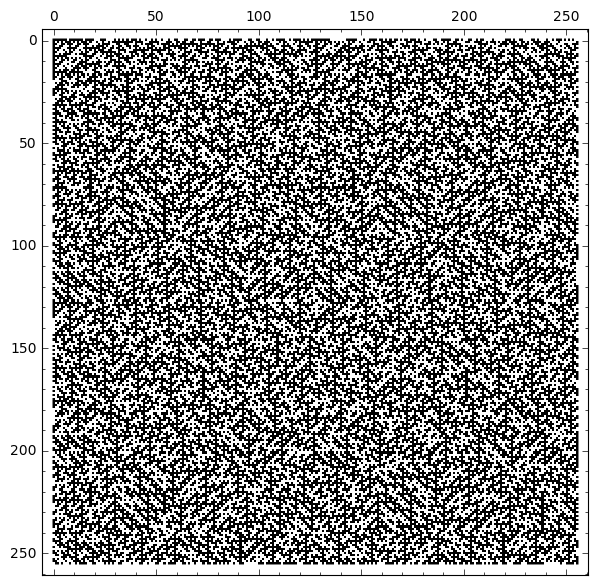
Figure 29: $[f_{8,8}]$: weight classes.     
    

Figure 30: $[f_{8,8}]$: extended Cayley classes.

ET class $[f_{8,9}]$.

This is the ET class of the bent function

$$f_{8,9} =\begin{array}[]{l}x_{0}x_{1}x_{6}+x_{0}x_{3}+x_{1}x_{4}+x_{2}x_{3}x_{6}+x_{2}x_{5}+x_{3}x_{4}\,+x_{4}x_{5}x_{6}+x_{6}x_{7}.\end{array}$$

The ET class contains 8 extended Cayley classes as per Table 21. In 4 of these 8 classes, each bent function is extended Cayley equivalent to its dual. In the remaining 4 extended Cayley classes, the dual of every bent function in the class has a Cayley graph that is isomorphic to that of one other class. That is, the 4 Cayley classes form two duality pairs of classes. This correspondence between Cayley classes and Cayley classes of duals is shown in Table 22.

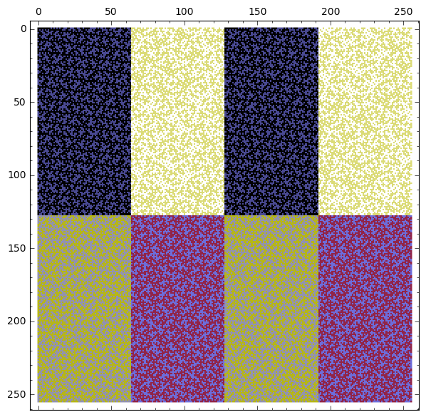
Figure 31: $[f_{8,9}]$: 8 extended Cayley classes                       

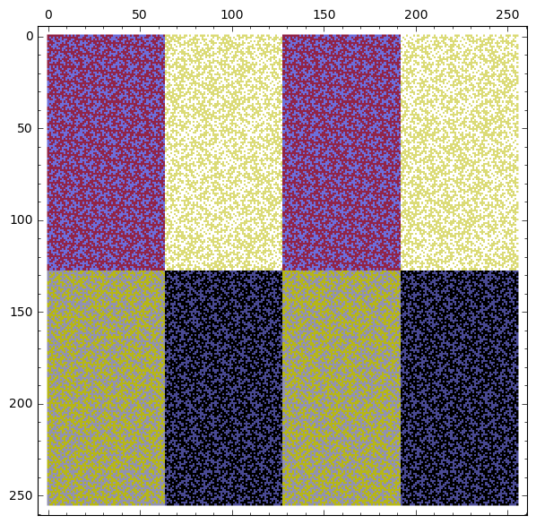
Figure 32: $[f_{8,9}]$: 8 extended Cayley classes of dual bent functions

The 8 extended Cayley classes are distributed as shown in Figures 31 (classes) and 32 (classes of duals).

$$\begin{array}[]{|cccl|}\hline\cr\text{Class}&\text{Parameters}&\text{2-rank}&\text{Clique polynomial}\\ \hline\cr 0&(256,120,56,56)&16&\begin{array}[]{l}45056t^{9}+780288t^{8}+2998272t^{7}\,+\\ 5505024t^{6}+4816896t^{5}+1892352t^{4}\,+\\ 286720t^{3}+15360t^{2}+256t+1\end{array}\\ 1&(256,120,56,56)&16&\begin{array}[]{l}45056t^{9}+780288t^{8}+2998272t^{7}\,+\\ 5505024t^{6}+4816896t^{5}+1892352t^{4}\,+\\ 286720t^{3}+15360t^{2}+256t+1\end{array}\\ 2&(256,136,72,72)&16&\begin{array}[]{l}184320t^{9}+3852288t^{8}+14893056t^{7}\,+\\ 23003136t^{6}+14647296t^{5}+3907584t^{4}\,+\\ 417792t^{3}+17408t^{2}+256t+1\end{array}\\ 3&(256,136,72,72)&16&\begin{array}[]{l}184320t^{9}+3852288t^{8}+14893056t^{7}\,+\\ 23003136t^{6}+14647296t^{5}+3907584t^{4}\,+\\ 417792t^{3}+17408t^{2}+256t+1\end{array}\\ 4&(256,120,56,56)&16&\begin{array}[]{l}105984t^{8}+976896t^{7}+3440640t^{6}\,+\\ 4128768t^{5}+1835008t^{4}+286720t^{3}\,+\\ 15360t^{2}+256t+1\end{array}\\ 5&(256,136,72,72)&16&\begin{array}[]{l}9216t^{10}+264192t^{9}+4468224t^{8}\,+\\ 16803840t^{7}+24772608t^{6}+15138816t^{5}\,+\\ 3932160t^{4}+417792t^{3}+17408t^{2}+256t+1\end{array}\\ 6&(256,120,56,56)&16&\begin{array}[]{l}9216t^{9}+124416t^{8}+976896t^{7}\,+\\ 3440640t^{6}+4128768t^{5}+1835008t^{4}\,+\\ 286720t^{3}+15360t^{2}+256t+1\end{array}\\ 7&(256,136,72,72)&16&\begin{array}[]{l}193536t^{9}+4449792t^{8}+16803840t^{7}\,+\\ 24772608t^{6}+15138816t^{5}+3932160t^{4}\,+\\ 417792t^{3}+17408t^{2}+256t+1\end{array}\\ \hline\cr\end{array}$$

Table 21: $[f_{8,9}]$ extended Cayley classes.

$$\begin{array}[]{|ccc|}\hline\cr[f_{8,9}]&[f_{8,9}]&\text{Frequency}\\ &\text{duals}&\\ \hline\cr 0&1&9216\\ 1&0&9216\\ 2&3&7168\\ 3&2&7168\\ 4&4&8192\\ 5&5&8192\\ 6&6&8192\\ 7&7&8192\\ \hline\cr\end{array}$$

Table 22: Correspondence between $[f_{8,9}]$ extended Cayley classes and $[f_{8,9}]$ dual extended Cayley classes.

ET class $[f_{8,10}]$.

This is the ET class of the bent function

$$f_{8,10}:=\begin{array}[]{l}x_{0}x_{1}x_{2}+x_{0}x_{3}x_{6}+x_{0}x_{4}+x_{0}x_{5}+x_{1}x_{3}x_{4}+x_{1}x_{6}+x_{2}x_{3}x_{5}\,+\\ x_{2}x_{4}+x_{3}x_{7}.\end{array}$$

The ET class contains 10 extended Cayley classes as per Table 23. In 4 of these 10 classes, each bent function is extended Cayley equivalent to its dual. In the remaining 6 extended Cayley classes, the dual of every bent function in the class has a Cayley graph that is isomorphic to that of one other class. That is, the 6 Cayley classes form three duality pairs of classes. This correspondence between Cayley classes and Cayley classes of duals is shown in Table 24.

The 10 extended Cayley classes are distributed as shown in Figures 33 (classes) and 34 (classes of duals).

$$\begin{array}[]{|cccl|}\hline\cr\text{Class}&\text{Parameters}&\text{2-rank}&\text{Clique polynomial}\\ \hline\cr 0&(256,120,56,56)&16&\begin{array}[]{l}16384t^{9}+464896t^{8}+2310144t^{7}\,+\\ 5046272t^{6}+4816896t^{5}+1892352t^{4}\,+\\ 286720t^{3}+15360t^{2}+256t+1\end{array}\\ 1&(256,120,56,56)&16&\begin{array}[]{l}16384t^{9}+464896t^{8}+2310144t^{7}\,+\\ 5046272t^{6}+4816896t^{5}+1892352t^{4}\,+\\ 286720t^{3}+15360t^{2}+256t+1\end{array}\\ 2&(256,120,56,56)&16&\begin{array}[]{l}12288t^{9}+301056t^{8}+1589248t^{7}\,+\\ 4128768t^{6}+4423680t^{5}+1859584t^{4}\,+\\ 286720t^{3}+15360t^{2}+256t+1\end{array}\\ 3&(256,120,56,56)&16&\begin{array}[]{l}12288t^{9}+301056t^{8}+1589248t^{7}\,+\\ 4128768t^{6}+4423680t^{5}+1859584t^{4}\,+\\ 286720t^{3}+15360t^{2}+256t+1\end{array}\\ 4&(256,136,72,72)&16&\begin{array}[]{l}110592t^{9}+4159488t^{8}+17285120t^{7}\,+\\ 25296896t^{6}+15302656t^{5}+3940352t^{4}\,+\\ 417792t^{3}+17408t^{2}+256t+1\end{array}\\ 5&(256,136,72,72)&16&\begin{array}[]{l}110592t^{9}+4159488t^{8}+17285120t^{7}\,+\\ 25296896t^{6}+15302656t^{5}+3940352t^{4}\,+\\ 417792t^{3}+17408t^{2}+256t+1\end{array}\\ 6&(256,120,56,56)&16&\begin{array}[]{l}2048t^{9}+167424t^{8}+1091584t^{7}\,+\\ 3440640t^{6}+4128768t^{5}+1835008t^{4}\,+\\ 286720t^{3}+15360t^{2}+256t+1\end{array}\\ 7&(256,136,72,72)&16&\begin{array}[]{l}7168t^{10}+143360t^{9}+3804672t^{8}\,+\\ 15886336t^{7}+24313856t^{6}+15138816t^{5}\,+\\ 3932160t^{4}+417792t^{3}+17408t^{2}+256t+1\end{array}\\ 8&(256,120,56,56)&16&\begin{array}[]{l}9216t^{9}+181760t^{8}+1091584t^{7}\,+\\ 3440640t^{6}+4128768t^{5}+1835008t^{4}\,+\\ 286720t^{3}+15360t^{2}+256t+1\end{array}\\ 9&(256,136,72,72)&16&\begin{array}[]{l}107520t^{9}+3790336t^{8}+15886336t^{7}\,+\\ 24313856t^{6}+15138816t^{5}+3932160t^{4}\,+\\ 417792t^{3}+17408t^{2}+256t+1\end{array}\\ \hline\cr\end{array}$$

Table 23: $[f_{8,10}]$ extended Cayley classes.

$$\begin{array}[]{|ccc|}\hline\cr[f_{8,10}]&[f_{8,10}]&\text{Frequency}\\ &\text{duals}&\\ \hline\cr 0&1&2048\\ 1&0&2048\\ 2&3&7168\\ 3&2&7168\\ 4&5&7168\\ 5&4&7168\\ 6&6&8192\\ 7&7&8192\\ 8&8&8192\\ 9&9&8192\\ \hline\cr\end{array}$$

Table 24: Correspondence between $[f_{8,10}]$ extended Cayley classes and $[f_{8,10}]$ dual extended Cayley classes.

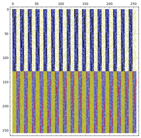
Figure 33: $[f_{8,10}]$: extended Cayley classes.

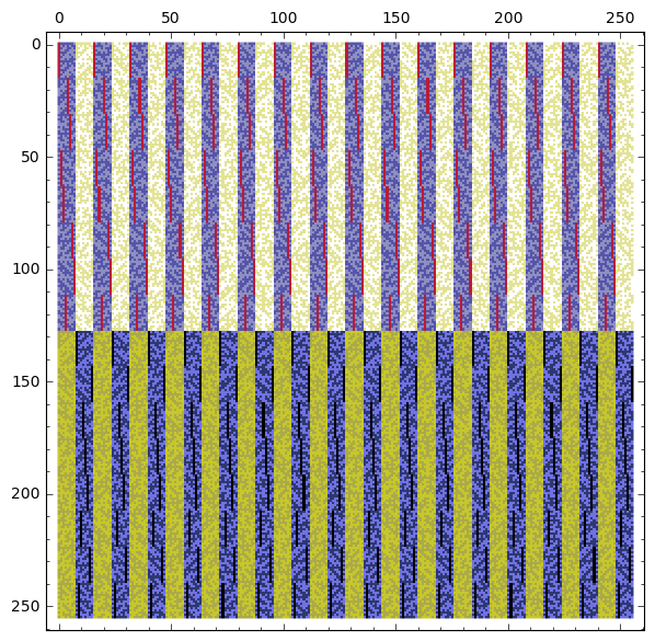
Figure 34: $[f_{8,10}]$: extended Cayley classes of dual bent functions.

B.5 Two sequences of bent functions

As stated in the introduction, in a recent paper [44], the author found an example of two infinite series of bent functions whose Cayley graphs have the same strongly regular parameters at each dimension, but are not isomorphic if the dimension is 8 or more. The sequences are $\sigma_{m}$ and $\tau_{m}$ for $m\geqslant 1$, whose definitions are reproduced here from [41].

Definition.

The sign-of-square function $\sigma_{m}:\mathbb{Z}_{2}^{2m}\rightarrow\mathbb{Z}_{2}$ is defined as follows:

For $i\in\mathbb{Z}_{2^{2m}},$ $\sigma_{m}(i)=1$ if and only if the number of 1 digits in the base 4 representation of $i$ is odd.

The non-diagonal-symmetry function $\tau_{m}\colon\mathbb{Z}_{2^{2m}}\rightarrow\mathbb{Z}_{2}$ is defined as follows.

For $i$ in $\mathbb{Z}_{2}^{2}$:

$$\tau_{1}(i):=\begin{cases}1&\text{if~{}}i=10,\\ 0&\text{otherwise}.\end{cases}$$

For $i$ in $\mathbb{Z}_{2}^{2m-2}$:

$$\tau_{m}(00\odot i):=\tau_{m-1}(i),$$

$$\tau_{m}(01\odot i):=\sigma_{m-1}(i),$$

$$\tau_{m}(10\odot i):=\sigma_{m-1}(i)+1,$$

$$\tau_{m}(11\odot i):=\tau_{m-1}(i).$$

where $\odot$ denotes concatenation of bit vectors, and $\sigma$ is the sign-of-square function, as above.

As shown in [41], both sequences produce Cayley graphs whose strongly regular parameters are

$$(v_{m},k_{m},\lambda_{m}=\mu_{m}) =(4^{m},2^{2m-1}-2^{m-1},2^{2m-2}-2^{m-1}).$$

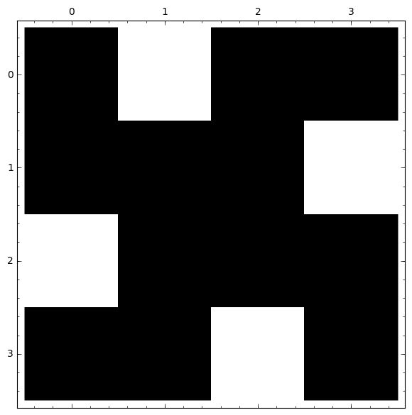
Figure 35: $[\sigma_{1}]$:
2 extended Cayley classes

Figure 36: $[\tau_{1}]$:
2 extended Cayley classes

Figure 37: $[\sigma_{2}]$:
2 extended Cayley classes

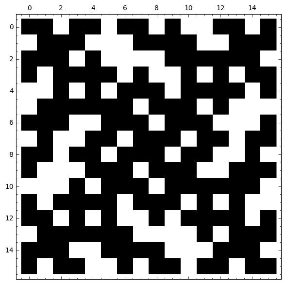
Figure 38: $[\tau_{2}]$:
2 extended Cayley classes

Figures 35 to 42 illustrate the extended Cayley classes within the ET classes of each of function $\sigma_{m}$ and $\tau_{m}$ for $m$ from 1 to 4. Note that $\tau_{3}$ has degree 3, and $\tau_{4}$ has degree 4. As shown in [44], The functions $\sigma_{m}$ and $\tau_{m}$ are extended Cayley equivalent for $m$ from 1 to 3, but are inequivalent for $m>3$.

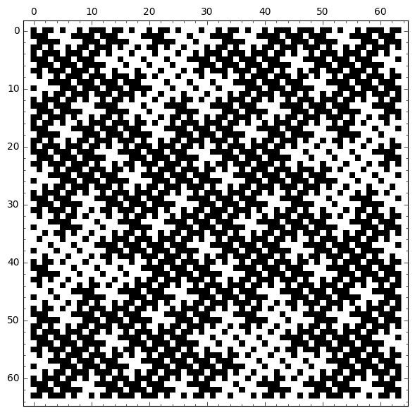
Figure 39: $[\sigma_{3}]$:
2 extended Cayley classes

Figure 40: $[\tau_{3}]$:
3 extended Cayley classes

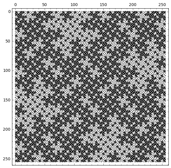
Figure 41: $[\sigma_{4}]$:
2 extended Cayley classes

Figure 42: $[\tau_{4}]$:
5 extended Cayley classes

B.6 CAST-128 S-boxes

The CAST-128 encryption algorithm is used in PGP and elsewhere [2]. The algorithm uses 8 S-boxes, each of which consists of 32 Boolean bent functions in 8 dimensions, with degree 4, making 256 bent functions in total. The full CAST-128 algorithm, including the contents of the S-boxes, is published as IETF Request For Comments 2144 [1].

The bent function $cast128_{1,0}$ is the first bent function of S-box number 1 of CAST-128. Its definition by algebraic normal form is

$$cast128_{1,0}:=\begin{array}[]{l}x_{0}x_{1}x_{2}x_{3}+x_{0}x_{1}x_{2}x_{4}+x_{0}x_{1}x_{2}x_{5}+x_{0}x_{1}x_{2}+x_{0}x_{1}x_{3}x_{5}+x_{0}x_{1}x_{3}x_{6}\,+\\ x_{0}x_{1}x_{3}+x_{0}x_{1}x_{5}x_{6}+x_{0}x_{1}x_{6}+x_{0}x_{1}x_{7}+x_{0}x_{2}x_{3}x_{4}+x_{0}x_{2}x_{3}\,+\\ x_{0}x_{2}x_{4}x_{5}+x_{0}x_{2}x_{5}x_{7}+x_{0}x_{2}x_{6}+x_{0}x_{2}x_{7}+x_{0}x_{2}+x_{0}x_{3}x_{4}x_{5}\,+\\ x_{0}x_{3}x_{4}x_{6}+x_{0}x_{3}x_{5}x_{6}+x_{0}x_{3}+x_{0}x_{4}x_{5}x_{6}+x_{0}x_{4}x_{5}x_{7}+x_{0}x_{4}x_{5}\,+\\ x_{0}x_{4}x_{6}+x_{0}x_{4}+x_{0}x_{5}x_{6}+x_{0}x_{5}x_{7}+x_{0}x_{6}+x_{0}x_{7}+x_{0}+x_{1}x_{2}x_{4}x_{6}\,+\\ x_{1}x_{2}x_{4}x_{7}+x_{1}x_{2}x_{5}x_{6}+x_{1}x_{2}x_{7}+x_{1}x_{3}x_{4}x_{6}+x_{1}x_{3}x_{4}x_{7}+x_{1}x_{3}x_{5}\,+\\ x_{1}x_{3}x_{7}+x_{1}x_{4}x_{5}x_{7}+x_{1}x_{4}x_{6}+x_{1}x_{5}x_{6}+x_{1}+x_{2}x_{3}x_{4}x_{6}+x_{2}x_{3}x_{4}\,+\\ x_{2}x_{3}x_{5}x_{6}+x_{2}x_{3}x_{5}+x_{2}x_{3}x_{7}+x_{2}x_{4}+x_{2}x_{5}x_{6}+x_{2}x_{5}+x_{2}+x_{3}x_{4}x_{5}x_{6}\,+\\ x_{3}x_{5}x_{6}+x_{3}x_{5}x_{7}+x_{3}x_{6}+x_{3}+x_{4}+x_{6}x_{7}.\end{array}$$

This bent function $cast128_{1,0}$ is prolific: the ET class $[cast128_{1,0}]$ contains the maximum possible number of Cayley classes, that is $65\,536$. The duals of the bent functions $[cast128_{1,0}]$ give another $65\,536$ extended Cayley classes. In other words, no bent function in $[cast128_{1,0}]$ is EA equivalent to its dual. The two weight classes of $[cast128_{1,0}]$ are shown in Figure 43.

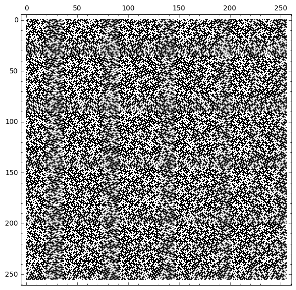
Figure 43: $[cast128_{1,0}]$:
Weight classes                
 
Colormap: gist_stern.

Figure 44: $[cast128_{1,0}]$:
$65\,536$ extended Cayley classes.
Total including duals is $131\,072$.
Colormap: jet.

Figure 45: $[cast128_{2,1}]$:
$8\,256$ extended Cayley classes.
Total including duals is $8\,256$.
Colormap: jet.

Figure 46: $[cast128_{2,16}]$:
$32\,768$ extended Cayley classes.
Total including duals is $65\,536$.
Colormap: jet.

Figure 47: $[cast128_{4,27}]$:
$65\,536$ extended Cayley classes.
Total including duals is $65\,536$.
Colormap: jet.

Figure 48: $[cast128_{5,16}]$:
$33\,280$ extended Cayley classes.
Total including duals is $66\,560$.
Colormap: jet.

Figure 49: $[cast128_{5,27}]$:
$6\,144$ extended Cayley classes.
Total including duals is $6\,144$.
Colormap: jet.

Figure 50: $[cast128_{6,17}]$:
$65\,536$ extended Cayley classes.
Total including duals is $65\,536$.
Colormap: jet.

Figure 51: $[cast128_{7,15}]$:
$32\,768$ extended Cayley classes.
Total including duals is $65\,536$.
Colormap: jet.

Figure 52: $[cast128_{7,21}]$:
$32\,768$ extended Cayley classes.
Total including duals is $65\,536$.
Colormap: jet.

Of the 256 bent functions that make up the 8 S-boxes of CAST-128, 248 are like $cast128_{1,0}$, they are prolific and are not EA equivalent to their duals. The remaining 8 bent functions are exceptional. Both $cast128_{4,27}$ and $cast128_{6,17}$ are prolific, but both are EA equivalent to their duals.

The other 6 bent functions are not prolific and the number of Cayley classes for each is given in the captions to Figures 45 to 52.

B.7 Partial spread bent functions.

According to Langevin and Hou [36] there are $70\,576\,747\,237\,594\,114\,392\,064\approx 2^{75.9}$ partial spread bent functions in dimension 8, contained in $14\,758$ EA classes. The EA class representatives are listed at Langevin’s web page [35]. On this web page, the file psf-8.txt contains details of $9316$ representatives that are $\mathcal{PS}^{(-)}$ bent functions, all of degree 4; and the file psf-9.txt contains details of $5442$ representatives that are $\mathcal{PS}^{(+)}$ bent functions, of which $5440$ are of degree 4.

Preliminary calculations using SageMath on the NCI Raijin supercomputer indicate that

1. The $5442$ EA classes of $\mathcal{PS}^{(+)}$ bent functions of dimension 8 contain $296\,594\,720$ extended Cayley classes, assuming that each extended Cayley class appears in only one of the EA classes.

2. If the duals of the $5442$ representatives, and their corresponding EA classes are included, the total number of extended Cayley classes is $541\,700\,450$, under the same assumption.

3. Of the $5442$ representatives, $3434$ are prolific and not EA equivalent to their dual, $582$ are prolific and are EA equivalent to their dual, and the EA classes of the remaining $1426$ each contain less than $65\,536$ extended Cayley classes.

The classifications of these $5442$ EA classes take up $2.1\,$TB of space on the NCI Raijin supercomputer. The classifications of the $9316$ $\mathcal{PS}^{(-)}$ bent functions are currently being generated on Raijin. In total, the classifications of the $\mathcal{PS}^{(+)}$ and $\mathcal{PS}^{(-)}$ bent functions are estimated to take up $6\,$TB of space on Raijin. It is intended that these classifications will be incorporated into a public database, if support can be found to maintain it [40].

One example classification from $\mathcal{PS}^{(+)}$ in dimension 8 is that of $psf_{9,5439}$. The bent function $psf_{9,5439}$ is listed as function number $5439$ in psf-9.txt, and is a $\mathcal{PS}^{(+)}$ bent function of degree 4. Its ET class $[psf_{9,5439}]$ contains 16 extended Cayley classes, of which 6 form three duality pairs similar to those seen in $[f_{8,9}]$ and $[f_{8,10}]$ above.

The 16 extended Cayley classes are distributed as shown in Figures 53 (classes) and 54 (classes of duals).

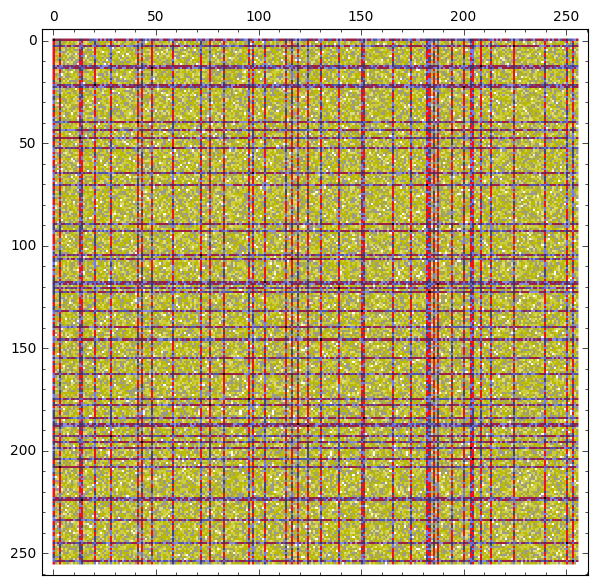
Figure 53: $[psf_{9,5439}]$:
extended Cayley classes             
         

Figure 54: $[psf_{9,5439}]$:
extended Cayley classes of dual bent
functions

References

• [1] C. M. Adams. The CAST-128 encryption algorithm. RFC 2144, RFC Editor, May 1997.
• [2] C. M. Adams. Constructing symmetric ciphers using the CAST design procedure. In E. Kranakis and P. Van Oorschot, editors, Selected Areas in Cryptography, 71–104, Boston, MA, (1997). Springer US.
• [3] A. Bernasconi and B. Codenotti. Spectral analysis of Boolean functions as a graph eigenvalue problem. IEEE Transactions on Computers, 48(3):345–351, (1999).
• [4] A. Bernasconi, B. Codenotti, and J. M. VanderKam. A characterization of bent functions in terms of strongly regular graphs. IEEE Transactions on Computers, 50(9):984–985, (2001).
• [5] J. Borwein and K. Devlin. The computer as crucible: An introduction to experimental mathematics. AK Peters/CRC Press, (2008).
• [6] R. C. Bose. Strongly regular graphs, partial geometries and partially balanced designs. Pacific J. Math, 13(2):389–419, (1963).
• [7] I. Bouyukliev, V. Fack, W. Willems, and J. Winne. Projective two-weight codes with small parameters and their corresponding graphs. Designs, Codes and Cryptography, 41(1):59–78, (2006).
• [8] A. Braeken. Cryptographic Properties of Boolean Functions and S-Boxes. PhD thesis, Katholieke Universiteit Leuven, Leuven-Heverlee, Belgium, (2006).
• [9] A. Brouwer, A. Cohen, and A. Neumaier. Distance-Regular Graphs. Ergebnisse der Mathematik und Ihrer Grenzgebiete, 3 Folge / A Series of Modern Surveys in Mathematics. Springer London, (2011).
• [10] A. E. Brouwer and C. A. Van Eijl. On the p-rank of the adjacency matrices of strongly regular graphs. Journal of Algebraic Combinatorics, 1(4):329–346, (1992).
• [11] R. Calderbank and W. M. Kantor. The geometry of two-weight codes. Bulletin of the London Mathematical Society, 18(2):97–122, (1986).
• [12] P. J. Cameron. Random strongly regular graphs? Discrete Mathematics, 273(1):103–114, (2003). EuroComb’01.
• [13] P. J. Cameron and J. H. Van Lint. Designs, graphs, codes and their links, volume 3. Cambridge University Press, (1991).
• [14] C. Carlet. Boolean functions for cryptography and error correcting codes. In Boolean Models and Methods in Mathematics, Computer Science, and Engineering, volume 2, 257–397. Cambridge University Press, (2010).
• [15] C. Carlet, L. E. Danielsen, M. G. Parker, and P. Solé. Self-dual bent functions. International Journal of Information and Coding Theory, 1(4):384–399, (2010).
• [16] C. Carlet and S. Mesnager. Four decades of research on bent functions. Designs, Codes and Cryptography, 78(1):5–50, (2016).
• [17] Y. M. Chee, Y. Tan, and X. D. Zhang. Strongly regular graphs constructed from p-ary bent functions. Journal of Algebraic Combinatorics, 34(2):251–266, (2011).
• [18] J. D. Comerford. Affine and general linear equivalences of Boolean functions. Information and Control, 45(2):156–169, (1980).
• [19] T. W. Cusick and P. Stanica. Cryptographic Boolean functions and applications. Academic Press, 2nd edition, (2017).
• [20] P. Delsarte. Weights of linear codes and strongly regular normed spaces. Discrete Mathematics, 3(1-3):47–64, (1972).
• [21] J. F. Dillon. Elementary Hadamard Difference Sets. PhD thesis, University of Maryland College Park, Ann Arbor, USA, (1974).
• [22] J. F. Dillon and J. R. Schatz. Block designs with the symmetric difference property. In Proceedings of the NSA Mathematical Sciences Meetings, 159–164. US Govt. Printing Office Washington, DC, (1987).
• [23] C. Ding. Linear codes from some 2-designs. IEEE Transactions on information theory, 61(6):3265–3275, (2015).
• [24] C. Ding, S. Mesnager, C. Tang, and M. Xiong. Cyclic bent functions and their applications in codes, codebooks, designs, MUBs and sequences. arXiv preprint arXiv:1811.07725, (2018).
• [25] T. Feulner, L. Sok, P. Solé, and A. Wassermann. Towards the classification of self-dual bent functions in eight variables. Designs, Codes and Cryptography, 68(1):395–406, (2013).
• [26] M. A. Harrison. On the classification of Boolean functions by the general linear and affine groups. Journal of the Society for Industrial and Applied Mathematics, 12(2):285–299, (1964).
• [27] C. Hoede and X. Li. Clique polynomials and independent set polynomials of graphs. Discrete Mathematics, 125(1):219 – 228, (1994).
• [28] T. Huang and K.-H. You. Strongly regular graphs associated with bent functions. In 7th International Symposium on Parallel Architectures, Algorithms and Networks, 2004. Proceedings., 380–383, May 2004.
• [29] N. Jacobson. Lectures in Abstract Algebra: III. Theory of Fields and Galois Theory (Graduate Texts in Mathematics). Van Nostrand, (1964).
• [30] D. Joyner, O. Geil, C. Thomsen, C. Munuera, I. Márquez-Corbella, E. Martínez-Moro, M. Bras-Amorós, R. Jurrius, and R. Pellikaan. Sage: A basic overview for coding theory and cryptography. In Algebraic Geometry Modeling in Information Theory, volume 8 of Series on Coding Theory and Cryptology, 1–45. World Scientific Publishing Company, (2013).
• [31] T. Junttila and P. Kaski. Engineering an efficient canonical labeling tool for large and sparse graphs. In D. Applegate, G. S. Brodal, D. Panario, and R. Sedgewick, editors, Proceedings of the Ninth Workshop on Algorithm Engineering and Experiments and the Fourth Workshop on Analytic Algorithms and Combinatorics, 135–149, New Orleans, LA, (2007). Society for Industrial and Applied Mathematics.
• [32] T. Junttila and P. Kaski. Conflict propagation and component recursion for canonical labeling. In Theory and Practice of Algorithms in (Computer) Systems, 151–162. Springer, (2011).
• [33] W. M. Kantor. Symplectic groups, symmetric designs, and line ovals. Journal of Algebra, 33(1):43–58, (1975).
• [34] W. M. Kantor. Exponential numbers of two-weight codes, difference sets and symmetric designs. Discrete Mathematics, 46(1):95–98, (1983).
• [35] P. Langevin. Classification of partial spread functions in eight variables, (2010). http://langevin.univ-tln.fr/project/spread/psp.html.
• [36] P. Langevin and X.-D. Hou. Counting partial spread functions in eight variables. IEEE Transactions on Information Theory, 57(4):2263–2269, (2011).
• [37] P. Langevin and G. Leander. Counting all bent functions in dimension eight 99270589265934370305785861242880. Designs, Codes and Cryptography, 59(1-3):193–205, (2011).
• [38] P. Langevin, G. Leander, and G. McGuire. Kasami bent functions are not equivalent to their duals. In G. Mullen, D. Panario, and I. Shparlinski, editors, Finite Fields and Applications: Eighth International Conference on Finite Fields and Applications, July 9-13, 2007, Melbourne, Australia, 187–198. American Mathematical Society, (2008).
• [39] A. Lempel. Matrix factorization over gf(2) and trace-orthogonal bases of gf(2^n). SIAM Journal on Computing, 4(2):175–186, (1975).
• [40] P. Leopardi. A database of Cayley graphs of bent Boolean functions. In preparation.
• [41] P. Leopardi. Twin bent functions and Clifford algebras. In Algebraic Design Theory and Hadamard Matrices, 189–199. Springer, (2015).
• [42] P. Leopardi. Boolean-cayley-graphs, (2016). https://github.com/penguian/Boolean-Cayley-graphs GitHub repository.
• [43] P. Leopardi. Boolean-cayley-graphs, (2017). http://tinyurl.com/Boolean-Cayley-graphs CoCalc public folder.
• [44] P. Leopardi. Twin bent functions, strongly regular Cayley graphs, and Hurwitz-Radon theory. Journal of Algebra Combinatorics Discrete Structures and Applications, 4(3):271–280, (2017).
• [45] F. J. MacWilliams and N. J. A. Sloane. The theory of error-correcting codes. Elsevier, (1977).
• [46] J. A. Maiorana. A classification of the cosets of the Reed-Muller code R(1, 6). Mathematics of Computation, 57(195):403–414, (1991).
• [47] B. D. McKay and A. Piperno. Nauty and Traces user’s guide (Version 2.5). Computer Science Department, Australian National University, Canberra, Australia, (2013).
• [48] B. D. McKay and A. Piperno. Practical graph isomorphism, II. Journal of Symbolic Computation, 60:94–112, (2014).
• [49] W. Meier and O. Staffelbach. Nonlinearity criteria for cryptographic functions. In J.-J. Quisquater and J. Vandewalle, editors, Advances in Cryptology — EUROCRYPT ’89: Workshop on the Theory and Application of Cryptographic Techniques, volume 434 of Lecture Notes in Computer Science, 549–562, Berlin, Heidelberg, (1990). Springer.
• [50] S. Mesnager. Bent functions. Springer, (2016).
• [51] D. E. Muller. Application of Boolean algebra to switching circuit design and to error detection. Transactions of the IRE Professional Group on Electronic Computers, (3):6–12, (1954).
• [52] T. Neumann. Bent functions. PhD thesis, University of Kaiserslautern, (2006).
• [53] J. Olsen, R. Scholtz, and L. Welch. Bent-function sequences. IEEE Transactions on Information Theory, 28(6):858–864, November 1982.
• [54] PostgreSQL Global Development Group. PostgreSQL, (1996). https://www.postgresql.org.
• [55] O. S. Rothaus. On “bent” functions. Journal of Combinatorial Theory, Series A, 20(3):300–305, (1976).
• [56] G. F. Royle. A normal non-cayley-invariant graph for the elementary abelian group of order 64. Journal of the Australian Mathematical Society, 85(03):347–351, (2008).
• [57] R. Rueppel. Analysis and design of stream ciphers. Communications and control engineering series. Springer, (1986).
• [58] SageMath, Inc. CoCalc - Collaborative Calculation in the Cloud, (2017). https://cocalc.com/.
• [59] J. J. Seidel. Strongly regular graphs. In Surveys in combinatorics (Proc. Seventh British Combinatorial Conf., Cambridge, 1979), volume 38 of London Mathematical Society Lecture Note Series, 157–180, Cambridge-New York, (1979). Cambridge Univ. Press.
• [60] SQLite Consortium. SQLite, (2000). http://sqlite.org.
• [61] P. Stanica. Graph eigenvalues and Walsh spectrum of Boolean functions. Integers: Electronic Journal Of Combinatorial Number Theory, 7(2):A32, (2007).
• [62] D. R. Stinson. Combinatorial designs: constructions and analysis. Springer Science & Business Media, (2007).
• [63] The Sage Developers. SageMath, the Sage Mathematics Software System (Version 7.5), (2017). http://www.sagemath.org.
• [64] The Sage Developers. SageMath, the Sage Mathematics Software System (Version 8.4), (2018). http://www.sagemath.org.
• [65] N. Tokareva. Bent functions: results and applications to cryptography. Academic Press, (2015).
• [66] V. D. Tonchev. The uniformly packed binary [27, 21, 3] and [35, 29, 3] codes. Discrete Mathematics, 149(1-3):283–288, (1996).
• [67] V. D. Tonchev. Codes. In C. Colbourne and J. Dinitz, editors, Handbook of combinatorial designs, chapter VII.1, 677–701. CRC press, second edition, (2007).