Persistence of the flat band in a kagomé magnet with dipolar interactions

Abstract

The weathervane modes of the classical Heisenberg antiferromagnet on the kagomé lattice constitute possibly the earliest and certainly the most celebrated example of a flat band of zero-energy excitations. Such modes arise from the underconstraint that has since become a defining criterion of strong geometrical frustration. We investigate the fate of this flat band when dipolar interactions are added. These change the nearest-neighbour model fundamentally as they remove the Heisenberg spin-rotational symmetry while also introducing a long-range component to the interaction. We explain how the modes continue to remain approximately dispersionless, while being lifted to finite energy as well as being squeezed: they change their ellipticity described by the ratio of the amplitudes of the canonically conjugate variables comprising them. This phenomenon provides interesting connections between concepts such as constraint counting and self-screening underpinning the field of frustrated magnetism. We discuss variants of these phenomena for different interactions, lattices and dimension.

I Introduction

One of the hallmarks of geometrical frustration in classical spin models is a large ground-state degeneracy associated with their ground states. For discrete Ising spins, this leads to a non-vanishing ‘ground-state entropy’ such as Pauling’s entropy in spin ice Ramirez et al. (1999), for a review see Castelnovo et al. (2012). For continuous spins, the ground states form a manifold of extensive dimensionality Moessner and Chalker (1998a, b). Continuous rearrangements of spins effecting moves between these degenerate ground-state configurations form zero-energy modes of the system.

If such zero-energy modes are local, i.e. involve only a finite number of spins, they are often referred to as weathervane modesChalker et al. (1992); Ritchey et al. (1993); Shender et al. (1993). Their locality implies a straightforward possibility of a non-zero density of them, and hence an extensive number resulting in the existence of a flat zero-energy band in momentum space. A typical scenario for the appearance of such modes in classical spin models is provided by the locally underconstrained nature of the spin interactions, whereby a mismatch between the number of degrees of freedom and the number of ground state constraints imposed by the Hamiltonian is extensive Moessner and Chalker (1998a, b). As such, the existence of these local modes is not protected by any symmetries and can be easily destroyed by perturbations – e.g. next-nearest neighbour interactions – which typically increase the number of constraints, rendering the formerly flat zero-energy bands dispersive Harris et al. (1992). When such additional interactions also break the symmetries of the Hamiltonian, even gaplessness of the spectrum is no longer guaranteed and interesting phenomenon can arise: the formerly flat zero-energy bands can be lifted up to finite energy but remain flat Chernyshev and Zhitomirsky (2015). One example of such behaviour has been recently observed in the kagomé Heisenberg antiferromagnet (KHAFM) with an additional out-of-plane Dzyaloshinskii-Moriya (DM) interaction (albeit in this case another magnon band remained gapless due to the remaining U(1) symmetry of the Hamiltonian). The persisting flatness of such a band implies the local nature of the spin excitations; in other words such excitations preserve their weathervane character.

Many recent discussions have been centred around flat bands in fermionic systems due to the fact that, if partially occupied, they provide a fertile ground for a variety of unconventional orders (for reviews, see e.g. Ref. Parameswaran et al., 2013; Bergholtz and Liu, 2013; Derzhko et al., 2015). More exotic flavours and settings–e.g. lattices for which all bands are flat Vidal et al. (1998), lattices with ‘higher-spin’ Weyl fermions Dóra et al. (2011), or in the currently very fashionable Floquet setting Du et al. (2017) – have also been considered over the years. Even when not hosting any exotic topological orders, such bands can nevertheless be responsible for unusual thermodynamic, dynamic and transport properties. These properties need not be restricted to fermionic flat bands; their bosonic counterparts can be responsible for a variety of interesting phenomena such as magnetisation plateaux in frustrated magnets at high magnetic fields Schulenburg et al. (2002); Zhitomirsky and Tsunetsugu (2005); Schmidt et al. (2006); Derzhko et al. (2007).

In this work we report a simple example of a system hosting a flat magnon band in the absence of any external field: a large-spin KHAFM with additional dipolar spin–spin interaction. The dipolar interaction breaks the SU(2) symmetry of the Heisenberg Hamiltonian down to $\mathbb{Z}_{2}\times\mathbb{Z}_{2}$, the largest subgroup consistent with the point group symmetry of the kagomé lattice, and hence (unsurprisingly) completely gaps the magnon spectrum. What is surprising is that the lowest excitation band stays perfectly flat in the case of truncated nearest-neighbour dipolar interactions and remains flat to a very good approximation for the complete long-range case. The energy of the flat band is proportional to $\sqrt{\gamma}$, where $\gamma$ is the strength of the dipolar term. While in the case of constraint counting for the nearest-neighbour KHAFM, the flatness simply follows from the fact that the modes are pinned to zero energy, its origin here is considerably less transparent.

Our central result is that the survival of flatness rests on two ingredients. The first is that the canonical structure of the flat modes comprises a pair of conjugate variables, both of which have a flat momentum dependence, so that they can combine into a flat band at finite frequency. This double flatness is a very peculiar feature of the kagomé magnet which, to the best of our knowledge, has not yet been explicitly identified. As the magnitude of the dipolar term is increased, the ellipticity of the mode changes from 0 for the Heisenberg weathervane mode to a finite value, reminiscent to the physics of squeezing in quantum optics, but with a concomitant change in frequency for the modes here.

For the case of truncated dipolar interactions with their range limited to the nearest neighbours, we present an exact analytical calculation illuminating the microscopic nature of the modes comprising the flat band. The survival of the flatness for the full long-range dipolar interaction requires the second ingredient: both conjugate variables encode a mode with vanishing net spin moment. This renders the long-range (inverse cube) tails of the dipolar interaction ineffective for this particular type of spin excitations, the long corrections are dominated by shorter range, higher terms in the multipole expansion. This is analogous to the phenomenon of self-screening first noticed for Ising spins in the context of dipolar spin iceden Hertog and Gingras (2000) and later explained in terms of a projective equivalenceIsakov et al. (2005), with a simple picture provided by a dumbbell model for the Ising spins Castelnovo et al. (2008); our model provides an example of such a behaviour for continuous spins.

Furthermore, we show that the presence of a flat spin wave mode is a rather generic feature of a large spin kagomé antiferromagnet. This effect is found to survive the addition of other interaction terms such as the Dzyaloshinskii–Moriya or anisotropic terms (consistent with the symmetries of the kagomé lattice) within an extended range of parameters.

We note that finite frequency flat bands have been experimentally observed in other frustrated spin systems with dipolar interactions, such as gadolinium gallium garnet d’Ambrumenil et al. (2015); the physics described here need not be limited to the kagomé lattice.

II 2D kagomé Heisenberg antiferromagnet

In this section we briefly review some known results for the classical KHAFM. The Heisenberg Hamiltonian can be written as

$$H_{\text{KHAFM}}=J\sum_{\langle i,j\rangle}\mathbf{S}_{i}\cdot\mathbf{S}_{j}=\frac{J}{2}\sum_{\vartriangle}\mathbf{S_{\vartriangle}}^{2}+\text{const}$$ (1)

where the second sum is performed over all triangles of the kagomé lattice and $\mathbf{S_{\vartriangle}}$ is the combined spin of the three sites forming a given triangle. The energy is minimised by a state with all $\mathbf{S_{\vartriangle}}=0$, implying that any $120^{\circ}$ arrangement of spins around every triangle corresponds to a classical ground state of this Hamiltonian.

The ground state manifold has an extensive dimensionality. One of the key results of the early spin-wave analyses of this model is that a co-planar subset of this manifold is selected by the order-by-disorder mechanism Chalker et al. (1992); Harris et al. (1992); Huse and Rutenberg (1992); Ritchey et al. (1993). The two most prominent types of these states, the $q=0$ and $\sqrt{3}\times\!\sqrt{3}$ states, are shown here in Figure 1. In linear spin-wave theory, the spectra of all coplanar states are identicalChalker et al. (1992), a feature not present in the full nonlinear problem Chubukov (1992); von Delft and Henley (1992); Chern and Moessner (2013).

The $\sqrt{3}\times\!\sqrt{3}$ state, shown in Figure 1, serves as an archetypal example of a state supporting an exact local zero energy mode – a.k.a.  weathervane mode – which corresponds to rotations of e.g. A- and B-spins located around a single hexagon of the lattice around the axis given by the direction of the C-spins. Nevertheless all co-planar ground states posses such soft modes in the harmonic approximation, and hence are characterised by a zero-energy magnon band.

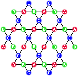
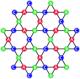
Figure 1: (Colour online) Ground states of the KHAFM: (a) the $q=0$ state; (b) the $\sqrt{3}\times\!\sqrt{3}$ state. A, B and C here label three directions of spins in a $120^{\circ}$ configuration: $\mathbf{S}_{\text{A}}+\mathbf{S}_{\text{B}}+\mathbf{S}_{\text{C}}=0$.

III Adding dipolar interactions

We now extend the KHAFM model (1) by adding magnetic dipolar interations between spins:

$$H_{\text{KH+D}}=J\sum_{\langle i,j\rangle}\mathbf{S}_{i}\cdot\mathbf{S}_{j}+\frac{1}{2}\sum_{i,j}\gamma_{ij}^{\alpha\beta}S_{i}^{\alpha}S_{j}^{\beta}$$ (2)

where the second sum is not restricted to nearest neighbours and

$$\gamma_{ij}^{\alpha\beta}=\gamma a^{3}\left(\frac{\delta_{\alpha\beta}}{\lvert{\mathbf{r}_{ij}}\rvert^{3}}-3\frac{{r}_{ij}^{\alpha}{r}_{ij}^{\beta}}{\lvert{\mathbf{r}_{ij}}\rvert^{5}}\right).$$ (3)

Here $a$ is the lattice constant, $\mathbf{r}_{ij}\equiv\mathbf{r}_{j}-\mathbf{r}_{i}$ and $\gamma=g^{2}\mu_{\text{B}}^{2}/a^{3}$ (in Gaussian units).

Remarkably, in the presence of a relatively small Heisenberg term, this dipolar term does not compete with the nearest-neighbour exchange: the ground state is still one the of $120^{\circ}$ states. More specifically, the ground state, shown here in Figure 2, is one of the $q=0$ states (see Figure 1). The spins at each site align in the direction parallel to that of the opposite side of a triangle this spin belongs to, with the three spins around each triangle adding to 0. This ground state is doubly degenerate, with respect to a global reversal of all spins.

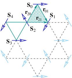
Figure 2: (Colour online) One of the two classical ground states of the KHAFM with the additional dipolar interactions between spins.

Note that the $120^{{}^{\circ}}$ state is not a ground state of the long-range dipolar Hamiltonian alone Maksymenko et al. (2015). However, it is easy to verify its local extremality. Let us first consider the case of dipolar interactions whose range is restricted only to the nearest neighbours. The Hamiltonian is

$$H_{\text{KH+NND}}=\sum_{\langle i,j\rangle}\big{\{}(J+\gamma)\mathbf{S}_{i}\cdot\mathbf{S}_{j}\\ -3\gamma\left(\mathbf{S}_{i}\cdot\hat{\mathbf{r}}_{ij}\right)\left(\mathbf{S}_{j}\cdot\hat{\mathbf{r}}_{ij}\right)\big{\}},$$ (4)

where $\hat{\mathbf{r}}_{ij}$ is the unit vector directed from site $i$ to site $j$. In order to analyse the ground state of this Hamiltonian, let us focus on just two of its terms, specifically those involving interactions between spin $\mathbf{S}_{0}$ and two of its neighbours, $\mathbf{S}_{1}$ and $\mathbf{S}_{2}$, shown in Figure 2. These terms can be rewritten as

$$H_{01}+H_{02}\\ =\big{\{}(J+\gamma)\mathbf{S}_{0}\cdot\mathbf{S}_{1}-3\gamma\left(\mathbf{S}_{0}\cdot\hat{\mathbf{r}}_{01}\right)\left(\mathbf{S}_{1}\cdot\hat{\mathbf{r}}_{01}\right)\big{\}}\\ +\big{\{}(J+\gamma)\mathbf{S}_{0}\cdot\mathbf{S}_{2}-3\gamma\left(\mathbf{S}_{0}\cdot\hat{\mathbf{r}}_{20}\right)\left(\mathbf{S}_{2}\cdot\hat{\mathbf{r}}_{20}\right)\big{\}}\\ =-\mathbf{\tilde{h}}_{0}\cdot\mathbf{S}_{0},$$ (5)

where

$$\mathbf{\tilde{h}}_{0}=-(J+\gamma)\left(\mathbf{S}_{1}+\mathbf{S}_{2}\right)\\ +3\gamma\left[\hat{\mathbf{r}}_{01}\left(\mathbf{S}_{1}\cdot\hat{\mathbf{r}}_{01}\right)+\hat{\mathbf{r}}_{20}\left(\mathbf{S}_{2}\cdot\hat{\mathbf{r}}_{20}\right)\right]\\ =\hat{\mathbf{r}}_{21}\left(J+5\gamma/2\right)S.$$ (6)

In deriving the last line we used the fact that in the state shown in Figure 2, $\mathbf{S}_{1}+\mathbf{S}_{2}=-\mathbf{S}_{0}=-S\hat{\mathbf{r}}_{21}$ and $\mathbf{S}_{1}\cdot\hat{\mathbf{r}}_{01}=\mathbf{S}_{2}\cdot\hat{\mathbf{r}}_{20}=S/2$ as well as $\hat{\mathbf{r}}_{20}+\hat{\mathbf{r}}_{01}=\hat{\mathbf{r}}_{21}$. In other words, spin $\mathbf{S}_{0}$ is aligned with the effective magnetic field due to its neighbours (the effective field is actually $\mathbf{h}_{0}=2\mathbf{\tilde{h}}_{0}$ since another $\mathbf{\tilde{h}}_{0}$ results from $\mathbf{S}_{0}$’s two other neighbours).

Next, consider the following two observations. Firstly, accounting for longer-range dipolar interactions does not tilt $\mathbf{h}_{0}$ away from the horizontal, albeit can potentially reverse its direction (thus making this equilibrium state unstable). In order to see this, consider a pair of spins situated on the same horizontal line at sites which are symmetric with respect to the vertical line passing through the location of $\mathbf{S}_{0}$ (see Figure 2). Using the fact that this state is a $q=0$ state shown in Figure 1, we know that either both of the spins are of type C (i.e., the same as $\mathbf{S}_{0}$) or one of them is of type A while the other one is of type B. Denoting these sites as $k$ and $l$, we note that either $\mathbf{S}_{k}+\mathbf{S}_{l}=2\mathbf{S}_{0}$ (if both $\mathbf{S}_{k}$ and $\mathbf{S}_{l}$ are of type C) or else $\mathbf{S}_{k}+\mathbf{S}_{l}=-\mathbf{S}_{0}$. Meantime $\mathbf{S}_{k}\cdot\hat{\mathbf{r}}_{0k}=\mathbf{S}_{l}\cdot\hat{\mathbf{r}}_{l0}$ while $\hat{\mathbf{r}}_{l0}+\hat{\mathbf{r}}_{0k}\propto\hat{\mathbf{r}}_{lk}$. In other words, the contribution of the pair of spins at sites $k$ and $l$ into the effective field acting on $\mathbf{S}_{0}$ is still collinear with the direction of $\mathbf{S}_{0}$ albeit its sign depends on the location of the pair. As a result, the net effective field due to all spins interacting with $\mathbf{S}_{0}$ via untruncated dipolar coupling need not be positive. In fact, that is exactly what happens, and the state shown in Figure 2 is not a ground state of long-range dipolar Hamiltonian alone Maksymenko et al. (2015). However, a small nearest-neighbour Heisenberg term $J\gtrsim 0.1\gamma$ (which is already accounted for in Eq. (6)) will align $\mathbf{h_{0}}$ with $\mathbf{S}_{0}$ and stabilise this ground state Maksymenko et al. (2015).

Appendix A presents a different way of writing the Hamiltonian for the nearest neighbour Heisenberg and dipolar interactions which is useful in analysing the stability of the aforementioned ground state in the presence of some other interactions, such as the Dzyaloshinskii–Moriya interaction.

The stability analysis presented here is also a useful departing point for understanding the nature of the flat spin-wave band in this system. In particular, it allows for an identification of a local mode in the case of nearest-neighbour dipolar interactions. Specifically, we note that according to Eq. (6), the direction of the “restoring field” $\mathbf{h}_{0}$ acting on $\mathbf{S}_{0}$ due to the two neighbouring spins, $\mathbf{S}_{1}$ and $\mathbf{S}_{2}$, remains unchanged if these two spins tilt away from their equilibrium positions by the same angle in opposite directions. This is because $\mathbf{S}_{1}+\mathbf{S}_{2}$ remains parallel to $\hat{\mathbf{r}}_{21}$ while $\mathbf{S}_{2}\cdot\hat{\mathbf{r}}_{20}=\mathbf{S}_{1}\cdot\hat{\mathbf{r}}_{01}$ . Therefore, spin $\mathbf{S}_{0}$ experiences no torque and maintains its orientation. Moreover, if all six spins around a given hexagon (e.g. $\mathbf{S}_{1}$, $\mathbf{S}_{2}$, $\mathbf{S}_{3}\ldots$ in Fig. 2) rotate by the same amounts in alternating directions, none of the surrounding spins (i.e. $\mathbf{S}_{0}$, $\mathbf{S}_{4}\ldots$ in Fig. 2) would experience any torque as a result of such a vibrational mode – i.e., the mode will remain local.

In the next section we provide a semiclassical treatment of such a mode to show that it is indeed an eigenmode of the Hamiltonian (4) and evaluate its frequency.

IV The weathervane mode

Having identified the nature of the local mode, we now proceed with the semiclassical equations of motions for the affected spins. To that end, we shall focus on spin $\mathbf{S}_{2}$. Provided that all terms in the Hamiltonian containing $\mathbf{S}_{2}$ can be combined together so that $H_{2}=-\mathbf{h}_{2}\cdot\mathbf{S}_{2}$, the EOM for this spin is given by

$$\hbar\frac{d\mathbf{S}_{2}}{dt}=\mathbf{S}_{2}\times\mathbf{h}_{2},$$ (7)

which is simply the Landau–Lifshitz equation. Here $\mathbf{h}_{2}$ is the effective field due to the interaction of $\mathbf{S}_{2}$ with four neighbouring spins; we can readily use Eq. (6) to write

$$\mathbf{h}_{2}=-(J+\gamma)\left(\mathbf{S}_{0}+\mathbf{S}_{1}+\mathbf{S}_{3}+\mathbf{S}_{4}\right)\\ +3\gamma\left[\hat{\mathbf{r}}_{20}\left(\mathbf{S}_{0}\cdot\hat{\mathbf{r}}_{20}\right)+\hat{\mathbf{r}}_{21}\left(\mathbf{S}_{1}\cdot\hat{\mathbf{r}}_{21}\right)\right.\\ \left.+\hat{\mathbf{r}}_{23}\left(\mathbf{S}_{3}\cdot\hat{\mathbf{r}}_{23}\right)+\hat{\mathbf{r}}_{24}\left(\mathbf{S}_{4}\cdot\hat{\mathbf{r}}_{24}\right)\right].$$ (8)

Using the fact that spins $\mathbf{S}_{0}$ and $\mathbf{S}_{4}$ keep their ground state orientation, we can simplify this equation to read

$$\mathbf{h}_{2}=-\left(J+{5}\gamma/2\right)S\hat{\mathbf{r}}_{01}-(J+\gamma)\left(\mathbf{S}_{1}+\mathbf{S}_{3}\right)\\ +3\gamma\left[\hat{\mathbf{r}}_{21}\left(\mathbf{S}_{1}\cdot\hat{\mathbf{r}}_{21}\right)+\hat{\mathbf{r}}_{23}\left(\mathbf{S}_{3}\cdot\hat{\mathbf{r}}_{23}\right)\right].$$ (9)

Let us choose local right-handed coordinate systems so that the $z$-axis at each site points along the equilibrium direction of its spin while all $x$-axes point out of the plane (towards the reader). Recall that in the putative local weathervane mode, spins $\mathbf{S}_{1}$ and $\mathbf{S}_{3}$ tilt away from their equilibrium positions by the same amount. Thus the respective components of $\mathbf{S}_{1}$ and $\mathbf{S}_{3}$ are equal to one another, $S_{1}^{\alpha}=S_{3}^{\alpha}$ (which, of course does not imply that $\mathbf{S}_{1}=\mathbf{S}_{3}$ since the local axes are different at these sites!). We can then write the effective field at the location of $\mathbf{S}_{2}$ as

$$\mathbf{h}_{2}=\left(\!-2\left(J\!+\!\gamma\right)\!S^{x}_{1},\left(\!J\!-\!\frac{7\gamma}{2}\!\right)\!S^{y}_{1},\left(\!J+\frac{5}{2}\gamma\!\right)\left(S^{z}_{1}+S\right)\!\right)$$

and the resulting linearised EOMs then become

$$\hbar\frac{dS^{x}_{2}}{dt}\approx S\left(\left(5\gamma+2J\right)S^{y}_{2}-\left(J-\frac{7}{2}\gamma\right)S^{y}_{1}\right)$$ (10a)

$$\hbar\frac{dS^{y}_{2}}{dt}\approx S\left(-2\left(J+\gamma\right)S^{x}_{1}-\left(2J+5\gamma\right)S^{x}_{2}\right),$$ (10b)

$$\hbar\frac{dS^{z}_{2}}{dt}=S^{x}_{2}h^{y}-S^{y}_{2}h^{x}=\mathcal{O}({S^{x}}^{2},{S^{y}}^{2})\approx 0,$$ (10c)

where we used the fact that $S_{i}^{z}=S+\mathcal{O}({S^{x}}^{2},{S^{y}}^{2})\approx S$. We can further simplify these equations if we recall that the neighbouring spins participating in the putative weathervane mode tilt in opposite directions, and therefore $S^{x}_{1}=-S^{x}_{2}$, $S^{y}_{1}=-S^{y}_{2}$. The linearised EOMs finally read

$$\frac{\hbar}{S}\frac{dS^{x}_{2}}{dt}=3\left(J+\frac{\gamma}{2}\right)S^{y}_{2},\qquad\frac{\hbar}{S}\frac{dS^{y}_{2}}{dt}=-3\gamma S^{x}_{2}.$$ (11)

From here, the the energy of this mode is

$${\hbar}\omega=3S\sqrt{\gamma\left(J+\frac{\gamma}{2}\right)}.$$ (12)

For $\gamma\ll J$, $\omega\propto\sqrt{\gamma}$. The tip of each of the six spins around a hexagon traces an ellipse around its equilibrium position, with the eccentricity parameter given by

$$\varepsilon=\sqrt{\frac{2J-\gamma}{2J+\gamma}}$$ (13)

and shown in Fig. 3.

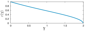
Figure 3: (Colour online) In the presence of nearest-neighbour dipolar interactions, the weathervane mode of KHAFM remains perfectly local, but the spin precession becomes elliptic with eccenticity $\varepsilon(D)$ given by Eq. (13) and plotted here.

V Spin-wave approach

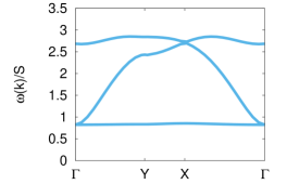
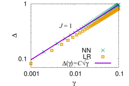
Figure 4: (Colour online) (a) Spin-wave spectrum of kagome antiferromagnet with nearest neighbour Heiseberg ($J=1$) and $\gamma=0.1J$ long-range dipolar interactions. The dipolar interactions gap the spectrum, but the lowest band remains nearly dispersionless. (b) The gap scales as $\sqrt{\gamma}$ both for long-range (LR) and truncated nearest-neighbour (NN) dipolar interactions.

The findings of the previous section can be confirmed in the spin-wave theory and extended to long-range dipolar interactions. The quantum fluctuations around the classical ground state are naturally obtained after the linearised Holstein–Primakoff transformation

$${S_{i}^{x}}(\mathbf{k}) = \sqrt{\frac{S}{2}}\left[c_{i}^{\dagger}(\mathbf{k})+c_{i}(-\mathbf{k})\right]$$ (14)

$${S_{i}^{y}}(\mathbf{k}) = i\sqrt{\frac{S}{2}}\left[c_{i}^{\dagger}(\mathbf{k})-c_{i}(-\mathbf{k})\right]$$

$${S_{i}^{z}}(\mathbf{k}) = \sqrt{N}S\delta_{\mathbf{k},0}\,e^{-i\mathbf{k}\cdot\mathbf{r}_{i}}-\frac{1}{\sqrt{N}}\sum_{\mathbf{k}^{\prime}}c_{i}^{\dagger}(\mathbf{k}^{\prime})c_{i}(\mathbf{k}^{\prime}-\mathbf{k}),$$

with boson operators $\left[c_{i}(\mathbf{k}),\;c_{j}^{\dagger}(\mathbf{k}^{\prime})\right]=\delta_{i,j}\delta_{\mathbf{k},\mathbf{k^{\prime}}}$. As before, the components of the spin vector are obtained in each spin’s local coordinate frame. Truncating the Hamiltonian beyond the quadratic terms and diagonalizing the resulting quadratic form by the means of a standard Bogolyubov transformation, we arrive at the Hamiltonian

$$H = H^{(0)}+\sum_{\mathbf{k}}\sum_{i}\omega_{i}(\mathbf{k})$$

$$+\sum_{\mathbf{k}}\sum_{i}\omega_{i}(\mathbf{k})\left[a_{i}^{\dagger}(\mathbf{k})a_{i}(\mathbf{k})+a_{i}^{\dagger}(-\mathbf{k})a_{i}(-\mathbf{k})\right],$$

where $a_{i}(\mathbf{k})$ and $a^{\dagger}_{i}(\mathbf{k})$ are Bogolyubov-transformed boson operators and the real eigenvalues $\omega_{i}(\mathbf{k})$ indicate stable ground-state spin configuration.

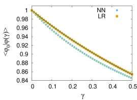
Figure 5: (Colour online) Overlap of the flat-band eigenstate $\phi_{0}$ at $\gamma=0$ with the eigenstate $\phi(\gamma)$ for $\gamma\neq 0$. For small $\gamma$ both nearest-neighbour (NN) and long-range (LR) dipolar interaction lead to the same functional form (16).

We have performed the diagonalizaton of the spin-wave Hamiltonian for nearest-neighbour dipolar interactions and for the energy of the flat-band to obtain expression (12). For the long-range dipolar interactions we diagonalize spin-wave Hamiltonian numerically.

The surprising finding is that including the long-range terms has barely any effect on the flat band. Fig. 4 shows the full spin-wave spectrum for the case of long-range dipolar interactions with $\gamma=0.1J$. While the size of the gap is a bit reduced by the inclusion of these terms, the scaling of the gap with $\gamma$ remains the same, $\Delta\propto\sqrt{\gamma}$ – see Fig. 4. While we understand this scaling analytically for the nearest-neighbour model – see Eq. (12) – its insensitivity to the long-range terms may appear puzzling.

In order to understand the reason, it is instructive to take another look at the microscopic picture of the weathervane mode developed in Section IV for the nearest-neighbour case. Two observations are in order. Firstly, the same logic that we used to argue that spin $\mathbf{S}_{0}$ in Fig. 2 was unaffected if two of its neighbours, $\mathbf{S}_{1}$ and $\mathbf{S}_{2}$, tilted away from their respective equilibrium positions by opposite angles also tells us that $\mathbf{S}_{0}$ remains unaffected by the weathervane mode even in the presence of longer-range terms. Each pair of equidistant spins (out of the six spins participating in the weathervane mode) generates no torque on $\mathbf{S}_{0}$ since the two spins tilt in opposite directions. As for the spins further away from the hexagon hosting this mode, we notice that the six oscillating spins still always add to zero. This implies that the spin dipole moment associated with the weathervane mode is zero and hence the leading term in the multipole expansion describing the interaction of other spins with the weathervane mode is at best quadrupolar and hence rapidly decays with distance. Therefore it is natural to expect that the weathervane mode remains essentially local which, in turn, explains the observed flatness of the band. The main effect of the longer-range rerms will be to renormalise couplings in the EOMs such as Eq. (11) while preserving their structure.

We also consider the overlap of the eigenstates in the zero $\phi_{0}$ and finite-energy $\phi(\gamma)$ flat-bands as $\gamma$ increases. In Fig. 5 overlaps for nearest-neighbour dipolar interactions and long-range dipolar interactions are plotted. In both cases we observe a continuous decrease of the overlap with the increase of $\gamma$ with both curves fitting well to a functional form

$$\langle\phi_{0}|\phi(\gamma)\rangle=\frac{1}{\sqrt{1+a\gamma/\left(J+b\gamma/2\right)}},$$ (16)

where in the long-range case $a=0.75$ and $b=0$ are renormalisation factors of dipolar interactions in $x$ and $y$ components of the flat-band eigenstates. For the nearest-neighbour dipolar interactions both parameters $a$ and $b$ are equal to $1$ and equation above can also be obtained from the equations of motion Eq. (11).

VI Conjugate variables representation and Maxwellian counting

In this section, we make contact with the lore on excitations and frustrated magnets, in particular the ideas of constraint counting used to derive the size of the zero-energy space of excitations.

In the absence of dipolar interactions, the origin of the flat band at zero energy is understood by noting that, for $n$-component spins represented by unit length vectors, the number of degrees of freedom per unit cell of three spins is $D_{n}=3(n-1)$. At the same time, the constraints per unit cell imposed by the Hamiltonian are evaluated as $K_{n}=2n$, as two momentless triangles inhabit each unit cell, and momentlessness requires one constraint on each of the $n$ spin components.

For Heisenberg spins, these are balanced, $D_{3}=K_{3}$, while for for XY spins, $n=2$, there exist ground states satisfying one more constraint than they use degrees of freedom: $D_{2}-K_{2}=-1$. For the subset of coplanar ground states, an unconstrained degree of freedom therefore remains, as there are three out of plane degrees of freedom for the two remaining constraints on the total spin of the two triangles in the unit cell.

The spin wave spectrum for three spins consists of three bands, as pairs of conjugate variables, $p_{\eta}(k),q_{\eta}(k)$ for each of the three modes $\eta=1\ldots 3$ at wavevector $k$ appear in the canonical Hamiltonian:

$$H=\sum_{\eta,k}\alpha_{\eta}(k)p^{2}+\beta_{\eta}(k)q^{2}\ .$$ (17)

The spin-wave frequencies are thus computed similarly to harmonic oscillator modes

$$\omega_{\eta}(k)=\sqrt{\alpha_{\eta}(k)\beta_{\eta}(k)}\ .$$ (18)

The underconstraint identified above translates into the vanishing of one band of coefficients (out of six), say of all

$$\alpha_{1}(k)\equiv 0\ .$$ (19)

From this perspective, the possibility of lifting the mode to a flat finite frequency band looks outlandish – for a vanishing frequency, Eq. 19 imposes no constraints on the behaviour of $\beta_{1}(k)$ in order to satisfy $\omega_{1}(k)=\sqrt{\alpha_{1}(k)\beta_{1}(k)}\equiv 0$. However, for $\omega_{1}(k)=\sqrt{\alpha_{1}(k)\beta_{1}(k)}\equiv\Omega>0$, one requires the momentum dependence of $\beta_{1}(k)=\Omega^{2}/\alpha_{1}(k)$ to be the inverse of that of $\alpha_{1}(k)$.

The way this is resolved is that both $\alpha_{1}(k)$ and $\beta_{1}(k)$ are constant functions of $k$, related to the hexagonal motifs of the weathervane modes: they correspond to the two (in- and out-of-plane) components of the spin wave. The spin wave mode corresponds to an excitation of these components with the the relative phase shifted by $\pi/2$. This describes elliptical precession of spins with an eccentricity discussed above.

This ‘doubled’ flat band structure of the kagome Heisenberg excitations has, to our knowledge, not yet been identified even for the much-studied pure nearest-neighbour Heisenberg model. It is a remarkable fact that it remains stable to the addition of the dipolar interactions and manifests itself in the band flatness at a finite frequency $\Omega>0$.

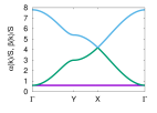
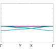
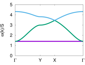
Figure 6: (Colour online) Spectra of conjugate variables coefficients $\alpha$ (left) and $\beta$ (right) for nearest-neighbour dipolar interactions ${\gamma=0.2J}$. Full spin-wave spectrum constructed from $\alpha$ and $\beta$ as ${\omega=\sqrt{\alpha\beta}}$.

VII Extensions to other systems

VII.1 Dzyaloshinskii–Moriya interactions

Having established the existence of weathervane modes and corresponding flat magnon bands for KHAFM with dipolar interactions, a natural question is whether this phenomenon is confined to this specific model. In this section we show that a number of extensions and modifications of our model preserve the flatness of the magnon band. The first, most straightforward generalisation of our model involves additional Dzyaloshinskii–Moriya (DM) interactions $\delta H_{\text{DM}}=\sum_{\langle i,j\rangle}\mathbf{D}_{ij}\cdot\left(\mathbf{S}_{i}\times\mathbf{S}_{j}\right)$, which should generically be present in kagomé systems Dzyaloshinskii (1957); Dzyaloshinsky (1958); Moriya (1960); Yildirim et al. (1994, 1995); Elhajal et al. (2002); Ballou et al. (2003); Cépas et al. (2008); Chernyshev and Zhitomirsky (2015) due to the lack of the inversion symmetry with respect to the mid-points of its bonds. These interactions are known to exist in materials with 2D kagomé planes such as the herbertsmithite Zorko et al. (2008) and jarosite Matan et al. (2006); Yildirim and Harris (2006) compounds. For a strictly 2D kagomé system (or if the kagomé plane is also a mirror plane), vectors $\mathbf{D}_{ij}$ must be strictly perpendicular to the plane. Moreover, if the inversion symmetry with respect to the sites of the lattice is not broken, the DM coupling parameter must be uniform, $\mathbf{D}_{ij}=-D\hat{\mathbf{x}}$, provided that all pairs $\langle i,j\rangle$ are ordered in an anticlockwise manner around lattice triangles.  Therefore, as long as $D>0$ (using the aforementioned sign convention), the DM interactions are not frustrating: by themselves, they stabilise a $120^{\circ}$ state with positive spin vorticity, and the two ground states of Hamiltonian (2) are already of this kind. This could be seen explicitly using the alternative expression for the Hamiltonian consisting of both Heisenberg and nearest-neighbour dipole–dipole interactions derived in Appendix A. With the addition of the DM interactions, the combined Hamiltonian becomes

$$H_{\text{KH+NND+DM}}=\sum_{\vartriangle}\left\{\frac{J+\gamma}{2}\,\mathbf{S}_{\vartriangle}^{2}\right.\\ -\gamma\mathbf{S_{\vartriangle}}\cdot\sum_{i\in\vartriangle}\hat{\mathbf{e}}_{i}\left(\mathbf{S}_{i}\cdot\hat{\mathbf{e}}_{i}\right)+\gamma\left[\sum_{i\in\vartriangle}\mathbf{S}_{i}\cdot\hat{\mathbf{e}}_{i}\right]^{2}\\ \left.-\left(D+\frac{\sqrt{3}}{2}\gamma\right)\sum_{\langle i\hookrightarrow j\rangle\in\vartriangle}\left(\mathbf{S}_{i}\times\mathbf{S}_{j}\right)\!\cdot\hat{\mathbf{x}}\right\}.$$ (20)

The inclusion of the DM term simply makes the coefficient in front of the last term bigger, and the magnitude of that term was already saturated by the ground state shown in Fig. 2. Moreover, this equation shows that as long as the antiferromagnetic Heisenberg coupling $J$ is strong enough to stabilise $120^{\circ}$ ground states, the spin configuration of Fig. 2 remains the ground state even for moderately negative DM coupling $-\sqrt{3}\gamma/2\leq D<0$ which, without the dipolar term, would stabilise the $120^{\circ}$ state of the opposite spin vorticity. (The only frustrating term in Eq. (20) is the second one, and it remains zero in all $120^{\circ}$ configurations).

A straightforward modification of the linearised EOMs (11) for the same weathervane mode now reads

$$\frac{\hbar}{S}\frac{dS^{x}_{2}}{dt} = 3\left(J+\frac{\gamma}{2}+\sqrt{3}D\right)S^{y}_{2},$$

$$\frac{\hbar}{S}\frac{dS^{y}_{2}}{dt} = -\left(3\gamma+2\sqrt{3}D\right)S^{x}_{2}.$$ (21)

The resulting frequency is

$${\hbar}\omega=3S\sqrt{\left(\gamma+\frac{2\sqrt{3}}{3}D\right)\left(J+\frac{\gamma}{2}+\sqrt{3}D\right)},$$ (22)

which, in the absence of dipolar interactions $\gamma=0$, reduces to the frequency of the flat mode found in Ref. [Chernyshev and Zhitomirsky, 2015]. Note, however, that while the addition of DM interactions (with all $\mathbf{D}_{ij}$ parallel to one another) reduces the symmetry of the Heisenberg Hamiltonian from SU(2) to U(1), the Goldstone theorem still guarantees the existence of a gapless mode, and a linearly-dispersive (at small $k$) mode was indeed found in in Ref. [Chernyshev and Zhitomirsky, 2015]. The weathervane mode, while flat, is not the lowest energy excitation in this case. This situation is changed dramatically in the presence of dipolar interactions, which further reduce the symmetry to $\mathbb{Z}_{2}$ thus completely gapping the spin waves. While for small $\gamma\ll D$ formerly gapless dispersive mode remains below that of the flat band for sufficiently strong dipolar term the flat-band can become again the lowest band in the spectrum (See Figure 7).

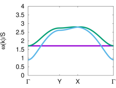
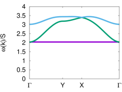
Figure 7: (Colour online) Full spin-wave spectrum for $J=1$, $D=0.2$ and $\gamma=0.01$ (top), $\gamma=0.1$ (bottom).

Note that irrespective of a particular choice of parameters, the flat band is always touched by another band, in full agreement with the counting argument of Ref. [Bergman et al., 2008].

VII.2 Dipolar-like interactions with arbitrary sign

Further generalisations of the model include considering the dipolar-type term with the negative coupling constant $\gamma<0$. We remind the reader that the coupling constant of the genuine dipole–dipole interaction is fixed: $\gamma_{\text{dp}}=g^{2}\mu_{\text{B}}^{2}/a^{3}$. However, a term of this type need not arise from dipole–dipole interactions. As was shown by Moriya Moriya (1960) and further elaborated by Yildirim et al. Yildirim et al. (1994, 1995), the superexchange mechanism in the presence of spin-orbit interactions leads to the spin–spin interaction of the general form

$$H_{ij}=J_{ij}\mathbf{S}_{i}\cdot\mathbf{S}_{j}+\mathbf{D}_{ij}\cdot\left(\mathbf{S}_{i}\times\mathbf{S}_{j}\right)+\sum_{\alpha,\beta}{S}_{i}^{\alpha}\Gamma_{ij}^{\alpha\beta}{S}_{j}^{\beta}$$ (23)

where the first two terms describe the familiar Heisenberg and Dzyaloshinskii–Moriya interactions while the last term is the anisotropic exchange term characterised by a symmetric traceless tensor $\Gamma^{\alpha\beta}$. Note that the dipolar coupling in Eq. (3) is exactly of this type, but whenever this term is generated by superexchange rather than actual dipole–dipole interactions, the sign of $\gamma$ can be arbitrary. Moreover, if we insist on the full set of symmetries of a kagomé plane, we can argue that such dipolar-like interaction is just one of the two couplings consistent with these symmetries. Specifically, note that a real symmetric traceless tensor $\Gamma^{\alpha\beta}$ has five independent components. For the purpose of this argument let us choose an orthogonal set of axes for a particular bond as follows: let the $z$- axis align with the bond, the $y$-axis lie in the kagomeé plane and the $x$-axis be perpendicular to it (in accordance with the choice of the $x$-axis direction made earlier). The symmetries of the kagomé plane include $(y,z)$ and $(x,y)$ mirror planes, with the former coinciding with the kagomeé plane itself and the latter being perpendicular to the bond at its midpoint. As a result, the Hamiltonian should be invariant under $x\to-x$ and $z\to-z$ transformations (with the components of spins transforming accordingly). Therefore $\Gamma^{xy}=\Gamma^{xz}=\Gamma^{yz}=0$, leaving us with just two independent parameters. Choosing $\gamma$, the dipolar-like coupling, to be one of them, the other parameter is $3\delta=\Gamma^{yy}-\Gamma^{xx}$, the difference between in-plane and out-of-plane couplings for spin components orthogonal to the bond.

Therefore, the most general bilinear spin-spin interaction consistent with the symmetries of the kagomé lattice can be written as

$$H_{ij}=(J+\gamma+\delta)\mathbf{S}_{i}\cdot\mathbf{S}_{j}+\mathbf{D}_{ij}\cdot\left(\mathbf{S}_{i}\times\mathbf{S}_{j}\right)\\ -3\gamma\left(\mathbf{S}_{i}\cdot\hat{\mathbf{r}}_{ij}\right)\left(\mathbf{S}_{j}\cdot\hat{\mathbf{r}}_{ij}\right)-3\delta S_{i}^{x}S_{j}^{x},$$ (24)

where $\mathbf{D}_{ij}$ is a vector in the $\mathbf{\hat{x}}$ (i.e., out-of-plane) direction with the aforementioned sign convention. Given the superexchange origin of these terms, the signs of coupling constants $\gamma$ and $\delta$ can now be arbitrary, and we should only concern ourselves with the nearest-neighbour interactions since this mechanism is exponentially suppressed with distance.

Let us first consider the case of $\gamma<0$ and $\delta=0$. While it may not immediately obvious what the ground sate(s) of Hamiltonian (4) or, equivalently (38) with $\gamma<0$ might be – after all, the individual terms in Eq. (38) are now minimised by different spin configurations – it turns out that the energy in minimised by the all-in/all-out $120^{\circ}$ states where all $\mathbf{S}_{i}\parallel\hat{\mathbf{e}}_{i}$. In other words, the two ground states are obtained from the ground states in the positive $\gamma$ case by rotating all spins by $\pi/2$. In fact, the Hamiltonian with the negative “dipolar” coupling $\gamma<0$ is less frustrated than the identical Hamiltonian with $\gamma>0$ due to the dominant nature of the third term in Eq. (38); the ground state energy for $\gamma<0$ is $1.5\lvert\gamma\rvert$ lower than that for $\gamma>0$ of the same magnitude. As a result, even a weak ferromagnetic Heisenberg coupling $J<0$ does not immediately destabilise this state: As long as $\lvert J\rvert<\lvert\gamma\rvert/2$, the ground state remains the all-in/all-out $120^{\circ}$ state. For strong ferromagnetic coupling $\lvert J\rvert>\lvert\gamma\rvert/2$ the energy is minimised when all three spins are parallel to one another and perpendicular to the kagomé plane.

An additional DM term with $D>0$ can only further stabilise the all-in/all-out $120^{\circ}$ state as it would counteract the frustrating effect of the last term in Eq. (38), which by itself would favour the state with the opposite spin vorticity.

Without the DM term, the linearised EOMs for the weathervane mode become

$$\frac{\hbar}{S}\frac{dS^{x}_{2}}{dt}=3\left(J+\frac{3\lvert\gamma\rvert}{2}\right)S^{y}_{2},\quad\frac{\hbar}{S}\frac{dS^{y}_{2}}{dt}=-9\lvert\gamma\rvert S^{x}_{2},$$ (25)

and the frequency of such a mode is now given by

$${\hbar}\omega=9S\sqrt{\lvert\gamma\rvert\left(\frac{J}{3}+\frac{\lvert\gamma\rvert}{2}\right)}.$$ (26)

For small $\lvert\gamma\rvert\ll J$ it is still proportional to the square root of the coupling constant $\lvert\gamma\rvert$, but it is higher than that given by Eq (12) for $\gamma>0$ of the same magnitude. This is not surprising, since we already saw that the system is less frustrated for $\gamma<0$ and has deeper energy minima.

Modifications of Eqs. (25) and (26) for the case of additional DM interactions are straightforward since the contributions of the DM terms into the effective magnetic field acting on a given spin are invariant under the rotations of all spins by the same angle in the plane of the lattice and hence they contribute to the EOMs in exactly the same way they do for the $\gamma>0$ case (see Eqs. (VII.1,22)):

$$\frac{\hbar}{S}\frac{dS^{x}_{2}}{dt} = 3\left(J+\frac{3\lvert\gamma\rvert}{2}+\sqrt{3}D\right)S^{y}_{2},$$

$$\frac{\hbar}{S}\frac{dS^{y}_{2}}{dt} = -\left(9\lvert\gamma\rvert+2\sqrt{3}D\right)S^{x}_{2}.$$ (27)

The frequency of such mode becomes

$${\hbar}\omega=3S\sqrt{\left(3\lvert\gamma\rvert+\frac{2\sqrt{3}}{3}D\right)\left(J+\frac{3\lvert\gamma\rvert}{2}+\sqrt{3}D\right)}.$$ (28)

VII.3 XXZ anisotropy

Finally, we turn our attention to the case of $\delta\neq 0$ (see Eq. (24)). Working out the full phase diagram of this model is beyond the scope of our paper. While strong out-of-plane coupling can easily cant the spins, it has been found that in the absence of dipolar-like terms ($\gamma=0$), the ground states of (24) for reasonably small positive values of $\delta\in(0,J/2)$ and arbitrarily small DM interactions with $D>0$ are $120^{\circ}$ states with positive spin vorticity Essafi et al. (2016). Moreover, such ground states are stabilised for any value of $\delta$ (positive or negative) by a sufficiently strong DM term. As we have argued, the presence of short-range dipolar-like terms ($\gamma\neq 0$) would then merely break the remaining global O(2) symmetry down to $\mathbb{Z}_{2}$. The upshot is that as long as the ground states of our system are either the ones described in Section III, or the all-in/all-out states described in this section, the above analysis applies.

Therefore, for $\gamma>0$, the linearised EOMs for the weathervane mode become

$$\frac{\hbar}{S}\frac{dS^{x}_{2}}{dt} = 3\left(J+\frac{\gamma}{2}+\delta+\sqrt{3}D\right)S^{y}_{2},$$

$$\frac{\hbar}{S}\frac{dS^{y}_{2}}{dt} = -\left(3\gamma+6\delta+2\sqrt{3}D\right)S^{x}_{2}.$$ (29)

The resulting frequency is

$${\hbar}\omega=3S\sqrt{\left(\gamma+2\delta+\frac{2\sqrt{3}}{3}D\right)\left(J+\frac{\gamma}{2}+\delta+\sqrt{3}D\right)}.$$ (30)

Meantime, for $\gamma<0$, Eqs. (VII.2) and (28) become generalised to

$$\frac{\hbar}{S}\frac{dS^{x}_{2}}{dt} = 3\left(J+\frac{3\lvert\gamma\rvert}{2}+\delta+\sqrt{3}D\right)S^{y}_{2},$$

$$\frac{\hbar}{S}\frac{dS^{y}_{2}}{dt} = -\left(9\lvert\gamma\rvert+6\delta+2\sqrt{3}D\right)S^{x}_{2}.$$ (31)

The frequency of the weathervane mode becomes

$${\hbar}\omega=3S\sqrt{\left(3\lvert\gamma\rvert+2\delta+\frac{2\sqrt{3}}{3}D\right)\left(J+\frac{3\lvert\gamma\rvert}{2}+\delta+\sqrt{3}D\right)}.$$ (32)

We conclude that the flat magnon band is a very generic feature of the classical kagomé antiferromagnets. It is very robust and its nature is largely independent of the details of the interactions, as long as their net effect is to stabilise one of the $120^{\circ}$ planar ground states with positive spin vorticity.

VII.4 The fate of the Goldstone mode

It is interesting to note that in the absence of dipolar-like terms in the Hamiltonian given by Eq. (24), either Dzyaloshinskii–Moriya ($D\neq 0$) or XXZ anisotropy ($\delta\neq 0$) are sufficient to lift the flat band to a finite energyChernyshev and Zhitomirsky (2015), as can be clearly seen from Eqs. (30) and (32). Nevertheless, both of these terms keep the full spin wave spectrum gapless: they only break the SU(2) symmetry of the Heisenberg Hamiltonian down to U(1), and the Goldstone theorem still guarantees the existence of a gapless mode with $\omega_{q\to 0}\to 0$. A dipolar-like term in Eq. (24) is the only term that breaks the symmetry of the Hamiltonian down to $\mathbb{Z}_{2}$ and thus opens the gap in the spin wave spectrum. A straightforward analysis of uniform deviations of all spins from their equilibrium positions for the case of $\gamma>0$ yields the following equations of motion:

$$\frac{\hbar}{S}\frac{dS^{x}}{dt} = 12\gamma S^{y},$$

$$\frac{\hbar}{S}\frac{dS^{y}}{dt} = -\left(6J+9\gamma+6\delta+2\sqrt{3}D\right)S^{x}.$$ (33)

The frequency of this mode becomes

$${\hbar}\omega=6S\sqrt{\gamma\left(2J+3\gamma+2\delta+\frac{2\sqrt{3}}{3}D\right)}.$$ (34)

A similar calculation for $\gamma<0$ yields

$$\frac{\hbar}{S}\frac{dS^{x}}{dt} = 12\left|\gamma\right|S^{y},$$

$$\frac{\hbar}{S}\frac{dS^{y}}{dt} = -\left(6J+3\left|\gamma\right|+6\delta+2\sqrt{3}D\right)S^{x},$$ (35)

and consequently

$${\hbar}\omega=6S\sqrt{\left|\gamma\right|\left(2J+\left|\gamma\right|+2\delta+\frac{2\sqrt{3}}{3}D\right)}.$$ (36)

Therefore, for small dipolar interactions the gap in the spin wave spectrum is always proportional to $\sqrt{\left|\gamma\right|}$, but it need not correspond to the flat band, which may be shifted to higher energy by DM interactions or XXZ anisotropy.

Curiously, in the absence of DM interactions or XXZ anisotropy, the uniform mode softens at $J=-|\gamma|/2$ on the ferromagnetic side ($J<0$), i.e. precisely at the point where the nature of the ground state changes from the $120^{\circ}$ arrangement of spins ($|J|<|\gamma|/2$) to the fully-polarised out-of-plane state ($|J|>|\gamma|/2$). This may appear puzzling since the transition between the two ground states as a function of $J/K$ is a typical first-order, level-crossing transition not requiring any mode softening. However, it is easy to check that exactly at $J=\gamma/2<0$ the energy of a uniformly canted $120^{\circ}$ arrangement of spins becomes independent on the canting angle (which is consistent with the notion of a transition from the uncanted to the maximally-canted, i.e. ferromagnetic state). It is this degeneracy of the ground state with respect the canting angle that is reflected in the vanishing frequency of the uniform mode.

VIII Discussion and outlook

In summary, we have discovered a remarkable stability of the dispersionlessness of the band of weathervane modes of the classical kagome Heisenberg antiferromagnet. In particular, we have identified the dipolar interactions as a particularly impressive case in point, given that it removes the continuous Heisenberg symmetry with its concomitant gaplessness of the mode spectrum, moving the flat band upwards along with the rest of the spectrum, while generating only a weak dispersion despite its long-range nature. The latter feature we were able to connect to a Heisenberg version of the self-screening effect found in the frustrated pyrochlore Ising system known as dipolar spin iceCastelnovo et al. (2012).

More broadly, the mechanism we have identified for the persistence of the dispersionlessness applies in a broad range of settings, including the (previously observed) cases of XXZ and DM anisotropies, the latter of which we have discussed in a more general setting here. In the two former cases, a combination of experimental information of the size of the gap, and the location of the flat band (at energies above the gap) may be used to glean information about the relative size of perturbations to the ideal Heisenberg hamiltonian.

Overall, we have found that the flat band of weathervane modes is remarkably robust in classical kagome magnets. There are a number of further settings in which one can study their properties, and particular scope for their manipulation. One natural item here is the role of an applied magnetic field, given its application connects to the well-known situation that at saturation, flat band physics enters perhaps in its most natural way as the hopping problem of flipped spin excitations on top of the ‘ferromagnetic’ background, leading to features such as a discontinuous jump in the magnetisation Schulenburg et al. (2002); Zhitomirsky and Tsunetsugu (2005); Schmidt et al. (2006); Derzhko et al. (2007).

While a number of distinct setups yield dispersionless bands, the consideration of lattices such as the kagome case discussed here in detail exhibiting strong geometrical frustration has long been a natural route to induce such physics.

In this respect rare-earth geometrically frustrated magnets are among the most obvious candidates to address the flat-band effects in the spin-waves excitation spectra. The existence of the dispersionless modes at finite energy sharply manifest itself in inelastic neutron scattering as a finite energy, almost ${\mathbf{k}}$-independent resonance Maestro and Gingras (2004); Quilliam et al. (2007); Lee et al. (2000). A recent experimental study of the stalwart frustrated gadolinium gallium garnet $\rm Gd_{3}Ga_{5}O_{12}$ was aimed to precisely address experimental manifestation of a dispersionless band in inelastic neutron scattering d’Ambrumenil et al. (2015). In this compound, magnetic ions are arranged in a 3D hyperkagomé structure and flat-band emerges as a lowest spin-wave band above the saturated ferromagnetic ground state in the strong magnetic field. As this field varies it effectively plays a role of a chemical potential controlling the population of excitations in a band. Importantly, there the presence of dipolar interaction does not preserve the dispersionlessness to the same degree as in the 2D kagome case, on account of the interplay of the noncoplanarity of the triangles on the hyperkagome lattice and the ’spin–orbit’ coupling of the dipolar interaction.

Regarding potential experimental realisation of the 2D physics, recent studies have identified a rare-earth kagomé compound $\text{Mg}_{2}\text{Gd}_{3}\text{Sb}_{3}\text{O}_{14}$ Dun et al. (2016). The $120^{\circ}$ ground state is found to be stabilised by weak dipolar interactions and according to our studies the spin-wave spectrum of the model Hamiltonian used for $\text{Mg}_{2}\text{Gd}_{3}\text{Sb}_{3}\text{O}_{14}$ in Ref. [Dun et al., 2016] should contain a gapped flat-band mode, subject of course to possible interference of other, yet to be identified, weak terms in the Hamiltonian. Hence the presence of the flat band could be identified already at zero magnetic field in the inelastic neutron scattering experiments and in a variety of low-temperature behaviour of thermodynamic quantities.

On top of this, there exists a rising number of systems which realise kagomé lattice structure and where dipolar interactions play important or dominant role, such as dipolar nano-arrays Wang et al. (2006); Möller and Moessner (2006), thin films of frustrated materials Leusink et al. (2014); Bhuiyan et al. (2005); LeBlanc et al. (2013); Tomeno et al. (1999) or dipoles in optical lattices Pupillo et al. (2009); Yao et al. (2012); Bettles et al. (2015). Our analysis demonstrates effects of self-screening of dipolar interactions in such system and interesting mechanism of lifting the formerly zero-energy flat band by squeezing the corresponding localised modes. The investigation of strong many-body effects in such (nearly) flat bands and their manifestation in accessible experimental probes is an interesting direction for future research.

More broadly, dispersionless bands in the quasiparticle spectrum provide a unique setup in which kinetic energy of corresponding modes is entirely quenched and all the dynamics is due to disorder, interaction or quantum statistics effects. Recent interest in flat-bands has addressed many-body instabilities, thermodynamic effects, exotic topological phases and novel states that could be realised there Parameswaran et al. (2013); Bergholtz and Liu (2013); Derzhko et al. (2015). Our study suggests flat bands may be more stable than one might have feared.

IX Acknowledgements

We would like thank Benoit Douçot, Chris Henley and Oleg Petrenko for enlightening discussions and V. Ravi Chandra for collaboration on a related project. The authors would like to acknowledge the DFG SFB 1143 grant, which provided partial support for the collaborative effort at MPIPKS, Dresden. MM was supported in part by the ERC UQUAM grant; KS was supported in part by the NSF DMR-1411359 grant.

Appendix A Dipolar Hamiltonian on one lattice triangle

In this appendix we derive an alternative expression for the Hamiltonian consisting of both Heisenberg and nearest-neighbour dipole–dipole interactions on one lattice triangle. For concreteness, let us focus on the shaded triangle hosting spins $\mathbf{S}_{0}$, $\mathbf{S}_{1}$ and $\mathbf{S}_{2}$ in Fig. 2. We begin by introducing unit vectors $\hat{\mathbf{e}}_{i}$ pointing from the centre of a given triangle to each of its corners. It is easy to see that $\hat{\mathbf{r}}_{ij}=\left(\hat{\mathbf{e}}_{j}-\hat{\mathbf{e}}_{i}\right)/\sqrt{3}$. Straightforward but somewhat tedious algebra then yields

$$\frac{1}{2}\sum_{i,j\in\vartriangle}\left(\mathbf{S}_{i}\cdot\hat{\mathbf{r}}_{ij}\right)\left(\mathbf{S}_{j}\cdot\hat{\mathbf{r}}_{ij}\right)\\ =-\frac{1}{3}\left[\sum_{i\in\vartriangle}\mathbf{S}_{i}\cdot\hat{\mathbf{e}}_{i}\right]^{2}+\frac{1}{3}\mathbf{S_{\vartriangle}}\cdot\sum_{i\in\vartriangle}\hat{\mathbf{e}}_{i}\left(\mathbf{S}_{i}\cdot\hat{\mathbf{e}}_{i}\right)\\ +\frac{1}{6}\sum_{i,j\in\vartriangle}\left(\mathbf{S}_{i}\times\mathbf{S}_{j}\right)\!\cdot\!\left(\hat{\mathbf{e}}_{i}\times\hat{\mathbf{e}}_{j}\right)\\ =-\frac{1}{3}\left[\sum_{i\in\vartriangle}\mathbf{S}_{i}\cdot\hat{\mathbf{e}}_{i}\right]^{2}+\frac{1}{3}\mathbf{S_{\vartriangle}}\cdot\sum_{i\in\vartriangle}\hat{\mathbf{e}}_{i}\left(\mathbf{S}_{i}\cdot\hat{\mathbf{e}}_{i}\right)\\ +\frac{1}{2\sqrt{3}}\sum_{\langle i\hookrightarrow j\rangle\in\vartriangle}\left(\mathbf{S}_{i}\times\mathbf{S}_{j}\right)\!\cdot\hat{\mathbf{x}},$$ (37)

where notation $\langle i\hookrightarrow j\rangle$ in the last sum indicates anticlockwise ordering of spins around the triangle in each pair; $\hat{\mathbf{x}}$ is the unit vector directed out of plane, consistent with the our choice of local coordinate frames throughout this paper. The coefficient of $1/2$ on the left-hand side of this equation is to prevent double counting of pairs of spins.

Therefore the Hamiltonian (4) for one lattice triangle can be written, up to a constant, as

$$H_{\vartriangle}=\frac{J+\gamma}{2}\,\mathbf{S}_{\vartriangle}^{2}-\gamma\mathbf{S_{\vartriangle}}\cdot\sum_{i\in\vartriangle}\hat{\mathbf{e}}_{i}\left(\mathbf{S}_{i}\cdot\hat{\mathbf{e}}_{i}\right)\\ +\gamma\left[\sum_{i\in\vartriangle}\mathbf{S}_{i}\cdot\hat{\mathbf{e}}_{i}\right]^{2}-\frac{\gamma\sqrt{3}}{2}\sum_{\langle i\hookrightarrow j\rangle\in\vartriangle}\left(\mathbf{S}_{i}\times\mathbf{S}_{j}\right)\!\cdot\hat{\mathbf{x}}.$$ (38)

The reason for writing the Hamiltonian in such a form is that it allows for an easy incorporation of additional Dzyaloshiskii–Moriya terms, since the last term of Eq. (38) is of exactly that form. The one term whose role is not transparent is the second one. However, as long as we are dealing with the states with $\mathbf{S}_{\vartriangle}=0$ (and we know this to be true e.g., for the ground state(s) of this Hamiltonian for $J,\gamma\geq 0$), the second term vanishes. The rest of the terms are not frustrated in the sense that the ground state minimises each of them individually for $J,\gamma\geq 0$. This statement may not be obvious in reference to the last term, so it might be useful to rewrite it using

$$\frac{\sqrt{3}}{2}\sum_{\langle i\hookrightarrow j\rangle\in\vartriangle}\left(\mathbf{S}_{i}\times\mathbf{S}_{j}\right)\!\cdot\hat{\mathbf{x}}=\frac{9}{4}\,S^{2}\,\mathbf{v}_{\vartriangle}\cdot\hat{\mathbf{x}},$$ (39)

where $\mathbf{v}_{\vartriangle}={2}/{(3\sqrt{3}S^{2})}\,\sum_{\langle i\hookrightarrow j\rangle\in\vartriangle}\mathbf{S}_{i}\times\mathbf{S}_{j}$ is the vector vorticity of a three-spin configuration normalised so that $\lvert\mathbf{v}\rvert_{\text{max}}=1$. The vorticity is maximised by the coplanar $120^{\circ}$ arrangements of spins, and $v_{\vartriangle}^{x}=1$ for the ground states considered here.

References

- Ramirez et al. (1999) A. P. Ramirez, A. Hayashi, R. J. Cava, R. Siddharthan, and B. S. Shastry, Nature 399, 333 (1999).
- Castelnovo et al. (2012) C. Castelnovo, R. Moessner, and S. L. Sondhi, Annu. Rev. Condens. Matter Phys. 3, 35 (2012), arXiv:1112.3793 .
- Moessner and Chalker (1998a) R. Moessner and J. T. Chalker, Phys. Rev. Lett. 80, 2929 (1998a), cond-mat/9712063 .
- Moessner and Chalker (1998b) R. Moessner and J. T. Chalker, Phys. Rev. B 58, 12049 (1998b), arXiv:cond-mat/9807384 .
- Chalker et al. (1992) J. T. Chalker, P. C. W. Holdsworth, and E. F. Shender, Phys. Rev. Lett. 68, 855 (1992).
- Ritchey et al. (1993) I. Ritchey, P. Chandra, and P. Coleman, Phys. Rev. B 47, 15342 (1993).
- Shender et al. (1993) E. F. Shender, V. B. Cherepanov, P. C. W. Holdsworth, and A. J. Berlinsky, Phys. Rev. Lett. 70, 3812 (1993).
- Harris et al. (1992) A. B. Harris, C. Kallin, and A. J. Berlinsky, Phys. Rev. B 45, 2899 (1992).
- Chernyshev and Zhitomirsky (2015) A. L. Chernyshev and M. E. Zhitomirsky, Phys. Rev. B 92, 144415 (2015), arXiv:1508.06632 .
- Parameswaran et al. (2013) S. A. Parameswaran, R. Roy, and S. L. Sondhi, C. R. Phys. 14, 816 (2013), arXiv:1302.6606 .
- Bergholtz and Liu (2013) E. J. Bergholtz and Z. Liu, Int. J. Mod. Phys. B 27, 1330017 (2013), arXiv:1308.0343 .
- Derzhko et al. (2015) O. Derzhko, J. Richter, and M. Maksymenko, Int. J. Mod. Phys. B 29, 1530007 (2015), arXiv:1502.02729 .
- Vidal et al. (1998) J. Vidal, R. Mosseri, and B. Douçot, Phys. Rev. Lett. 81, 5888 (1998), cond-mat/9806068 .
- Dóra et al. (2011) B. Dóra, J. Kailasvuori, and R. Moessner, Phys. Rev. B 84, 195422 (2011), arXiv:1104.0416 .
- Du et al. (2017) L. Du, X. Zhou, and G. A. Fiete, Phys. Rev. B 95, 035136 (2017), arXiv:1608.07488 .
- Schulenburg et al. (2002) J. Schulenburg, A. Honecker, J. Schnack, J. Richter, and H.-J. Schmidt, Phys. Rev. Lett. 88, 167207 (2002), cond-mat/0108498 .
- Zhitomirsky and Tsunetsugu (2005) M. E. Zhitomirsky and H. Tsunetsugu, Prog. Theor. Phys. Suppl. 160, 361 (2005), cond-mat/0506327 .
- Schmidt et al. (2006) H.-J. Schmidt, J. Richter, and R. Moessner, J. Phys. A: Math. Gen. 39, 10673 (2006), arXiv:cond-mat/060464 .
- Derzhko et al. (2007) O. Derzhko, J. Richter, A. Honecker, and H.-J. Schmidt, Low Temp. Phys. 33, 745 (2007), (Fiz. Nizk. Temp. 33, 982–996), cond-mat/0612281 .
- den Hertog and Gingras (2000) B. C. den Hertog and M. J. P. Gingras, Phys. Rev. Lett. 84, 3430 (2000).
- Isakov et al. (2005) S. V. Isakov, R. Moessner, and S. L. Sondhi, Phys. Rev. Lett. 95, 217201 (2005).
- Castelnovo et al. (2008) C. Castelnovo, R. Moessner, and S. L. Sondhi, Nature 451, 42 (2008), arXiv:0710.5515 .
- d’Ambrumenil et al. (2015) N. d’Ambrumenil, O. A. Petrenko, H. Mutka, and P. P. Deen, Phys. Rev. Lett. 114, 227203 (2015), arXiv:1501.03493 .
- Huse and Rutenberg (1992) D. A. Huse and A. D. Rutenberg, Phys. Rev. B 45, 7536 (1992).
- Chubukov (1992) A. Chubukov, Phys. Rev. Lett. 69, 832 (1992).
- von Delft and Henley (1992) J. von Delft and C. L. Henley, Phys. Rev. Lett. 69, 3236 (1992), cond-mat/9208011 .
- Chern and Moessner (2013) G.-W. Chern and R. Moessner, Phys. Rev. Lett. 110, 077201 (2013), arXiv:1207.4752 .
- Maksymenko et al. (2015) M. Maksymenko, V. R. Chandra, and R. Moessner, Phys. Rev. B 91, 184407 (2015), arXiv:1502.05960 .
- Dzyaloshinskii (1957) I. E. Dzyaloshinskii, Zh. Eksp. Teor. Fiz. 32, 1547 (1957), [Sov. Phys. JETP 5, 1259–1262 (1957)].
- Dzyaloshinsky (1958) I. Dzyaloshinsky, J. Phys. Chem. Solids 4, 241 (1958).
- Moriya (1960) T. Moriya, Phys. Rev. 120, 91 (1960).
- Yildirim et al. (1994) T. Yildirim, A. B. Harris, O. Entin-Wohlman, and A. Aharony, Phys. Rev. Lett. 73, 2919 (1994).
- Yildirim et al. (1995) T. Yildirim, A. B. Harris, A. Aharony, and O. Entin-Wohlman, Phys. Rev. B 52, 10239 (1995).
- Elhajal et al. (2002) M. Elhajal, B. Canals, and C. Lacroix, Phys. Rev. B 66, 014422 (2002), cond-mat/0202194 .
- Ballou et al. (2003) R. Ballou, B. Canals, M. Elhajal, C. Lacroix, and A. S. Wills, J. Magn. Magn. Mater. 262, 465 (2003).
- Cépas et al. (2008) O. Cépas, C. M. Fong, P. W. Leung, and C. Lhuillier, Phys. Rev. B 78, 140405 (2008), arXiv:0806.0393 .
- Zorko et al. (2008) A. Zorko, S. Nellutla, J. van Tol, L. C. Brunel, F. Bert, F. Duc, J.-C. Trombe, M. A. de Vries, A. Harrison, and P. Mendels, Phys. Rev. Lett. 101, 026405 (2008), arXiv:0804.3107 .
- Matan et al. (2006) K. Matan, D. Grohol, D. G. Nocera, T. Yildirim, A. B. Harris, S. H. Lee, S. E. Nagler, and Y. S. Lee, Phys. Rev. Lett. 96, 247201 (2006).
- Yildirim and Harris (2006) T. Yildirim and A. B. Harris, Phys. Rev. B 73, 214446 (2006).
- Note (1) Here we adopt the site ordering convention of Refs. [\rev@citealpnumElhajal2002] and [\rev@citealpnumBallou2003]; other authors prefer ordering them along the 1D chains of spins, which results in alternating directions of between up- and down-triangles – see e.g. Refs. [\rev@citealpnumCepas2008], [\rev@citealpnumChernyshev2015].
- Bergman et al. (2008) D. L. Bergman, C. Wu, and L. Balents, Phys. Rev. B 78, 125104 (2008), arXiv:0803.3628 .
- Note (2) The choice of the -axis for the out-of-plane direction is a consequence of aligning local -axes along each spin in their equilibrium state – a standard choice for the Holstein–Primakoff transformations in the spin-wave theory. This makes referring to the XXZ anisotropy later in text somewhat awkward, but we prefer it to changing the axis labelling convention halfway through the manuscript.
- Essafi et al. (2016) K. Essafi, O. Benton, and L. D. C. Jaubert, Nat. Commun. 7, 10297 (2016), arXiv:1508.00113 .
- Maestro and Gingras (2004) A. G. D. Maestro and M. J. P. Gingras, J. Phys.: Condens. Matter 16, 3339 (2004).
- Quilliam et al. (2007) J. A. Quilliam, K. A. Ross, A. G. Del Maestro, M. J. P. Gingras, L. R. Corruccini, and J. B. Kycia, Phys. Rev. Lett. 99, 097201 (2007).
- Lee et al. (2000) S.-H. Lee, C. Broholm, T. H. Kim, W. Ratcliff, and S. W. Cheong, Phys. Rev. Lett. 84, 3718 (2000).
- Dun et al. (2016) Z. L. Dun, J. Trinh, K. Li, M. Lee, K. W. Chen, R. Baumbach, Y. F. Hu, Y. X. Wang, E. S. Choi, B. S. Shastry, A. P. Ramirez, and H. D. Zhou, Phys. Rev. Lett. 116, 157201 (2016), arXiv:1601.01575 .
- Wang et al. (2006) R. F. Wang, C. Nisoli, R. S. Freitas, J. Li, W. McConville, B. J. Cooley, M. S. Lund, N. Samarth, C. Leighton, V. H. Crespi, and P. Schiffer, Nature 439, 303 (2006).
- Möller and Moessner (2006) G. Möller and R. Moessner, Phys. Rev. Lett. 96, 237202 (2006).
- Leusink et al. (2014) D. Leusink, F. Coneri, M. Hoek, S. Turner, H. Idrissi, G. Van Tendeloo, and H. Hilgenkamp, APL Materials 2, 032101 (2014).
- Bhuiyan et al. (2005) M. S. Bhuiyan, M. Paranthaman, S. Sathyamurthy, A. Goyal, and K. Salama, Journal of Materials Research 20, 904 (2005).
- LeBlanc et al. (2013) M. D. LeBlanc, M. L. Plumer, J. P. Whitehead, and B. W. Southern, Phys. Rev. B 88, 094406 (2013).
- Tomeno et al. (1999) I. Tomeno, H. N. Fuke, H. Iwasaki, M. Sahashi, and Y. Tsunoda, J. Appl. Phys. 86, 3853 (1999).
- Pupillo et al. (2009) G. Pupillo, A. Micheli, H. P. Büchler, and P. Zoller, in Cold molecules: Creation and applications, edited by R. V. Krems, B. Friedrich, and W. C. Stwalley (Taylor & Francis, 2009) arXiv:0805.1896.
- Yao et al. (2012) N. Y. Yao, C. R. Laumann, A. V. Gorshkov, S. D. Bennett, E. Demler, P. Zoller, and M. D. Lukin, Phys. Rev. Lett. 109, 266804 (2012), arXiv:1207.4479 .
- Bettles et al. (2015) R. J. Bettles, S. A. Gardiner, and C. S. Adams, Phys. Rev. A 92, 063822 (2015), arXiv:1410.4776 .