Nash Region of the Linear Deterministic Interference Channel with Noisy Output Feedback

Abstract

In this paper, the $\eta$-Nash equilibrium ($\eta$-NE) region of the two-user linear deterministic interference channel (IC) with noisy channel-output feedback is characterized for all $\eta>0$. The $\eta$-NE region, a subset of the capacity region, contains the set of all achievable information rate pairs that are stable in the sense of an $\eta$-NE. More specifically, given an $\eta$-NE coding scheme, there does not exist an alternative coding scheme for either transmitter-receiver pair that increases the individual rate by more than $\eta$ bits per channel use. Existing results such as the $\eta$-NE region of the linear deterministic IC without feedback and with perfect output feedback are obtained as particular cases of the result presented in this paper.

I System Model

Consider the two-user decentralized linear deterministic interference channel with noisy channel-output feedback (D-LD-IC-NOF) depicted in Figure 1. For all $i\in\{1,2\}$, with $j\in\{1,2\}\setminus\{i\}$, the number of bit-pipes between transmitter $i$ and its intended receiver is denoted by $\overrightarrow{n}_{ii}$; the number of bit-pipes between transmitter $i$ and its non-intended receiver is denoted by $n_{ji}$; and the number of bit-pipes between receiver $i$ and its corresponding transmitter is denoted by $\overleftarrow{n}_{ii}$. These six non-negative integer parameters describe the D-LD-IC-NOF in Figure 1.

At transmitter $i$, the channel-input $\boldsymbol{X}_{i,n}$ at channel use $n$, with $n\in\{1,2,\ldots,N_{i}\}$, is a $q$-dimensional binary vector ${\boldsymbol{X}_{i,n}=\left(X_{i,n}^{(1)},X_{i,n}^{(2)},\ldots,X_{i,n}^{(q)}\right)^{\textsf{T}}}\in\mathcal{X}_{i}$, with $\mathcal{X}_{i}=\{0,1\}^{q}$,

$$q=\displaystyle\max\left(\overrightarrow{n}_{11},\overrightarrow{n}_{22},n_{12},n_{21}\right),$$ (1)

and $N_{i}\in\mathds{N}$ is the block-length of transmitter-receiver pair $i$. At receiver $i$, the channel-output $\overrightarrow{\boldsymbol{Y}}_{i,n}$ at channel use $n$, with $n\in\{1,2,\ldots,\max\left(N_{1},N_{2}\right)\}$, is also a $q$-dimensional binary vector ${\overrightarrow{\boldsymbol{Y}}_{i,n}=\left(\overrightarrow{Y}_{i,n}^{(1)},\overrightarrow{Y}_{i,n}^{(2)},\ldots,\overrightarrow{Y}_{i,n}^{(q)}\right)^{\textsf{T}}}$. Let $\boldsymbol{S}$ be a $q\times q$ binary lower shift matrix. The input-output relation during channel use $n$ is given by

$$\overrightarrow{\boldsymbol{Y}}_{i,n} = \boldsymbol{S}^{q-\overrightarrow{n}_{ii}}\boldsymbol{X}_{i,n}+\boldsymbol{S}^{q-n_{ij}}\boldsymbol{X}_{j,n},$$ (2)

where ${\boldsymbol{X}_{i,n}=\left(0,0,\ldots,0\right)^{\textsf{T}}}$ for all $n>N_{i}$. The feedback signal $\boldsymbol{\overleftarrow{Y}}_{i,n}$ available at transmitter $i$ at the end of channel use $n$ is

$$\boldsymbol{\overleftarrow{Y}}_{i,n} = \boldsymbol{S}^{\left(\max(\overrightarrow{n}_{ii},n_{ij})-\overleftarrow{n}_{ii}\right)^{+}}\,\boldsymbol{\overrightarrow{Y}}_{i,n-d},\quad$$ (3)

where $d$ is a finite delay, additions and multiplications are defined over the binary field, and $(\cdot)^{+}$ is the positive part operator.

Without any loss of generality, the feedback delay is assumed to be equal to one channel use. Let $\mathcal{W}_{i}$ be the set of message indices of transmitter $i$. Transmitter $i$ sends the message index $W_{i}\in\mathcal{W}_{i}$ by transmitting the codeword ${\boldsymbol{X}_{i}=\left(\boldsymbol{X}_{i,1},\boldsymbol{X}_{i,2},\ldots,\boldsymbol{X}_{i,N_{i}}\right)\in\mathcal{X}_{i}^{N_{i}}}$, which is a binary $q\times N_{i}$ matrix. The encoder of transmitter $i$ can be modeled as a set of deterministic mappings $f_{i,1}^{(N)},f_{i,2}^{(N)},\ldots,f_{i,N_{i}}^{(N)}$, with $f_{i,1}^{(N)}:\mathcal{W}_{i}\times\mathds{N}\rightarrow\{0,1\}^{q}$ and for all $n\in\{2,3,\ldots,N_{i}\}$, $f_{i,n}^{(N)}:\mathcal{W}_{i}\times\mathds{N}\times\{0,1\}^{q\times(n-1)}\rightarrow\{0,1\}^{q}$, such that

$$\boldsymbol{X}_{i,1} = f_{i,1}^{(N)}\big{(}W_{i},\Omega_{i}\big{)}\mbox{ and }$$ (4a)

$$\boldsymbol{X}_{i,n} = f_{i,n}^{(N)}\big{(}W_{i},\Omega_{i},\boldsymbol{\overleftarrow{Y}}_{i,1},\boldsymbol{\overleftarrow{Y}}_{i,2},\ldots,\boldsymbol{\overleftarrow{Y}}_{i,n-1}\big{)},$$ (4b)

where $\Omega_{i}$ is a randomly generated index known by both transmitter $i$ and receiver $i$, while unknown by transmitter $j$ and receiver $j$.

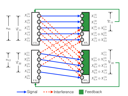
Figure 1: Two-user linear deterministic interference channel with noisy channel-output feedback at channel use $n$.

The decoder of receiver $i$ is defined by a deterministic function $\psi_{i}^{(N)}:\{0,1\}^{q\times N}\times\mathds{N}\rightarrow\mathcal{W}_{i}$. At the end of the communication, receiver $i$ uses the $q\times N$ binary matrix $\left(\overrightarrow{\boldsymbol{Y}}_{i,1},\overrightarrow{\boldsymbol{Y}}_{i,2},\ldots,\overrightarrow{\boldsymbol{Y}}_{i,N}\right)$ and $\Omega_{i}$ to obtain an estimate $\widehat{W}_{i}\in\mathcal{W}_{i}$ of the message index $W_{i}$, i.e., $\widehat{W}_{i}=\psi_{i}^{(N)}\left(\overrightarrow{\boldsymbol{Y}}_{i,1},\overrightarrow{\boldsymbol{Y}}_{i,2},\ldots,\overrightarrow{\boldsymbol{Y}}_{i,N},\Omega_{i}\right)$. Let $W_{i}$ be written as $c_{i,1}\,c_{i,2}\,\ldots\,c_{i,M_{i}}$ in binary form, with $M_{i}=\lceil\log_{2}|\mathcal{W}_{i}|\rceil$. Let also $\widehat{W}_{i}$ be written as $\widehat{c}_{i,1}\,\widehat{c}_{i,2}\,\ldots\,\widehat{c}_{i,M_{i}}$ in binary form.

A transmit-receive configuration for transmitter-receiver pair $i$, denoted by $s_{i}$, can be described in terms of the block-length $N_{i}$, the number of bits per block $M_{i}$, the channel-input alphabet $\mathcal{X}_{i}$, the codebook, the encoding functions $f_{i,1}^{(N)},f_{i,2}^{(N)},\ldots,f_{i,N_{i}}^{(N)}$, the decoding function $\psi_{i}^{(N)}$, etc.

The average bit error probability at decoder $i$ given the configurations $s_{1}$ and $s_{2}$, denoted by $p_{i}(s_{1},s_{2})$, is given by

$$p_{i}(s_{1},s_{2}) = \frac{1}{M_{i}}\displaystyle\sum_{\ell=1}^{M_{i}}\mathds{1}_{\left\{\widehat{c}_{i,\ell}\neq{c}_{i,\ell}\right\}}.$$ (5)

Within this context, a rate pair $(R_{1},R_{2})\in\mathds{R}_{+}^{2}$ is said to be achievable if it complies with the following definition.

Definition 1 (Achievable Rate Pairs)

A rate pair $(R_{1},R_{2})\in\mathds{R}_{+}^{2}$ is achievable if there exists at least one pair of configurations $(s_{1},s_{2})$ such that the decoding bit error probabilities $p_{1}(s_{1},s_{2})$ and $p_{2}(s_{1},s_{2})$ can be made arbitrarily small by letting the block-lengths $N_{1}$ and $N_{2}$ grow to infinity.

The aim of transmitter $i$ is to autonomously choose its transmit-receive configuration $s_{i}$, in order to maximize its achievable rate $R_{i}$. Note that the rate achieved by transmitter-receiver $i$ depends on both configurations $s_{1}$ and $s_{2}$ due to mutual interference. This reveals the competitive interaction between both links in the decentralized interference channel. The following section models this interaction using tools from game theory.

II The Two-User Interference Channel as a Game

The competitive interaction between the two transmitter-receiver pairs in the decentralized interference channel can be modeled by the following game in normal-form:

$$\mathcal{G}=\left(\mathcal{K},\left\{\mathcal{A}_{k}\right\}_{k\in\mathcal{K}},\left\{u_{k}\right\}_{k\in\mathcal{K}}\right).$$ (6)

The set $\mathcal{K}=\{1,2\}$ is the set of players, that is, the set of transmitter-receiver pairs. The sets $\mathcal{A}_{1}$ and $\mathcal{A}_{2}$ are the sets of actions of players $1$ and $2$, respectively. An action of a player $i\in\mathcal{K}$, which is denoted by $s_{i}\in\mathcal{A}_{i}$, is basically its transmit-receive configuration as described in Section I. The utility function of player $i$ is $u_{i}:\mathcal{A}_{1}\times\mathcal{A}_{2}\rightarrow\mathds{R}_{+}$ and it is defined as the information rate of transmitter $i$,

$$u_{i}(s_{1},s_{2})=\left\{\begin{array}[]{lcl}R_{i}=\frac{M_{i}}{N_{i}},&\mbox{if}&p_{i}(s_{1},s_{2})<\epsilon\\ 0,&&\mbox{otherwise,}\end{array}\right.$$ (7)

where $\epsilon>0$ is an arbitrarily small number.

This game formulation was first proposed in [1] and [2]. A class of transmit-receive configurations $\boldsymbol{s}^{*}=(s_{1}^{*},s_{2}^{*})\in\mathcal{A}_{1}\times\mathcal{A}_{2}$ that are particularly important in the analysis of this game is referred to as the set of $\eta$-Nash equilibria ($\eta$-NE), with $\eta>0$. This type of configuration satisfies the following definition.

Definition 2 ($\eta$-Nash equilibrium)

In the game ${\mathcal{G}=\left(\mathcal{K},\left\{\mathcal{A}_{k}\right\}_{k\in\mathcal{K}},\left\{u_{k}\right\}_{k\in\mathcal{K}}\right)}$, an action profile $(s_{1}^{*},s_{2}^{*})$ is an $\eta$-Nash equilibrium if for all $i\in\mathcal{K}$ and for all $s_{i}\in\mathcal{A}_{i}$, there exits an $\eta>0$ such that

$$u_{i}(s_{i},s_{j}^{*})\leqslant u_{i}(s_{i}^{*},s_{j}^{*})+\eta.$$ (8)

Let $(s_{1}^{*},s_{2}^{*})$ be an $\eta$-Nash equilibrium action profile of the game in (6). Then, none of the transmitters can increase its own information transmission rate more than $\eta$ bits per channel use by changing its own transmit-receive configuration and keeping the average bit error probability arbitrarily close to zero. Note that for $\eta$ sufficiently large, from Definition 2, any pair of configurations can be an $\eta$-NE. Alternatively, for $\eta=0$, the classical definition of Nash equilibrium is obtained [3]. In this case, if a pair of configurations is a Nash equilibrium ($\eta=0$), then each individual configuration is optimal with respect to each other. Hence, the interest is to describe the set of all possible $\eta$-NE rate pairs $(R_{1},R_{2})$ of the game in (6) with the smallest $\eta$ for which there exists at least one equilibrium configuration pair. The set of rate pairs that can be achieved at an $\eta$-NE is known as the $\eta$-Nash equilibrium region.

Definition 3 ($\eta$-NE Region)

Let $\eta>0$ be fixed. An achievable rate pair $(R_{1},R_{2})$ is said to be in the $\eta$-NE region of the game $\mathcal{G}=\left(\mathcal{K},\left\{\mathcal{A}_{k}\right\}_{k\in\mathcal{K}},\left\{u_{k}\right\}_{k\in\mathcal{K}}\right)$ if there exists a pair $(s_{1}^{*},s_{2}^{*})\in\mathcal{A}_{1}\times\mathcal{A}_{2}$ that is an $\eta$-NE and the following holds:

$$u_{1}(s_{1}^{*},s_{2}^{*})=R_{1} u_{2}(s_{1}^{*},s_{2}^{*})=R_{2}.$$ and (9)

The following section characterizes the $\eta$-NE region (Def. 3) of the two-user D-LD-IC-NOF in (6), denoted by $\mathcal{N}_{\eta}\left(\overrightarrow{n}_{11},\overrightarrow{n}_{22},n_{12},n_{21},\overleftarrow{n}_{11},\overleftarrow{n}_{22}\right)$, for fixed parameters $\big{(}\overrightarrow{n}_{11}$, $\overrightarrow{n}_{22}$, $n_{12}$, $n_{21}$, $\overleftarrow{n}_{11}$,$\overleftarrow{n}_{22}\big{)}\in\mathds{N}^{6}$ and for all $\eta>0$.

III Main Results

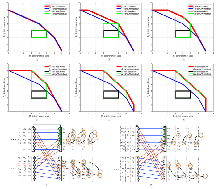
Figure 2: Capacity region $\mathcal{C}(7,6,4,4,0,0)$ (thin blue line) and $\eta$-NE region $\mathcal{N}_{\eta}(7,6,4,4,0,0)$ (thick black line) with $\eta$ chosen arbitrarily small. Fig. 2a shows the capacity region $\mathcal{C}(7,6,4,4,\overleftarrow{n}_{11},\overleftarrow{n}_{22})$ (thick red line) and the $\eta$-NE region $\mathcal{N}_{\eta}(7,6,4,4,\overleftarrow{n}_{11},\overleftarrow{n}_{22})$ (thin green line), with $\overleftarrow{n}_{11}\in\{0,1,2,3,4\}$ and $\overleftarrow{n}_{22}\in\{0,1,2,3,4\}$. Fig. 2b shows the capacity region $\mathcal{C}(7,6,4,4,5,\overleftarrow{n}_{22})$ (thick red line) and the $\eta$-NE region $\mathcal{N}_{\eta}(7,6,4,4,5,\overleftarrow{n}_{22})$ (thin green line), with $\overleftarrow{n}_{22}\in\{0,1,2,3,4\}$. Fig. 2c shows the capacity region $\mathcal{C}(7,6,4,4,6,\overleftarrow{n}_{22})$ (thick red line) and the $\eta$-NE region $\mathcal{N}_{\eta}(7,6,4,4,6,\overleftarrow{n}_{22})$ (thin green line), with $\overleftarrow{n}_{22}\in\{0,1,2,3,4\}$. Fig. 2d shows the capacity region $\mathcal{C}(7,6,4,4,7,\overleftarrow{n}_{22})$ (thick red line) and the $\eta$-NE region $\mathcal{N}_{\eta}(7,6,4,4,7,\overleftarrow{n}_{22})$ (thin green line), with $\overleftarrow{n}_{22}\in\{0,1,2,3,4\}$. Fig. 2e shows the capacity region $\mathcal{C}(7,6,4,4,7,5)$ (thick red line) and the $\eta$-NE region $\mathcal{N}_{\eta}(7,6,4,4,7,5)$ (thin green line). Fig. 2f shows the capacity region $\mathcal{C}(7,6,4,4,7,6)$ (thick red line) and the $\eta$-NE region $\mathcal{N}_{\eta}(7,6,4,4,7,6)$ (thin green line). Fig. 2g and Fig. 2h illustrate the achievability scheme for the equilibrium rate pair $(3,4)$ and $(5,4)$ in $\mathcal{N}_{\eta}{(7,6,4,4,5,0)}$.

The $\eta$-NE region is characterized in terms of two regions: the capacity region, denoted by $\mathcal{C}{\left(\overrightarrow{n}_{11},\overrightarrow{n}_{22},n_{12},n_{21},\overleftarrow{n}_{11},\overleftarrow{n}_{22}\right)}$ and a convex region, denoted by $\mathcal{B}_{\eta}{\left(\overrightarrow{n}_{11},\overrightarrow{n}_{22},n_{12},n_{21},\overleftarrow{n}_{11},\overleftarrow{n}_{22}\right)}$. In the following, the tuple $(\overrightarrow{n}_{11}$, $\overrightarrow{n}_{22}$, $n_{12}$, $n_{21}$, $\overleftarrow{n}_{11}$, $\overleftarrow{n}_{22})$ is used only when needed.

The capacity region $\mathcal{C}$ of the two-user LD-IC-NOF is described in Theorem $1$ in [4], which is a generalization of previous works in [5] and [6]. For all $\eta>0$, the convex region $\mathcal{B}_{\eta}$ is defined as follows:

$$\mathcal{B}_{\eta} = \Big{\{}(R_{1},R_{2}):\!L_{i}\!\leqslant\!R_{i}\!\leqslant\!U_{i},\!\mbox{ for all }i\in\{1,2\}\Big{\}},$$ (10)

where,

$$L_{i} =\left(\left(\overrightarrow{n}_{ii}-n_{ij}\right)^{+}-\eta\right)^{+}\mbox{ and }$$ (11a)

$$U_{i} =\max\left(\overrightarrow{n}_{ii},n_{ij}\right)-\Bigg{(}\min\left(\left(\overrightarrow{n}_{jj}\!-\!n_{ji}\right)^{+},n_{ij}\right)$$

$$\!-\! \!\bigg{(}\!\min\!\left(\!\left(\!\overrightarrow{n}_{jj}\!-\!n_{ij}\!\right)^{+}\!,\!n_{ji}\!\right)\!-\!\left(\!\max\!\left(\!\overrightarrow{n}_{jj},\!n_{ji}\!\right)\!-\!\overleftarrow{n}_{jj}\!\right)^{+}\!\bigg{)}^{+}\!\Bigg{)}^{+}\!+\!\eta,$$

with $i\in\{1,2\}$ and $j\in\{1,2\}\setminus\{i\}$. Theorem 1 uses the region $\mathcal{B}_{\eta}$ in (10) and the capacity region $\mathcal{C}$ to describe the $\eta$-NE region $\mathcal{N}_{\eta}$.

Theorem 1

Let $\eta>0$ be fixed. The $\eta$-NE region $\mathcal{N}_{\eta}$ of the two-user D-LD-IC-NOF with parameters $\overrightarrow{n}_{11}$, $\overrightarrow{n}_{22}$, $n_{12}$, $n_{21}$, $\overleftarrow{n}_{11}$ and $\overleftarrow{n}_{22}$, is $\mathcal{N}_{\eta}=\mathcal{C}\cap\mathcal{B}_{\eta}$.

Figure 2 shows the capacity region $\mathcal{C}$ and the $\eta$-NE region $\mathcal{N}_{\eta}$ of a channel with parameters $\overrightarrow{n}_{11}=7$, $\overrightarrow{n}_{22}=6$, $n_{12}=4$, $n_{21}=4$ and different values for $\overleftarrow{n}_{11}$ and $\overleftarrow{n}_{22}$, with $\eta$ chosen arbitrarily small. Note that when $\overleftarrow{n}_{11}\in\{0,1,2,3,4\}$ and $\overleftarrow{n}_{22}\in\{0,1,2,3,4\}$ (Figure 2a), it follows that $\mathcal{N}_{\eta}{(7,6,4,4,\overleftarrow{n}_{11},\overleftarrow{n}_{22})}=\mathcal{N}_{\eta}{(7,6,4,4,0,0)}$. Thus, in this case the use of feedback in any of the transmitter-receiver pairs does not enlarge the $\eta$-Nash region. Alternatively, when $\overleftarrow{n}_{11}>4$ and $\overleftarrow{n}_{22}\in\{0,1,2,3,4\}$ (Figures 2b, 2c and 2d), the resulting $\eta$-Nash region is strictly larger than in the previous case. A similar effect is observed in Figures 2e and 2f. This observation implies the existence of a threshold on each feedback parameter $\overleftarrow{n}_{11}$ and $\overleftarrow{n}_{22}$ beyond which the $\eta$-Nash region is enlarged. The exact values of $\overleftarrow{n}_{11}$ and $\overleftarrow{n}_{22}$, given a fixed tuple $(\overrightarrow{n}_{11}$, $\overrightarrow{n}_{22}$, $n_{12}$, $n_{21})$, beyond which the $\eta$-Nash region can be enlarged is presented in [7]. Figure 2g and Figure 2h show the coding schemes to achieve the rate pairs $(3,4)$ and $(5,4)$, respectively, when $\overleftarrow{n}_{11}=5$ and $\overleftarrow{n}_{22}=0$. In Figure 2g, note that common randomness is used by transmitter-receiver pair $2$ to prevent transmitter-receiver pair $1$ from increasing its individual rate. More specifically, the bits $\tilde{b}_{1}$, $\tilde{b}_{2}$, $\tilde{b}_{3}$, …are known by both transmitter $2$ and receiver $2$. The use of common randomness is also observed in [8, 9] and [10]. Common randomness reflects a competitive behavior between both transmitter-receiver pairs. In Figure 2g, common randomness is not used by transmitter-receiver pair $2$ and thus, transmitter-receiver pair $1$ achieves a higher rate at an $\eta$-NE with respect to the previous example. This suggests a more altruistic behavior.

The $\eta$-NE region $\mathcal{N}_{\eta}$ without feedback, i.e., when $\overleftarrow{n}_{11}=0$ and $\overleftarrow{n}_{22}=0$ (Theorem $1$ in [8]), is $\mathcal{N}_{\eta}{(\overrightarrow{n}_{11},\overrightarrow{n}_{22},n_{12},n_{21},0,0)}$. The $\eta$-NE region with perfect feedback i.e., $\overleftarrow{n}_{11}=\max(\overrightarrow{n}_{11},n_{12})$ and $\overleftarrow{n}_{22}=\max(\overrightarrow{n}_{22},n_{21})$ (Theorem $1$ in [9]), is $\mathcal{N}_{\eta}(\overrightarrow{n}_{11}$, $\overrightarrow{n}_{22}$, $n_{12}$, $n_{21}$, $\max(\overrightarrow{n}_{11},n_{12})$, $\max(\overrightarrow{n}_{22},n_{21}))$. From the comments above, it is interesting to highlight the following inclusions:

$$\mathcal{N}_{\eta} \Big{(}\overrightarrow{n}_{11},\overrightarrow{n}_{22},n_{12},n_{21},0,0\Big{)}\subseteq$$ (12)

$$\mathcal{N}_{\eta} \Big{(}\overrightarrow{n}_{11},\overrightarrow{n}_{22},n_{12},n_{21},\overleftarrow{n}_{11},\overleftarrow{n}_{22}\Big{)}\subseteq$$

$$\mathcal{N}_{\eta} \Big{(}\overrightarrow{n}_{11},\overrightarrow{n}_{22},n_{12},n_{21},\max\left(\overrightarrow{n}_{11},n_{12}\right),\max\left(\overrightarrow{n}_{22},n_{21}\right)\Big{)},$$

for all $\eta>0$. The inclusions above might appear trivial, however, enlarging the set of actions often leads to paradoxes (Braess Paradox [11]) in which the new game possesses equilibria at which players obtain smaller individual benefits and/or smaller total benefit. Nonetheless, letting both transmitter-receiver pairs to use feedback does not induce this type of paradoxes with respect to the case without feedback.

IV Proofs

To prove Theorem 1, the first step is to show that a rate pair $(R_{1},R_{2})$, with $R_{i}<L_{i}$ or $R_{i}>U_{i}$ for at least one $i\in\{1,2\}$, is not achievable at an $\eta$-equilibrium for all $\eta>0$. That is,

$$\mathcal{N}_{\eta}\subseteq\mathcal{C}\cap\mathcal{B}_{\eta}.$$ (13)

The second step is to show that, for all $\eta>0$, any point in $\mathcal{C}\cap\mathcal{B}_{\eta}$ can be achievable at an $\eta$-equilibrium. That is,

$$\mathcal{N}_{\eta}\supseteq\mathcal{C}\cap\mathcal{B}_{\eta},$$ (14)

which proves the equality $\mathcal{N}_{\eta}=\mathcal{C}\cap\mathcal{B}_{\eta}$.

Proof of (13)

The proof of (13) is completed by the following lemmas.

Lemma 1

A rate pair $(R_{1},R_{2})\in\mathcal{C}$, with either $R_{1}<L_{1}$ or $R_{2}<L_{2}$ is not achievable at an $\eta$-equilibrium for all $\eta>0$.

Proof:

The proof of Lemma 1 is presented in [7]. ∎

The intuition behind this proof is that the rate ${R_{i}=\left(\overrightarrow{n}_{ii}-n_{ij}\right)^{+}}$ is always achievable independently of the coding scheme of transmitter-receiver pair $j$. To achieve ${R_{i}=\left(\overrightarrow{n}_{ii}-n_{ij}\right)^{+}}$ transmitter $i$ uses the most significant bit-pipes, which are interference free, to transmit new bits at each channel use $n$.

Lemma 2

A rate pair $(R_{1},R_{2})\in\mathcal{C}$, with either $R_{1}>U_{1}$ or $R_{2}>U_{2}$ is not achievable at an $\eta$-equilibrium for all $\eta>0$.

Proof:

The proof of Lemma 2 is presented in [7]. ∎

This proof is based on the fact that at an $\eta$-NE, transmitter $j$ might re-transmit some of the bits previously transmitted by transmitter $i$. The interference produced by those re-transmitted bits at receiver $i$ can be eliminated if they were received interference free during previous channel uses. This allows transmitter $i$ to use the bit-pipes interfered with by those re-transmitted bits to send new information bits at each channel use. The key point of this proof is to show that the maximum number of bits that can be re-transmitted at an $\eta$-NE is upper bounded.

Proof of (14)

Consider a modification of the coding scheme with noisy feedback presented in [4], which combines rate splitting [12], block Markov superposition coding [13] and backward decoding [14]. The novelty with respect to [4] consists of allowing users to introduce common randomness as suggested in [8] and [9].

Consider without any loss of generality that $N=N_{1}=N_{2}$. Let $W_{i}^{(t)}\in\{1,2,\ldots,2^{NR_{i}}\}$ and $\Omega_{i}^{(t)}\in\{1,2,\ldots,2^{NR_{i,R}}\}$ denote the message index and the random message index sent by transmitter $i$ during the $t$-th block, with $t\in\{1,2,\ldots,T\}$, respectively. Following a rate-splitting argument, assume that $\left(W_{i}^{(t)},\Omega_{i}^{(t)}\right)$ is represented by the indices $\left(W_{i,C1}^{(t)},\Omega_{i,R1}^{(t)},W_{i,C2}^{(t)},\Omega_{i,R2}^{(t)},W_{i,P}^{(t)}\right)\in\{1,2,\ldots,2^{NR_{i,C1}}\}\times\{1,2,\ldots,2^{NR_{i,R1}}\}\times\{1,2,\ldots,2^{NR_{i,C2}}\}\times\{1,2,\ldots,2^{NR_{i,R2}}\}\times\{1,2,\ldots,2^{NR_{i,P}}\}$, where $R_{i}=R_{i,C1}+R_{i,C2}+R_{i,P}$ and $R_{i,R}=R_{i,R1}+R_{i,R2}$. The rate $R_{i,R}$ is the number of transmitted bits that are known by both transmitter $i$ and receiver $i$ per channel use, and thus it does not have an impact on the information rate $R_{i}$.

The codeword generation follows a four-level superposition coding scheme. The indices $W_{i,C1}^{(t-1)}$ and $\Omega_{i,R1}^{(t-1)}$ are assumed to be decoded at transmitter $j$ via the feedback link of transmitter-receiver pair $j$ at the end of the transmission of block $t-1$. Therefore, at the beginning of block $t$, each transmitter possesses the knowledge of the indices $W_{1,C1}^{(t-1)}$, $\Omega_{1,R1}^{(t-1)}$, $W_{2,C1}^{(t-1)}$ and $\Omega_{2,R1}^{(t-1)}$. In the case of the first block $t=1$, the indices $W_{1,C1}^{(0)}$, $\Omega_{1,R1}^{(0)}$, $W_{2,C1}^{(0)}$ and $\Omega_{1,R2}^{(0)}$ are assumed to be known by all transmitters and receivers. Using these indices both transmitters are able to identify the same codeword in the first code-layer. This first code-layer, which is common for both transmitter-receiver pairs, is a sub-codebook of $2^{N\left(R_{1,C1}+R_{2,C1}+R_{1,R1}+R_{2,R1}\right)}$ codewords. Denote by $\boldsymbol{u}\left(W_{1,C1}^{(t-1)},\Omega_{1,R1}^{(t-1)},W_{2,C1}^{(t-1)},\Omega_{2,R1}^{(t-1)}\right)$ the corresponding codeword in the first code-layer. The second codeword is chosen by transmitter $i$ using $\left(W_{i,C1}^{(t)},\Omega_{i,R1}^{(t)}\right)$ from the second code-layer, which is a sub-codebook of $2^{N\left(R_{i,C1}+R_{i,R1}\right)}$ codewords corresponding to the codeword $\boldsymbol{u}\left(W_{1,C1}^{(t-1)},\Omega_{1,R1}^{(t-1)},W_{2,C1}^{(t-1)},\Omega_{2,R1}^{(t-1)}\right)$. Denote by $\boldsymbol{u}_{i}\left(W_{1,C1}^{(t-1)},\Omega_{1,R1}^{(t-1)},W_{2,C1}^{(t-1)},\Omega_{2,R1}^{(t-1)},W_{i,C1}^{(t)},\Omega_{i,R1}^{(t)}\right)$ the corresponding codeword in the second code-layer. The third codeword is chosen by transmitter $i$ using $\left(W_{i,C2}^{(t)},\Omega_{i,R2}^{(t)}\right)$ from the third code-layer, which is a sub-codebook of $2^{N\left(R_{i,C2}+R_{i,R2}\right)}$ codewords corresponding to the codeword $\boldsymbol{u}_{i}\left(W_{1,C1}^{(t-1)},\Omega_{1,R1}^{(t-1)},W_{2,C1}^{(t-1)},\Omega_{2,R1}^{(t-1)},W_{i,C1}^{(t)},\Omega_{i,R1}^{(t)}\right)$. Denote by $\boldsymbol{v}_{i}\Big{(}W_{1,C1}^{(t-1)},\Omega_{1,R1}^{(t-1)}$, $W_{2,C1}^{(t-1)},\Omega_{2,R1}^{(t-1)}$, $W_{i,C1}^{(t)},\Omega_{i,R1}^{(t)}$, $W_{i,C2}^{(t)},\Omega_{i,R2}^{(t)}\Big{)}$ the corresponding codeword in the third code-layer. The fourth codeword is chosen by transmitter $i$ using $W_{i,P}^{(t)}$ from the fourth code-layer, which is a sub-codebook of $2^{N\,R_{i,P}}$ codewords corresponding to the codeword $\boldsymbol{v}_{i}\Big{(}W_{1,C1}^{(t-1)},\Omega_{1,R1}^{(t-1)}$, $W_{2,C1}^{(t-1)},\Omega_{2,R1}^{(t-1)}$, $W_{i,C1}^{(t)},\Omega_{i,R1}^{(t)}$, $W_{i,C2}^{(t)},\Omega_{i,R2}^{(t)}\Big{)}$. Denote by $\boldsymbol{x}_{i,P}\Big{(}W_{1,C1}^{(t-1)},\Omega_{1,R1}^{(t-1)}$, $W_{2,C1}^{(t-1)},\Omega_{2,R1}^{(t-1)}$, $W_{i,C1}^{(t)},\Omega_{i,R1}^{(t)}$, $W_{i,C2}^{(t)},\Omega_{i,R2}^{(t)},W_{i,P}^{(t)}\Big{)}$ the corresponding codeword in the fourth code-layer. Finally, the codeword $\boldsymbol{x}_{i}\Big{(}W_{1,C1}^{(t-1)},\Omega_{1,R1}^{(t-1)}$, $W_{2,C1}^{(t-1)},\Omega_{2,R1}^{(t-1)}$, $W_{i,C1}^{(t)},\Omega_{i,R1}^{(t)}$, $W_{i,C2}^{(t)},\Omega_{i,R2}^{(t)},W_{i,P}^{(t)}\Big{)}$ to be sent during block $t\in\{1,2,\ldots,T\}$ is a simple concatenation of the previous codewords, i.e., ${\boldsymbol{x}_{i}=\left(\boldsymbol{u}_{i}^{\textsf{T}},\boldsymbol{v}_{i}^{\textsf{T}},\boldsymbol{x}_{i,P}^{\textsf{T}}\right)^{\textsf{T}}}\in\{0,1\}^{q\times N}$, where the message indices have been dropped for ease of notation.

The decoder follows a backward decoding scheme. In the following, this coding scheme is referred to as a randomized Han-Kobayashi coding scheme with noisy feedback (R-HK-NOF) and it is described in [7]. The rest of the proof consists of showing that the R-HK-NOF coding scheme is capable of achieving an $\eta$-NE with $(R_{1},R_{2})\in\mathcal{C}\cap\mathcal{B}_{\eta}$ for all $\eta>0$, subject to a proper choice of the rates $R_{i,R1}$ and $R_{i,R2}$, for all $i\in\{1,2\}$.

Lemma 3

The achievable region of the randomized Han-Kobayashi coding scheme for the D-LD-IC-NOF is the set of non-negative rates $\Big{(}R_{1,C1}$, $R_{1,R1}$, $R_{1,C2}$, $R_{1,R2}$, $R_{1,P}$, $R_{2,C1}$, $R_{2,R1}$, $R_{2,C2}$, $R_{2,R2}$, $R_{2,P}\Big{)}$ that satisfy the following conditions for all $i\in\{1,2\}$ and $j\in\{1,2\}\setminus\{i\}$:

$$R_{j,C1}+R_{j,R1} \leqslant \theta_{1,i},$$ (15a)

$$R_{i}+R_{j,C}+R_{j,R} \leqslant \theta_{2,i},$$ (15b)

$$R_{j,C2}+R_{j,R2} \leqslant \theta_{3,i},$$ (15c)

$$R_{i,P} \leqslant \theta_{4,i},$$ (15d)

$$R_{i,P}+R_{j,C2}+R_{j,R2} \leqslant \theta_{5,i},$$ (15e)

$$R_{i,C2}+R_{i,P} \leqslant \theta_{6,i},\mbox{ and }$$ (15f)

$$R_{i,C2}+R_{i,P}+R_{j,C2}+R_{j,R2} \leqslant \theta_{7,i},$$ (15g)

where,

$$\theta_{1,i} = \left(n_{ij}-\left(\max\left(\overrightarrow{n}_{ii},n_{ij}\right)-\overleftarrow{n}_{ii}\right)^{+}\right)^{+},$$ (16a)

$$\theta_{2,i} = \max\left(\overrightarrow{n}_{ii},n_{ij}\right),$$ (16b)

$$\theta_{3,i} = \min\left(n_{ij},\left(\max\left(\overrightarrow{n}_{ii},n_{ij}\right)-\overleftarrow{n}_{ii}\right)^{+}\right),$$ (16c)

$$\theta_{4,i} = \left(\overrightarrow{n}_{ii}-n_{ji}\right)^{+},$$ (16d)

$$\theta_{5,i} = \max\Big{(}\left(\overrightarrow{n}_{ii}-n_{ji}\right)^{+},$$ (16e)

$$\min\left(n_{ij},\left(\max\left(\overrightarrow{n}_{ii},n_{ij}\right)-\overleftarrow{n}_{ii}\right)^{+}\right)\Big{)},$$

$$\theta_{6,i} = \min\left(n_{ji},\left(\max\left(\overrightarrow{n}_{jj},n_{ji}\right)-\overleftarrow{n}_{jj}\right)^{+}\right)$$ (16f)

$$-\min\big{(}\left(n_{ji}-\overrightarrow{n}_{ii}\right)^{+},\left(\max\left(\overrightarrow{n}_{jj},n_{ji}\right)-\overleftarrow{n}_{jj}\right)^{+}\big{)}$$

$$+\left(\overrightarrow{n}_{ii}-n_{ji}\right)^{+},\mbox{ and }$$

$$\theta_{7,i} = \max\big{(}\min\big{(}n_{ij},\left(\max\left(\overrightarrow{n}_{ii},n_{ij}\right)-\overleftarrow{n}_{ii}\right)^{+}\big{)},$$ (16g)

$$\min\big{(}n_{ji},\left(\max\left(\overrightarrow{n}_{jj},n_{ji}\right)-\overleftarrow{n}_{jj}\right)^{+}\big{)}$$

$$-\min\big{(}\left(n_{ji}-\overrightarrow{n}_{ii}\right)^{+},\left(\max\left(\overrightarrow{n}_{jj},n_{ji}\right)-\overleftarrow{n}_{jj}\right)^{+}\big{)}$$

$$+\left(\overrightarrow{n}_{ii}-n_{ji}\right)^{+}\big{)}.$$

Proof:

The proof of Lemma 3 is presented in [7]. ∎

The set of inequalities in (15) can be written in terms of the transmission rates $R_{1}=R_{1,C1}+R_{1,C2}+R_{1,P}$ and $R_{2}=R_{2,C1}+R_{2,C2}+R_{2,P}$ to observe that the R-HK-NOF achieves all the rates $(R_{1},R_{2})\in\mathcal{C}$, when $R_{1,R}=R_{2,R}=0$.

The following lemma shows than when both transmitter-receiver links use the R-HK-NOF scheme and one of them unilaterally changes its coding scheme, it obtains a rate improvement that can be upper bounded.

Lemma 4

Let $\eta>0$ be fixed and let the rate tuple $\boldsymbol{R}=(R_{1,C}-\frac{\eta}{6},R_{1,R}-\frac{\eta}{6},R_{1,P}-\frac{\eta}{6},R_{2,C}-\frac{\eta}{6},R_{2,R}-\frac{\eta}{6},R_{2,P}-\frac{\eta}{6})$ be achievable with the R-HK-NOF such that $R_{1}=R_{1,P}+R_{1,C}-\frac{1}{3}\eta$ and $R_{2}=R_{2,P}+R_{2,C}-\frac{1}{3}\eta$. Then, any unilateral deviation of transmitter-receiver pair $i$ by using any other coding scheme leads to a transmission rate $R_{i}^{\prime}$ that satisfies $R_{i}^{\prime}\leqslant\max\left(\overrightarrow{n}_{ii},n_{ij}\right)-(R_{j,C}+R_{j,R})+\frac{2}{3}\eta$.

Proof:

The proof of Lemma 4 is presented in [7]. ∎

Lemma 4 reveals the relevance of the random symbols $\Omega_{1}$ and $\Omega_{2}$ used by the R-HK-NOF. Even though the random symbols used by transmitter $j$ do not increase the effective transmission rate of transmitter-receiver pair $j$, they strongly limit the rate improvement transmitter-receiver pair $i$ can obtain by deviating from the R-HK-NOF coding scheme. This observation can be used to show that the R-HK-NOF can be an $\eta$-NE, when both $R_{1,R}$ and $R_{2,R}$ are properly chosen. The following lemma formalizes this intuition.

Lemma 5

Let $\eta>0$ be fixed and let the rate tuple $\boldsymbol{R}=(R_{1,C}-\frac{\eta}{6},R_{1,R}-\frac{\eta}{6},R_{1,P}-\frac{\eta}{6},R_{2,C}-\frac{\eta}{6},R_{2,R}-\frac{\eta}{6},R_{2,P}-\frac{\eta}{6})$ be achieved by using the R-HK-NOF, with

$$R_{i,C}+R_{i,P}+R_{j,C}+R_{j,R} = \max(\overrightarrow{n}_{ii},n_{ij})+\frac{2}{3}\eta,$$ (17)

for all $i\in\{1,2\}$. Then, the rate pair $(R_{1},R_{2})$, with $R_{i}=R_{i,C}+R_{i,P}-\frac{1}{3}\eta$ is achievable at an $\eta$-Nash equilibrium.

Proof:

The proof of Lemma 5 is presented in [7]. ∎

The following lemma shows that all the rate pairs $(R_{1},R_{2})\in\mathcal{C}\cap\mathcal{B}_{\eta}$ are achievable by the R-HK-NOF coding scheme at an $\eta$-NE, for all $\eta>0$.

Lemma 6

Let $\eta>0$ be fixed. Then, for all rate pairs $(R_{1},R_{2})\in\mathcal{C}\cap\mathcal{B}_{\eta}$, there always exists at least one $\eta$-NE transmit-receive configuration pair $(s_{1}^{*},s_{2}^{*})\in\mathcal{A}_{1}\times\mathcal{A}_{2}$, such that $u_{1}(s_{1}^{*},s_{2}^{*})=R_{1}$ and $u_{2}(s_{1}^{*},s_{2}^{*})=R_{2}$.

Proof:

The proof of Lemma 6 is presented in [7]. ∎

This proof consists of showing that the set of inequalities in (15) and (17) leads to a set of rate pairs identical to $\mathcal{C}\cap\mathcal{B}_{\eta}$. This concludes the proof of Theorem 1.

V Conclusions

In this paper, the $\eta$-NE region of the D-LD-IC-NOF has been characterized for all $\eta>0$. This region contains the $\eta$-NE region without feedback studied in [8] and is contained within the $\eta$-NE region with perfect channel-output feedback studied in [9].

References

- [1] R. D. Yates, D. Tse, and Z. Li, “Secret communication on interference channels,” in Proc. IEEE International Symposium on Information Theory (ISIT), Toronto, Canada, Jul. 2008.
- [2] R. Berry and D. N. C. Tse, “Information theoretic games on interference channels,” in Proc. IEEE International Symposium on Information Theory (ISIT), Toronto,Canada, Jul. 2008.
- [3] J. F. Nash, “Equilibrium points in -person games,” Proc. National Academy of Sciences of the United States of America, vol. 36, no. 1, pp. 48–49, Jan. 1950.
- [4] V. Quintero, S. M. Perlaza, I. Esnaola, and J.-M. Gorce, “Approximate capacity region of the two-user Gaussian interference channel with noisy channel-output feedback,” (Submitted to) IEEE Trans. Inf. Theory, Nov 2016. [Online]. Available: https://arxiv.org/pdf/1611.05322.pdf
- [5] G. Bresler and D. N. C. Tse, “The two user Gaussian interference channel: A deterministic view,” European Transactions on Telecommunications, vol. 19, no. 4, pp. 333–354, Apr. 2008.
- [6] C. Suh and D. N. C. Tse, “Feedback capacity of the Gaussian interference channel to within 2 bits,” IEEE Trans. Inf. Theory, vol. 57, no. 5, pp. 2667–2685, May. 2011.
- [7] V. Quintero, S. M. Perlaza, J.-M. Gorce, and H. V. Poor, “Decentralized interference channels with noisy output feedback,” INRIA, Lyon, France, Tech. Rep. 9011, Jan. 2017.
- [8] R. A. Berry and D. N. C. Tse, “Shannon meets Nash on the interference channel,” IEEE Trans. Inf. Theory, vol. 57, no. 5, pp. 2821–2836, May. 2011.
- [9] S. M. Perlaza, R. Tandon, H. V. Poor, and Z. Han, “Perfect output feedback in the two-user decentralized interference channel,” IEEE Trans. Inf. Theory, vol. 61, no. 10, pp. 5441–5462, Oct. 2015.
- [10] S. M. Perlaza, R. Tandon, and H. V. Poor, “Symmetric decentralized interference channels with noisy feedback,” in Proc. IEEE Intl. Symposium on Information Theory (ISIT), Honolulu, HI, USA, Jun. 2014.
- [11] D. Braess, “Über ein Paradoxon aus der Verkehrsplanung,” Unternehmensforschung, vol. 24, no. 5, pp. 258 – 268, May. 1969.
- [12] T. S. Han and K. Kobayashi, “A new achievable rate region for the interference channel,” IEEE Trans. Inf. Theory, vol. 27, no. 1, pp. 49–60, 1981.
- [13] T. M. Cover and C. S. K. Leung, “An achievable rate region for the multiple-access channel with feedback,” IEEE Trans. Inf. Theory, vol. 27, no. 3, pp. 292–298, May. 1981.
- [14] F. M. J. Willems, “Information theoretical results for multiple access channels,” Ph.D. dissertation, Katholieke Universiteit, Leuven, Belgium, Oct. 1982.