A Local Prime Factor Decomposition Algorithm for Strong Product Graphs

Abstract

This work is concerned with the prime factor decomposition (PFD) of strong product graphs. A new quasi-linear time algorithm for the PFD with respect to the strong product for arbitrary, finite, connected, undirected graphs is derived.

Moreover, since most graphs are prime although they can have a product-like structure, also known as approximate graph products, the practical application of the well-known ”classical” prime factorization algorithm is strictly limited. This new PFD algorithm is based on a local approach that covers a graph by small factorizable subgraphs and then utilizes this information to derive the global factors. Therefore, we can take advantage of this approach and derive in addition a method for the recognition of approximate graph products.

1 Introduction

Graphs and in particular graph products arise in a variety of different contexts, from computer science [1, 30] to theoretical biology [18, 43], computational engineering [31, 32] or just as natural structures in discrete mathematics [8, 37, 17, 22, 19]. Standard references with respect to graph products are due to Imrich, Klavžar, Douglas and Hammack [24, 25, 10].

In this contribution we are concerned with the prime factor decomposition, PFD for short, of strong product graphs. The PFD with respect to the strong product is unique for all finite connected graphs, [3, 36]. The first who provided a polynomial-time algorithm for the PFD of strong product graphs were Feigenbaum and Schäffer [6]. The latest and fastest approach is due to Hammack and Imrich [9]. In both approaches, the key idea for the PFD of a strong product graph $G$ is to find a subgraph $\mathbb{S}(G)$ of $G$ with special properties, the so-called Cartesian skeleton, that is then decomposed with respect to the Cartesian product. Afterwards, one constructs the prime factors of $G$ using the information of the PFD of $\mathbb{S}(G)$.

However, an often appearing problem can be formulated as follows: For a given graph $G$ that has a product-like structure, the task is to find a graph $H$ that is a nontrivial product and a good approximation of $G$, in the sense that $H$ can be reached from $G$ by a small number of additions or deletions of edges and vertices. The graph $G$ is also called approximate product graph. Unfortunately, the application of the classical PFD approach to this problem is strictly limited, since almost all graphs are prime, although they can have a product-like structure. In fact, even a very small perturbation, such as the deletion or insertion of a single edge, can destroy the product structure completely, modifying a product graph to a prime graph [4, 45].

The recognition of approximate products has been investigated by several authors, see e.g. [5, 13, 14, 28, 45, 26, 42, 44, 15, 20, 16, 23]. In [28] and [45] the authors showed that Cartesian and strong product graphs can be uniquely reconstructed from each of its one-vertex-deleted subgraphs. Moreover, in [29] it is shown that $k$-vertex-deleted Cartesian product graphs can be uniquely reconstructed if they have at least $k+1$ factors and each factor has more than $k$ vertices. A polynomial-time algorithm for the reconstruction of one-vertex-deleted Cartesian product graphs is given in [7]. In [26, 42, 44] algorithms for the recognition of so-called graph bundles are provided. Graph bundles generalize the notion of graph products and can also be considered as approximate products.

Another systematic investigation into approximate product graphs showed that a further practically viable approach can be based on local factorization algorithms, that cover a graph by factorizable small patches and attempt to stepwisely extend regions with product structures. This idea has been fruitful in particular for the strong product of graphs, where one benefits from the fact that the local product structure of neighborhoods is a refinement of the global factors [13, 14]. In [13] the class of thin-neighborhood intersection coverable (NICE) graphs was introduced, and a quasi-linear time local factorization algorithm w.r.t. the strong product was devised. In [14] this approach was extended to a larger class of thin graphs which are whose local factorization is not finer than the global one, so-called locally unrefined graphs.

In this contribution the results of [13] and [14] will be extended and generalized. The main result will be a new quasi-linear time local prime factorization algorithm w.r.t. the strong product that works for all graph classes. Moreover, this algorithm can be adapted for the recognition of approximate products. This new PFD algorithm is implemented in C++ and the source code can be downloaded from http://www.bioinf.uni-leipzig.de/Software/GraphProducts.

This paper is organized as follows. First, we introduce the necessary basic definitions and give a short overview of the ”classical” prime factor decomposition algorithm w.r.t. the strong product, that will be slightly modified and used locally in our new algorithm. The main challenge will be the combination and the utilization of the ”local factorization information” to derive the global factors. To realize this purpose, we are then concerned with several important tools and techniques. As it turns out, S-prime graphs, the so-called S1-condition, the backbone $\mathbb{B}(G)$ of a graph $G$ and the color-continuation property will play a central role. After this, we will derive a new general local approach for the prime factor decomposition for arbitrary graphs, using the previous findings. Finally, we discuss approximate graph products and explain how the new local factorization algorithm can be modified for the recognition of approximate graph products.

2 Preliminaries

2.1 Basic Notation

We only consider finite, simple, connected and undirected graphs $G=(V,E)$ with vertex set $V$ and edge set $E$. A graph is nontrivial if it has at least two vertices. We define the $k$-neighborhood of vertex $v$ as the set $N_{k}[v]=\{x\in V(G)\mid d(v,x)\leq k\}$, where $d(x,v)$ denotes the length of a shortest path connecting the vertices $x$ and $v$. Unless there is a risk of confusion, we call a 1-neighborhood $N_{1}[v]$ just neighborhood, denoted by $N[v]$. To avoid ambiguity, we sometimes write $N^{G}[v]$ to indicate that $N[v]$ is taken with respect to $G$.

The degree $\deg(v)$ of a vertex $v$ is the number of adjacent vertices, or, equivalently, the number of incident edges. The maximum degree in a given graph is denoted by $\Delta$. If for two graphs $H$ and $G$ holds $V(H)\subseteq V(G)$ and $E(H)\subseteq E(G)$ then $H$ is a called a subgraph of $G$, denoted by $H\subseteq G$. If $H\subseteq G$ and all pairs of adjacent vertices in $G$ are also adjacent in $H$ then $H$ is called an induced subgraph. The subgraph of a graph $G$ that is induced by a vertex set $W\subseteq V(G)$ is denoted by $\langle W\rangle$. A subset $D$ of $V(G)$ is a dominating set for $G$, if for all vertices in $V(G)\setminus D$ there is at least one adjacent vertex from $D$. We call $D$ connected dominating set, if $D$ is a dominating set and the subgraph $\langle D\rangle$ is connected.

2.2 Graph Products

The vertex set of the strong product $G_{1}\boxtimes G_{2}$ of two graphs $G_{1}$ and $G_{2}$ is defined as $V(G_{1})\times V(G_{2})=\{(v_{1},v_{2})\mid v_{1}\in V(G_{1}),v_{2}\in V(G_{2})\},$ Two vertices $(x_{1},x_{2})$, $(y_{1},y_{2})$ are adjacent in $G_{1}\boxtimes G_{2}$ if one of the following conditions is satisfied:

• $(x_{1},y_{1})\in E(G_{1})$ and $x_{2}=y_{2}$,

• $(x_{2},y_{2})\in E(G_{2})$ and $x_{1}=y_{1}$,

• $(x_{1},y_{1})\in E(G_{1})$ and $(x_{2},y_{2})\in E(G_{2})$.

The Cartesian product $G_{1}\Box G_{2}$ has the same vertex set as $G_{1}\boxtimes G_{2}$, but vertices are only adjacent if they satisfy (i) or (ii). Consequently, the edges of a strong product that satisfy (i) or (ii) are called Cartesian, the others non-Cartesian. The definition of the edge sets shows that the Cartesian product is closely related to the strong product and indeed it plays a central role in the factorization of the strong products.

The one-vertex complete graph $K_{1}$ serves as a unit for both products, as $K_{1}\Box H=H$ and $K_{1}\boxtimes H=H$ for all graphs $H$. It is well-known that both products are associative and commutative, see [24]. Hence a vertex $x$ of the Cartesian product $\Box_{i=1}^{n}G_{i}$, respectively the strong product $\boxtimes_{i=1}^{n}G_{i}$ is properly “coordinatized” by the vector $(x_{1},\dots,x_{n})$ whose entries are the vertices $x_{i}$ of its factor graphs $G_{i}$. Two adjacent vertices in a Cartesian product graph, respectively endpoints of a Cartesian edge in a strong product, therefore differ in exactly one coordinate.

The mapping $p_{j}(x)=x_{j}$ of a vertex $x$ with coordinates $(x_{1},\dots,x_{n})$ is called projection of $x$ onto the $j-th$ factor. For a set $W$ of vertices of $\Box_{i=1}^{n}G_{i}$, resp. $\boxtimes_{i=1}^{n}G_{i}$, we define $p_{j}(W)=\{p_{j}(w)\mid w\in W\}$. Sometimes we also write $p_{A}$ if we mean the projection onto factor $A$.

In both products $\Box_{i=1}^{n}G_{i}$ and $\boxtimes_{i=1}^{n}G_{i}$, a $G_{j}$-fiber or $G_{j}$-layer through vertex $x$ with coordinates $(x_{1},\dots,x_{n})$ is the vertex induced subgraph $G_{j}^{x}$ in $G$ with vertex set $\{(x_{1},\dots x_{j-1},v,x_{j+1},\dots,x_{n})\in V(G)\mid v\in V(G_{j})\}.$ Thus, $G_{j}^{x}$ is isomorphic to the factor $G_{j}$ for every $x\in V(G)$. For $y\in V(G_{j}^{x})$ we have $G_{j}^{x}=G_{j}^{y}$, while $V(G_{j}^{x})\cap V(G_{j}^{z})=\emptyset$ if $z\notin V(G_{j}^{x})$. Edges of (not necessarily different) $G_{i}$-fibers are said to be edges of one and the same factor $G_{i}$.

Note, the coordinatization of a product is equivalent to a (partial) edge coloring of $G$ in which edges $e=(x,y)$ share the same color $c(e)=k$ if $x$ and $y$ differ only in the value of a single coordinate $k$, i.e., if $x_{i}=y_{i}$, $i\neq k$ and $x_{k}\neq y_{k}$. This colors the Cartesian edges of $G$ (with respect to the given product representation). It follows that for each color $k$ the set $E_{k}=\{e\in E(G)\mid c(e)=k\}$ of edges with color $k$ spans $G$. The connected components of $\langle E_{k}\rangle$ are isomorphic subgraphs of $G$.

A graph $G$ is prime with respect to the Cartesian, respectively the strong product, if it cannot be written as a Cartesian, respectively a strong product, of two nontrivial graphs, i.e., the identity $G=G_{1}\star G_{2}$ ($\star=\Box,\boxtimes$) implies that $G_{1}\simeq K_{1}$ or $G_{2}\simeq K_{1}$.

As shown by Sabidussi [38] and independently by Vizing [41], all finite connected graphs have a unique PFD with respect to the Cartesian product. The same result holds also for the strong product, as shown by Dörfler and Imrich [3] and independently by McKenzie [36].

Theorem 2.1.

Every connected graph has a unique representation as a Cartesian product, resp. a strong product, of prime graphs, up to isomorphisms and the order of the factors.

2.3 Thinness

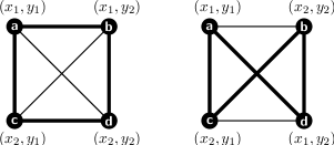
Figure 1: The edge $(a,b)$ is Cartesian in the left, and non-Cartesian in the right coordinatization

It is important to notice that although the PFD w.r.t. the strong product is unique, the coordinatizations might not be. Therefore, the assignment of an edge being Cartesian or non-Cartesian is not unique, in general. Figure 1 shows that the reason for the non-unique coordinatizations is the existence of automorphisms that interchange the vertices $b$ and $d$, but fix all the others. This is possible because $b$ and $d$ have the same 1-neighborhoods. Thus, an important issue in the context of strong graph products is whether or not two vertices can be distinguished by their neighborhoods. This is captured by the relation $S$ defined on the vertex set of $G$, which was first introduced by Dörfler and Imrich [3]. This relation is essential in the studies of the strong product.

Definition 2.2.

Let $G$ be a given graph and $x,y\in V(G)$ be arbitrary vertices. The vertices $x$ and $y$ are in relation $S$ if $N[x]=N[y]$. A graph is $S$-thin, or thin for short, if no two vertices are in relation $S$.

In [6], vertices $x$ and $y$ with $xSy$ are called interchangeable. Note that $xSy$ implies that $x$ and $y$ are adjacent since, by definition, $x\in N[x]$ and $y\in N[y]$. Clearly, $S$ is an equivalence relation. The graph $G/S$ is the usual quotient graph, more precisely, $G/S$ has vertex set $V(G/S)=\{S_{i}\mid S_{i}\text{ is an equivalence class of }S\text{ in }G\}$ and $(S_{i},S_{j})\in E(G/S)$ whenever $(x,y)\in E(G)$ for some $x\in S_{i}$ and $y\in S_{j}$.

Note that the relation $S$ on $G/S$ is trivial, that is, its equivalence classes are single vertices [24]. Thus $G/S$ is thin. The importance of thinness lies in the uniqueness of the coordinatizations, i.e., the property of an edge being Cartesian or not does not depend on the choice of the coordinates. As a consequence, the Cartesian edges are uniquely determined in an $S$-thin graph, see [3, 6].

Lemma 2.3.

If a graph $G$ is thin, then the set of Cartesian edges is uniquely determined and hence the coordinatization is unique.

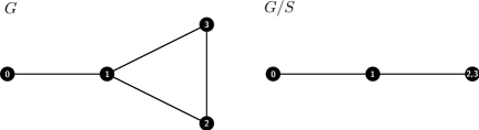
Figure 2: A graph $G$ and its quotient graph $G/S$. The S-classes are $S_{G}(0)=\{0\}$, $S_{G}(1)=\{1\}$, and $S_{G}(2)=S_{G}(3)=\{2,3\}$.

Another important basic property, first proved by Dörfler and Imrich [3], concerning the thinness of graphs is stated in the next lemma. Alternative proofs can be found in [24].

Lemma 2.4.

Let $S_{G}(v)$ denote the $S$-class in graph $G$ that contains vertex $v$. For any two graphs $G_{1}$ and $G_{2}$ holds $(G_{1}\boxtimes G_{2})/S\simeq G_{1}/S\boxtimes G_{2}/S$ and for every vertex $x=(x_{1},x_{2})\in V(G)$ holds $S_{G}(x)=S_{G_{1}}(x_{1})\times S_{G_{2}}(x_{2})$.
Thus, a graph is thin if and only if all of its factors with respect to the strong product are thin.

2.4 The Classical PFD Algorithm

In this subsection, we give a short overview of the classical PFD algorithm that is used locally later on.

The key idea of finding the PFD of a graph $G$ with respect to the strong product is to find the PFD of a subgraph $\mathbb{S}(G)$ of $G$, the so-called Cartesian skeleton, with respect to the Cartesian product and construct the prime factors of $G$ using the information of the PFD of $\mathbb{S}(G)$.

Definition 2.5.

A subgraph $H$ of a graph $G=G_{1}\boxtimes G_{2}$ with $V(H)=V(G)$ is called Cartesian skeleton of $G$, if it has a representation $H=H_{1}\Box H_{2}$ such that $V(H_{i}^{v})=V(G_{i}^{v})$ for all $v\in V(G)$ and $i\in\{1,2\}$. The Cartesian skeleton $H$ is denoted by $\mathbb{S}(G)$.

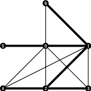
Figure 3: A prime graph $G$ and its Cartesian Skeleton $\mathbb{S}(G)$ induced by thick-lined edges. Thin-lined edges are marked as dispensable in the approach of Hammack and Imrich. On the other hand, the thick-lined edges are marked as Cartesian in the approach of Feigenbaum and Schäffer. However, in both cases the resulting Cartesian skeleton $\mathbb{S}(G)$ spans $G$. Hence, the vertex sets of the $\mathbb{S}(G)$-fiber (w.r.t. Cartesian product) and the $G$-fiber (w.r.t. strong product) induce the same partition $V(\mathbb{S}(G))=V(G)$ of the respective vertex sets.

In other words, the $H_{i}$-fibers of the Cartesian skeleton $\mathbb{S}(G)=H_{1}\Box H_{2}$ of a graph $G=G_{1}\boxtimes G_{2}$ induce the same partition as the $G_{i}$-fibers on the vertex sets $V(\mathbb{S}(G))=V(G)$. As Lemma 2.3 implies, if a graph $G$ is thin then the set of Cartesian edges and therefore $\mathbb{S}(G)$ is uniquely determined. The remaining question is: How can one determine $\mathbb{S}(G)$?

The first who answered this question were Feigenbaum and Schäffer [6]. In their polynomial-time approach, edges are marked as Cartesian if the neighborhoods of their endpoints fulfill some (strictly) maximal conditions in collections of neighborhoods or subsets of neighborhoods in $G$.

The latest and fastest approach for the detection of the Cartesian skeleton is due to Hammack and Imrich [9]. In distinction to the approach of Feigenbaum and Schäffer edges are marked as dispensable. All edges that are dispensable will be removed from $G$. The resulting graph $\mathbb{S}(G)$ is the desired Cartesian skeleton and will be decomposed with respect to the Cartesian product. For an example see Figure 3.

Definition 2.6.

An edge $(x,y)$ of $G$ is dispensable if there exists a vertex $z\in V(G)$ for which both of the following statements hold.

1. (a) $N[x]\cap N[y]\subset N[x]\cap N[z]$    or    (b) $N[x]\subset N[z]\subset N[y]$

2. (a) $N[x]\cap N[y]\subset N[y]\cap N[z]$   or   (b) $N[y]\subset N[z]\subset N[x]$

Some important results, concerning the Cartesian skeleton are summarized in the following theorem.

Theorem 2.7 ([9]).

Let $G=G_{1}\boxtimes G_{2}$ be a strong product graph. If $G$ is connected, then $\mathbb{S}(G)$ is connected. Moreover, if $G_{1}$ and $G_{2}$ are thin graphs then

$$\mathbb{S}(G_{1}\boxtimes G_{2})=\mathbb{S}(G_{1})\Box\mathbb{S}(G_{2}).$$

Any isomorphism $\varphi:G\rightarrow H$, as a map $V(G)\rightarrow V(H)$, is also an isomorphism $\varphi:\mathbb{S}(G)\rightarrow\mathbb{S}(H)$.

Remark 1.

Notice that the set of all Cartesian edges in a strong product $G=\boxtimes_{i=1}^{n}G_{i}$ of connected, thin prime graphs are uniquely determined and hence its Cartesian skeleton is. Moreover, since by Theorem 2.7 and Definition 2.5 of the Cartesian skeleton $\mathbb{S}(G)=\Box_{i=1}^{n}\mathbb{S}(G_{i})$ of $G$ we know that $V(\mathbb{S}(G)_{i}^{v})=V(G_{i}^{v})$ for all $v\in V(G)$. Thus, we can assume without loss of generality that the set of all Cartesian edges in a strong product $G=\boxtimes_{i=1}^{n}G_{i}$ of connected, thin graphs is the edge set of the Cartesian skeleton $\mathbb{S}(G)$ of $G$. As an example consider the graph $G$ in Figure 3. The edges of the Cartesian skeleton are highlighted by thick-lined edges and one can observe that not all edges of $G$ are determined as Cartesian. As it turns out $G$ is prime and hence, after the factorization of $\mathbb{S}(G)$, all edges of $G$ are determined as Cartesian belonging to a single factor.

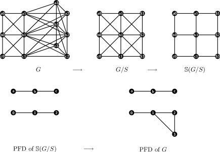
Figure 4: Illustrated are the basic steps of the PFD of strong product graphs.

Now, we are able to give a brief overview of the global approach that decomposes given graphs into their prime factors with respect to the strong product, see also Figure 4.

Given an arbitrary graph $G$, one first extracts a possible complete factor $K_{l}$ of maximal size, resulting in a graph $G^{\prime}$, i.e., $G\simeq G^{\prime}\boxtimes K_{l}$, and computes the quotient graph $H=G^{\prime}/S$. This graph $H$ is thin and therefore the Cartesian edges of $\mathbb{S}(H)$ can be uniquely determined. Now, one computes the prime factors of $\mathbb{S}(H)$ with respect to the Cartesian product and utilizes this information to determine the prime factors of $G^{\prime}$ by usage of an additional operation based on $gcd$’s of the size of the S-classes, see Lemma 5.40 and 5.41 provided in [24]. Notice that $G\simeq G^{\prime}\boxtimes K_{l}$. The prime factors of $G$ are then the prime factors of $G^{\prime}$ together with the complete factors $K_{p_{1}},\dots,K_{p_{j}}$, where $p_{1}\dots p_{j}$ are the prime factors of the integer $l$. Figure 4 gives an overview of the classical PFD algorithm.

One can bound the time complexity of this PFD algorithm as stated in the next Lemma, see [9] and [10].

Lemma 2.8 ([10]).

The PFD of a given graph $G$ with $n$ vertices and $m$ edges can be computed in $O(\max(mn\log n,m^{2}))$ time.

3 The Local Way to Go - Tools

As mentioned, we will utilize the classical PFD algorithm and derive a new approach for the PFD w.r.t. the strong product that makes only usage of small subgraphs, so-called subproducts of particular size, and that exploits the local information in order to derive the global factors. Moreover, motivated by the fact that most graphs are prime, although they can have a product-like structure, we want to vary this approach such that also disturbed products can be recognized. The key idea is the following: We try to cover a given disturbed product $G$ by subproducts that are itself ”undisturbed”. If the graph $G$ is not too much perturbed, we would expect to be able to cover most of it by factorizable $1$-neighborhoods or other small subproducts and to use this information for the construction of a strong product $H$ that approximates $G$.

However, for the realization of this idea several important tools are needed. First, we give an overview of the subproducts that will be used. We then introduce the so-called S1-condition, that is a property of an edge that allows us to determine Cartesian edges, even if the given graph is not thin. We continue to examine a subset of the vertex set of a given graph $G$, the so-called backbone $\mathbb{B}(G)$. Both concepts, the S1-condition and the backbone, have first been investigated in [14]. We will see that the backbone is closely related to the S1-condition. Finally, in order to identify locally determined fiber as belonging to one and the same or to different global factors, the so-called color-continuation property will be introduced. As it turns out, this particular property is not always met. Therefore, we continue to show how one can solve this problem for thin and later on for non-thin (sub)graphs.

3.1 Subproducts

In this subsection, we are concerned with so-called subproducts, also known as boxes [40], that will be used in the algorithm.

Definition 3.1.

A subproduct of a product $G\boxtimes H$, resp. $G\Box H$, is defined as the strong product, resp. the Cartesian product, of subgraphs of $G$ and $H$, respectively.

As shown in [13], it holds that $1$-neighborhoods in strong product graphs are subproducts:

Lemma 3.2 ([13]).

For any two graphs $G$ and $H$ holds $\langle N^{G\boxtimes H}[(x,y)]\rangle=\langle N^{G}[x]\rangle\boxtimes\langle N^{H}[y]\rangle$.

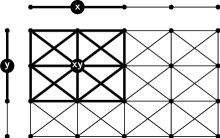
Figure 5: The 1-neighborhood $\langle N[(x,y)]\rangle=\langle N[x]\rangle\boxtimes\langle N[y]\rangle$ is highlighted by thick lined edges

For applications to approximate products it would be desirable to use small subproducts. Unfortunately, it turns out that 1-neighborhoods, which would be small enough for our purpose, are not sufficient to cover a given graph in general while providing enough information to recognize the global factors. However, we want to avoid to use 2-neighborhoods, although they are subproducts as well, they have diameter $4$ and are thus quite large. Therefore, we will define further small subgraphs, that are smaller than 2-neighborhoods, and show that they are also subproducts.

Definition 3.3.

Given a graph $G$ and an arbitrary edge $(v,w)\in E(G)$. The edge-neighborhood of $(v,w)$ is defined as

$$\langle N[v]\cup N[w]\rangle$$

and the $N^{*}_{v,w}$-neighborhood is defined as

$$N^{*}_{v,w}=\langle\bigcup_{x\in N[v]\cap N[w]}N[x]\rangle.$$

If there is no risk of confusion we will denote $N^{*}_{v,w}$-neighborhoods just by $N^{*}$-neighborhoods. We will show in the following that in addition to 1-neighborhoods also edge-neighborhoods of Cartesian edges and $N^{*}$-neighborhoods are subproducts and hence, natural candidates to cover a given graph as well. We show first, given a subproduct $H$ of $G$, that the subgraph which is induced by vertices contained in the union of 1-neighborhoods $N[v]$ with $v\in V(H)$, is itself a subproduct of $G$.

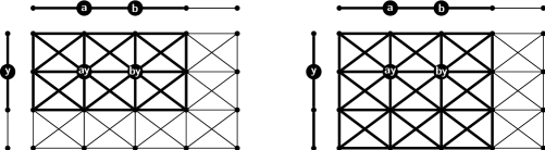
Figure 6: Shown is a strong product graph of two paths. Notice that the 2-neighborhood $\langle N_{2}[(b,y)]\rangle$ of vertex $(b,y)$ is isomorphic to $G$.
lhs.: The edge-neighborhood $\langle N[(a,y)]\cup N[(b,y)]\rangle=\langle(N[a]\cup N[b])\rangle\boxtimes\langle N[y]\rangle$.
rhs.: The $N^{*}$-neighborhood $N^{*}_{(a,y),(b,y)}=\langle\cup_{z\in N[a]\cap N[b]}N[z]\rangle\boxtimes\langle\cup_{z\in N[y]}N[z]\rangle$.

Lemma 3.4.

Let $G=G_{1}\boxtimes G_{2}$ be a strong product graph and $H=H_{1}\boxtimes H_{2}$ be a subproduct of $G$. Then

$$H^{*}=\left\langle\cup_{v\in V(H)}N^{G}[v]\right\rangle$$

is a subproduct of $G$ with $H^{*}=H_{1}^{*}\boxtimes H_{2}^{*}$, where $H_{i}^{*}$ is the induced subgraph of factor $G_{i}$ on the vertex set $V(H_{i}^{*})=\bigcup_{v_{i}\in V(H_{i})}N^{G_{i}}[v_{i}]$, $i=1,2$.

Proof.

It suffices to show that $V(H^{*})=V(H_{1}^{*})\times V(H_{2}^{*})$. For the sake of convenience, we denote $V(H_{i})$ by $V_{i}$, for $i=1,2$. We have: $V(H^{*})=\bigcup_{v\in V(H)}N^{G}[v]=\bigcup_{v\in V_{1}\times V_{2}}N^{G}[v].$

Since the induced neighborhood of each vertex $v=(v_{1},v_{2})$ in $G$ is the product of the corresponding neighborhoods $N^{G_{1}}[v_{1}]\boxtimes N^{G_{2}}[v_{2}]$ we can conclude:

$V(H^{*})=\bigcup_{\{v_{1}\in V_{1}\}\times\{v_{2}\in V_{2}\}}(N^{G_{1}}[v_{1}]\times N^{G_{2}}[v_{2}])=\bigcup_{v_{1}\in V_{1}}N^{G_{1}}[v_{1}]\times\bigcup_{v_{2}\in V_{2}}N^{G_{2}}[v_{2}]=V(H_{1}^{*})\times V(H_{2}^{*})$ ∎

Lemma 3.5.

Let $G$ be a nontrivial strong product graph and $(v,w)$ be an arbitrary edge of $G$. Then $\langle N^{G}[v]\cap N^{G}[w]\rangle$ is a subproduct.

Proof.

Let $v$ and $w$ have coordinates $(v_{1},v_{2})$ and $(w_{1},w_{2})$, respectively. Since $N^{G}[v]=N^{G_{1}}[v_{1}]\times N^{G_{2}}[v_{2}]$ we can conclude that $N^{G}[v]\cap N^{G}[w]=(N^{G_{1}}[v_{1}]\times N^{G_{2}}[v_{2}])\cap(N^{G_{1}}[w_{1}]\times N^{G_{2}}[w_{2}])=(N^{G_{1}}[v_{1}]\cap N^{G_{1}}[w_{1}])\times(N^{G_{2}}[v_{2}]\cap N^{G_{2}}[w_{2}]).$ ∎

Lemmas 3.2, 3.4 and 3.5 directly imply the next corollary.

Corollary 3.6.

Let $G$ be a given graph. Then for all $v\in V(G)$ and all edges $(v,w)\in E(G)$ holds:

$$\langle N_{2}[v]\rangle\text{ and }N^{*}_{v,w}$$

are subproducts of $G$. Moreover, if the edge $(v,w)$ is Cartesian than the edge-neighborhood

$$\langle N[v]\cup N[w]\rangle$$

is a subproduct of $G$.

Notice that $\langle N[v]\cup N[w]\rangle$ could be a product, i.e., not prime, even if $(v,w)$ is non-Cartesian in $G$. However, the edge-neighborhood of a single non-Cartesian edge is not a subproduct, in general. The obstacle we have is that a non-Cartesian edge of $G$ might be Cartesian in its edge-neighborhood. Therefore, we cannot use the information provided by the PFD of $\langle N[x]\cup N[y]\rangle$ to figure out if $(x,y)$ is Cartesian in $G$ and hence, if $\langle N[x]\cup N[y]\rangle$ is a proper subproduct. On the other hand, an edge that is Cartesian in a subproduct $H$ of $G$ must be Cartesian in $G$. To check if an edge $(x,y)$ is Cartesian in $\langle N[x]\cup N[y]\rangle$ that is Cartesian in $G$ as well we use the dispensable-property provided by Hammack and Imrich, see [9].

We show that an edge $(x,y)$ that is dispensable in $G$ is also dispensable in $\langle N[x]\cup N[y]\rangle$. Conversely, we can conclude that every edge that is indispensable in $\langle N[x]\cup N[y]\rangle$ must be indispensable and therefore Cartesian in $G$. This implies that every edge-neighborhood $\langle N[x]\cup N[y]\rangle$ is a proper subproduct of $G$ if $(x,y)$ is indispensable in $\langle N[x]\cup N[y]\rangle$.

Remark 2.

As mentioned in [9], we have:

• $N[x]\subset N[z]\subset N[y]$ implies $N[x]\cap N[y]\subset N[y]\cap N[z]$.

• $N[y]\subset N[z]\subset N[x]$ implies $N[x]\cap N[y]\subset N[x]\cap N[z]$.

• If $(x,y)$ is indispensable then $N[x]\cap N[y]\subset N[x]\cap N[z]$ and $N[x]\cap N[y]\subset N[y]\cap N[z]$ cannot both be true.

By simple set theoretical arguments one can easily prove the following lemma.

Lemma 3.7.

Let $(x,y)$ be an arbitrary edge of a given graph $G$ and $H=\langle N[x]\cup N[y]\rangle$. Then it holds:

$$N[x]\cap N[y]\subset N[x]\cap N[z]\Leftrightarrow N[x]\cap N[y]\cap H\subset N[x]\cap N[z]\cap H$$

and

$$N[x]\subset N[z]\subset N[y]\Rightarrow N[x]\cap H\subset N[z]\cap H\subset N[y]\cap H$$

Notice that the converse of the second statement does not hold in general, since $N[z]\cap H\subset N[y]\cap H=N[y]$ does not imply that $N[z]\subset N[y]$. However, by symmetry, Remark 2, Corollary 3.6, Lemma 3.7 we can conclude the next corollary.

Corollary 3.8.

If an edge $(x,y)$ of a thin strong product graph $G$ is indispensable in $\langle N[x]\cup N[y]\rangle$ and therefore Cartesian in $G$ then the edge-neighborhood $\langle N[x]\cup N[y]\rangle$ is a subproduct of $G$.

3.2 The S1-condition and the Backbone

The concepts of the S1-condition and the backbone were first introduced in [14]. The main idea of our approach is to construct the Cartesian skeleton of $G$ by considering PFDs of the introduced subproducts only. The main obstacle is that even though $G$ is thin, this is not necessarily true for subgraphs, Fig. 7. Hence, although the Cartesian edges are uniquely determined in $G$, they need not to be unique in those subgraphs. In order to investigate this issue in some more detail, we also define $S$-classes w.r.t. subgraphs $H$ of a given graph $G$.

Definition 3.9.

Let $H\subseteq G$ be an arbitrary induced subgraph of a given graph $G$. Then $S_{H}(x)$ is defined as the set

$$S_{H}(x)=\left\{v\in V(H)\mid N^{G}[v]\cap V(H)=N^{G}[x]\cap V(H)\right\}.$$

If $H=\langle N^{G}[y]\rangle$ for some $y\in V(G)$ we set $S_{y}(x):=S_{\langle N^{G}[y]\rangle}(x)$

In other words, $S_{H}(x)$ is the $S$-class that contains $x$ in the subgraph $H$. Notice that $N[x]\subseteq N[v]$ holds for all $v\in S_{x}(x)$. If $G$ is additionally thin, then $N[x]\subsetneq N[v]$.

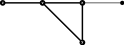
Figure 7: A thin graph where $\langle N[v]\rangle$ is not thin. The S-classes in $\langle N[v]\rangle$ are $S_{v}(v)=\{v\}$, $S_{v}(z)=\{z\}$ and $S_{v}(x)=S_{v}(y)=\{x,y\}$.

Since the Cartesian edges are globally uniquely defined in a thin graph, the challenge is to find a way to determine enough Cartesian edges from local information, even if $\langle N[v]\rangle$ is not thin. This will be captured by the S1-condition and the backbone of graphs.

Definition 3.10.

Given a graph $G$. An edge $(x,y)\in E(G)$ satisfies the S1-condition in an induced subgraph $H\subseteq G$ if

1. $x,y\in V(H)$ and

2. $|S_{H}(x)|=1$ or $|S_{H}(y)|=1$.

Note that $|S_{H}(x)|=1$ for all $x\in V(H)$, if $H$ is thin. From Lemma 2.4 we can directly infer that the cardinality of an $S$-class in a product graph $G$ is the product of the cardinalities of the corresponding $S$-classes in the factors. Applying this fact to subproducts of $G$ immediately implies Corollary 3.11.

Corollary 3.11.

Consider a strong product $G=\boxtimes_{i=1}^{n}G_{i}$ and a subproduct $H=\boxtimes_{i=1}^{n}H_{i}\subseteq G$. Let $x\in V(H)$ be a given vertex with coordinates $(x_{1},\dots,x_{n})$. Then $S_{H}(x)=\times_{i=1}^{n}S_{H_{i}}(x_{i})$ and therefore, $|S_{H}(x)|=\prod_{i=1}^{n}|S_{H_{i}}(x_{i})|$.

The most important property of Cartesian edges that satisfy the S1-condition in some quotient graph $G/S$ is that they can be identified as Cartesian edges in $G$, even if $G$ is not thin.

Lemma 3.12 ([14]).

Let $G=\boxtimes_{i=1}^{n}G_{i}$ be a strong product graph containing two S-classes $S_{G}(x)$, $S_{G}(y)$ that satisfy

1. $(S_{G}(x),S_{G}(y))$ is a Cartesian edge in $G/S$ and

2. $|S_{G}(x)|=1$ or $|S_{G}(y)|=1$.

Then all edges in G induced by vertices of $S_{G}(x)$ and $S_{G}(y)$ are Cartesian and copies of one and the same factor.

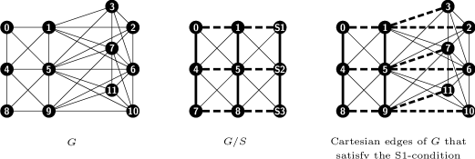
Figure 8: Determining Cartesian edges that satisfy the S1-condition. Given a graph $G$, one computes its quotient graph $G/S$. Since $G/S$ is thin the Cartesian edges of $G/S$ are uniquely determined. Now one factorizes $G/S$ and computes the prime factors of $G$. Apply Lemma 3.12 to identify all Cartesian edges with respective colors (thick and dashed lined) in $G$ that satisfy the S1-condition. The backbone $\mathbb{B}(G)$ is the singleton $\{5\}$.

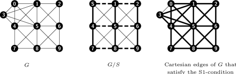
Figure 9: Determining Cartesian edges that satisfy the S1-condition. We factorize $G/S$ and compute the prime factors of $G$. Notice that it turns out that the factors induced by thick and dashed lined edges have to be merged to one factor. Apply now Lemma 3.12 to identify all Cartesian edges in $G$ that satisfy the S1-condition. In this case, it is clear that the edge $(0,3)$ has to be Cartesian as well and belongs to the single prime factor $G$. The backbone $\mathbb{B}(G)$ is the singleton $\{5\}$.

Remark 3.

Whenever we find a Cartesian edge $(x,y)$ in a subproduct $H$ of $G$ such that one endpoint of $(x,y)$ is contained in a $S$-class of cardinality $1$ in $H/S$, i.e., such that $S_{H}(x)=\{x\}$ or $S_{H}(y)=\{y\}$, we can therefore conclude that all edges in $H$ induced by vertices of $S_{H}(x)$ and $S_{H}(y)$ are also Cartesian and are copies of one and the same factor, see Figure 8.

Note, even if $H/S$ has more factors than $H$ the PFD algorithm provided by Imrich and Hammack indicates which factors have to be merged to one factor. Again we can conclude that all edges in $H$ that satisfy the S1-condition are Cartesian and are copies of one and the same factor, see Figure 9.

Moreover, since $H$ is a subproduct of $G$, it follows that any Cartesian edge of $H$ that satisfies the S1-condition is a Cartesian edge in $G$.

We consider now a subset of $V(G)$, the so-called backbone, which is essential for the algorithm.

Definition 3.13.

The backbone of a thin graph $G$ is the vertex set

$$\mathbb{B}(G)=\{v\in V(G)\mid|S_{v}(v)|=1\}\,.$$

Elements of $\mathbb{B}(G)$ are called backbone vertices.

Clearly, the backbone $\mathbb{B}(G)$ and the S1-condition are closely related, since all edges $(x,y)$ that contain a backbone vertex, say $x$, satisfy the S1-condition in $\langle N[x]\rangle$. If the backbone $\mathbb{B}(G)$ of a given graph $G$ is nonempty then Corollary 3.11 implies that no factor of $G$ is isomorphic to a complete graph, otherwise we would have $|S_{v}(v)|>1$ for all $v\in V(G)$. The last observations lead directly to the next corollary.

Corollary 3.14.

Given a graph $G$ with nonempty backbone $\mathbb{B}(G)$ then for all $v\in\mathbb{B}(G)$ holds: all edges $(v,x)\in E(\langle N[v]\rangle)$ satisfy the S1-condition in $N[v]$.

The set of backbone vertices of thin graphs can be characterized as follows.

Lemma 3.15 ([14]).

Let $G$ be a thin graph and $v$ an arbitrary vertex of $G$. Then $v\in\mathbb{B}(G)$ if and only if $N[v]$ is a strictly maximal neighborhood in $G$.

As shown in [14] the backbone B(G) of thin graphs G is a connected dominating set. This allows us to cover the entire graph by $1$-neighborhoods of the backbone vertices only. Moreover, it was shown that it suffices to exclusively use information about the $1$-neighborhood of backbone vertices, to find all Cartesian edges that satisfy the S1-condition in arbitrary $1$-neighborhoods, even those edges $(x,y)$ with $x,y\notin\mathbb{B}(G)$. These results are summarized in the next theorem.

Theorem 3.16 ([14]).

Let $G$ be a thin graph. Then the backbone $\mathbb{B}(G)$ is a connected dominating set for $G$.
All Cartesian edges that satisfy the S1-condition in an arbitrary induced 1-neighborhood also satisfy the S1-condition in the induced 1-neighborhood of a vertex of the backbone $\mathbb{B}(G)$.

Consider now the subproducts $\langle N[x]\rangle$, $N^{*}_{x,y}$ and $\langle N[x]\cup N[y]\rangle$ of a thin graph $G$. We will show in the following that the set of Cartesian edges of these subproducts that satisfy the S1-condition, induce a connected subgraph in the respective subproducts. This holds even if $\langle N[x]\rangle$, $N^{*}_{x,y}$ and $\langle N[x]\cup N[y]\rangle$ are not thin. For this we need the next lemmas.

Lemma 3.17.

Let G be a given thin graph, $x\in\mathbb{B}(G)$ and $H\subseteq G$ be an arbitrary induced subgraph such that $N[x]\subseteq V(H)$. Then $|S_{H}(x)|=1$ and $x\in\mathbb{B}(H)$.

Proof.

First notice that Lemma 3.15 and $x\in\mathbb{B}(G)$ implies that $\langle N[x]\rangle$ is strictly maximal in $G$. Since $\langle N[x]\rangle\subseteq H\subseteq G$ we can conclude that $\langle N[x]\rangle$ is strictly maximal in $H$. Hence, it holds $|S_{H}(x)|=1$. Moreover, it holds $|S_{x}(x)|=1$, otherwise there would be a vertex $y\in S_{x}(x),\ y\neq x$ and therefore, $N[x]\subseteq N[y]$. This contradicts that $\langle N[x]\rangle$ is strictly maximal in $H$. Hence, $x\in\mathbb{B}(H)$. ∎

Lemma 3.18.

Let $H=\boxtimes_{i=1}^{n}H_{i}$ be an arbitrary connected (not necessarily thin) graph and $(x,y)\in E(H)$ such that $|S_{H}(x)|=|S_{H}(y)|=1$. Then there is a path $\mathcal{P}_{x,y}$ from $x$ to $y$ consisting of Cartesian edges $(u,w)$ only with $|S_{H}(u)|=|S_{H}(w)|=1$.

Proof.

Let $(x,y)$ be an arbitrary edge of $H$ with $|S_{H}(x)|=|S_{H}(y)|=1$. From Corollary 3.11 we can conclude that $|S_{H_{i}}(x_{i})|=1$ and $|S_{H_{i}}(y_{i})|=1$ for all $i=1,\dots,n$. If $(x,y)$ is Cartesian there is nothing to show. Thus, assume $(x,y)$ is a non-Cartesian edge. Hence, the coordinates of $x=(x_{1},\dots,x_{n})$ and $y=(y_{1},\dots y_{n})$ differ in more than one position. W.l.o.g we assume that $x$ and $y$ differ in the first positions $1,\dots,k$. Hence $(x_{i},y_{i})\in E(G_{i})$ for all $i=1,\dots,k$ and $x_{i}=y_{i}$ for all $i=k+1,\dots,n$. Therefore, one can construct a path $\mathcal{P}_{x,y}$ with edge set $\{(y,v^{1}),(v^{1},v^{2}),\dots,(v^{k-1},x)\}$ such that the vertices $v^{j}$ have respective coordinates $(x_{1},x_{2},\dots,x_{j},y_{j+1},\dots,y_{n})$, $j=1,\dots,k-1$. Since all edges have endpoints differing in exactly one coordinate, all edges in $\mathcal{P}_{x,y}$ are Cartesian. Corollary 3.11 implies that for all those vertices hold $|S_{H}(v^{j})|=1$ and hence in particular for all edges $(u,w)\in\mathcal{P}_{x,y}$ hold $|S_{H}(u)|=1$ and $|S_{H}(w)|=1$. ∎

Lemma 3.19 ([14]).

Let $G$ be a thin, connected simple graph and $v\in V(G)$ with $|S_{v}(v)|>1$. Then there exists a vertex $y\in S_{v}(v)$ s.t. $|S_{y}(y)|=1$.

Lemma 3.20.

Let G be a given thin graph, $x,y\in\mathbb{B}(G)$ and let $H\subseteq G$ denote one of the subproducts $\langle N[x]\rangle$, $N^{*}_{x,y}$ or $\langle N[x]\cup N[y]\rangle$. In the latter case we assume that the edge $(x,y)$ is Cartesian in $H$. Then the set of all Cartesian edges of $H$ that satisfy the S1-condition in $H$ induce a connected subgraph of $H$.

Proof.

First, let $H=\langle N[x]\rangle$. Clearly, it holds $|S_{H}(x)|=1$. Let $(a,b)$ be an arbitrary edge that satisfy the S1-condition in $H$. W.l.o.g. we assume that $|S_{H}(a)|=1$. If $(a,x)$ is Cartesian there is nothing to show and if $(a,x)$ is non-Cartesian one can construct a path $\mathcal{P}_{x,a}$ as shown in Lemma 3.18.

Second, let $H=\langle N[x]\cup N[y]\rangle$. Lemma 3.17 implies that $|S_{H}(x)|=|S_{H}(y)|=1$. Let $(a,b)$ be an arbitrary edge that satisfy the S1-condition in $H$. W.l.o.g. we assume that $|S_{H}(a)|=1$. Moreover, let $a\in N[x]$. If $(a,x)$ is Cartesian there is nothing to show and if $(a,x)$ is non-Cartesian one can construct a path $\mathcal{P}_{x,a}$ as shown in Lemma 3.18. Analogously, one shows that such paths $\mathcal{P}_{y,a}$ can be constructed if $a\in N[y]$. Therefore, all Cartesian edges are connected to $x$ or $y$ via paths consisting of Cartesian edges only that satisfy the S1-condition. Furthermore $(x,y)$ is Cartesian and thus, the assertion follows for $H=\langle N[x]\cup N[y]\rangle$.

Third, let $H=N^{*}_{x,y}$. Lemma 3.17 implies that $|S_{H}(x)|=|S_{H}(y)|=1$. Therefore, one can construct a path $\mathcal{P}_{x,y}$ as shown in Lemma 3.18, since $(x,y)\in E(G)$. Let $(a,b)$ be an arbitrary edge that satisfy the S1-condition in $H$. W.l.o.g. we assume that $|S_{H}(a)|=1$. If $a\in N[x]$ or $a\in N[y]$ one can show by similar arguments as in the latter case that there is a path $\mathcal{P}_{x,a}$, resp., $\mathcal{P}_{y,a}$ consisting of Cartesian edges only that satisfy the S1-condition. Assume $a\notin N[x]$ and $a\notin N[y]$. Then there is a vertex $v\in N[x]\cap N[y]$ such that $a\in N[v]$. If $v\in\mathbb{B}(G)$ then Lemma 3.17 implies that $|S_{H}(v)|=1$, since $N[v]\subseteq V(H)$ and one construct a path $\mathcal{P}_{a,v}$ and $\mathcal{P}_{v,x}$ as in Lemma 3.18. Now assume $v\notin\mathbb{B}(G)$. Theorem 3.16 implies that there is a vertex $z\in\mathbb{B}(G)$ such that $z\in N[v]$. Moreover, as stated in Lemma 3.19, there exists even a vertex $z\in\mathbb{B}(G)$ such that $z\in S_{v}(v)$ and therefore $N[v]\cap N[z]=N[v]$. Thus it holds that $a,x,y\in N[z]$ and hence, $N[z]\subseteq H$. Therefore, Lemma 3.17 implies that $|S_{H}(z)|=1$. Analogously as in Lemma 3.18, one can construct a path $\mathcal{P}_{a,z}$ and $\mathcal{P}_{z,x}$, as well as a path $\mathcal{P}_{z,y}$ consisting of Cartesian edges only that satisfy the S1-condition. ∎

Last, we state two lemmas for later usage. Note, the second lemma refines the already known results of [14], where analogous results were stated for $2$-neighborhoods.

Lemma 3.21 ([14]).

Let $(x,y)\in E(G)$ be an arbitrary edge in a thin graph $G$ such that $|S_{x}(x)|>1$. Then there exists a vertex $z\in\mathbb{B}(G)$ s.t. $z\in N[x]\cap N[y]$.

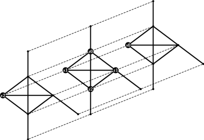
Figure 10: The Cartesian skeleton of the thin product graph $G$ of two prime factors induced by one connected component of thick and dashed lined edges. The backbone $\mathbb{B}(G)$ consists of the vertices $z_{1},z_{2}$ and $z_{3}$. In none of a edge-neighborhood $H$ holds $|S_{H}(x_{i})|=1$, $i=1,2,3$. Hence the fiber induced by vertices $x_{1},x_{2}$ and $x_{3}$ does not satisfy the S1-condition in any edge-neighborhood. To identify this particular fiber it is necessary to use $N^{*}$-neighborhoods. By Lemma 3.22 $N^{*}$-neighborhoods are also sufficient.

Lemma 3.22.

Let $G$ be a thin graph and $(v,w)$ be any edge of $G$. Let $N^{*}$ denote the $N^{*}_{v,w}$-neighborhood. Then it holds that $|S_{N^{*}}(v)|=1$ and $|S_{N^{*}}(w)|=1$ , i.e., the edge $(v,w)$ satisfies the S1-condition in $N^{*}$.

Proof.

Assume that $|S_{N^{*}}(v)|>1$. Thus there is a vertex $x\in S_{N^{*}}(v)$ different from $v$ with $N[x]\cap N^{*}=N[v]\cap N^{*}$, which implies that $w\in N[x]$ and hence, $x\in N[v]\cap N[w]$. Thus, it holds $N[x]\subseteq N^{*}$. Moreover, since $N[v]\subseteq N^{*}$ we can conclude that $N[v]=N[v]\cap N^{*}=N[x]\cap N^{*}=N[x]$, contradicting that $G$ is thin. Analogously, one shows that the statement holds for vertex $w$. ∎

3.3 The Color-Continuation

The concept of covering a graph by suitable subproducts and determining the global factors needs some additional improvements. Since we want to determine the global factors, we need to find their fibers. This implies that we have to identify different locally determined fibers as belonging to different or to one and the same global fiber. For this purpose, we formalize the term product coloring, color-continuation and combined coloring. Remind, the coordinatization of a product is equivalent to a (partial) edge coloring of $G$ in which edges $e=(x,y)$ share the same color $c(e)=k$ if $x$ and $y$ differ only in the value of a single coordinate $k$, i.e., if $x_{i}=y_{i}$, $i\neq k$ and $x_{k}\neq y_{k}$. This colors the Cartesian edges of $G$ (with respect to the given product representation).

Definition 3.23.

A product coloring of a strong product graph $G=\boxtimes_{i=1}^{n}G_{i}$ of $n\geq 1$ (not necessarily prime) factors is a mapping $P_{G}$ from a subset $E^{\prime}\subseteq E(G)$, that is a set of Cartesian edges of $G$, into a set $C=\{1,\dots,n\}$ of colors, such that all such edges in $G_{i}$-fibers obtain the same color $i$.

Definition 3.24.

A partial product coloring of a graph $G=\boxtimes_{i=1}^{n}G_{i}$ is a product coloring  that is only defined on edges that additionally satisfy the S1-condition in $G$.

Note, in a thin graph $G$ a product coloring and a partial product coloring coincide, since all edges satisfy the S1-condition in $G$.

Definition 3.25.

Let $H_{1},H_{2}\subseteq G$ and $P_{H_{1}}$, resp. $P_{H_{2}}$, be partial product colorings of $H_{1}$, resp. $H_{2}$. Then $P_{H_{2}}$ is a color-continuation of $P_{H_{1}}$ if for every color $c$ in the image of $P_{H_{2}}$ there is an edge in $H_{2}$ with color $c$ that is also in the domain of $P_{H_{1}}$.

The combined coloring on $H_{1}\cup H_{2}$ uses the colors of $P_{H_{1}}$ on $H_{1}$ and those of $P_{H_{2}}$ on $H_{2}\setminus H_{1}$.

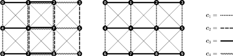
Figure 11: Shown is a thin graph $G$ with $\mathbb{B}(G)=\{x,y\}$. $G$ is the strong product of two paths. If one computes the PFD of the neighborhood $\langle N[x]\rangle$ one obtains a (partial) product coloring with colors $c_{1}$ and $c_{3}$. The (partial) product coloring of $\langle N[y]\rangle$ has colors $c_{2}$ and $c_{4}$. Since on edge $(x,y)$, resp. $(x,1)$, both colors $c_{1}$ and $c_{2}$, resp. $c_{3}$ and $c_{4}$ are represented we can identify those colors and merge them to one color, resulting in a proper combined coloring. Hence, the product coloring $P_{\langle N[x]\rangle}$ is a color-continuation of $P_{\langle N[y]\rangle}$ and vice versa.

In other words, for all newly colored edges with color $c$ in $H_{2}$, which are Cartesian edges in $H_{2}$ that satisfy the S1-condition in $H_{2}$, we have to find a representative edge that satisfy the S1-condition in $H_{1}$ and was already colored in $H_{1}$. If $H_{1}$ and $H_{2}$ are thin we can ignore the S1-condition, since all edges satisfy this condition in $H_{1}$ and $H_{2}$, see Figure 11.

However, there are cases where the color-continuation fails, see Figure 12. The remaining part of this subsection is organized as follows. We first show how one can solve the color-continuation problem if the corresponding subproducts are thin. As it turns out, it is sufficient to use the information of 1-neighborhoods only in order to get a proper combined coloring. We then proceed to solve this problem for non-thin subgraphs.

Before we continue, two important lemmas are given. The first one is just a restatement of a lemma, which was formulated for equivalence classes w.r.t. to a product relation in [27]. The second lemma shows how one can adapt this lemma to non-thin graphs.

Lemma 3.26 ([27], Lemma 1).

Let $G$ be a thin strong product graph and let $P_{G}$ be a product coloring of $G$. Then every vertex of $V(G)$ is incident to at least one edge with color $c$ for all colors $c$ in the image of $P_{G}$.

Lemma 3.27.

Let $G$ be a thin strong product graph, $H\subseteq G$ be a non-thin subproduct of $G$ and $x\in V(H)$ be a vertex with $|S_{H}(x)|=1$. Moreover, let $P_{H}$ be a partial product coloring of $H$. Then vertex $x$ is contained in at least one edge with color $c$ for all colors $c$ in the image of $P_{G}$.

Proof.

Notice that $H$ does not contain complete factors, otherwise Corollary 3.11 implies that $|S_{H}(x)|>1$. Now, the statement follows directly from Lemma 3.12 and Lemma 3.26 ∎

3.3.1 Solving the Color-Continuation Problem for Thin Subgraphs

To solve the color-continuation problem for thin subgraphs and in particular for thin 1-neighborhoods we introduce so-called S-prime graphs [12, 39, 34, 35, 33, 2, 21].

Definition 3.28.

A graph $S$ is S-prime (S stands for “subgraph”) if for all graphs $G$ and $H$ with $S\subseteq G\star H$ holds: $S\subseteq H$ or $S\subseteq G$, where $\star$ denotes an arbitrary graph product.

The class of S-prime graphs was introduced and characterized for the direct product by Sabidussi in 1975 [39]. Analogous notions of S-prime graphs with respect to other products are due to Lamprey and Barnes [34, 35]. Klavžar et al. [33] and Brešar [2] proved several characterizations of (basic) S-prime graphs. In [21] it is shown that so-called diagonalized Cartesian products of S-prime graphs are S-prime w.r.t. the Cartesian product. We shortly summarize the results of [21].

Definition 3.29 ([21]).

A graph $G$ is called a diagonalized Cartesian product, whenever there is an edge $(u,v)\in E(G)$ such that $H=G\setminus(u,v)$ is a nontrivial Cartesian product and $u$ and $v$ have maximal distance in $H$.

Theorem 3.30 ([21]).

The diagonalized Cartesian Product of S-prime graphs is S-prime w.r.t. the Cartesian product.

Corollary 3.31 ([21]).

Diagonalized Hamming graphs, and thus diagonalized Hypercubes, are S-prime w.r.t. the Cartesian product.

We shortly explain how S-prime graphs can be used in order to obtain a proper color-continuation in thin subproducts even if the color-continuation fails. Consider a strong product graph $G$ and two given thin subproducts $H_{1},H_{2}\subseteq G$. Let the Cartesian edges of each subgraph be colored with respect to a product coloring of $H_{1}$, respectively $H_{2}$ that is at least as fine as the product coloring of $G$ w.r.t. to its PFD. As stated in Definition 3.25, we have a proper color-continuation from $H_{1}$ to $H_{2}$ if for all colored edges with color $c$ in $H_{2}$ there is a representative edge that is colored in $H_{1}$. Assume the color-continuation fails, i.e., there is a color $c$ in $H_{2}$ such that for all edges $e_{c}\in E(H_{2})$ with color $c$ holds that $e_{c}$ is not colored in $H_{1}$, for an example see Figure 12. This implies that all such edges $e_{c}$ are determined as non-Cartesian in $H_{1}$. As claimed, the product colorings of $H_{1}$ and $H_{2}$ are at least as fine as the one of $G$ and $H_{1}$, $H_{2}$ are subproducts of $G$, which implies that colored Cartesian edges in each $H_{i}$ are Cartesian edges in $G$. Since $e_{c}$ is determined as non-Cartesian in $H_{1}$, but as Cartesian in $H_{2}$, we can infer that $e_{c}$ must be Cartesian in $G$. Thus we can force the edge $e_{c}$ to be Cartesian in $H_{1}$. The now arising questions is: ”What happens with the factorization of $H_{1}$?” We will show in the sequel that there is a hypercube in $H_{1}$ consisting of Cartesian edges only, where all edges are copies of edges of different factors. Furthermore, we show that this hypercube is diagonalized by a particular edge $e_{c}$ and therefore S-prime w.r.t the Cartesian product. Moreover, we will prove that all colors that appear on this hypercube and the color $c$ on $e_{c}$ have to be merged to exactly one color, even with respect to the product coloring, provided by the coloring w.r.t. the strong product. This approach solves the color-continuation problem for thin subproducts and hence in particular for thin 1-neighborhoods as well.

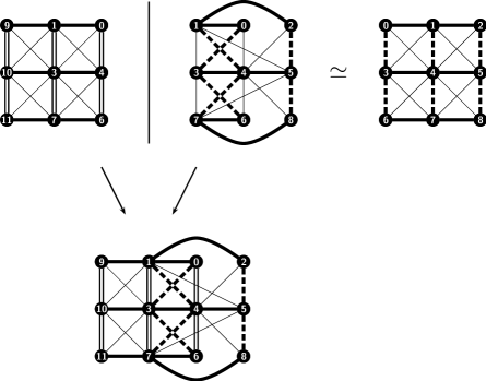
Figure 12: Color-continuation problem in thin subproducts. Consider the induced neighborhoods $\langle N[3]\rangle$ and $\langle N[4]\rangle$, depicted in the upper part. The colorings of the edges w.r.t. the PFD of each neighborhood are shown as thick dashed edges, thick-lined edges and double-lined edges, respectively. If we cover the graph $G$ in the lower part from $N[3]$ to $N[4]$ the color-continuation fails, e.g. on edge $(1,4)$, since $(1,4)$ is determined as non-Cartesian in $\langle N[3]\rangle$. This holds for all edges in $\langle N[3]\rangle$ that obtained the color ”thick dash” in $\langle N[3]\rangle$. The same holds for the color ”double-lined” if we cover the graph from $N[4]$ to $N[3]$. If we force the edge $(1,4)$ to be Cartesian in $\langle N[3]\rangle$ Lemma 3.33 implies that the colors ”thick-lined” and ”double-lined” have to be merged to one color, since the subgraph with edge set $\{(0,1),(0,4),(1,3),(3,4)\}\cup\{(1,4)\}$ is a diagonalized hypercube $Q_{2}$. Note, $G$ can be covered by thin 1-neighborhoods only, but the color-continuation fails. Hence $G$ is not NICE in the terminology of [13].

Lemma 3.32.

Let $G=\boxtimes_{l=1}^{n}G_{l}$ be a thin strong product graph and $(v,w)\in E(G)$ a non-Cartesian edge. Let $J$ denote the set of indices where $v$ and $w$ differ and $U\subseteq V(G)$ be the set of vertices $u$ with coordinates $u_{i}=v_{i}$, if $i\notin J$ and $u_{i}\in\{v_{i},w_{i}\}$, if $i\in J$. Then the induced subgraph $\langle U\rangle\subseteq\mathbb{S}(G)$ on $U$ consisting of Cartesian edges of $G$ only is a hypercube of dimension $|J|$.

Proof.

Notice that the coordinatization of $G$ is unique, since $G$ is thin. Moreover, since the strong product is commutative and associative we can assume w.l.o.g. that $J=\{1,\dots,k\}$. Note, that $k>1$, otherwise the edge $(v,w)$ would be Cartesian.

Assume that $k=2$. We denote the coordinates of $v$, resp. of $w$, by $(v_{1},v_{2},X)$, resp. by $(w_{1},w_{2},X)$. By definition of the strong product we can conclude that $(v_{i},w_{i})\in E(G_{i})$ for $i=1,2$. Thus the set of vertices with coordinates $(v_{1},v_{2},X)$ $(v_{1},w_{2},X)$,$(w_{1},v_{2},X)$, and $(w_{1},w_{2},X)$ induce a complete graph $K_{4}$ in $G$. Clearly, the subgraph consisting of Cartesian edges only is a $Q_{2}$.

Assume now the assumption is true for $k=m$. We have to show that the statement holds also for $k=m+1$. Let J={1,…,m+1} and let $U_{1}$ and $U_{2}$ be a partition of $U$ with $U_{1}=\{u\in U\mid u_{m+1}=v_{m+1}\}$ and $U_{2}=\{u\in U\mid u_{m+1}=w_{m+1}\}$. Thus each $U_{i}$ consists of vertices that differ only in the first $m$ coordinates. Notice, by definition of the strong product and by construction of both sets $U_{1}$ and $U_{2}$ there are vertices $a,b$ in each $U_{i}$ that differ in all $m$ coordinates that are adjacent in $G$ and hence non-Cartesian in $G$. Thus, by induction hypothesis the subgraphs $\langle U_{i}\rangle$ induced by each $U_{i}$ consisting of Cartesian edges only is a $Q_{m}$. Let $\langle U\rangle$ be the subgraph with vertex set $U$ and edge set $E(\langle U_{1}\rangle)\cup E(\langle U_{2}\rangle)\cup\{(a,b)\in E(G)\mid a=(X,v_{m+1},Y)$ and $b=(X,w_{m+1},Y)\}$. By definition of the strong product the edges $(a,b)$ with $a=(X,v_{m+1},Y)$ and $b=(X,w_{m+1},Y)$ induce an isomorphism between $\langle U_{1}\rangle$ and $\langle U_{2}\rangle$ which implies that $\langle U\rangle\simeq Q_{m}\Box K_{2}\simeq Q_{m+1}$. ∎

Lemma 3.33.

Let $G=\boxtimes_{l=1}^{n}G_{l}$ be a thin strong product graph, where each $G_{l}$, $l=1,\dots,n$ is prime. Let $H=\boxtimes_{l=1}^{m}H_{l}\subseteq G$ be a thin subproduct of $G$ such that there is a non-Cartesian edge $(v,w)\in E(H)$ that is Cartesian in $G$. Let $J$ denote the set of indices where $v$ and $w$ differ w.r.t. the coordinatization of $H$. Then the factor $\boxtimes_{i\in J}H_{i}$ of $H$ is a subgraph of a prime factor $G_{l}$ of $G$.

Proof.

In this proof, factors w.r.t. the Cartesian product and the strong product, respectively, are called Cartesian factors and strong factors, respectively. First notice that Cartesian edges in $G$ as well as in $H$ are uniquely determined, since both graphs are thin. Moreover, the existence of a Cartesian edge of $G=\boxtimes_{l=1}^{n}G_{l}$, that is a non-Cartesian edge in a subproduct $H=\boxtimes_{l=1}^{m}H_{l}$ of $G$, implies that $m>n$, i.e., the factorization of $H$ is a refinement of the factorization induced by the global PFD. Since $H$ is a thin subproduct of $G$ with a refined factorization, it follows that Cartesian edges of $H$ are Cartesian edges of $G$. Therefore, we can conclude that strong factors of $H$ are entirely contained in strong factors of $G$.

We denote the subgraph of $H$ that consists of all Cartesian edges of $H$ only, i.e., its Cartesian skeleton, by $\mathbb{S}(H)$, hence $\mathbb{S}(H)=\Box_{l=1}^{m}H_{l}$. Let $U\subseteq V(H)$ be the set of vertices $u$ with coordinates $u_{i}=v_{i}$, if $i\notin J$ and $u_{i}\in\{v_{i},w_{i}\}$, if $i\in J$. Notice that Lemma 3.32 implies that for the induced subgraph w.r.t. the Cartesian skeleton $\langle U\rangle\subseteq\mathbb{S}(H)$ holds $\langle U\rangle\simeq Q_{|J|}$. Moreover, the distance $d_{\langle U\rangle}(v,w)$ between $v$ and $w$ in $\langle U\rangle$ is $|J|$, that is the maximal distance that two vertices can have in $\langle U\rangle$. If we claim that $(v,w)$ has to be an edge in $\langle U\rangle$ we obtain a diagonalized hypercube $\langle U\rangle^{diag}$. Corollary 3.31 implies that $\langle U\rangle^{diag}$ is S-prime and hence $\langle U\rangle^{diag}$ must be contained entirely in a Cartesian factor $\widetilde{H}$ of a graph $H^{*}=\widetilde{H}\Box H^{\prime}$ with $\mathbb{S}(H)\cup(v,w)\subset H^{*}$. This implies that $\langle U\rangle^{diag}\subseteq\widetilde{H}^{u}$ for all $u\in V(H^{*})$, i.e., $\langle U\rangle^{diag}$ is entirely contained in all $\widetilde{H}^{u}$-layer in $H^{*}$. Note that all $\widetilde{H}$-layer $\widetilde{H}^{u}$ contain at least one edge of every $H_{i}$-layer $H_{i}^{u}$ of the previously determined factors $H_{i}$, $i\in J$ of $H$.

Furthermore, all Cartesian factors of $\mathbb{S}(H)=\Box_{l=1}^{m}H_{l}$ coincide with the strong factors of $H=\boxtimes_{l=1}^{m}H_{l}$ and hence, in particular the factors $H_{i},\ i\in J$. Moreover, since $H$ is a subproduct of $G$ and the factorization of $H$ is a refinement of $G$ it holds that Cartesian factors $H_{i},\ i\in J$ of $\mathbb{S}(H)$ must be entirely contained in strong prime factors of $G$. This implies that for all $i\in J$ the $H_{i}$-layer $H_{i}^{u}$ must be entirely contained in the layer of strong factors of $G$. We denote the set of all already determined strong factors $H_{i},\ i\in J$ of $H$ with $\mathcal{H}$.

Assume the graph $H^{*}=\Box_{j=1}^{s}K_{j}$ with $\mathbb{S}(H)\cup(v,w)\subseteq H^{*}$ and $V(H^{*})=V(\mathbb{S}(H))$ has a factorization such that $\Box_{i\in J}H_{i}\cup(v,w)\not\subseteq K_{j}$ for all Cartesian factors $K_{j}$. Since $\mathbb{S}(H)\cup(v,w)\subseteq H^{*}$, we can conclude that $\langle U\rangle^{diag}\subseteq H^{*}$. Since $\langle U\rangle^{diag}$ is S-prime it must be contained in a Cartesian factor $K_{r}$ of $H^{*}$. This implies that $\langle U\rangle^{diag}\subseteq K_{r}^{u}$ for all $u\in V(H^{*})$, i.e., for all $K_{r}$-layer of this particular Cartesian factor $K_{r}$. Since $\Box_{i\in J}H_{i}\cup(v,w)\not\subseteq K_{r}$, we can conclude that there is an already determined strong factor $H_{i}$ such that $H_{i}^{u}\not\subseteq K_{r}^{u}$ for all $u\in V(H^{*})$. Furthermore, all $K_{r}$-layer $K_{r}^{u}$ contain at least one edge of each $H_{i}$-layer $H_{i}^{u}$ of the previously determined strong factors $H_{i}$, $i\in J$ of $H$. We denote with $e$ the edge of the $H_{i}$-layer $H_{i}^{u}$ that is contained in the $K_{r}$-layer $K_{r}^{u}$. This edge $e$ cannot be contained in any $K_{j}$-layer, $j\neq r$. This implies that $H_{i}^{u}\not\subseteq K_{j}^{u}$ for any $K_{j}$-layer, $j=1,\dots,s$.

Thus, there is an already determined strong factor $H_{i}\in\mathcal{H}$ with $H_{i}^{u}\not\subseteq K_{j}^{u},\ u\in V(H^{*})$ for all $K_{j}$-layer in $H^{*}$, $j=1,\dots,s$. Therefore, none of the layer of this particular $H_{i}$ are subgraphs of layer of any Cartesian factor $K_{j}$ of $H^{*}$. This means that $H^{*}$ is not a subproduct of $G$ or a refinement of $H$, both cases contradict that $H_{i}\in\mathcal{H}$.

Therefore, we can conclude that $\langle U\rangle^{diag}\subseteq\Box_{i\in J}H_{i}\cup(v,w)\subseteq\widetilde{H}$ for a Cartesian factor $\widetilde{H}$ of $H^{*}$. As argued, Cartesian factors are subgraphs of its strong factors and hence, we can infer that $\Box_{i\in J}H_{i}$ and hence $\boxtimes_{i\in J}H_{i}$ must be entirely contained in a strong factor of $H$ and hence in a strong factor of $G$, since $H$ is a subproduct. ∎

3.3.2 Solving the Color-Continuation Problem for Non-Thin Subgraphs

The disadvantage of non-thin subgraphs is that, in contrast to thin subgraphs, not all edges satisfy the S1-condition. The main obstacle is that the color-continuation can fail if a particular color is represented on edges that don’t satisfy the S1-condition in any used subgraphs. Hence, those edges cannot be identified as Cartesian in the corresponding subgraphs, see Figure 13. Moreover, we cannot apply the approach that is developed for thin subgraphs by usage of diagonalized hypercubes in general. Therefore, we will extend 1-neighborhoods and use also edge- and $N^{*}$-neighborhoods.

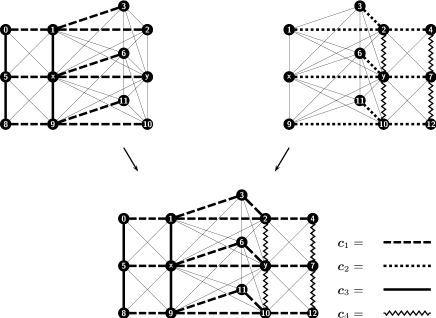
Figure 13: Color-continuation problem in non-thin subproducts. Shown is a thin graph $G$ that is a strong product of a path and a path containing a triangle. The backbone $\mathbb{B}(G)$ consists of the vertices $x$ and $y$. Both neighborhoods $\langle N[x]\rangle$ and $\langle N[y]\rangle$ are not thin. After computing the PFD of $\langle N[x]\rangle$, resp. of $\langle N[y]\rangle$ one obtains a partial product coloring with colors $c_{1}$ and $c_{3}$, resp. with colors $c_{2}$ and $c_{4}$. In this example the partial product coloring of $P_{\langle N[y]\rangle}$ is not a color-continuation of $P_{\langle N[x]\rangle}$ since no edge with color $c_{4}$ is colored in $\langle N[x]\rangle$.

In the following, we will provide several properties of (partial) product colorings and show that in a given thin strong product graph $G$ a partial product coloring $P_{H}$ of a subproduct $H\subseteq G$ is always a color-continuation of a partial product coloring $P_{\langle N[x]\rangle}$ of any 1-neighborhood $N[x]$ with $N[x]\subseteq V(H)$ and $x\in\mathbb{B}(G)$ and vice versa. This in turn implies that we always get a proper color-continuation from any 1-neighborhood $N[x]$ to edge-neighborhoods of edges $(x,y)$ and to $N^{*}_{x,y}$-neighborhoods with $y\in N[x]$ and vice versa.

Lemma 3.34.

Let $G$ be a thin graph and $x\in\mathbb{B}(G)$. Moreover let $P^{1}$ and $P^{2}$ be arbitrary partial product colorings of the induced neighborhood $\langle N[x]\rangle$.

Then $P^{2}$ is a color-continuation of $P^{1}$ and vice versa.

Proof.

Let $C^{1}$ and $C^{2}$ denote the images of $P^{1}$ and $P^{2}$, respectively. Note, the PFD of $\langle N[x]\rangle$ is the finest possible factorization, i.e., the number of used colors becomes maximal. Moreover, every fiber with respect to the PFD of $\langle N[x]\rangle$ that satisfies the S1-condition, is contained in any decomposition of $\langle N[x]\rangle$. In other words any prime fiber that satisfies the S1-condition is a subset of a fiber that satisfies the S1-condition with respect to any decomposition of $\langle N[x]\rangle$.

Moreover since $x\in\mathbb{B}(G)$ it holds that $|S_{x}(x)|=1$ and thus every edge containing vertex $x$ satisfies the S1-condition in $\langle N[x]\rangle$. Lemma 3.12 implies that all Cartesian edges $(x,v)$ can be determined as Cartesian in $\langle N[x]\rangle$. Together with Lemma 3.27 we can infer that each color of $C^{1}$, resp. $C^{2}$ is represented at least on edges $(x,v)$ contained in the prime fibers, which completes the proof. ∎

Lemma 3.35.

Let $G=\boxtimes_{i=1}^{n}G_{i}$ be a thin strong product graph. Furthermore let $H$ be a subproduct of $G$ with partial product coloring  $P_{H}$ and $\langle N[x]\rangle\subseteq H$ with $x\in\mathbb{B}(G)$.

Then $P_{H}$ is a color-continuation of the partial product coloring $P_{N}$ of $\langle N[x]\rangle$ and vice versa.

Proof.

First notice that Lemma 3.17 implies that $x\in\mathbb{B}(H)$ and in particular $|S_{H}(x)|=1$. Thus every edge containing vertex $x$ satisfies the S1-condition in $H$ as well as in $\langle N[x]\rangle$. Moreover, Lemma 3.27 implies that every color of the partial product coloring $P_{H}$, resp. $P_{N}$, is represented at least on edges $(x,v)$.

Since $\langle N[x]\rangle$ is a subproduct of the subproduct $H$ of $G$ we can conclude that the PFD of $H$ induces a local (not necessarily prime) decomposition of $\langle N[x]\rangle$ and hence a partial product coloring of $\langle N[x]\rangle$. Lemma 3.34 implies that any partial product coloring  of $\langle N[x]\rangle$ and hence in particular the one induced by $P_{H}$ is a color-continuation of $P_{N}$.

Conversely, any product coloring $P_{N}$ of $\langle N[x]\rangle$ is a color-continuation of the product coloring induced by the PFD of $\langle N[x]\rangle$. Since $\langle N[x]\rangle$ is a subproduct of $H$ it follows that every prime fiber of $\langle N[x]\rangle$ that satisfies the S1-condition is a subset of a prime fiber of $H$ that satisfies the S1-condition. This holds in particular for the fibers through vertex $x$, since $|S_{x}(x)|=1$ and $|S_{H}(x)|=1$. By the same arguments as in the proof of Lemma 3.34 one can infer that every product coloring of $H$ is a color-continuation of the product coloring induced by the PFD of $H$, which completes the proof. ∎

We can infer now the following Corollaries.

Corollary 3.36.

Let $G=\boxtimes_{i=1}^{n}G_{i}$ be a thin strong product graph, $(v,w)\in E(G)$ be a Cartesian edge of $G$ and $H$ denote the edge-neighborhood $\langle N[v]\cup N[w]\rangle$. Then any partial product coloring  $P_{H}$ of $H$ is a color-continuation of any partial product coloring $P_{N[v]}$ of $\langle N[v]\rangle$, resp. of any partial product coloring $P_{N[w]}$ of $\langle N[w]\rangle$ and vice versa.

Corollary 3.37.

Let $G=\boxtimes_{i=1}^{n}G_{i}$ be a thin strong product graph and $(v,w)\in E(G)$ be an arbitrary edge of $G$. Then any partial product coloring  $P^{*}$ of the $N^{*}_{v,w}$-neighborhood is a color-continuation of any partial product coloring $P_{N[v]}$ of $\langle N[v]\rangle$, resp. of any partial product coloring $P_{N[w]}$ of $\langle N[w]\rangle$ and vice versa.

4 A Local PFD Algorithm for Strong Product Graphs

In this section, we use the previous results and provide a general local approach for the PFD of thin graphs $G$. Notice that even if the given graph $G$ is not thin, the provided Algorithm works on $G/S$. The prime factors of $G$ can then be constructed by using the information of the prime factors of $G/S$ by repeated application of Lemma 5.40 provided in [24].

In this new PFD approach we use in addition an algorithm, called breadth-first search (BFS), that traverses all vertices of a graph $G=(V,E)$ in a particular order. We introduce the ordering of the vertices of $V$ by means of breadth-first search as follows: Select an arbitrary vertex $v\in V$ and create a sorted list $BFS(v)$ of vertices beginning with $v$; append all neighbors $v_{1},\ldots,v_{\deg(v)}$ of $v$; then append all neighbors of $v_{1}$ that are not already in this list; continue recursively with $v_{2},v_{3},\ldots$ until all vertices of $V$ are processed. In this way, we build levels where each $v$ in level $i$ is adjacent to some vertex $w$ in level $i-1$ and vertices $u$ in level $i+1$. We then call the vertex $w$ the parent of $v$ and vertex $v$ a child of $w$.

We give now an overview of the new approach. Its top level control structure is summarized in Algorithm 1.

Given an arbitrary thin graph $G$, first the backbone vertices are ordered via the breadth-first search (BFS). After this, the neighborhood of the first vertex $x$ from the ordered BFS-list $\mathbb{B}_{BFS}$ is decomposed. Then the next vertex $y\in N[x]\cap\mathbb{B}_{BFS}$ is taken and the edges of $\langle N[y]\rangle$ are colored with respect to the neighborhoods PFD. If the color-continuation from $\langle N[x]\rangle$ to $\langle N[y]\rangle$ does not fail, then the Algorithm proceeds with the next vertex $y^{\prime}\in N[x]\cap\mathbb{B}_{BFS}$. If the color-continuation fails and both neighborhoods are thin, one uses Algorithm 2 in order to compute a proper combined coloring. If one of the neighborhoods is non-thin the Algorithm proceeds with the edge-neighborhood $\langle N[x]\cup N[y]\rangle$. If it turns out that $(x,y)$ is indispensable in $\langle N[x]\cup N[y]\rangle$ and hence, that $\langle N[x]\cup N[y]\rangle$ is a proper subproduct (Corollary 3.8) the algorithm proceeds to decompose and to color $\langle N[x]\cup N[y]\rangle$. If it turns out that $(x,y)$ is dispensable in $\langle N[x]\cup N[y]\rangle$ the $N^{*}$-neighborhoods $N^{*}_{x,y}$ is factorized and colored. In all previous steps edges are marked as ”checked” if they satisfy the S1-condition, independent from being Cartesian or not. After this, the $N^{*}$-neighborhoods of all edges that do not satisfy the S1-condition in any of the previously used subproducts, i.e, 1-neighborhoods, edge-neighborhoods or $N^{*}$-neighborhoods, are decomposed and again the edges are colored. Examples of this approach are depicted in Figure 14 and 10. Finally, the Algorithm checks which of the recognized factors have to be merged into the prime factors $G_{1},\dots,G_{n}$ of $G$.

Algorithm 1 General Approach

1:  INPUT: a thin graph $G$

2:  compute backbone-vertices of $G$, order them in BFS and store them in $\mathbb{B}_{BFS}$;

3:  $x\leftarrow$ first vertex of $\mathbb{B}_{BFS}$;

4:  $W\leftarrow\{x\}$;

5:  FactorSubgraph($\langle N[x]\rangle$);

6:  while $\mathbb{B}_{BFS}\neq\emptyset$ do

7:     $H\leftarrow\langle\cup_{w\in W}N[w]\rangle$;

8:     for all $y\in N[x]\cap\mathbb{B}_{BFS}$ do

9:        FactorSubgraph($\langle N[y]\rangle$);

10:        compute the combined coloring of $H$ and $\langle N[y]\rangle$;

11:        if color-continuation fails from $H$ to $N[y]$ then

12:           if $\langle N[x]\rangle$ and $\langle N[y]\rangle$ are thin then

13:              $C\leftarrow\{\text{color }c\mid\text{color-continuation for }c\text{ fails}\}$;

14:              Solve-Color-Continuation-Problem(H, $\langle N[y]\rangle$, x, C); {Algorithm 2}

15:              mark all vertices and all edges of $\langle N[y]\rangle$ as ”checked”;

16:           else if (x,y) is indispensable in $\langle N[x]\cup N[y]\rangle$ then

17:              FactorSubgraph($\langle N[x]\cup N[y]\rangle$);

18:           else

19:              FactorSubgraph($N^{*}_{x,y}$);

20:           end if

21:           compute the combined coloring of $H$ and $\langle N[y]\rangle$;

22:        end if

23:     end for

24:     delete $x$ from $\mathbb{B}_{BFS}$;

25:     $x\leftarrow$ first vertex of $\mathbb{B}_{BFS}$;

26:     $W\leftarrow W\cup\{x\}$;

27:  end while

28:  while there exists a vertex $x\in V(H)$ that is not marked as ”checked” do

29:     if there exist edges $(x,y)$ that are not marked as ”checked” then

30:        FactorSubgraph($N^{*}_{x,y}$);

31:     else

32:        take an arbitrary edge $(x,y)\in E(H)$;

33:        FactorSubgraph($N^{*}_{x,y}$);

34:     end if

35:     compute the combined coloring of $H$ and $N^{*}_{x,y}$;

36:  end while

37:  for each edge $e\in E(H)$ do

38:     assign color of $e$ to edge $e\in E(G)$;

39:  end for

40:  CheckFactors(G); {check and merge factors with Algorithm 4}

41:  OUTPUT: G with colored $G_{j}$-fiber, and Factors of $G$;

Before we proceed to prove the correctness of this local PFD algorithm, we show that we always get a proper combined coloring by usage of Algorithm 2.

Lemma 4.1.

Let $G$ be a thin graph and $\mathbb{B}_{BFS}=\{v_{1},\dots,v_{n}\}$ be its BFS-ordered sequence of backbone vertices. Furthermore, let $H=\langle\cup_{j=1}^{i-1}N[v_{j}]\rangle$ be a partial product colored subgraph of $G$ that obtained its coloring from a proper combined product coloring induced by the PFD w.r.t. the strong product of each $\langle N[v_{j}]\rangle$, $j=1,\dots,i-1$. Let $\langle N[v_{i}]\rangle$ be a thin neighborhood that is product colored w.r.t. to its PFD. Let vertex $x$ denote the parent of $v_{i}$. Assume $\langle N[x]\rangle$ is thin. Moreover, assume the color-continuation from $H$ to $\langle N[v_{i}]\rangle$ fails and let $C$ denote the set of colors where it fails.

Then Algorithm 2 computes a proper combined coloring of the colorings of $H$ and $\langle N[v_{i}]\rangle$ with $H$, $\langle N[v_{i}]\rangle$, $x$ and $C$ as input.

Proof.

First notice that it holds $\langle N[x]\rangle\subseteq H=\langle\cup_{j=1}^{i-1}N[v_{j}]\rangle$. Let $c\in C$. Hence, $c$ denotes a color in $\langle N[v_{i}]\rangle$ such that for all edges $e\in E(\langle N[v_{i}]\rangle)$ with color $c$ holds that $e$ was not colored in $H$. Since the combined coloring in $H$ implies a product coloring of $\langle N[x]\rangle$ we can compute the coordinates of the vertices in $\langle N[x]\rangle$ with respect to this coloring. Notice that the coordinatization in $\langle N[x]\rangle$ is unique since $\langle N[x]\rangle$ is thin. Now Lemma 3.26 implies that there is at least one edge $e\in\langle N[v_{i}]\rangle$ with color $c$ that contains vertex $x$, since $x\in N[v_{i}]$. Let us denote this edge by $e_{c}=(x,w)$. Clearly, it holds $(x,w)\in E(\langle N[x]\rangle)$. Hence, this edge is not determined as Cartesian in $H$, and thus in particular not in $\langle N[x]\rangle$ otherwise $e_{c}$ would have been colored in $\langle N[x]\rangle$. But since $e_{c}$ is determined as Cartesian in $\langle N[v_{i}]\rangle$ and moreover, since $\langle N[v_{i}]\rangle$ is a subproduct of $G$, we can infer that $e_{c}$ must be Cartesian in $G$. Therefore, we claim that the non-Cartesian edge $(x,w)$ in $\langle N[x]\rangle$ has to be Cartesian in $\langle N[x]\rangle$. Notice that the product coloring of $\langle N[x]\rangle$ induced by the combined colorings of all $\langle N[v_{j}]\rangle$, $j=1,\dots,i-1$ is as least as fine as the product coloring of $G$. Thus, we can apply Lemma 3.33 and together with the unique coordinatization of $\langle N[x]\rangle$ directly conclude that all colors $k\in D$, where $D$ denotes the set of coordinates where $x$ and $w$ differ, have to be merged to one color. This implies that we always get a proper combined coloring and hence a proper color-continuation for each such color $c$ that is based on those additional edges $e_{c}=(x,w)$ as defined above. ∎

Algorithm 2 Solve-Color-Continuation-Problem

1:  INPUT: a partial product colored graph $H$, a product colored graph $\langle N[v_{i}]\rangle$, a vertex $v$, set $C$ of colors

2:  compute coordinates of $\langle N[v]\rangle$ with respect to the combined product coloring of $H$;

3:  {color ”j” if differ in coordinate ”j”}

4:  for all colors $c\in C$ {color-continuation fails} do

5:     take one representative $e_{c}=(v,w)\in E(\langle N[v_{i}]\rangle)$;

6:     $D\leftarrow\{k\mid v\text{ and }w\text{ differ in coordinate }k\}$;

7:     merge all colors $k\in D$ in $H$ to one color;

8:  end for

9:  compute the combined coloring of $H$ and $\langle N[v_{i}]\rangle$;

10:  OUTPUT: colored graph H, colored graph $\langle N[v_{i}]\rangle$;

Algorithm 3 FactorSubgraph

1:  INPUT: a graph $H$

2:  compute the PFD of $H$ and color the Cartesian edges in $H$ that satisfy the S1-condition;

3:  mark all vertices $x$ with $|S_{H}(x)|=1$ as ”checked”;

4:  mark all edges that satisfy the S1-condition as ”checked”;

5:  Return partially colored $H$;

Algorithm 4 CheckFactors

1:  INPUT: a thin product colored graph $G$

2:  take one connected component $G^{*}_{1},\dots,G^{*}_{l}$ of each color $1,\dots,l$ in $G$;

3:  $I\leftarrow\{1,\dots,l\}$;

4:  $J\leftarrow I$;

5:  for $k=1$ to $l$ do

6:     for each $S\subset J$ with $|S|=k$ do

7:        compute two connected components $A,\ A^{\prime}$ of $G$ induced by the colored edges of $G$ with color $i\in S,$ and $i\in I\backslash S$, resp;

8:        compute $H_{1}=\langle p_{A}(G)\rangle$ and $H_{2}=\langle p_{A^{\prime}}(G)\rangle$;

9:        if $H_{1}\boxtimes H_{2}\backsimeq G$ then

10:           save $H_{1}$ as prime factor;

11:           $J\leftarrow J\backslash S$;

12:        end if

13:     end for

14:  end for

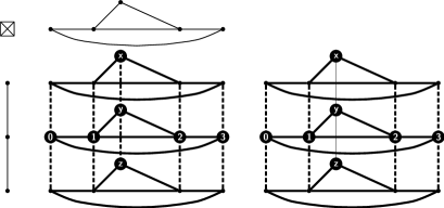
Figure 14: Depicted is the colored Cartesian skeleton of the thin strong product graph $G$ after running Algorithm 1 with different BFS-orderings $\mathbb{B}_{BFS}$ of the backbone vertices. The backbone $\mathbb{B}(G)$ consists of the vertices $0,1,2$ and $3$.
lhs.: $\mathbb{B}_{BFS}=2,1,3,0$. In this case the color-continuation from $N[2]$ to $N[1]$ fails. hence we compute the PFD of the edge-neighborhood $\langle N[2]\cup N[1]\rangle$. Notice that the Cartesian edges $(x,y)$ and $(y,z)$ satisfy the S1-condition in $\langle N[2]\cup N[1]\rangle$ and will be determined as Cartesian. In all other steps the color-continuation works.
rhs.: $\mathbb{B}_{BFS}=3,0,2,1$. In all cases ($N[3]$ to $N[0]$, $N[3]$ to $N[2]$, $N[0]$ to $N[1]$) the color-continuation works. However, after running the first while-loop there are missing Cartesian edges $(x,y)$ and $(y,z)$ that do not satisfy the S1-condition in any of the previously used subproducts $N[3]$, $N[0]$, $N[2]$ and $N[1]$. Moreover, the edge-neighborhoods $\langle N[x]\cup N[y]\rangle$ as well as $\langle N[z]\cup N[y]\rangle$ are the product of a path and a $K_{3}$ and the S1-condition is violated for the Cartesian edges in its edge-neighborhood. These edges will be determined in the second while-loop of Algorithm 1 using the respective $N^{*}$-neighborhoods.

Theorem 4.2.

Given a thin graph $G$ then Algorithm 1 determines the prime factors of $G$ with respect to the strong product.

Proof.

We have to show that every prime factor $G_{i}$ of $G$ is returned by our algorithm.

First, the algorithm scans all backbone vertices in their BFS-order stored in $\mathbb{B}_{BFS}$, which can be done, since $G$ is thin and hence, $\langle\mathbb{B}(G)\rangle$ is connected (Theorem 3.16).

In the first while-loop one starts with the first neighborhood $N[x]$ with $x$ as first vertex in $\mathbb{B}_{BFS}$, we proceed to cover the graph with neighborhoods $N[y]$ with $y\in\mathbb{B}_{BFS}$ and $y\in N[x]$. The following cases can occur:

1. If the color-continuation does not fail there is nothing to do. Furthermore, we can apply Lemma 3.20 and Lemma 3.27 and conclude that the determined Cartesian edges in $\langle N[x]\rangle$, resp. in $\langle N[y]\rangle$, i.e., the Cartesian edges that satisfy the S1-condition in $\langle N[x]\rangle$, resp. in $\langle N[y]\rangle$, induce a connected subgraph of $\langle N[x]\cup N[y]\rangle$.

2. If the color-continuation fails, we check if $\langle N[x]\rangle$ and $\langle N[y]\rangle$ are thin. If both neighborhoods are thin we can use Algorithm 2 to get a proper color-continuation from $\langle N[x]\rangle$ to $\langle N[y]\rangle$ (Lemma 4.1).

   Furthermore, since both neighborhoods are thin, for all vertices $v$ in $N[x]$, resp. $N[y]$, holds $|S_{x}(v)|=1$, resp. $|S_{y}(v)|=1$. Hence all edges in $\langle N[x]\rangle$, resp. $\langle N[y]\rangle$, satisfy the S1-condition. Therefore, by Lemma 3.20 the Cartesian edges span $\langle N[x]\rangle$ and $\langle N[y]\rangle$ and thus, by the color-continuation property, $\langle N[x]\cup N[y]\rangle$ as well.

3. If one of the neighborhoods is not thin then we check whether the edge $(x,y)$ is dispensable or not w.r.t. $\langle N[x]\cup N[y]\rangle$. If this edge is indispensable then Corollary 3.8 implies that $\langle N[x]\cup N[y]\rangle$ is a proper subproduct. Corollary 3.36 implies that then get a proper color-continuation from $\langle N[x]\cup N[y]\rangle$ to $\langle N[y]\rangle$.

   Furthermore, Lemma 3.17 implies that $|S_{\langle N[x]\cup N[y]\rangle}(x)|=1$. and $|S_{\langle N[x]\cup N[y]\rangle}(y)|=1$. From Lemma 3.20 we can conclude that the determined Cartesian edges of $\langle N[x]\cup N[y]\rangle$ induce a connected subgraph of $\langle N[x]\cup N[y]\rangle$.

4. Finally, if $(x,y)$ is dispensable in $\langle N[x]\cup N[y]\rangle$ we can not be assured that $\langle N[x]\cup N[y]\rangle$ is a proper subproduct. In this case we factorize $N^{*}_{x,y}$. Corollary 3.37 implies that we get a proper color-continuation from $N^{*}_{x,y}$ to $\langle N[y]\rangle$.

   Furthermore, Lemma 3.17 implies that $|S_{N^{*}_{x,y}}(x)|=1$ and $|S_{N^{*}_{x,y}}(y)|=1$. Moreover, from Lemma 3.20 follows that all Cartesian edges that satisfy the S1-condition on $N^{*}_{x,y}$ induce a connected subgraph of $N^{*}_{x,y}$.

Clearly, the previous four steps are valid for all consecutive backbone vertices $x,y\in\mathbb{B}_{BFS}$. Therefore, we always get a proper combined coloring of $H=\langle\cup_{w\in W}N[w]\rangle$ in Line 21, since $N[x]\subseteq H$ and hence, we always get a proper color-continuation from $H$ to $N[y]$. Furthermore, by this and the latter arguments in item $1.$–$4.$ concerning induced connected subgraphs we can furthermore conclude that all determined Cartesian edges induce a connected subgraph of $H=\langle\cup_{w\in\mathbb{B}(G)}N[w]\rangle$. The first while-loop will terminate since $\mathbb{B}_{BFS}$ is finite.

In all previous steps vertices $x$ are marked as ”checked” if there is a used subproduct $K$ such that $|S_{K}(x)|=1$. Edges are marked as ”checked” if they satisfy the S1-condition. Note, after the first while-loop has terminated either edges have been identified as Cartesian or if they have not been determined as Cartesian but satisfy the S1-condition they are at least connected to Cartesian edges that satisfy the S1-condition, which follows from Lemma 3.27. This implies that all edges that are marked as ”checked” are connected to Cartesian edges that satisfy the S1-condition. Moreover, notice that $H=\langle\cup_{w\in\mathbb{B}(G)}N[w]\rangle=G$, since $\mathbb{B}(G)$ is a dominating set.

In the second while-loop all vertices that are not marked as ”checked”, i.e., $|S_{K}(x)|>1$ for all used subproducts $K$, are treated. For all those vertices the $N^{*}$-neighborhoods $N^{*}_{x,y}$ are decomposed and colored. Lemma 3.22 implies that $|S_{N^{*}_{x,y}}(x)|=1$ and $|S_{N^{*}_{x,y}}(y)|=1$. Hence all Cartesian edges containing vertex $x$ or $y$ satisfy the S1-condition in $N^{*}_{x,y}$. Lemma 3.27 implies that each color of every factor of $N^{*}_{x,y}$ is represented on edges containing vertex $x$, resp., $y$. Lemma 3.20 implies that all Cartesian edges that satisfy the S1-condition in $N^{*}_{x,y}$ induce a connected subgraph of Lemma $N^{*}_{x,y}$.

It remains to show that we get always a proper color-continuation. Since $|S_{K}(x)|>1$ for all used subproducts $K$, we can conclude in particular that $|S_{x}(x)|>1$. Therefore, one can apply Lemma 3.21 and conclude that there exists a vertex $z\in\mathbb{B}(G)$ s.t. $z\in N[x]\cap N[y]$ and hence $\langle N[z]\rangle\subseteq N^{*}_{x,y}$. This neighborhood $\langle N[z]\rangle$ was already colored in one of the previous steps since $z\in\mathbb{B}(G)$. Lemma 3.17 implies that $|S_{N^{*}_{x,y}}(z)|=1$ and thus each color of each factor of $N^{*}_{x,y}$ is represented on edges containing vertex $z$ and all those edges can be determined as Cartesian via the S1-condition. We get a proper color-continuation from the already colored subgraph $H$ to $N^{*}_{x,y}$ since $N[z]\subseteq H$ and $N[z]\subseteq N^{*}_{x,y}$, which follows from Lemma 3.35 and Corollary 3.37.

The second while-loop will terminate since $V(H)$ is finite and $|S_{N^{*}_{x,y}}(x)|=1$ for all $x\in V(H)$.

As argued before, all edges that satisfy the S1-condition, which are all edges of $G$ after the second while-loop has terminated, are connected to Cartesian edges that satisfy the S1-condition. Moreover, all vertices have been marked as ”checked”. Hence, for all vertices holds $|S_{K}(x)|=1$ for some used subproduct $K$. Since we always got a proper combined coloring and hence, a proper color-continuation, we can apply Lemma 3.27, and conclude that the set of determined Cartesian edges induce a connected spanning subgraph $G$. Moreover, by the color-continuation property we can infer that the final number of colors on $G$ is at most the number of colors that were used in the first neighborhood. This number is at most $\log\Delta$, since every product of $k$ non-trivial factors must have at least $2^{k}$ vertices. Let’s say we have $l$ colors. As shown before, all vertices are ”checked” and thus we can conclude from Lemma 3.27 and the color-continuation property that each vertex $x\in V(G)$ is incident to an edge with color $c$ for all $c\in\{1,\dots,l\}$. Thus, we end with a combined coloring $F_{G}$ on $G$ where the domain of $F_{G}$ consists of all edges that were determined as Cartesian in the previously used subproducts.

It remains to verify which of the possible factors are prime factors of $G$. This task is done by using Algorithm 4. Clearly, for some subset $S\subset J$, $S$ will contain all colors that occur in a particular $G_{i}$-fiber $G_{i}^{a}$ which contains vertex $a$. Together with the latter arguments we can conclude that the set of $S$-colored edges in $G_{i}^{a}$ spans $G_{i}^{a}$. Since the global PFD induces a local decomposition, even if the used subproducts are not thin, every layer that satisfies the S1-condition in a used subproduct with respect to a local prime factor is a subset of a layer with respect to a global prime factor. Thus, we never identify colors that occur in copies of different global prime factors. In other words, the coloring $F_{G}$ is a refinement of the product coloring of the global PFD, i.e., it might happen that there are more colors than prime factors of $G$. This guarantees that a connected component of the graph induced by all edges with a color in $S$ induces a graph that is isomorphic to $G_{i}$. The same arguments show that the colors that are not in $S$ lead to the appropriate cofactor $H_{2}$. Thus $G_{i}$ will be recognized. ∎

Remark 4.

Algorithm 1 is a generalization of the results provided in [13, 14]. Hence, it computes the PFD of NICE [13] and locally unrefined [14] thin graphs. Moreover, even if we do not claim that the given graph $G$ is thin one can compute the PFD of arbitrary graphs $G$ as follows: We apply Algorithm 1 on $G/S$. The prime factors of $G$ can be constructed by using the information of the prime factors of $G/S$ and application of Lemma 5.40 provided in [24].

In the last part of this section, we show that Algorithm 1 computes the PFD with respect to the strong product of any connected thin graph $G$ in $O(|V|\cdot\Delta^{6})$ time. Clearly, this approach is not as fast as the approach of Hammack and Imrich, see Lemma 2.8, but it can easily be applied for the recognition of approximate products.

Theorem 4.3.

Given a thin graph $G=(V,E)$ with bounded maximum degree $\Delta$, then Algorithm 1 determines the prime factors of $G$ with respect to the strong product in $O(|V|\cdot\Delta^{7})$ time.

Proof.

For determining the backbone $\mathbb{B}(G)$ we have to check for a particular vertex $v\in V(G)$ whether there is a vertex $w\in N[v]$ with $N[w]\cap N[v]=N[v]$. This can be done in $O(\Delta^{2})$ time for a particular vertex $w$ in $N[v]$. Since this must be done for all vertices in $N[v]$ we end in time-complexity $O(\Delta^{3})$. This step must be repeated for all $|V|$ vertices of $G$. Hence, the time complexity for determining $\mathbb{B}(G)$ is $O(|V|\cdot\Delta^{3})$. Computing $\mathbb{B}_{BFS}$ via the breadth-first search takes $O(|V|+|E|)$ time. Since the number of edges is bounded by $|V|\cdot\Delta$ we can conclude that this task needs $O(|V|\cdot\Delta)$ time.

We consider now the Line 6 – 27 of the algorithm. The while-loop runs at most $|V|$ times. Computing $H$ in Line 7, i.e., adding a neighborhood to $H$, can be done in linear time in the number of edges of this neighborhood, that is in $O(\Delta^{2})$ time. The for-loop runs at most $\Delta$ times. Each neighborhood has at most $\Delta+1$ vertices and hence at most $(\Delta+1)\cdot\Delta$ edges. The PFD of $\langle N[y]\rangle$ can be computed in $O(\max(\Delta^{2}\Delta log(\Delta),\Delta^{4}))=O(\Delta^{4})$ time, see Lemma 2.8 The computation of the combined coloring of $H$ and $\langle N[y]\rangle$ can be done in constant time. For checking if the color-continuation is valid one has to check at most for all edges of $\langle N[v_{i}]\rangle$ if a respective colored edge was also colored in $H$, which can be done in $O(\Delta^{2})$ time.

Algorithm 2 computes the combined coloring of $H$ and $\langle N[v_{i}]\rangle$ in $O(\Delta^{2})$ time. To see this, notice that

1. the computation of the coordinates of the product colored neighborhood $\langle N[v]\rangle$ can be done via a breadth-first search in $\langle N[v]\rangle$ in $O(|N[v]|+|E(\langle N[v]\rangle)|)=O(\Delta+\Delta^{2})=O(\Delta^{2})$ time.

2. by the color-continuation property $H$ can have at most as many colors as there are colors for the first neighborhood $\langle N[v_{1}]\rangle$. This number is at most $\log(\Delta)$, because every product of $k$ non-trivial factors must have at least $2^{k}$ vertices. Thus the for-loop is repeated at most $\log(\Delta)$ times. All tasks in between the for-loop can be done in $O(\Delta)$ time and hence the for-loop takes $O(\log(\Delta)\cdot\Delta)$ time.

3. the computation the combined color can be done linear in the number of edges of $\langle N[v_{i}]\rangle$ and thus in $O(\Delta^{2})$ time.

It follows that all ”if” and ”else” conditions are bounded by the complexity of the PFD of the largest subgraph that is used and therefore by the complexity of the PFD of $N^{*}_{x,y}$.

Each $N^{*}$-neighborhood has at most $1+\Delta\cdot(\Delta-1)$ vertices. Therefore, the number of edges in each $N^{*}$-neighborhood is bounded by $(1+\Delta\cdot(\Delta-1))\cdot\Delta$. By Lemma 2.8 the computation of the PFD of each $N^{*}$ and hence, the assignment to an edge of being Cartesian is bounded by $O(\max(\Delta^{3}\Delta^{2}log(\Delta^{2}),\Delta^{6}))=O(\Delta^{6}).$

Since the while-loop (Line 6) runs at most $|V|$ times, the for-loop (Line 8) at most $\Delta$ times and the the time complexity for the PFD of the largest subgraph is $O(\Delta^{6})$, we end in an overall time complexity $O(|V|\Delta^{7})$ for the first part (Line 6 – 27) of the algorithm.

Using the same arguments, one shows that the time complexity of the second while-loop is $O(|V|\cdot\Delta^{6})$. The last for-loop (Line 37–39) needs $O(|E|)=O(|V|\cdot\Delta)$ time.

Finally, we have to consider Line 40 and therefore, the complexity of Algorithm 4. We observe that the size of $I$ is the number of used colors. As in the proof of Theorem 4.2, we can conclude that this number is bounded by $\log(\Delta)$. Hence, we also have at most $\Delta$ sets $S$, i.e., color combinations, to consider. In Line 7 of Algorithm 4 we have to find connected components of graphs and in Line 9 of Algorithm 4 we have to perform an isomorphism test for a fixed bijection. Both tasks take linear time in the number of edges of the graph and hence $O(|V|\cdot\Delta)$ time.

Considering all steps of Algorithm 1 we end in an overall time complexity $O(|V|\cdot\Delta^{7})$. ∎

5 Approximate Products

Finally, we show in this section, how Algorithm 1 can be modified and be used to recognize approximate products. For a formal definition of approximate graph products we begin with the definition of the distance between two graphs. We say the distance $d(G,H)$ between two graphs $G$ and $H$ is the smallest integer $k$ such that $G$ and $H$ have representations $G^{\prime}$, $H^{\prime}$ for which the sum of the symmetric differences between the vertex sets of the two graphs and between their edge sets is at most $k$. That is, if

$$|V(G^{\prime})\,\triangle\,V(H^{\prime})|+|E(G^{\prime})\,\triangle\,E(H^{\prime})|\leq k.$$

A graph $G$ is a $k$-approximate graph product if there is a product $H$ such that

$$d(G,H)\leq k.$$

As shown in [13] $k$-approximate graph products can be recognized in polynomial time.

Lemma 5.1 ([13]).

For fixed $k$ all strong and Cartesian $k$-approximate graph products can be recognized in polynomial time.

Without the restriction on $k$ the problem of finding a product of closest distance to a given graph $G$ is NP-complete for the Cartesian product. This has been shown by Feigenbaum and Haddad [5]. We conjecture that this also holds for the strong product. Moreover, we do not claim that the new algorithm for the recognition of approximate products finds an optimal solution in general, i.e., a product that has closest distance to the input graph. However, the given algorithm can be used to derive a suggestion of the product structure of given graphs and hence, of the structure of the global factors. For a more detailed discussion on how much perturbation is allowed such that the original factors or at least large factorizable subgraphs can still be recognized see Chapter 7 in [11].

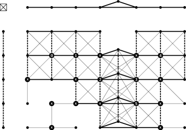
Figure 15: An approximate product $G$ of the product of a path and a path containing a triangle. The resulting colored graph after application of the modified Algorithm 1 is highlighted with thick and dashed edges. We set $P=1$, i.e., we do not use prime subproducts and hence only the vertices $0,1,\dots,5$ are used. Taking out one maximal component of each color would lead to appropriate approximate factors of $G$.

Let us start to explain this approach by an illustrating example. Consider the graph $G$ of Figure 15. It approximates $P_{5}\boxtimes P_{7}^{T}$, where $P_{7}^{T}$ denotes a path that contains a triangle. Suppose we are unaware of this fact. Clearly, if $G$ is non-prime, then every subproduct is also non-prime. We factorize every suitable subproduct of backbone vertices (1-neighborhood, edge-neighborhood, $N^{*}$-neighborhood) that is non-prime and try to use the information to find a product that is either identical to $G$ or approximates it. The backbone $\mathbb{B}(G)$ is a connected dominating set and consists of the vertices $0,1,\dots,5$ and all vertices marked with ”x”. The induced neighborhood of all ”x” marked vertices is prime. We do not use those neighborhoods, but the ones of the vertices $0,1,\ldots,5$, factorize their neighborhoods and consider the Cartesian edges that satisfy the S1-condition in the factorizations. There are two factors for every such neighborhood and thus, two colors for the Cartesian edges in every neighborhood. If two neighborhoods have a Cartesian edge that satisfy the S1-condition in common, we identify their colors. Notice that the color-continuation fails if we go from $\langle N[2]\rangle$ to $\langle N[3]\rangle$. Since the edge $(2,3)$ is indispensable in $\langle N[2]\cup N[3]\rangle$ and moreover, $\langle N[2]\cup N[3]\rangle$ is not prime, one factorizes this edge-neighborhood and get a proper color-continuation. In this way, we end up with two colors altogether, one for the horizontal Cartesian edges and one for the vertical ones. If $G$ is a product, then the edges of the same color span a subgraph with isomorphic components, that are either isomorphic to one and the same factor or that span isomorphic layers of one and the same factor. Clearly, the components are not isomorphic in our example. But, under the assumption that $G$ is an approximate graph product, we take one component for each color. In this example, it would be useful to take a component of maximal size, say the one consisting of the horizontal thick-lined edges through vertex $2$, and the vertical dashed-lined edges through vertex $3$. These components are isomorphic to the original factors $P_{5}$ and $P_{7}^{T}$. It is now easily seen that $G$ can be obtained from $P_{5}\boxtimes P_{7}^{T}$ by the deletion of edges. Other examples of recognized approximate products are shown in Figure 16 and 17.

As mentioned, Algorithm 1 has to be modified for the recognition of approximate products $G$. We summarize the modifications we apply:

1. $G/S$ is not computed. Hence, we do not claim that the given (disturbed) product is thin.

2. Item M1 and Theorem 3.16 imply that we cannot assume that the backbone is connected. Hence we only compute a BFS-ordering on connected components induced by backbone vertices.

3. We only use those subproducts (1-neighborhoods, edge-neighborhood, $N^{*}$-neighborhood) that have more than $P\geq 1$ prime factors, where $P$ is a fixed integer.

4. We do not apply the isomorphism test (line 40).

5. After coloring the graph, we take one minimal, maximal, or arbitrary connected component of each color. The choice of this component depends on the problem one wants to be solved.

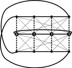
Figure 16: Shown is a prime graph $G$ with $\mathbb{B}(G)=\{0,1,2,3\}$. This kind of graph is also known as twisted product or graph bundle, see e.g. [26, 42]. In this example, each PFD of 1-neighborhoods leads to two factors. Notice that $G$ can be considered as an approximate product of a path $P_{3}$ and a cycle $C_{4}$. After application of the modified Algorithm 1 with $P=1$ we end with the given coloring (thick and dashed lines). Taking one minimal component of each color would lead to appropriate approximate factors of $G$.

Figure 17: An approximate product $G$ of the prime factors shown in Figure 15. In this example $G$ is not thin. Obviously, this graph seems to be less disturbed than the one in Figure 15. The thick vertices indicate the backbone vertices with more then $P=1$ prime factors. Application of the modified Algorithm 1 on $G$ (without computing $G/S$), choosing $P=1$ and using only the thick backbone vertices leads to a coloring with the four colors $c_{1},c_{2},c_{3}$ and $c_{4}$. This is due to the fact that the color-continuation fails, which would not be the case if we would allow to use also prime regions.

First, the quotient graph $G/S$ will not be computed, since the computation of $G/S$ of an approximate product graph $G$ may result in a thin graph where a lot of structural information has been lost.

Moreover, deleting or adding edges in a product graph $H$, resulting in a disturbed product graph $G$, usually makes the graph prime and also the neighborhoods $\langle N^{G}[v]\rangle$ that are different from $\langle N^{H}[v]\rangle$ and hence, the subproducts (edge-neighborhood, $N^{*}$-neighborhood) that contain $\langle N^{G}[v]\rangle$. In Algorithm 1, we therefore only use those subproducts of backbone vertices that are at least not prime, i.e., one restricts the set of allowed backbone vertices to those where the respective subproducts have more than $P\geq 1$ prime factors and thereby limiting the number of allowed subproducts. Hence, no prime regions or subproducts that have less or equal than $P$ prime factors are used. Therefore, one does not merge colors of different locally determined fibers to only $P$ colors, after the computation of a combined coloring.

The isomorphism test (line 40) in Algorithm 1 will not be applied. Thus, in prime graphs $G$ one does not merge colors if the product of the corresponding approximate prime factors is not isomorphic to $G$.

After coloring the graph, one takes out one component of each color to determine the (approximate) factors. For many kinds of approximate products the connected components of graphs induced by the edges in one component of each color will not be isomorphic. In the example in Figure 15, where the approximate product was obtained by deleting edges, it is easy to see that one should take the maximal connected component of each color.

Clearly, this approach needs non-prime subproducts. If most of the subgraphs in an approximate product $G$ are prime, one would not expect to obtain a product coloring of $G$, that can be used to recognize the original factors, but that can be used e.g. for determining maximal factorizable subgraphs or maximal subgraphs of fibers, see Chapter 7 in [11]. Hence, this approach may provide a basis for the development of further heuristics for the recognition of approximate products.

References

- [1] D. Archambault, T. Munzner, and D. Auber. TopoLayout: Multilevel graph layout by topological features. IEEE Trans. Vis. Comput. Graphics, 13(2):305–317, 2007.
- [2] B. Brešar. On subgraphs of Cartesian product graphs and S-primeness. Discrete Math., 282:43–52, 2004.
- [3] W. Dörfler and W. Imrich. Über das starke Produkt von endlichen Graphen. Österreih. Akad. Wiss., Mathem.-Natur. Kl., S.-B .II, 178:247–262, 1969.
- [4] J. Feigenbaum. Product graphs: some algorithmic and combinatorial results. Technical Report STAN-CS-86-1121, Stanford University, Computer Science, 1986. PhD Thesis.
- [5] J. Feigenbaum and R. A. Haddad. On factorable extensions and subgraphs of prime graphs. SIAM J. Discrete Math., 2:197–218, 1989.
- [6] J. Feigenbaum and A. A. Schäffer. Finding the prime factors of strong direct product graphs in polynomial time. Discrete Math., 109:77–102, 1992.
- [7] J. Hagauer and J. Žerovnik. An algorithm for the weak reconstruction of cartesian-product graphs. J. Combin. Inf. Syst. Sci., 24:97–103, 1999.
- [8] R. Hammack. On direct product cancellation of graphs. Discrete Math., 309(8):2538–2543, 2009.
- [9] R. Hammack and W. Imrich. On Cartesian skeletons of graphs. Ars Math. Contemp., 2(2):191–205, 2009.
- [10] R. Hammack, W. Imrich, and S Klavžar. Handbook of Product Graphs 2nd Edition. Discrete Math. Appl. CRC Press, 2011.
- [11] M. Hellmuth. Local Prime Factor Decomposition of Approximate Strong Product Graphs. PhD thesis, University Leipzig, Department of Mathematics and Computer Science, 2010.
- [12] M. Hellmuth. On the complexity of recognizing S-composite and S-prime graphs. Discr. Appl. Math., 161(7-8):1006 – 1013, 2013.
- [13] M. Hellmuth, W. Imrich, W. Klöckl, and P. F. Stadler. Approximate graph products. European J. Combin., 30:1119 – 1133, 2009.
- [14] M. Hellmuth, W. Imrich, W. Klöckl, and P. F. Stadler. Local algorithms for the prime factorization of strong product graphs. Math. Comput. Sci, 2(4):653–682, 2009.
- [15] M. Hellmuth, W. Imrich, and T. Kupka. Partial star products: A local covering approach for the recognition of approximate Cartesian product graphs. Math. Comput. Sci, 7(3):255–273, 2013.
- [16] M. Hellmuth, W. Imrich, and T. Kupka. Fast recognition of partial star products and quasi Cartesian products. Ars Math. Cont., 9(2):233 – 252, 2015.
- [17] M. Hellmuth and T. Marc. On the Cartesian skeleton and the factorization of the strong product of digraphs. J. Theor. Comp. Sci., 565(0):16–29, 2015.
- [18] M. Hellmuth, D. Merkle, and M. Middendorf. Extended shapes for the combinatorial design of RNA sequences. Int. J. of Computational Biology and Drug Design, 2(4):371–384, 2009.
- [19] M. Hellmuth, L. Ostermeier, and M. Noll. Strong products of hypergraphs: Unique prime factorization theorems and algorithms. Discr. Appl. Math., 171:60–71, 2014.
- [20] M. Hellmuth, L. Ostermeier, and P. F. Stadler. Unique square property, equitable partitions, and product-like graphs. Discr. Math., 320(0):92 – 103, 2014.
- [21] M. Hellmuth, L. Ostermeier, and P.F. Stadler. Diagonalized Cartesian products of S-prime graphs are S-prime. Discr. Math., 312(1):74 – 80, 2012.
- [22] M. Hellmuth, L. Ostermeier, and P.F. Stadler. A survey on hypergraph products. Math. Comput. Sci, 6:1–32, 2012.
- [23] M. Hellmuth, L Ostermeier, and P.F. Stadler. The relaxed square property. Australas. J. Combin., 62(3):240–270, 2015.
- [24] W. Imrich and S Klavžar. Product graphs. Wiley-Intersci. Ser. Discrete Math. Optim. Wiley-Interscience, New York, 2000.
- [25] W. Imrich, S. Klavžar, and F. R. Douglas. Topics in Graph Theory: Graphs and Their Cartesian Product. AK Peters, Ltd., Wellesley, MA, 2008.
- [26] W. Imrich, T. Pisanski, and J. Žerovnik. Recognizing cartesian graph bundles. Discr. Math, 167-168:393–403, 1997.
- [27] W. Imrich and J. Žerovnik. Factoring Cartesian-product graphs. J. Graph Theory, 18(6), 1994.
- [28] Wilfried Imrich and Janez Žerovnik. On the weak reconstruction of cartesian-product graphs. Discrete Math., 150(1-3), 1996.
- [29] Wilfried Imrich, Blaz Zmazek, and Janez Žerovnik. Weak k-reconstruction of cartesian product graphs. Electronic Notes in Discrete Mathematics, 10:297 – 300, 2001. Comb01, Euroconference on Combinatorics, Graph Theory and Applications.
- [30] Stefan Jänicke, Christian Heine, Marc Hellmuth, Peter F. Stadler, and Gerik Scheuermann. Visualization of graph products. IEEE Trans. Vis. Comput. Graphics, 16(6):1082–1089, 2010.
- [31] A. Kaveh and K. Koohestani. Graph products for configuration processing of space structures. Comput. Struct., 86(11-12):1219–1231, 2008.
- [32] A. Kaveh and H. Rahami. An efficient method for decomposition of regular structures using graph products. Intern. J. Numer. Meth. Eng., 61(11):1797–1808, 2004.
- [33] S. Klavžar, A. Lipovec, and M. Petkovšek. On subgraphs of Cartesian product graphs. Discrete Math., 244:223–230, 2002.
- [34] R. H. Lamprey and B. H. Barnes. A new concept of primeness in graphs. Networks, 11:279–284, 1981.
- [35] R. H. Lamprey and B. H. Barnes. A characterization of Cartesian-quasiprime graphs. Congr. Numer., 109:117–121, 1995.
- [36] R. McKenzie. Cardinal multiplication of structures with a reflexive relation. Fund. Math. LXX, pages 59–101, 1971.
- [37] P.J. Ostermeier, M. Hellmuth, K. Klemm, J. Leydold, and P.F. Stadler. A note on quasi-robust cycle bases. Ars Math. Contemp., 2(2):231–240, 2009.
- [38] G. Sabidussi. Graph multiplication. Mathematische Zeitschrift, 72:446–457, 1959.
- [39] G. Sabidussi. Subdirect representations of graphs in infinite and finite sets. Colloq. Math. Soc. Janos Bolyai, 10:1199–1226, 1975.
- [40] C. Tardif. A fixed box theorem for the Cartesian product of graphs and metric spaces. Discrete Math., 171(1-3):237–248, 1997.
- [41] V. G. Vizing. The Cartesian product of graphs. Vycisl. Sistemy, 9:30–43, 1963.
- [42] J. Žerovnik. On recognition of strong graph bundles. Math. Slovaca, 50:289–301, 2000.
- [43] G. Wagner and P. F. Stadler. Quasi-independence, homology and the unity of type: A topological theory of characters. J. Theor. Biol., 220:505–527, 2003.
- [44] B. Zmazek and J. Žerovnik. Algorithm for recognizing cartesian graph bundles. Discrete Appl. Math., 120:275–302, 2002.
- [45] B. Zmazek and J. Žerovnik. Weak reconstruction of strong product graphs. Discrete Math., 307:641–649, 2007.