Gradient recovery for elliptic interface problem: III. Nitsche’s method

Abstract

This is the third paper on the study of gradient recovery for elliptic interface problem. In our previous works [H. Guo and X. Yang, 2016, arXiv:1607.05898 and J. Comput. Phys., 338 (2017), 606–619], we developed gradient recovery methods for elliptic interface problem based on body-fitted meshes and immersed finite element methods. Despite the efficiency and accuracy that these methods bring to recover the gradient, there are still some cases in unfitted meshes where skinny triangles appear in the generated local body-fitted triangulation that destroy the accuracy of recovered gradient near the interface. In this paper, we propose a gradient recovery technique based on Nitsche’s method for elliptic interface problem, which avoids the loss of accuracy of gradient near the interface caused by skinny triangles. We analyze the supercloseness between the gradient of the numerical solution by the Nitsche’s method and the gradient of interpolation of the exact solution, which leads to the superconvergence of the proposed gradient recovery method. We also present several numerical examples to validate the theoretical results.

1 Introduction

Elliptic interface problems arise in many applications such as fluid dynamics and materials science, where the background consists of rather different materials on the subdomains separated by smooth curves called interface. The numerical challenge of interface problems comes from the fact that the solution, in general, has low global regularity due to the discontinuity of parameter (e.g. dielectric constant) at the interface. Standard finite element methods have been studied for elliptic interface problems by aligning the triangulation along the interface (body-fitted meshes), and are proven to achieve optimal convergence rates in both $L_{2}$ and energy norms [8, 3, 14, 54]. However, when the interface leads to subdomains of complex geometry, it is non-trivial and time-consuming to generate body-fitted meshes.

To overcome the difficulty of mesh generation in standard finite element method, tremendous effort has been input to develop numerical methods using unfitted (Cartesian) meshes. [49] is the first to propose the immersed boundary method (IBM) to simulate blood flow using Cartesian meshes. The idea of IBM is to use a Dirac $\delta$-function to model the discontinuity and discretize it to distribute a singular source to nearest grid points [49, 50]. But IBM only achieves the first-order accuracy. To improve the accuracy, Leveque and Li characterized the discontinuity as jump conditions and proposed the immersed interface method (IIM) [35]. IIM constructs special finite difference schemes to incorporate the jump conditions near the interface. High order unfitted finite difference methods including matched interface and boundary (MIB) method are also proposed in [60, 59]. We refer to [38] for a review on IIM and other unfitted finite difference methods.

In the meantime, unfitted numerical methods using finite element formulation are also developed for elliptic interface problems. The extended finite element method [7, 43, 19] enriches the standard continuous finite element space by adding some special basis functions to capture the discontinuity. The immersed finite element methods [36, 39, 40] modify the basis functions to satisfy the homogeneous jump conditions on interface elements. For the nonconforming immersed finite element method(IFEM) in [39], the numerical solution is continuous inside each element but can be discontinuous on the boundary of each element. Recently, there are also improved versions of IFEM such as the Petrov-Galerkin IFEM [30, 33, 31], symmetric and consistent IFEM [34], and partially penalized IFEM [42].

The Nitsche’s method [5, 11, 12, 10, 28, 25, 26, 27, 29], also called the cut finite element method, is firstly proposed by Hansbo and Hansbo in [25] to solve elliptic interface problems using unfitted meshes. It is further extended to deal with elastic problems with strong and weak discontinuities [26]. The study of the Nitsche’s method for Stokes interface problems can be found in [29]. The key idea of the Nitsche’s method is to construct an approximate solution on each fictitious domain and use Nitsche’s technique [48] to patch them together. A similar idea was used to develop the fictitious domain method [10, 11]. The robust forms of the unfitted Nitsche’s method were given in [2, 52]. The recent development of the cut finite element method is referred to the review paper [12].

For elliptic interface problems, computation of gradient plays an important role in many practical problems as discussed in [41], which demands numerical methods of high order accuracy. For standard elliptic problems, it is well known that the gradient recovery techniques [61, 63, 62, 57, 23, 1, 47, 46, 13, 55, 4] can reconstruct a highly accurate approximate gradient from the primarily computed data with reasonable cost. But for elliptic interface problems, only a few works have been done on the gradient recovery and associated superconvergence theory. For example in [53], a supercloseness result between the gradient of the linear finite element solution and the gradient of the linear interpolation is proved for a two-dimensional interface problem with a body-fitted mesh. For IFEM, Chou et al. introduced two special interpolation formulae to recover flux with high order accuracy for the one-dimensional linear and quadratic IFEM [15, 16]. Moreover, Li and his collaborators recently proposed an augmented immersed interface method [41] and a new finite element method [51] to accurately compute the gradient of the solution to elliptic interface problems. In our recent work [20], we proposed an improved polynomial preserving recovery for elliptic interface problems based on a body-fitted mesh and proved the superconvergence on both mildly unstructured meshes and adaptively refined meshes. Later in the two-dimensional case [21], we proposed gradient recovery methods based on symmetric and consistent IFEM [34] and Petrov-Galerkin IFEM [30, 32, 33] and numerically verified its superconvergence. In [24], we also provided a supercloseness result for the partially penalized IFEMs and proved that the recovered gradient using the gradient recovery method in [21] is superconvergent to the exact gradient.

Despite the efficiency and accuracy that the methods mentioned above bring to recover the gradient, there are still some cases in unfitted meshes where skinny triangles appear in the generated local body-fitted triangulation that destroy the accuracy of recovered gradient near the interface. In this paper, we propose an unfitted polynomial preserving recovery (UPPR) based on the Nitsche’s method. The key idea is to decompose the domain into two overlapping subdomains, named fictitious domains, by the interface and the triangulation proposed in the Nitsche’s method. On each fictitious domain, the standard linear finite element space will be used, and thus the classical polynomial preserving recovery (PPR) can be applied in each fictitious domain. Compared to previous gradient recovery methods [20, 21], the new method does not require generating a local body-fitted mesh and therefore avoids the drawback caused by skinny triangles. In general, the exact solutions of the interface problems are piecewise smooth on each subdomain. It implies that the extension of the exact solution on each subdomain to the whole domain is smooth, based on which, the recovered gradient using the interpolation of the exact solution is proven to be superconvergent to the exact gradient at rate of $\mathcal{O}(h^{2})$, and this is similar to the classical PPR for standard elliptic problems. In addition, we prove $\mathcal{O}(h^{1.5})$ supercloseness between the gradient given by the Nitsche’s method and the gradient of the interpolation of the exact solution by a sharp argument. This enables us to establish the complete superconvergence theory for the proposed UPPR.

The rest of the paper is organized as follows: We introduce briefly the elliptic interface problem and the Nitsche’s method in Section 2. In Section 3, we analyze the supercloseness for the Nitsche’s method and prove the $\mathcal{O}(h^{1.5})$ supercloseness between the gradient of the finite element solution and the gradient of the interpolation of the exact solution. In section 4, we describe the UPPR for the Nitsche’s method and establish its superconvergence theory. In Section 5, we present several numerical examples to confirm our theoretical results.

2 Nitsche’s method for elliptic interface problem

In this section, we first introduce the elliptic interface problem and associated notations, and then summarize the unfitted finite element discretization based on Nitsche’s method proposed in [2, 25] as a preparation for the unfitted polynomial preserving recovery (UPPR) method introduced later.

2.1 Elliptic interface problem

Let $\Omega$ be a bounded polygonal domain with Lipschitz boundary $\partial\Omega$ in $\mathbb{R}^{2}$. A $C^{2}$-curve $\Gamma$ divides $\Omega$ into two disjoint subdomains $\Omega_{1}$ and $\Omega_{2}$ as in Figure 1. We consider the following elliptic interface problem

$$-\nabla\cdot(\beta(z)\nabla u(z)) =f(z),\quad\text{ in }\Omega_{1}\cup\Omega_{2},$$ (2.1a)

$$u =0,\quad\quad\,\,\text{ on }\partial\Omega,$$ (2.1b)

$$\llbracket u\rrbracket =q,\quad\quad\,\,\text{ on }\Gamma$$ (2.1c)

$$\llbracket\beta\partial_{n}u\rrbracket =g,\quad\quad\,\,\text{ on }\Gamma$$ (2.1d)

where $\partial_{n}u=(\nabla u)\cdot n$ with $n$ being the unit outward normal vector of $\Gamma$ and the jump $\llbracket w\rrbracket$ on $\Gamma$ is defined as

$$\llbracket w\rrbracket=w_{1}-w_{2},$$ (2.2)

with $w_{i}=w|_{\Omega_{i}}$ being the restriction of $w$ on $\Omega_{i}$. The diffusion coefficient $\beta(z)\geq\beta_{0}$ is a piecewise smooth function, i.e.

$$\beta(z)=\left\{\begin{array}[]{ccc}\beta_{1}(z)&\text{if }z=(x,y)\in\Omega_{1},\\ \beta_{2}(z)&\text{if }z=(x,y)\in\Omega_{2},\\ \end{array}\right.$$ (2.3)

which has a finite jump of function value at the interface $\Gamma$.

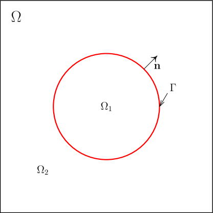
Figure 1: Typical example of domain $\Omega$ with interface $\Gamma$.

In this paper, we use the standard notations for Sobolev spaces and their associated norms as in [9, 17, 18]. For any bounded domain $D\subset\Omega$, the Sobolev space with norm $\|\cdot\|_{k,p,D}$ and seminorm $|\cdot|_{k,p,D}$ is denoted by $W^{k,p}(D)$. When $p=2$, $W^{k,2}(D)$ is simply denoted by $H^{k}(D)$ and the subscript $p$ is omitted in its associate norm and seminorm. Similar notations are applied to subdomains of $\Gamma$. Let $(\cdot,\cdot)_{D}$ and $\langle\cdot,\cdot\rangle_{\Gamma}$ denote the standard $L_{2}$ inner products of $L_{2}(D)$ and $L_{2}(\Gamma)$, respectively. For a bounded domain $D=D_{1}\cup D_{2}$ with $D_{1}\cap D_{2}=\emptyset$, let $W^{k,p}(D_{1}\cup D_{2})$ be the function space consisting of piecewise Sobolev functions $w$ such that $w|_{D_{1}}\in W^{k,p}(D_{1})$ and $w|_{D_{2}}\in W^{k,p}(D_{2})$, whose norm is defined as

$$\|w\|_{k,p,D_{1}\cup D_{2}}=\left(\|w\|_{k,p,D_{1}}^{p}+\|w\|_{k,p,D_{2}}^{p}\right)^{1/p},$$ (2.4)

and seminorm is defined as

$$|w|_{k,p,D_{1}\cup D_{2}}=\left(|w|_{k,p,D_{1}}^{p}+|w|_{k,p,D_{2}}^{p}\right)^{1/p}.$$ (2.5)

In this paper, we denote $C$ as a generic positive constant which can be different at different occurrences. In addition, it is independent of mesh size and the location of the interface.

2.2 Nitsche’s method

Let $\mathcal{T}_{h}$ be a triangulation of $\Omega$ independent of the location of the interface $\Gamma$. For any element $T\in\mathcal{T}_{h}$, let $h_{T}$ be the diameter of $T$ and $\rho_{T}$ be the diameter of the circle inscribed in $T$. In addition, we make the following assumptions on the triangulation.

Assumption 2.1.

The triangulation $\mathcal{T}_{h}$ is shape regular in the sense that there is a constant $\sigma$ such that

$$\frac{h_{T}}{\rho_{T}}\leq\sigma,$$ (2.6)

for any $T\in\mathcal{T}_{h}$.

Assumption 2.2.

The interface $\Gamma$ intersects each interface element boundary $\partial T$ exactly twice, and each open edge at most once.

To define the finite element space, denote the set of all elements that intersect the interface $\Gamma$ by

$$\mathcal{T}_{\Gamma,h}=\left\{T\in\mathcal{T}_{h}:\Gamma\cap\overline{T}\neq\emptyset\right\},$$ (2.7)

and denote the union of all such type elements by

$$\Omega_{\Gamma,h}=\bigcup\limits_{T\in\mathcal{T}_{\Gamma,h}}T.$$ (2.8)

Denote the set of all elements covering subdomain $\Omega_{i}$ to be

$$\mathcal{T}_{i,h}=\left\{T\in\mathcal{T}_{h}:\overline{\Omega_{i}}\cap\overline{T}\neq\emptyset\right\},\quad i=1,2;$$ (2.9)

and let

$$\Omega_{i,h}=\bigcup\limits_{T\in\mathcal{T}_{i,h}}T,\quad\omega_{i,h}=\bigcup\limits_{T\in\mathcal{T}_{i,h}\setminus\mathcal{T}_{\Gamma,h}}T,\quad i=1,2.$$ (2.10)

Figure 2 gives an illustration of $\Omega_{i,h}$ and $\omega_{i,h}$. We remark that $\Omega_{1,h}$ and $\Omega_{2,h}$ overlap on $\Omega_{\Gamma,h}$, which is shown as the shaded part in Figures 2b and 2c.

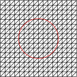
a

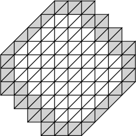
b

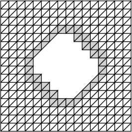
c

Figure 2: Triangulat $\mathcal{T}_{h}$ on the square domain $\Gamma$ with circular interface $\Gamma$. (a): Triangulation $\mathcal{T}_{h}$; (b): Triangulation $\mathcal{T}_{1,h}$ and $\omega_{1,h}$ (non-shaded triangles); (c): Triangulation $\mathcal{T}_{2,h}$ and $\omega_{2,h}$ (non-shaded triangles).

Let $V_{i,h}$ be the standard continuous linear finite element space on $\Omega_{i,h}$, i.e.

$$V_{i,h}=\left\{v\in C^{0}(\Omega_{i,h}):v|_{T}\in\mathbb{P}_{1}(T)\text{ for any }T\in\mathcal{T}_{i,h}\right\},\quad i=1,2,$$ (2.11)

where $\mathbb{P}_{1}(T)$ is the space of polynomials with degree $\leq 1$ on $T$. Then, we define the finite element space $V_{h}$ as

$$V_{h}=\left\{v_{h}=(v_{1,h},v_{2,h}):v_{i,h}\in V_{i,h},\,i=1,2\right\},$$ (2.12)

and $V_{h,0}$ as

$$V_{h,0}=\left\{v_{h}\in V_{h}:v_{h}|_{\partial\Omega}=0\right\}.$$ (2.13)

Note that a function in $V_{h}$ is a vector-valued function from $\mathbb{R}^{2}\mapsto\mathbb{R}^{2}$, which has a zero component in $\omega_{1,h}\bigcup\omega_{2,h}$ but in general two non-zero components in $\mathcal{T}_{\Gamma,h}$. It means that one will have two sets of basis functions for any element $T$ in $\mathcal{T}_{\Gamma,h}$: one for $V_{1,h}$ and the other for $V_{2,h}$.

For any $T$ in $\mathcal{T}_{\Gamma,h}$, denote $T_{i}=T\cap\Omega_{i}$ as the part of $T$ in $\Omega_{i}$, with $|T_{i}|$ being the measure of $T_{i}$ in $\mathbb{R}^{2}$. Denote $\Gamma_{T}=\Gamma\cap T$ as the part of $\Gamma$ in $T$, with $|\Gamma_{T}|$ being the measure of $\Gamma_{T}$ in $\mathbb{R}^{1}$. To increase the robustness of the Nitsche’s method, we introduce two weights as used in [2]

$$\kappa_{1}|_{T}=\frac{\beta_{2}|T_{1}|}{\beta_{2}|T_{1}|+\beta_{1}|T_{2}|},\quad\kappa_{2}|_{T}=\frac{\beta_{1}|T_{2}|}{\beta_{2}|T_{1}|+\beta_{1}|T_{2}|},$$ (2.14)

which satisfies that $\kappa_{1}+\kappa_{2}=1$. Then, we define the weighted averaging of a function $v_{h}$ in $V_{h}$ on the interface $\Gamma$ as

$$\{\kern-2.24998pt\{w\}\kern-2.24998pt\}=\kappa_{1}v_{1,h}+\kappa_{2}v_{2,h},\quad\{\kern-2.24998pt\{w\}\kern-2.24998pt\}^{\ast}=\kappa_{2}v_{1,h}+\kappa_{1}v_{2,h}.$$ (2.15)

Using the notations introduced above, the Nitsche’s method [12, 25, 2] for the elliptic interface problem (2.1) is to find $u_{h}\in V_{h,0}$ such that

$$a_{h}(u_{h},v_{h})=L_{h}(v_{h}),\quad\forall v_{h}\in V_{h,0};$$ (2.16)

where the bilinear form $a_{h}$ is defined as

$$\begin{split}a_{h}(u_{h},v_{h})=&\sum\limits_{i=1}^{2}\left(\beta\nabla u_{i,h},\nabla v_{i,h}\right)_{\Omega_{i}}-\left\langle\llbracket u_{h}\rrbracket,\{\kern-2.24998pt\{\beta\partial_{n}v_{h}\}\kern-2.24998pt\}\right\rangle_{\Gamma}\\ &-\left\langle\llbracket v_{h}\rrbracket,\{\kern-2.24998pt\{\beta\partial_{n}u_{h}\}\kern-2.24998pt\}\right\rangle_{\Gamma}+h^{-1}\left\langle\gamma\llbracket u_{h}\rrbracket,\llbracket v_{h}\rrbracket\right\rangle_{\Gamma},\end{split}$$ (2.17)

and the linear functional $L_{h}$ is defined as

$$L_{h}(v_{h})=\sum\limits_{i=1}^{2}(f,\nabla v_{i,h})_{\Omega_{i}}-\langle q,\{\kern-2.24998pt\{\beta\partial_{n}v_{h}\}\kern-2.24998pt\}\rangle_{\Gamma}+\left\langle\gamma q,\llbracket v_{h}\rrbracket,\right\rangle_{\Gamma}+\left\langle g,\{\kern-2.24998pt\{w\}\kern-2.24998pt\}^{\ast}\right\rangle_{\Gamma},$$ (2.18)

with the stability parameter

$$\gamma|_{T}=\frac{2h_{T}|\Gamma_{T}|}{|T_{1}|/\beta_{1}+|T_{2}|/\beta_{2}}.$$ (2.19)

In [2], the discrete variational form is shown to be consistent as the following theorem:

Theorem 2.3.

Let $u$ be the solution of the interface problem (2.1). Then we have

$$a_{h}(\tilde{u},v_{h})=L(v_{h}),\quad\forall v_{h}\in V_{h,0},$$ (2.20)

where $\tilde{u}=(u_{1},u_{2})$ with the short-hand notation $u_{i}=u|_{\Omega_{i}}$ as used in (2.2).

Theorem 2.3 implies the following Galerkin orthogonality:

Corollary 2.4.

Let $u$ be the solution of (2.1) and $u_{h}$ be the solution of the discrete problem (2.16). Then we have

$$a_{h}(\tilde{u}-u_{h},v_{h})=0,\quad\forall v_{h}\in V_{h,0},$$ (2.21)

with $\tilde{u}=(u_{1},u_{2})$.

To analyze the stability of the bilinear form $a_{h}(\cdot,\cdot)$, we introduce the following mesh-dependent norm [12, 25]

$$|||v|||_{h}^{2}=\|\nabla u\|_{0,\Omega_{1}\cup\Omega_{2}}^{2}+\sum\limits_{T\in\mathcal{T}_{\Gamma,h}}h_{T}\|\{\kern-2.24998pt\{\partial_{n}v\}\kern-2.24998pt\}\|_{0,\Gamma_{T}}^{2}+\sum\limits_{T\in\mathcal{T}_{\Gamma,h}}h_{T}^{-1}\|\llbracket v\rrbracket\|_{0,\Gamma_{T}}^{2}.$$ (2.22)

In [25], it is shown that the bilinear form $a_{h}(\cdot,\cdot)$ is coercive with respect to the above mesh-dependent norm in the following sense

Theorem 2.5.

There is a constant C such that

$$C|||v_{h}|||_{h}^{2}\leq a_{h}(v_{h},v_{h}),\quad\forall v_{h}\in V_{h}.$$ (2.23)

Based on the above coercivity, Hansbo et al. proved the following optimal convergence result [25]:

Theorem 2.6.

Let $u$ be the solution to the interface problem (2.1) and $u_{h}$ be the finite element solution to (2.16). If $u\in H^{2}(\Omega_{1}\cup\Omega_{2})$, then

$$|||\tilde{u}-u_{h}|||_{h}\leq Ch\|u\|_{2,\Omega_{1}\cup\Omega_{2}},$$ (2.24)

and

$$||\tilde{u}-u_{h}||_{0,\Omega}\leq Ch^{2}\|u\|_{2,\Omega_{1}\cup\Omega_{2}},$$ (2.25)

with $\tilde{u}=(u_{1},u_{2})$.

3 Supercloseness Analysis

In this section, we establish the supercloseness result between the gradient of the finite element solution and the gradient of the interpolation of the exact solution as a preparation for the superconvergence anaysis of the proposed gradient recovery technique based on Nitsche’s method. For that propose, we need the triangulation $\mathcal{T}_{h}$ to satisfy Condition $(\sigma,\alpha)$ as explained below.

Two adjacent triangles are said to form an $\mathcal{O}(h^{1+\alpha})$ approximate parallelogram if the lengths of any two opposite edges differ only by $\mathcal{O}(h^{1+\alpha})$.

Definition 3.1.

The triangulation $\mathcal{T}_{h}$ is called to satisfy Condition $(\sigma,\alpha)$ if there exist a partition $\mathcal{T}_{h}^{1}\cup\mathcal{T}_{h}^{2}$ of $\mathcal{T}_{h}$ and positive constants $\alpha$ and $\sigma$ such that every two adjacent triangles in $\mathcal{T}_{h}^{1}$ form an $\mathcal{O}(h^{1+\alpha})$ parallelogram and

$$\sum_{T\in{\mathcal{T}_{h}^{2}}}|T|=\mathcal{O}(h^{\sigma}).$$

Remark 3.1.

For the Nitsche’s method, we usually use a Cartesian mesh which is independent of the location of the interface. Therefore any Cartesian mesh satisfies Condition $(\sigma,\alpha)$ with $\sigma=\infty$ and $\alpha=1$.

To define the interpolation operator, we need to extend the function defined on the subdomain $\Omega_{i}$ to the whole domain $\Omega$. Let $E_{i}$, $i=1,2$, be the $H^{3}$-extension operator from $H^{3}(\Omega_{i})$ to $H^{3}(\Omega)$ such that

$$(E_{i}w)|_{\Omega_{i}}=w,$$ (3.1)

and

$$\|E_{i}w\|_{s,\Omega}\leq C\|w\|_{s,\Omega_{i}},\quad\forall w\in H^{s}(\Omega_{i}),\,s=0,1,2,3.$$ (3.2)

Let $I_{i,h}$ be the standard nodal interpolation operator from $C(\overline{\Omega})$ to $V_{i,h}$. Define the interpolation operator for the finite element space $V_{h}$ as

$$I_{h}^{\ast}v=(I_{1,h}^{\ast}v_{1},I_{1,h}^{\ast}v_{2}),$$ (3.3)

where

$$I_{i,h}^{\ast}=I_{i,h}E_{i}v_{i},\,i=1,2.$$ (3.4)

Optimal approximation capability of $I_{h}^{\ast}$ is proved in [25]. Assume $\mathcal{T}_{h}$ satisfies Condition $(\sigma,\alpha)$, and then we can prove the following theorem:

Theorem 3.2.

Suppose the triangulation $\mathcal{T}_{h}$ satisfies Condition $(\sigma,\alpha)$. Let $u$ be the solution of the interface problem (2.1) and $I_{h}^{\ast}u$ be the interpolation of $u$ in the finite element space $V_{h,0}$. If $u\in H^{1}(\Omega)\cap H^{3}(\Omega^{-}\cup\Omega^{+})\cap W^{2,\infty}(\Omega^{-}\cup\Omega^{+})$, then for $\tilde{u}=(u_{1},u_{2})$ and all $v_{h}\in V_{h,0}$,

$$a_{h}(\tilde{u}-I_{h}^{\ast}u,v_{h})\leq C\biggl{(}h^{1+\rho}(\|u\|_{3,\Omega^{+}\cup\Omega^{-}}+\|u\|_{2,\infty,\Omega^{+}\cup\Omega^{-}})\\ +Ch^{3/2}\|u\|_{2,\infty,\Omega^{+}\cup\Omega^{-}}\biggr{)}|v_{h}|_{h}.$$ (3.5)

where $\rho=\min(\alpha,\frac{\sigma}{2},\frac{1}{2})$.

Proof.

By (2.17), we have

$$a_{h}(\tilde{u}-I_{h}^{\ast}u,v_{h})$$ (3.6)

$$= \sum\limits_{i=1}^{2}\left(\beta\nabla(u_{i}-I_{i,h}^{\ast}u_{i}),\nabla v_{i,h}\right)_{\Omega_{i}}-\left\langle\llbracket u-I_{h}^{\ast}u\rrbracket,\{\kern-2.24998pt\{\beta\partial_{n}v_{h}\}\kern-2.24998pt\}\right\rangle_{\Gamma}$$

$$-\left\langle\llbracket v_{h}\rrbracket,\{\kern-2.24998pt\{\beta\partial_{n}(u-I_{h}^{\ast}u)\}\kern-2.24998pt\}\right\rangle_{\Gamma}+h^{-1}\left\langle\gamma\llbracket u-I_{h}^{\ast}u\rrbracket,\llbracket v_{h}\rrbracket\right\rangle_{\Gamma}$$

$$= \left(\beta\nabla(u_{1}-I_{1,h}^{\ast}u_{1}),\nabla v_{1,h}\right)_{\omega_{1,h}}+\left(\beta\nabla(u_{2}-I_{2,h}^{\ast}u_{2}),\nabla v_{2,h}\right)_{\omega_{2,h}}$$

$$+\left(\beta\nabla(u-I_{h}^{\ast}u),\nabla v_{h}u\right)_{\Omega_{\Gamma,h}}-\left\langle\llbracket u-I_{h}^{\ast}u\rrbracket,\{\kern-2.24998pt\{\beta\partial_{n}v_{h}\}\kern-2.24998pt\}\right\rangle_{\Gamma}$$

$$-\left\langle\llbracket v_{h}\rrbracket,\{\kern-2.24998pt\{\beta\partial_{n}(u-I_{h}^{\ast}u)\}\kern-2.24998pt\}\right\rangle_{\Gamma}+h^{-1}\left\langle\gamma\llbracket u-I_{h}^{\ast}u\rrbracket,\llbracket v_{h}\rrbracket\right\rangle_{\Gamma}$$

$$:= F_{1}+F_{2}+F_{3}+F_{4}+F_{5}+F_{6}.$$

Since $\mathcal{T}_{h}$ satisfies Condition $(\sigma,\alpha)$, it follows that $\mathcal{T}_{1,h}\setminus\mathcal{T}_{\Gamma,h}$ and $\mathcal{T}_{2,h}\setminus\mathcal{T}_{\Gamma,h}$also satisfy Condition $(\sigma,\alpha)$. Notice that the restriction of the finite element space $V_{i,h}$ on $\omega_{i,h}$ is just the standard continuous linear finite element space for $i=1,2$. Then by Lemma $2.1$ in [55], we have

$$|F_{1}|\leq Ch^{1+\rho}(\|u\|_{3,\Omega_{1}}+\|u\|_{2,\infty,\Omega_{1}})|v_{h}|_{h},$$ (3.7)

$$|F_{2}|\leq Ch^{1+\rho}(\|u\|_{3,\Omega_{2}}+\|u\|_{2,\infty,\Omega_{2}})|v_{h}|_{h},$$ (3.8)

where $\rho=\min(\alpha,\frac{\sigma}{2},\frac{1}{2})$. To estimate $I_{3}$, the Cauchy-Schwartz inequality implies

$$F_{3}\leq C_{1}\left(\sum_{T\in\mathcal{T}_{\Gamma,h}}\|\nabla(u_{1}-I_{1,h}^{\ast}u_{1})\|_{0,T_{1}}^{2}\right)^{1/2}\left(\sum_{T\in\mathcal{T}_{\Gamma,h}}\|\nabla v_{1,h}\|_{0,T_{1}}^{2}\right)^{1/2}$$

$$+C_{2}\left(\sum_{T\in\mathcal{T}_{\Gamma,h}}\|\nabla(u_{2}-I_{1,h}^{\ast}u_{2})\|_{0,T_{2}}^{2}\right)^{1/2}\left(\sum_{T\in\mathcal{T}_{\Gamma,h}}\|\nabla v_{2,h}\|_{0,T_{2}}^{2}\right)^{1/2}$$

$$\leq C_{1}\left(\sum_{T\in\mathcal{T}_{\Gamma,h}}h^{4}\|u\|_{2,\infty,\Omega_{1}}^{2}\right)^{1/2}\left(\sum_{T\in\mathcal{T}_{\Gamma,h}}\|\nabla v_{1,h}\|_{0,T_{1}}^{2}\right)^{1/2}$$

$$+C_{2}\left(\sum_{T\in\mathcal{T}_{\Gamma,h}}h^{4}\|u\|_{2,\infty,\Omega_{2}}^{2}\right)^{1/2}\left(\sum_{T\in\mathcal{T}_{\Gamma,h}}\|\nabla v_{2,h}\|_{0,T_{2}}^{2}\right)^{1/2}$$

$$\leq C_{1}h^{2}\|u\|_{2,\infty,\Omega_{1}}\left(\sum_{T\in\mathcal{T}_{\Gamma,h}}1\right)^{1/2}\left(\sum_{T\in\mathcal{T}_{\Gamma,h}}\|\nabla v_{1,h}\|_{0,T_{1}}^{2}\right)^{1/2}$$

$$+C_{2}h^{2}\|u\|_{2,\infty,\Omega_{2}}\left(\sum_{T\in\mathcal{T}_{\Gamma,h}}1\right)^{1/2}\left(\sum_{T\in\mathcal{T}_{\Gamma,h}}\|\nabla v_{2,h}\|_{0,T_{2}}^{2}\right)^{1/2}$$

$$\leq C_{1}h^{3/2}\|u\|_{2,\infty,\Omega_{1}}|v|_{1,\Omega_{1}}+C_{2}h^{3/2}\|u\|_{2,\infty,\Omega_{2}}|v|_{1,\Omega_{2}}$$

$$\leq Ch^{3/2}\|u\|_{2,\infty,\Omega_{1}\cup\Omega_{2}}|v|_{1,\Omega_{1}\cup\Omega_{2}};$$

where we have used the fact $\sum_{T\in\mathcal{T}_{\Gamma,h}}1\approx\mathcal{O}(h^{-1})$. By the Cauchy-Schwartz inequality and the trace inequality in [25, 52], we have

$$\begin{split}F_{4}\leq&\left(\sum_{T\in\mathcal{T}_{\Gamma,h}}h_{T}^{-1}\|\llbracket u-I_{h}^{\ast}u\rrbracket\|_{0,\Gamma_{T}}^{2}\right)^{\frac{1}{2}}\left(\sum_{T\in\mathcal{T}_{\Gamma,h}}h_{T}\|\{\kern-2.24998pt\{\beta\partial_{n}v_{h}\}\kern-2.24998pt\}\|_{0,\Gamma_{T}}^{2}\right)^{\frac{1}{2}}\\ \leq&\left(\sum_{T\in\mathcal{T}_{\Gamma,h}}\sum_{i=1}^{2}h_{T}^{-1}\|u_{i}-I_{i,h}^{\ast}u_{i}\|_{0,\Gamma_{T}}^{2}\right)^{\frac{1}{2}}|||v_{h}|||_{h}\\ \leq&C\left(\sum_{T\in\mathcal{T}_{\Gamma,h}}\sum_{i=1}^{2}\left(h_{T}^{-2}\|u_{i}-I_{i,h}^{\ast}u_{i}\|_{0,T}^{2}+\|\nabla(u_{i}-I_{i,h}^{\ast}u_{i})\|_{0,T}^{2}\right)\right)^{\frac{1}{2}}|||v_{h}|||_{h}\\ \leq&C\left(\sum_{T\in\mathcal{T}_{\Gamma,h}}\sum_{i=1}^{2}h_{T}^{4}\|E_{i}u_{i}\|_{2,\infty,T}^{2}\right)^{\frac{1}{2}}|||v_{h}|||_{h}\\ \leq&Ch^{2}\|u\|_{2,\infty,\Omega_{1}\cup\Omega_{2}}\left(\sum_{T\in\mathcal{T}_{\Gamma,h}}1\right)^{\frac{1}{2}}|||v_{h}|||_{h}\\ \leq&Ch^{3/2}\|u\|_{2,\infty,\Omega_{1}\cup\Omega_{2}}|||v_{h}|||_{h}.\end{split}$$ (3.9)

Similarly, we can estimate $F_{5}$ and $F_{6}$ as

$$\begin{split}F_{5}&\leq Ch^{3/2}\|u\|_{2,\infty,\Omega_{1}\cup\Omega_{2}}|||v_{h}|||_{h};\\ F_{6}&\leq Ch^{3/2}\|u\|_{2,\infty,\Omega_{1}\cup\Omega_{2}}|||v_{h}|||_{h}.\end{split}$$ (3.10)

Combing all the above estimations, we get (3.5). ∎

Now we state our main supercloseness result as follows.

Theorem 3.3.

Assume the same hypothesis as in Theorem 3.2 and let $u_{h}$ be the finite element solution of the discrete variational problem (2.16), then

$$|||u_{h}-I_{h}^{\ast}u|||_{h}\leq C\left(h^{1+\rho}(\|u\|_{3,\Omega^{+}\cup\Omega^{-}}+\|u\|_{2,\infty,\Omega^{+}\cup\Omega^{-}})+h^{3/2}\|u\|_{2,\infty,\Omega^{+}\cup\Omega^{-}}\right),$$ (3.11)

where $\rho=\min(\alpha,\frac{\sigma}{2},\frac{1}{2})$.

Proof.

By Corollary 2.4, we have the following Galerkin orthogonality

$$a_{h}(\tilde{u}-u_{h},v_{h})=0,\quad\forall v_{h}\in V_{h,0},$$

where $\tilde{u}=(u_{1},u_{2})$. Then we have

$$a_{h}(u_{h}-I_{h}^{\ast}u,v_{h})=a_{h}(\tilde{u}-I_{h}^{\ast}u,v_{h}),\quad\forall v_{h}\in V_{h,0}.$$

Taking $v_{h}=u_{h}-I_{h}^{\ast}u$ and using Theorem 3.2 and Theorem 2.5, we prove (3.11). ∎

Remark 3.2.

Theorem 3.3 implies that we can have the same supercloseness result as the partially penalized IFEM [24] .

4 Superconvergent gradient recovery

In this section, we first propose the unfitted polynomial preserving recovery (UPPR) technique based on the Nitsche’s method, then prove that the recovered gradient by UPPR is superconvergent to the exact gradient on mildly unstructured meshes.

4.1 Unfitted polynomial preserving recovery

To accurately recover the gradient, we notice that the finite element solution $u_{h}$ of the Nitsche’s method (2.16) consists of two part: $u_{1,h}$ and $u_{2,h}$. Also, by the fact that we can smoothly extend the exact solution $u|_{\Omega_{i}}$ ($i=1,2$) to the whole domain, it is safe to assume $u|_{\Omega_{i}}$ and its extension $E_{i}u|_{\Omega_{i}}$ is smooth in general. For each $i\in\left\{1,2\right\}$, $u_{i,h}\in V_{h}$ is a continuous piecewise polynomial on fictitious domain $\Omega_{i,h}$ but its gradient $\nabla u_{i,h}$ is only a piecewise constant function. This motivates us to naturally use some smoothing operators such as superconvergent patch recovery (SPR) and polynomial preserving recovery (PPR) to smooth the discontinuous gradient into a continuous one on each fictitious domain $\Omega_{i,h}$.

To this end, let $G_{h}^{i}$ be the PPR gradient recovery operator [57, 47] on the fictitious domain $\Omega_{i,h}$ for $i=1,2$. Then $G_{h}^{i}$ is a linear operator from $V_{i,h}$ to $V_{i,h}\times V_{i,h}$ whose value at each nodal point is obtained by the local least squares fitting using sampling points only located in $\Omega_{i,h}$. According to [22, 57, 47], the gradient recovery operator $G_{h}^{i}$ is bounded in the sense that

$$\|G_{h}^{i}v_{i,h}\|_{0,\Omega_{i,h}}\lesssim|v_{i,h}|_{1,\Omega_{i,h}},\quad v_{i,h}\in V_{i,h},$$ (4.1)

and is consistent in following sense that

$$\|\nabla v_{i}-G_{h}I_{i,h}v_{i}\|_{0,\Omega}\lesssim h^{2}\|v_{i}\|_{3,\Omega_{i,h}},\forall v_{i}\in H^{3}(\Omega_{i,h}),$$ (4.2)

for $i=1,2$.

Let $u_{h}$ be the finite element solution of the discrete variational problem (2.16). We define the recovered gradient of $u_{h}$ as

$$R_{h}u_{h}=\left(G_{h}^{1}u_{1,h},G_{h}^{2}u_{2,h}\right).$$ (4.3)

The linearity of $G_{h}^{i}$ implies $R_{h}$ is a linear operator from $V_{h}$ to $V_{h}\times V_{h}$. $R_{h}$ is called the unfitted polynomial preserving recovery (UPPR).

Remark 4.1.

The definition of the gradient recovery operator can be presented in a more general form. In fact, $G_{h}^{i}$ can be chosen as any local gradient recovery operators [56] like simple averaging, weight averaging, SPR and PPR. For simplicity and efficiency, we only consider $G_{h}^{i}$ as PPR here.

Remark 4.2.

The main idea is to use the standard PPR on each fictitious domain $\Omega_{i,h}$, which is similar to the improved polynomial preserving recovery for the finite element method based on body-fitted meshes [20]. But the proposed method (4.3) does not require the mesh fitting the interface, and that is why we call it unfitted polynomial preserving recovery method.

Remark 4.3.

We considered the gradient recovery technique for immersed finite element methods in [21], which is also based on unfitted meshes. The gradient recovery technique in [21] needs to generate a local body-fitted mesh by dividing every interface triangle into three sub-triangles, which can lead to skinny triangles and therefore a loss of accuracy. The proposed gradient recovery operator (4.3) overcomes this drawback.

Note that as a function in $V_{h}\times V_{h}$, $R_{h}u_{h}$ is continuous on each subdomain $\Omega_{i}$ and is discontinuous in the whole domain $\Omega$ which approximates the exact gradient $\nabla u$. Also, similar to the finite element solution $u_{h}$, both $G_{h}^{1}u_{1,h}$ and $G_{h}^{2}u_{2,h}$ in (4.3) are, in general, non-zero on interface triangles $T\in\mathcal{T}_{h,\Gamma}$. For the gradient recovery operator $R_{h}$ (4.3), we can show that it is consistent as follows:

Theorem 4.1.

Let $R_{h}:V_{h}\rightarrow V_{h}\times V_{h}$ be the unfitted polynomial preserving recovery operator defined in (4.3) and $I_{h}^{\ast}$ be the interpolation of $u$ into the finite element space $V_{h}$ as defined in (3.3). If $u\in H^{3}(\Omega_{1}\cup\Omega_{2})$, then we have

$$\|\tilde{\nabla}u-R_{h}I_{h}^{\ast}u\|_{0,\Omega_{1}\cup\Omega_{2}}\leq Ch^{2}|u|_{3,\Omega_{1}\cup\Omega_{2}},$$ (4.4)

with $\tilde{\nabla}u=(\nabla u_{1},\nabla u_{2})$.

Proof.

By (2.4), (3.3), (3.4), and (4.2), we have

$$\begin{split}&\|\tilde{\nabla}u-R_{h}I_{h}^{\ast}u\|_{0,\Omega_{1}\cup\Omega_{2}}^{2}\\ =&\|\nabla u_{1}-G_{h}^{1}I_{1,h}^{\ast}u\|_{0,\Omega_{1}}^{2}+\|\nabla u_{2}-G_{h}^{2}I_{2,h}^{\ast}u\|_{0,\Omega_{2}}^{2}\\ =&\|\nabla E_{1}u_{1}-G_{h}^{1}I_{1,h}^{\ast}u\|_{0,\Omega_{1}}^{2}+\|\nabla E_{2}u_{2}-G_{h}^{2}I_{2,h}^{\ast}u\|_{0,\Omega_{2}}^{2}\\ \leq&\|\nabla E_{1}u_{1}-G_{h}^{1}I_{1,h}^{\ast}u\|_{0,\Omega_{1,h}}^{2}+\|\nabla E_{2}u_{2}-G_{h}^{2}I_{2,h}^{\ast}u\|_{0,\Omega_{2,h}}^{2}\\ =&\|\nabla E_{1}u_{1}-G_{h}^{1}I_{1,h}E_{1}u\|_{0,\Omega_{1,h}}^{2}+\|\nabla E_{2}u_{2}-G_{h}^{2}I_{2,h}E_{2}u\|_{0,\Omega_{2,h}}^{2}\\ \leq&C_{1}h^{4}|E_{1}u_{1}|_{3,\Omega_{1,h}}^{2}+C_{2}h^{4}|E_{2,h}u_{2}|_{3,\Omega_{2,h}}^{2}\\ \leq&C_{1}h^{4}|u_{1}|_{3,\Omega_{1}}^{2}+C_{2}h^{4}|u_{2}|_{3,\Omega_{2}}^{2}\\ \leq&Ch^{4}|u|_{3,\Omega_{1}\cup\Omega_{2}}^{2}.\end{split}$$ (4.5)

Taking square root on both sides of (4.5) completes our proof. ∎

Remark 4.4.

Theorem 4.1 means the recovered gradient using the interpolation of the exact solution is superconvergent to the exact gradient at a rate of $\mathcal{O}(h^{2})$. It is similar to the classical PPR operator for regular elliptic problems.

4.2 Superconvergence analysis

In the following, we shall show the superconvergence property of the proposed UPPR. Our main superconvergent tool is the supercloseness result provided in Section 3.

Theorem 4.2.

Under the same hypothesis as in Theorem 3.2. We further assume that $u_{h}$ is the finite element solution of the discrete variational problem (2.16). Then we have

$$\|\tilde{\nabla}u-R_{h}u_{h}\|_{0,\Omega_{1}\cup\Omega_{2}}\leq C\left(h^{1+\rho}(\|u\|_{3,\Omega^{+}\cup\Omega^{-}}+\|u\|_{2,\infty,\Omega^{+}\cup\Omega^{-}})+h^{3/2}\|u\|_{2,\infty,\Omega^{+}\cup\Omega^{-}}\right),$$

where $\tilde{\nabla}u=(\nabla u_{1},\nabla u_{2})$ and $\rho=\min(\alpha,\frac{\sigma}{2},\frac{1}{2})$.

Proof.

By the triangle inequality, we have

$$\begin{split}\|\tilde{\nabla}u-R_{h}u_{h}\|_{0,\Omega_{1}\cup\Omega_{2}}\leq\|\tilde{\nabla}u-R_{h}I_{h}^{\ast}u\|_{0,\Omega_{1}\cup\Omega_{2}}+\|R_{h}I_{h}^{\ast}u-R_{h}u_{h}\|_{0,\Omega_{1}\cup\Omega_{2}}:=F_{1}+F_{2}.\end{split}$$

According to Theorem 4.1, we have

$$F_{1}\leq Ch^{2}|u|_{3,\Omega_{1}\cup\Omega_{2}}.$$

For $F_{2}$, we have

$$F_{2}^{2}= \|G_{h}^{1}I_{1,h}^{\ast}u_{1}-G_{h}^{1}u_{1,h}\|_{0,\Omega_{1}}^{2}+\|G_{h}^{2}I_{2,h}^{\ast}u_{2}-G_{h}^{2}u_{2,h}\|_{0,\Omega_{2}}^{2}$$

$$\leq \|G_{h}^{1}I_{1,h}^{\ast}u_{1}-G_{h}^{1}u_{1,h}\|_{0,\Omega_{1,h}}^{2}+\|G_{h}^{2}I_{2,h}^{\ast}u_{2}-G_{h}^{2}u_{2,h}\|_{0,\Omega_{2,h}}^{2}$$

$$\leq C\|\nabla(I_{1,h}^{\ast}u_{1}-u_{1,h})\|_{0,\Omega_{1,h}}^{2}+C\|\nabla(I_{2,h}^{\ast}u_{2}-u_{2,h})\|_{0,\Omega_{2,h}}^{2}$$

$$\leq C\|\nabla(I_{1,h}^{\ast}u_{1}-u_{1,h})\|_{0,\Omega_{1}}^{2}+C\|\nabla(I_{2,h}^{\ast}u_{2}-u_{2,h})\|_{0,\Omega_{2}}^{2}$$

$$+C\|\nabla(I_{1,h}^{\ast}u_{1}-u_{1,h})\|_{0,\Omega_{\Gamma,h}}^{2}+C\|\nabla(I_{2,h}^{\ast}u_{2}-u_{2,h})\|_{0,\Omega_{\Gamma,h}}^{2}$$

$$= C\|\nabla(I_{h}^{\ast}u-u_{h})\|_{0,\Omega_{1}\cup\Omega_{2}}^{2}+C\|\nabla(I_{1,h}^{\ast}u_{1}-u_{1,h})\|_{0,\Omega_{1,h}\setminus\Omega_{1}}^{2}$$

$$+C\|\nabla(I_{2,h}^{\ast}u_{2}-u_{2,h})\|_{0,\Omega_{1,h}\setminus\Omega_{2}}^{2}$$

$$= C|||u_{h}-I_{h}^{\ast}u|||_{h}^{2}+C\|\nabla(I_{1,h}^{\ast}u_{1}-u_{1,h})\|_{0,\Omega_{1,h}\setminus\Omega_{1}}^{2}$$

$$+C\|\nabla(I_{2,h}^{\ast}u_{2}-u_{2,h})\|_{0,\Omega_{1,h}\setminus\Omega_{2}}^{2}$$

$$:= F_{3}+F_{4}+F_{5}.$$

Theorem 3.3 implies that

$$F_{3}\leq C\left(h^{1+\rho}(\|u\|_{3,\Omega^{+}\cup\Omega^{-}}+\|u\|_{2,\infty,\Omega^{+}\cup\Omega^{-}})+h^{3/2}\|u\|_{2,\infty,\Omega^{+}\cup\Omega^{-}}\right)^{2}.$$

Then, we estimate $F_{4}$ as

$$\begin{split}F_{4}\leq&C\|\nabla(I_{1,h}^{\ast}u_{1}-u_{1,h})\|_{0,\Omega_{1,h}\setminus\Omega_{1}}^{2}\\ \leq&C\|\nabla(I_{1,h}^{\ast}u_{1}-u_{1,h})\|_{0,\Omega_{\Gamma,h}}^{2}\\ \leq&C\|\nabla(I_{1,h}E_{1}u_{1}-u_{1,h})\|_{0,\Omega_{\Gamma,h}}^{2}\\ =&C\sum_{T\in\mathcal{T}_{\Gamma,h}}\|\nabla(I_{1,h}E_{1}u_{1}-u_{1,h})\|_{0,T}^{2}\\ \leq&C\sum_{T\in\mathcal{T}_{\Gamma,h}}h^{4}|E_{1}u_{1}|_{2,\infty,T}\\ \leq&Ch^{4}|u|_{2,\infty,\Omega_{1}\cup\Omega_{2}}\sum_{T\in\mathcal{T}_{\Gamma,h}}1\\ \leq&Ch^{3}|u|_{2,\infty,\Omega_{1}\cup\Omega_{2}},\end{split}$$

where we have used the fact $\sum_{T\in\mathcal{T}_{\Gamma,h}}1\approx\mathcal{O}(h^{-1})$. Similarly, we have

$$F_{5}\leq Ch^{3}|u|_{2,\infty,\Omega_{1}\cup\Omega_{2}}.$$

Combining the estimates for $F_{3}$, $F_{4}$, and $F_{5}$, we have

$$F_{2}\leq C\left(h^{1+\rho}(\|u\|_{3,\Omega^{+}\cup\Omega^{-}}+\|u\|_{2,\infty,\Omega^{+}\cup\Omega^{-}})+h^{3/2}\|u\|_{2,\infty,\Omega^{+}\cup\Omega^{-}}\right),$$

which completes the proof. ∎

By the above superconvergence result, we naturally define a local a posteriori error estimator on an element $T\in\mathcal{T}_{h}$ :

$$\eta_{T}=\|\beta^{1/2}(R_{h}u_{h}-\nabla u_{h})\|_{0,T},$$ (4.6)

and the corresponding global error estimator

$$\eta_{h}=\left(\sum_{T\in\mathcal{T}_{h}}\eta_{T}^{2}\right)^{1/2}.$$ (4.7)

Theorem 4.2 implies the error estimator (4.6) (or (4.7)) is asymptotically exact for the Nitsche’s method:

Theorem 4.3.

Assume the same hypothesis in Theorem 3.2 and let $u_{h}$ be the finite element solution of the discrete variational problem (2.16). Further assume that there is a constant $C(u)>0$ such that

$$\|\tilde{\nabla}u-\nabla u_{h}\|_{0,\Omega}\geq C(u)h,$$ (4.8)

then it holds that

$$\left|\frac{\eta_{h}}{\|\beta^{1/2}(\tilde{\nabla}u-\nabla u_{h})\|_{0,\Omega}}-1\right|\leq Ch^{\rho},$$ (4.9)

where $\tilde{\nabla}u=(\nabla u_{1},\nabla u_{2})$ and $\rho=\min(\alpha,\frac{\sigma}{2},\frac{1}{2})$.

Proof.

By Theorem 4.2 and (4.8), we have

$$\left|\frac{\eta_{h}}{\beta^{1/2}\|\tilde{\nabla}u-\nabla u_{h}\|_{0,\Omega}}-1\right|\leq\left|\frac{\|\beta^{1/2}(R_{h}u_{h}-\tilde{\nabla}u)\|_{0,\Omega}}{\|\beta^{1/2}(\tilde{\nabla}u-\nabla u_{h})\|_{0,\Omega}}\right|\leq Ch^{\rho}.$$ (4.10)

∎

Remark 4.5.

For interface problems, there are two types of errors: the error introduced by geometric discretization and the error introduced by the singularity of the solution. The first type of error can be predicted by the curvature of the interface [53, 58]. The error estimator (4.6) or (4.7) can be used to estimate the second type of error.

5 Numerical examples

In this section, we show the performance of proposed unfitted polynomial preserving recovery (UPPR) method by several numerical examples with both simple and complex interface geometries. The computational domains of all examples are chosen as $\Omega=(-1,1)\times(-1,1)$. For the first two numerical examples, the uniform triangulations of $\Omega$ are obtained by dividing $\Omega$ into $N^{2}$ sub-squares and then dividing each sub-square into two right triangles. The resulted uniform mesh size is $h=\frac{2}{N}$. For convenience, we use the following errors in all the examples:

$$De:=\|\tilde{\nabla}u-\nabla u_{h}\|_{0,\Omega_{1}\cup\Omega_{2}},\quad D^{i}e:=\|\nabla u_{I}-\nabla u_{h}\|_{0,\Omega_{1}\cup\Omega_{2}},$$

$$D^{r}e:=\|\tilde{\nabla}u-R_{h}u_{h}\|_{0,\Omega_{1}\cup\Omega_{2}},$$

with $\tilde{\nabla}u=(\nabla u_{1},\nabla u_{2})$.

Example 5.1. In this example, we consider the interface problem (2.1) with homogeneous jump condition as in [39]. The interface is a circular interface of radius $r_{0}=0.5$. The exact solution is

$$u(x,y)=\left\{\begin{array}[]{ll}\frac{r^{3}}{\beta_{1}}&\text{if }(x,y)\in\Omega_{1},\\ \frac{r^{3}}{\beta_{2}}+\left(\frac{1}{\beta^{-}}-\frac{1}{\beta^{+}}\right)r_{0}^{3}&\text{if }(x,y)\in\Omega_{2},\\ \end{array}\right.$$

where $r=\sqrt{x^{2}+y^{2}}$.

We consider the following four typical different jump ratios: $\beta_{1}/\beta_{2}=1/10$ (moderate jump), $\beta_{1}/\beta_{2}=1/1000$ (large jump), $\beta_{1}/\beta_{2}=1/100000$ (huge jump), and $\beta_{1}/\beta_{2}=100000$ (huge jump). The numerical errors are displayed in Tables 1-4. We observe an optimal convergence in the $H^{1}$-seminorm as predicted by Theorem 2.6. The observed $\mathcal{O}(h^{1.5})$ supercloseness and superconvergence confirm our theoretical results. In addition, we observe the same superconvergence results in all different cases. It means that the superconvergence results are independent of the jump ratio of the coefficient. In Figure 3, we plot the recovered gradient on the initial mesh.

Table 1: Numerical results for Example 5.1 with $\beta_{1}=10,\beta_{2}=1$.

$h$	$De$	order	$D^{i}e$	order	$D^{r}_{r}e$	order
1/16	4.61e-02	–	2.37e-02	–	1.82e-02	–
1/32	2.34e-02	0.98	9.34e-03	1.34	7.70e-03	1.25
1/64	1.17e-02	1.00	3.28e-03	1.51	2.75e-03	1.48
1/128	5.88e-03	1.00	1.17e-03	1.48	9.95e-04	1.47
1/256	2.94e-03	1.00	4.08e-04	1.52	3.36e-04	1.56
1/512	1.47e-03	1.00	1.43e-04	1.51	1.17e-04	1.53
1/1024	7.35e-04	1.00	5.08e-05	1.49	4.17e-05	1.48

Table 2: Numerical results for Example 5.1 with $\beta_{1}=1000,\beta_{2}=1$.

$h$	$De$	order	$D^{i}e$	order	$D^{r}_{r}e$	order
1/16	4.19e-02	–	2.62e-02	–	2.15e-02	–
1/32	2.13e-02	0.98	9.98e-03	1.39	8.52e-03	1.33
1/64	1.06e-02	1.00	3.53e-03	1.50	3.09e-03	1.46
1/128	5.33e-03	1.00	1.25e-03	1.50	1.12e-03	1.47
1/256	2.66e-03	1.00	4.33e-04	1.52	3.75e-04	1.57
1/512	1.33e-03	1.00	1.52e-04	1.51	1.29e-04	1.54
1/1024	6.66e-04	1.00	5.41e-05	1.49	4.59e-05	1.49

Table 3: Numerical results for Example 5.1 with $\beta_{1}=1,\beta_{2}=100000$.

$h$	$De$	order	$D^{i}e$	order	$D^{r}_{r}e$	order
1/16	1.99e-01	–	2.95e-02	–	3.23e-02	–
1/32	9.97e-02	1.00	9.94e-03	1.57	1.06e-02	1.61
1/64	4.98e-02	1.00	3.53e-03	1.50	3.08e-03	1.78
1/128	2.49e-02	1.00	1.19e-03	1.56	1.05e-03	1.55
1/256	1.25e-02	1.00	4.33e-04	1.46	3.85e-04	1.45
1/512	6.23e-03	1.00	1.56e-04	1.47	1.38e-04	1.48
1/1024	3.12e-03	1.00	5.51e-05	1.50	4.85e-05	1.51

Table 4: Numerical results for Example 5.1 with $\beta_{1}=100000,\beta_{2}=1$.

$h$	$De$	order	$D^{i}e$	order	$D^{r}_{r}e$	order
1/16	4.19e-02	–	2.62e-02	–	2.15e-02	–
1/32	2.13e-02	0.98	9.99e-03	1.39	8.54e-03	1.33
1/64	1.06e-02	1.00	3.54e-03	1.50	3.10e-03	1.46
1/128	5.33e-03	1.00	1.25e-03	1.50	1.12e-03	1.46
1/256	2.66e-03	1.00	4.33e-04	1.52	3.84e-04	1.55
1/512	1.33e-03	1.00	1.52e-04	1.51	1.37e-04	1.48
1/1024	6.66e-04	1.00	5.41e-05	1.49	4.65e-05	1.56

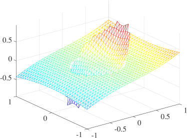
a

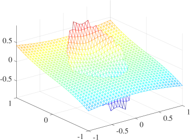
b

Figure 3: Plots of recovered gradient for Example 1. (a): $x$-component ; (b): $y$-component.

Example 5.2. In this example, we consider the flower-shape interface problem with non-homogeneous jump conditions as studied in [44, 59]. The interface curve $\Gamma$ in polar coordinates is given by

$$r=\frac{1}{2}+\frac{\sin(5\theta)}{7}.$$

It contains both convex and concave parts, as demonstrated in Figure 4a. The diffusion coefficient is piecewise constant with $\beta_{1}=1$ and $\beta_{2}=10$. The right-hand side function $f$ in (2.1a) is chosen to match the exact solution

$$u(x,y)=\left\{\begin{array}[]{ll}e^{(x^{2}+y^{2})},&\text{if }(x,y)\in\Omega_{1}\\ 0.1(x^{2}+y^{2})^{2}-0.01\ln(2\sqrt{x^{2}+y^{2}}),&\text{if }(x,y)\in\Omega_{2},\\ \end{array}\right.$$

and the jump conditions (2.1c)-(2.1d) are provided by the exact solution.

In Figure 4b, we plot the numerical solution on the initial mesh which clearly indicates the non-homogeneous jump in function value. We show the numerical results in Table 5. As expected, we observe the first-order convergence for the gradient of finite element solution. For the recovered gradient, $\mathcal{O}(h^{1.5})$ convergence is observed, which is in agreement with Theorem 4.2. The recovered gradient on the initial mesh is visualized in Figure 5.

Table 5: Numerical results for Example 5.2.

$h$	$De$	order	$D^{i}e$	order	$D^{r}_{r}e$	order
1/16	8.86e-02	–	5.81e-02	–	3.74e-02	–
1/32	3.90e-02	1.19	1.50e-02	1.95	1.19e-02	1.65
1/64	1.90e-02	1.04	4.37e-03	1.78	3.57e-03	1.74
1/128	9.48e-03	1.00	1.57e-03	1.48	1.29e-03	1.47
1/256	4.74e-03	1.00	5.63e-04	1.48	4.72e-04	1.45
1/512	2.37e-03	1.00	2.00e-04	1.50	1.71e-04	1.47
1/1024	1.18e-03	1.00	7.06e-05	1.50	6.62e-05	1.37

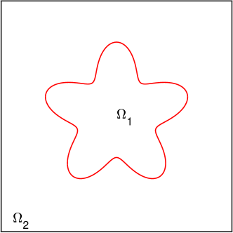
a

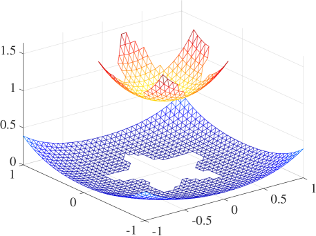
b

Figure 4: Plots for Example 4. (a): Plot of the interface; (b): Plot of numerical solution.

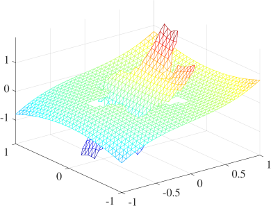
a

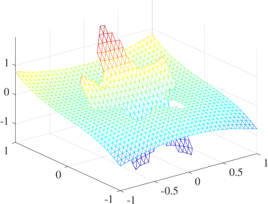
b

Figure 5: Plots of recovered gradient for Example 2 on the initial mesh. (a): $x$-component ; (b): $y$-component.

Example 5.3. In this example, we consider the interface problem with complex geometrical structure as in [45]. The interface in polar coordinates is given by

$$r=0.40178(1+\cos(2\theta)\sin(6\theta))\cos(\theta).$$

The interface and subdomains are plotted in Figure 4a. The coefficient function is

$$\beta(x,y)=\left\{\begin{array}[]{ll}(x^{2}-y^{2}-7)/7,&(x,y)\in\Omega_{1},\\ (xy+2)/5,&(x,y)\in\Omega_{2};\end{array}\right.$$

and the exact function is

$$u(x,y)=\left\{\begin{array}[]{ll}\sin(x+y)+\cos(x+y)+1,&(x,y)\in\Omega_{1},\\ x+y+1,&(x,y)\in\Omega_{2}.\end{array}\right.$$

As plotted in Figure 6a, the interface contains complex geometrical structure. To guarantee the Assumption 2.2, we need an extremely fine mesh. It would increase the computational cost. To reduce the computational cost, we propose an adaptive strategy to generate an initial unfitted mesh. Here we use the curvature-based a posterior estimator to guide the refinement of the mesh as in [53]. Different from the mesh generated in [53], the resulted mesh is an unfitted mesh and all triangles are perfect right triangles.

Figure 6b plots the generated initial unfitted mesh. It is easy to see that the mesh is refined around the part of the interface with high curvature. The other four levels of unfitted meshes are obtained by uniform refinement. The numerical results are summarized in Table 6. Note that in Table 6, convergence rates are listed with respect to the degree of freedom (DOF). The corresponding convergent rates with respect to the mesh size $h$ are double of what we present in Table 6. The gradient of finite element solution converges to the exact gradient at the rate of $\mathcal{O}(h)$ while the recovered gradient superconverges at the rate of $\mathcal{O}(h^{1.5})$. Additionally, the predicted supercloseness is observed in the numerical experiment.

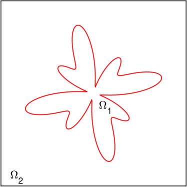
a

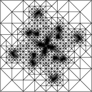
b

Figure 6: Plots for Example 3. (a): Plot of the interface; (b): Initial unfitted mesh;

Table 6: Numerical results for Example 5.3.

DOF	$De$	order	$D^{i}e$	order	$D^{r}_{r}e$	order
2573	2.49e-02	–	1.32e-02	–	8.68e-03	–
10265	1.29e-02	0.48	4.42e-03	0.79	3.20e-03	0.72
41009	6.57e-03	0.49	1.56e-03	0.75	1.25e-03	0.68
163937	3.30e-03	0.50	5.09e-04	0.81	4.46e-04	0.74
655553	1.66e-03	0.50	1.74e-04	0.77	1.59e-04	0.74
2621825	8.28e-04	0.50	5.92e-05	0.78	5.48e-05	0.77

Example 5.4. In this example, we consider the interface problem as in [6, 53]. The interface in parametric form is given by

$$\left\{\begin{array}[]{ll}x(t)=r(t)\cos(\theta(t)),\\ y(t)=r(t)\sin(\theta(t));\end{array}\right.$$

where

$$\theta(t)=t+\sin(4t),\quad r(t)=0.60125+0.24012\cos(4t+\pi/2).$$

The coefficient function is

$$\beta(x,y)=\left\{\begin{array}[]{ll}4+\sin(x+y),&(x,y)\in\Omega_{1},\\ 10+x^{2}+y^{2},&(x,y)\in\Omega_{2};\end{array}\right.$$

and the exact solution is

$$u(x,y)=\left\{\begin{array}[]{ll}\sin(x)\cos(y),&(x,y)\in\Omega_{1},\\ 1-x^{2}-y^{2},&(x,y)\in\Omega_{2}.\end{array}\right.$$

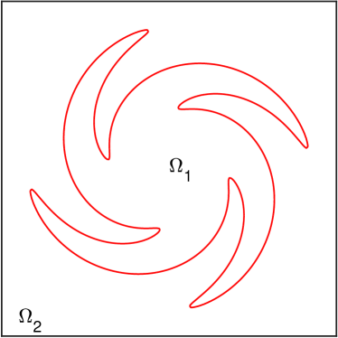
a

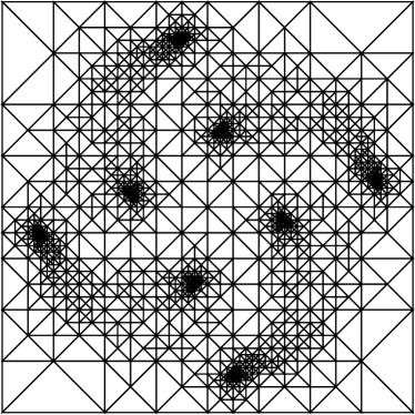
b

Figure 7: Plots for Example 4. (a): Plot of the interface; (b): Initial unfitted mesh;

Table 7: Numerical results for Example 5.4.

DOF	$De$	order	$D^{i}e$	order	$D^{r}_{r}e$	order
1381	2.14e-01	–	9.04e-02	–	8.01e-02	–
5489	1.12e-01	0.47	2.51e-02	0.93	2.02e-02	1.00
21889	5.67e-02	0.49	7.60e-03	0.86	6.65e-03	0.80
87425	2.85e-02	0.50	2.32e-03	0.86	2.11e-03	0.83
349441	1.42e-02	0.50	7.29e-04	0.83	6.99e-04	0.80
1397249	7.12e-03	0.50	2.43e-04	0.79	2.39e-04	0.78

The interface $\Gamma$, shown in Figure 7a, contains complex geometrical structure. We use the same algorithm as in Example 5.3 to generate an initial unfitted mesh which is plotted in Figure 7b. Table 7 lists the numerical results. Clearly, we observe the desired optimal convergence and superconvergence rates.

Example 5.5. In this example, we consider the interface problem as in [37, 53]. The interface $\Gamma$ in parametric form is defined by

$$\left\{\begin{array}[]{ll}x(t)=r(\theta)\cos(\theta)+x_{c},\\ y(t)=r(\theta)\sin(\theta)+y_{c};\end{array}\right.$$

where $r(\theta)=r_{0}+r_{1}\sin(\omega\theta)$, $0\leq\theta<2\pi$.

In this test, we take $r_{0}=0.4$, $r_{1}=0.2$, $\omega=20$, and $x_{c}=y_{c}=0.02\sqrt{5}$. The coefficient $\beta$ is a piecewise constant with $\beta_{1}=1$ and $\beta_{2}=10$. The exact function is

$$u(x,y)=\left\{\begin{array}[]{ll}r^{2}/\beta_{1},&(x,y)\in\Omega_{1},\\ (r^{4}-0.1\log(2r))/\beta_{2},&(x,y)\in\Omega_{2}.\end{array}\right.$$

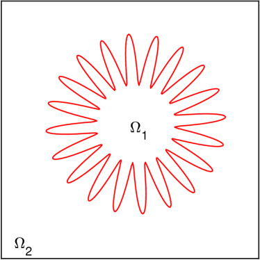
a

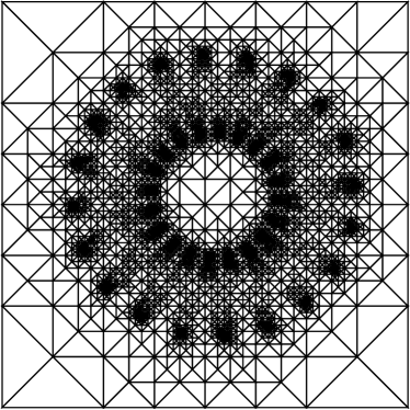
b

Figure 8: Plots for Example 5. (a): Plot of the interface; (b): Initial unfitted mesh;

Table 8: Numerical results for Example 5.5.

DOF	$De$	order	$D^{i}e$	order	$D^{r}_{r}e$	order
6514	1.30e-01	–	5.36e-02	–	4.39e-02	–
26027	6.70e-02	0.48	1.53e-02	0.91	1.58e-02	0.74
104053	3.39e-02	0.49	4.23e-03	0.93	4.74e-03	0.87
416105	1.70e-02	0.50	1.17e-03	0.93	1.32e-03	0.92
1664209	8.51e-03	0.50	3.26e-04	0.92	3.72e-04	0.91
6656417	4.25e-03	0.50	9.26e-05	0.91	9.97e-05	0.95

The interface $\Gamma$ is plotted in Figure 8a and the adaptively refined initial mesh is shown in Figure 8b. The numerical results are given in Table 8. The observed results confirm the first-order convergence rate as predicted by Theorem 2.6. For the errors $De^{i}$ and $De^{r}$, $\mathcal{O}(h^{1.8})$ order decaying rates can be observed which are better than our theoretical results. Compared to the numerical results using a body-fitted mesh in [53], we achieve the same accuracy by using an unfitted mesh with about one sixth of the total mesh grid points.

6 Conclusion

In this paper, we propose a new gradient recovery technique based on the Nitsche’s method. Compared to our previous works [20, 21, 24], it avoids the loss of accuracy of gradient near the interface caused by skinny triangles. By proving the supercloseness result for the Nitsche’s method, we are able to show that the recovered gradient is superconvergent to the exact gradient. As a byproduct, we propose a curvature estimator based adaptive algorithm to generate initial unfitted triangulations for the elliptic interface problems with complex geometry, which greatly reduces the computational cost as illustrated in Examples 5.3, 5.4 and 5.5. The future work is planned in several different directions: firstly, we will extend the study into three dimension problems; secondly, we will consider other type equations like elastic interface problems and wave propagation problems in heterogeneous media; thirdly, we will combine the curvature estimator and the recovery-based a posterior error estimator to derive adaptive algorithms for the complex interface problems.

References

- Ainsworth and Oden [2000] M. Ainsworth and J. T. Oden. A posteriori error estimation in finite element analysis. Pure and Applied Mathematics (New York). Wiley-Interscience [John Wiley & Sons], New York, 2000. ISBN 0-471-29411-X.
- Annavarapu et al. [2012] C. Annavarapu, M. Hautefeuille, and J. E. Dolbow. A robust Nitsche’s formulation for interface problems. Comput. Methods Appl. Mech. Engrg., 225/228:44–54, 2012. ISSN 0045-7825.
- Babuška [1970] I. Babuška. The finite element method for elliptic equations with discontinuous coefficients. Computing (Arch. Elektron. Rechnen), 5:207–213, 1970.
- Bank and Xu [2003] R. E. Bank and J. Xu. Asymptotically exact a posteriori error estimators. II. General unstructured grids. SIAM J. Numer. Anal., 41(6):2313–2332, 2003. ISSN 0036-1429.
- Becker et al. [2009] R. Becker, E. Burman, and P. Hansbo. A Nitsche extended finite element method for incompressible elasticity with discontinuous modulus of elasticity. Comput. Methods Appl. Mech. Engrg., 198(41-44):3352–3360, 2009. ISSN 0045-7825.
- Bedrossian et al. [2010] J. Bedrossian, J. H. von Brecht, S. Zhu, E. Sifakis, and J. M. Teran. A second order virtual node method for elliptic problems with interfaces and irregular domains. J. Comput. Phys., 229(18):6405–6426, 2010. ISSN 0021-9991.
- Belytschko and Black [1999] T. Belytschko and T. Black. A finite element method for crack growth without remeshing. Internat. J. Numer. Methods Engrg., 45(5):601–620, 1999. ISSN 0029-5981.
- Bramble and King [1996] J. H. Bramble and J. T. King. A finite element method for interface problems in domains with smooth boundaries and interfaces. Adv. Comput. Math., 6(2):109–138 (1997), 1996. ISSN 1019-7168.
- Brenner and Scott [2008] S. C. Brenner and L. R. Scott. The mathematical theory of finite element methods, volume 15 of Texts in Applied Mathematics. Springer, New York, third edition, 2008. ISBN 978-0-387-75933-3.
- Burman and Hansbo [2012] E. Burman and P. Hansbo. Fictitious domain finite element methods using cut elements: II. A stabilized Nitsche method. Appl. Numer. Math., 62(4):328–341, 2012. ISSN 0168-9274.
- Burman and Hansbo [2014] E. Burman and P. Hansbo. Fictitious domain methods using cut elements: III. A stabilized Nitsche method for Stokes’ problem. ESAIM Math. Model. Numer. Anal., 48(3):859–874, 2014. ISSN 0764-583X.
- Burman et al. [2015] E. Burman, S. Claus, P. Hansbo, M. G. Larson, and A. Massing. CutFEM: discretizing geometry and partial differential equations. Internat. J. Numer. Methods Engrg., 104(7):472–501, 2015. ISSN 0029-5981.
- Chen and Xu [2007] L. Chen and J. Xu. A posteriori error estimator by post-processing. In Jinchao Xu and Tao Tang, editors, Adaptive Computations: Theory and Algorithms, pages 34–67. Science Press, Beijing, 2007.
- Chen and Zou [1998] Z. Chen and J. Zou. Finite element methods and their convergence for elliptic and parabolic interface problems. Numer. Math., 79(2):175–202, 1998. ISSN 0029-599X.
- Chou [2012] S.-H. Chou. An immersed linear finite element method with interface flux capturing recovery. Discrete Contin. Dyn. Syst. Ser. B, 17(7):2343–2357, 2012. ISSN 1531-3492.
- Chou and Attanayake [2017] S. H. Chou and C. Attanayake. Flux recovery and superconvergence of quadratic immersed interface finite elements. Int. J. Numer. Anal. Model., 14(1):88–102, 2017. ISSN 1705-5105.
- Ciarlet [2002] P. G. Ciarlet. The finite element method for elliptic problems, volume 40 of Classics in Applied Mathematics. Society for Industrial and Applied Mathematics (SIAM), Philadelphia, PA, 2002. ISBN 0-89871-514-8. Reprint of the 1978 original [North-Holland, Amsterdam; MR0520174 (58 #25001)].
- Evans [2010] L. C. Evans. Partial differential equations, volume 19 of Graduate Studies in Mathematics. American Mathematical Society, Providence, RI, second edition, 2010. ISBN 978-0-8218-4974-3.
- Fries and Belytschko [2010] T.-P. Fries and T. Belytschko. The extended/generalized finite element method: an overview of the method and its applications. Internat. J. Numer. Methods Engrg., 84(3):253–304, 2010. ISSN 0029-5981. doi: 10.1002/nme.2914. URL http://dx.doi.org/10.1002/nme.2914.
- Guo and Yang [2016] H. Guo and X. Yang. Gradient recovery for elliptic interface problem: I. body-fitted mesh, 2016. arXiv:1607.05898 [math.NA].
- Guo and Yang [2017a] H. Guo and X. Yang. Gradient recovery for elliptic interface problem: II. immersed finite element methods. Journal of Computational Physics, 338:606 – 619, 2017a. ISSN 0021-9991.
- Guo and Yang [2017b] H. Guo and X. Yang. Polynomial preserving recovery for high frequency wave propagation. J. Sci. Comput., 71(2):594–614, 2017b. doi: 10.1007/s10915-016-0312-8.
- Guo and Zhang [2015] H. Guo and Z. Zhang. Gradient recovery for the Crouzeix-Raviart element. J. Sci. Comput., 64(2):456–476, 2015. ISSN 0885-7474.
- Guo et al. [2017] H. Guo, X. Yang, and Z. Zhang. Superconvergence analysis of partially penalized immersed finite element method, 2017. arXiv:1702.02603[math.NA].
- Hansbo and Hansbo [2002] A. Hansbo and P. Hansbo. An unfitted finite element method, based on Nitsche’s method, for elliptic interface problems. Comput. Methods Appl. Mech. Engrg., 191(47-48):5537–5552, 2002. ISSN 0045-7825.
- Hansbo and Hansbo [2004] A. Hansbo and P. Hansbo. A finite element method for the simulation of strong and weak discontinuities in solid mechanics. Comput. Methods Appl. Mech. Engrg., 193(33-35):3523–3540, 2004. ISSN 0045-7825.
- Hansbo et al. [2003] A. Hansbo, P. Hansbo, and M. G. Larson. A finite element method on composite grids based on Nitsche’s method. M2AN Math. Model. Numer. Anal., 37(3):495–514, 2003. ISSN 0764-583X.
- Hansbo [2005] P. Hansbo. Nitsche’s method for interface problems in computational mechanics. GAMM-Mitt., 28(2):183–206, 2005. ISSN 0936-7195. doi: 10.1002/gamm.201490018. URL http://dx.doi.org/10.1002/gamm.201490018.
- Hansbo et al. [2014] P. Hansbo, M. G. Larson, and S. Zahedi. A cut finite element method for a Stokes interface problem. Appl. Numer. Math., 85:90–114, 2014. ISSN 0168-9274.
- Hou and Liu [2005] S. Hou and X.-D. Liu. A numerical method for solving variable coefficient elliptic equation with interfaces. J. Comput. Phys., 202(2):411–445, 2005. ISSN 0021-9991.
- Hou et al. [2010] S. Hou, W. Wang, and L. Wang. Numerical method for solving matrix coefficient elliptic equation with sharp-edged interfaces. J. Comput. Phys., 229(19):7162–7179, 2010. ISSN 0021-9991.
- Hou et al. [2013] S. Hou, P. Song, L. Wang, and H. Zhao. A weak formulation for solving elliptic interface problems without body fitted grid. J. Comput. Phys., 249:80–95, 2013. ISSN 0021-9991.
- Hou et al. [2004] T. Y. Hou, X.-H. Wu, and Y. Zhang. Removing the cell resonance error in the multiscale finite element method via a Petrov-Galerkin formulation. Commun. Math. Sci., 2(2):185–205, 2004. ISSN 1539-6746.
- Ji et al. [2014] H. Ji, J. Chen, and Z. Li. A symmetric and consistent immersed finite element method for interface problems. J. Sci. Comput., 61(3):533–557, 2014. ISSN 0885-7474.
- LeVeque and Li [1994] R. J. LeVeque and Z. Li. The immersed interface method for elliptic equations with discontinuous coefficients and singular sources. SIAM J. Numer. Anal., 31(4):1019–1044, 1994. ISSN 0036-1429.
- Li [1998a] Z. Li. The immersed interface method using a finite element formulation. Appl. Numer. Math., 27(3):253–267, 1998a. ISSN 0168-9274.
- Li [1998b] Z. Li. A fast iterative algorithm for elliptic interface problems. SIAM J. Numer. Anal., 35(1):230–254, 1998b. ISSN 0036-1429.
- Li and Ito [2006] Z. Li and K. Ito. The immersed interface method, volume 33 of Frontiers in Applied Mathematics. Society for Industrial and Applied Mathematics (SIAM), Philadelphia, PA, 2006. ISBN 0-89871-609-8. Numerical solutions of PDEs involving interfaces and irregular domains.
- Li et al. [2003] Z. Li, T. Lin, and X. Wu. New Cartesian grid methods for interface problems using the finite element formulation. Numer. Math., 96(1):61–98, 2003. ISSN 0029-599X.
- Li et al. [2004] Z. Li, T. Lin, Y. Lin, and R. C. Rogers. An immersed finite element space and its approximation capability. Numer. Methods Partial Differential Equations, 20(3):338–367, 2004. ISSN 0749-159X.
- Li et al. [2017] Z. Li, H. Ji, and X. Chen. Accurate solution and gradient computation for elliptic interface problems with variable coefficients. SIAM J. Numer. Anal., 55(2):570–597, 2017.
- Lin et al. [2015] T. Lin, Y. Lin, and X. Zhang. Partially penalized immersed finite element methods for elliptic interface problems. SIAM J. Numer. Anal., 53(2):1121–1144, 2015. ISSN 0036-1429. doi: 10.1137/130912700. URL http://dx.doi.org/10.1137/130912700.
- Moës et al. [2001] N. Moës, J. Dolbow, and T. Belytschko. A finite element method for crack growth without remeshing. Internat. J. Numer. Methods Engrg., 51(3):293–313, 2001. ISSN 0029-5981.
- Mu et al. [2013] L. Mu, J. Wang, G. Wei, X. Ye, and S. Zhao. Weak Galerkin methods for second order elliptic interface problems. J. Comput. Phys., 250:106–125, 2013. ISSN 0021-9991.
- Mu et al. [2016] L. Mu, J. Wang, X. Ye, and S. Zhao. A new weak Galerkin finite element method for elliptic interface problems. J. Comput. Phys., 325:157–173, 2016. ISSN 0021-9991.
- Naga and Zhang [2004] A. Naga and Z. Zhang. A posteriori error estimates based on the polynomial preserving recovery. SIAM J. Numer. Anal., 42(4):1780–1800 (electronic), 2004. ISSN 0036-1429.
- Naga and Zhang [2005] A. Naga and Z. Zhang. The polynomial-preserving recovery for higher order finite element methods in 2D and 3D. Discrete Contin. Dyn. Syst. Ser. B, 5(3):769–798, 2005. ISSN 1531-3492.
- Nitsche [1971] J. Nitsche. über ein Variationsprinzip zur Lösung von Dirichlet-Problemen bei Verwendung von Teilräumen, die keinen Randbedingungen unterworfen sind. Abh. Math. Sem. Univ. Hamburg, 36:9–15, 1971. ISSN 0025-5858. Collection of articles dedicated to Lothar Collatz on his sixtieth birthday.
- Peskin [1977] C. S. Peskin. Numerical analysis of blood flow in the heart. J. Computational Phys., 25(3):220–252, 1977. ISSN 0021-9991.
- Peskin [2002] C. S. Peskin. The immersed boundary method. Acta Numer., 11:479–517, 2002. ISSN 0962-4929.
- Qin et al. [2017] F. Qin, Z. Wang, Z. Ma, and Z. Li. Accurate gradient computations at interfaces using finite element methods, 2017. arXiv:1703.00093 [math.NA].
- Wadbro et al. [2013] E. Wadbro, S. Zahedi, G. Kreiss, and M. Berggren. A uniformly well-conditioned, unfitted Nitsche method for interface problems. BIT, 53(3):791–820, 2013. ISSN 0006-3835.
- Wei et al. [2014] H. Wei, L. Chen, Y. Huang, and B. Zheng. Adaptive mesh refinement and superconvergence for two-dimensional interface problems. SIAM J. Sci. Comput., 36(4):A1478–A1499, 2014. ISSN 1064-8275.
- Xu [1982] J. Xu. Error estimates of the finite element method for the 2nd order elliptic equations with discontinuous coefficients. J. Xiangtan Univ., 1:1–5, 1982.
- Xu and Zhang [2004] J. Xu and Z. Zhang. Analysis of recovery type a posteriori error estimators for mildly structured grids. Math. Comp., 73(247):1139–1152 (electronic), 2004. ISSN 0025-5718.
- Zhang [2007] Z. Zhang. Recovery techniques in finite element methods. In Jinchao Xu and Tao Tang, editors, Adaptive Computations: Theory and Algorithms, pages 297–365. Science Press, Beijing, 2007.
- Zhang and Naga [2005] Z. Zhang and A. Naga. A new finite element gradient recovery method: superconvergence property. SIAM J. Sci. Comput., 26(4):1192–1213 (electronic), 2005. ISSN 1064-8275.
- Zheng and Lowengrub [2016] X. Zheng and J. Lowengrub. An interface-fitted adaptive mesh method for elliptic problems and its application in free interface problems with surface tension. Adv. Comput. Math., 42(5):1225–1257, 2016. ISSN 1019-7168.
- Zhou and Wei [2006] Y. C. Zhou and G. W. Wei. On the fictitious-domain and interpolation formulations of the matched interface and boundary (MIB) method. J. Comput. Phys., 219(1):228–246, 2006. ISSN 0021-9991.
- Zhou et al. [2006] Y. C. Zhou, S. Zhao, M.l Feig, and G. W. Wei. High order matched interface and boundary method for elliptic equations with discontinuous coefficients and singular sources. J. Comput. Phys., 213(1):1–30, 2006. ISSN 0021-9991.
- Zienkiewicz and Zhu [1992a] O. C. Zienkiewicz and J. Z. Zhu. The superconvergent patch recovery and a posteriori error estimates. I. The recovery technique. Internat. J. Numer. Methods Engrg., 33(7):1331–1364, 1992a. ISSN 0029-5981.
- Zienkiewicz and Zhu [1992b] O. C. Zienkiewicz and J. Z. Zhu. The superconvergent patch recovery and a posteriori error estimates. II. Error estimates and adaptivity. Internat. J. Numer. Methods Engrg., 33(7):1365–1382, 1992b. ISSN 0029-5981.
- Zienkiewicz et al. [2013] O. C. Zienkiewicz, R. L. Taylor, and J. Z. Zhu. The finite element method: its basis and fundamentals. Elsevier/Butterworth Heinemann, Amsterdam, seventh edition, 2013. ISBN 978-1-85617-633-0.