Analysis of Optimization Algorithms via Integral Quadratic Constraints: Nonstrongly Convex Problems

Abstract

In this paper, we develop a unified framework able to certify both exponential and subexponential convergence rates for a wide range of iterative first-order optimization algorithms. To this end, we construct a family of parameter-dependent nonquadratic Lyapunov functions that can generate convergence rates in addition to proving asymptotic convergence. Using Integral Quadratic Constraints (IQCs) from robust control theory, we propose a Linear Matrix Inequality (LMI) to guide the search for the parameters of the Lyapunov function in order to establish a rate bound. Based on this result, we formulate a Semidefinite Programming (SDP) whose solution yields the best convergence rate that can be certified by the class of Lyapunov functions under consideration. We illustrate the utility of our results by analyzing the gradient method, proximal algorithms and their accelerated variants for (strongly) convex problems. We also develop the continuous-time counterpart, whereby we analyze the gradient flow and the continuous-time limit of Nesterov’s accelerated method.

90C22, 90C25, 90C30, 93C10, 93D99, 93C15

1 Introduction

The analysis and design of iterative optimization algorithms is a well-established research area in optimization theory. Due to their computational efficiency and global convergence properties, first-order methods are of particular interest, especially in large-scale optimization arising in current machine learning applications. However, these algorithms can be very slow, even for moderately well-conditioned problems. In this direction, accelerated variants of first-order algorithms, such as Polyak’s Heavy-ball algorithm [25] or Nesterov’s accelerated method [22], have been developed to speed up the convergence in ill-conditioned and nonstrongly convex problems.

In numerical optimization, convergence analysis is an integral part of algorithm tuning and design. This task, however, is often pursued on a case-by-case basis and the analysis techniques heavily depend on the particular algorithm under study, as well as the underlying assumptions. However, by interpreting iterative algorithms as feedback dynamical systems, it is possible to incorporate tools from control theory to analyze and design these algorithms in a more systematic and unified manner [15, 31, 12, 30]. Moreover, control techniques can be exploited to address more complex tasks, such as analyzing robustness against uncertainties, deriving nonconservative worst-case bounds, and providing convergence guarantees under less restrictive assumptions [6, 15, 19].

A universal approach to analyzing the stability of dynamical systems is to construct a Lyapunov function that decreases along the trajectories of the system, proving asymptotic convergence. In the context of iterative optimization algorithms, it is of particular importance to certify a convergence rate in addition to proving asymptotic convergence. Construction of Lyapunov functions that can achieve this goal is not straightforward, especially for nonstrongly convex problems, in which the convergence rate is subexponential. It is important to remark that in a considerable number of applications in machine learning, the underlying optimization problem is not strongly convex [3].

The goal of the present work is to develop a semidefinite programming (SDP) framework for the construction of Lyapunov functions that can characterize both exponential and subexponential convergence rates for iterative first-order optimization algorithms. The main pillars of our framework are time-varying Lyapunov functions, originally proposed in [27] for analyzing gradient-based momentum methods [32, 33], as well as Integral Quadratic Constraints (IQCs) from robust control theory [34, 20], which have recently been adapted by Lessard et al. [19] in the context of optimization algorithms. Specifically, we propose a family of nonquadratic Lyapunov functions equipped with time-dependent parameters that can establish both exponential and subexponential convergence rates. We then develop an LMI to guide the search for the parameters of the Lyapunov function in order to generate analytical/numerical convergence rates. Based on this result, we formulate an SDP to compute the fastest convergence rate that can be certified by the class of Lyapunov functions under consideration. In this SDP, the properties of the objective function (e.g., convexity, Lipschitz continuity, etc.) can be systematically encoded into the SDP, providing a modular approach to obtaining convergence rates under various regularity assumptions, such as quasiconvexity [14], weak quasiconvexity [13], quasi-strong convexity [21], quadratic growth [21], and Polyak-$\L{}$ojasiewicz condition [17]. Furthermore, we extend our framework to continuous-time settings, in which we analyze the continuous-time limits (by taking infinitesimal stepsizes) of relevant iterative optimization algorithms. We will illustrate the generality of our framework by analyzing several first-order optimization algorithms; namely, unconstrained (accelerated) gradient methods, gradient methods with projection, and (accelerated) proximal methods.

Finally, we consider algorithm design. Specifically, we develop a robust counterpart of the developed LMI whose feasibility provides the algorithm with an additional stability margin in the sense of Lyapunov. As a design experiment, we use the LMI to tune the stepsize and momentum coefficient of Nesterov’s accelerated method applied to strongly convex functions, considering robustness as a design criterion.

1.1 Related work

There is a host of results in the literature using SDPs to analyze the convergence of first-order optimization algorithms [10, 29, 28, 18]. The first among them is [10], in which Drori and Teboulle developed an SDP to derive analytical/numerical bounds on the worst-case performance of the unconstrained gradient method and its accelerated variant. An extension of this framework to the proximal gradient method–for the case of strongly convex problems–has been recently proposed in [28]. These SDP formulations, despite being able to yield new performance bounds, are highly algorithm dependent. To depart from classical algorithmic view, Lessard et. al [19] developed an SDP framework based on quadratic Lyapunov functions and IQCs to derive sufficient conditions for exponential stability of an algorithm when the objective function is strongly convex[19, Theorem 4]. Specifically, they formulate a small SDP whose feasibility verifies exponential convergence at a specified rate. It is important to remark that Lessard’s framework is specifically tailored to analyze strongly convex problems with exponential convergence [19, 24] and subexponential rates cannot be captured. Finally, another related work is by Hu and Lessard [16], in which they have independently proposed an LMI framework based on quadratic Lyapunov functions and dissipativity theory to analyze Nesterov’s accelerated method. In contrast, the present work, inspired by [19], develops an IQC framework using time-dependent nonquadratic Lyapunov functions for the analysis of a broader family of functionals, as well as algorithms involving projections and proximal operators, including the proximal variant of Nesterov’s method.

1.2 Notation and preliminaries

We denote the set of real numbers by $\mathbb{R}$, the set of real $n$-dimensional vectors by $\mathbb{R}^{n}$, the set of $m\times n$-dimensional matrices by $\mathbb{R}^{m\times n}$, and the $n$-dimensional identity matrix by $I_{n}$. We denote by $\mathbb{S}^{n}$, $\mathbb{S}_{+}^{n}$, and $\mathbb{S}_{++}^{n}$ the sets of $n$-by-$n$ symmetric, positive semidefinite, and positive definite matrices, respectively. For $M\in\mathbb{R}^{n\times n}$ and $x\in\mathbb{R}^{n}$, we have that $x^{\top}Mx=\frac{1}{2}x^{\top}(M+M^{\top})x$. The $p$-norm ($p\geq 1$) is displayed by $\|\cdot\|_{p}\colon\mathbb{R}^{n}\to\mathbb{R}_{+}$. For two matrices $A\in\mathbb{R}^{m\times n}$ and $B\in\mathbb{R}^{p\times q}$ of arbitrary dimensions, their Kronecker product is given by

$$A\otimes B=\begin{bmatrix}A_{11}B&\cdots&A_{1n}B\\ \vdots&\ddots&\vdots\\ A_{m1}B&\ldots&A_{mn}B\end{bmatrix}.$$

Further, we have that $(A\otimes B)^{\top}=A^{\top}\otimes B^{\top}$ and $(AC)\otimes(BD)=(A\otimes B)(C\otimes D)$, for matrices of appropriate dimensions. Let $f\colon\mathbb{R}^{n}\to\mathbb{R}\cup\{+\infty\}$ be a closed proper function. The effective domain of $f$ is denoted by $\mathrm{dom}\,f=\{x\in\mathbb{R}^{n}\colon f(x)<\infty\}$. The indicator function $\mathbb{I}_{\mathcal{X}}\colon\mathbb{R}^{n}\to\mathbb{R}\cup\{+\infty\}$ of a closed nonempty convex set $\mathcal{X}\subset\mathbb{R}^{n}$ is defined as $\mathbb{I}_{\mathcal{X}}(x)=0$ if $x\in\mathcal{X}$, and $\mathbb{I}_{\mathcal{X}}(x)=+\infty$ otherwise. The Euclidean projection of $x\in\mathbb{R}^{n}$ onto a set $\mathcal{X}$ is denoted by $[x]_{\mathcal{X}}=\mathrm{argmin}_{y\in\mathcal{X}}\|y-x\|_{2}$.

Definition 1.1 (Smoothness)

A differentiable function $f\colon\mathbb{R}^{d}\to\mathbb{R}$ is $L_{f}$-smooth on $\mathcal{S}\subseteq\mathrm{dom}\,f$ if the following inequality holds.

(1.1) $$\|\nabla f(x)-\nabla f(y)\|_{2}\leq L_{f}\|x-y\|_{2}\quad\mbox{for all}\ x,y\in\mathcal{S}.$$

An equivalent definition is that

(1.2) $$f(y)\leq f(x)+\nabla f(x)^{\top}(y-x)+\dfrac{L_{f}}{2}\|y-x\|_{2}^{2}\quad\text{for all}\ x,y\in\mathcal{S}.$$

Definition 1.2 (Strong convexity)

A differentiable function $f\colon\mathbb{R}^{d}\to\mathbb{R}$ is $m_{f}$-strongly convex on $\mathcal{S}\subseteq\mathrm{dom}\,f$ if the following inequality holds.

(1.3) $$m_{f}\|x-y\|_{2}^{2}\leq(x-y)^{\top}(\nabla f(x)-\nabla f(y))\quad\text{for all}\ x,y\in\mathcal{S}.$$

An equivalent definition is that

(1.4) $$f(x)+\nabla f(x)^{\top}(y-x)+\dfrac{m_{f}}{2}\|y-x\|_{2}^{2}\leq f(y)\quad\text{for all}\ x,y\in\mathcal{S}.$$

We denote the class of $L_{f}$-smooth and $m_{f}$-strongly convex functions by $\mathcal{F}(m_{f},L_{f})$. Note that, by setting $m_{f}=0$, we recover convex functions. For the class $\mathcal{F}(m_{f},L_{f})$, we denote the condition number by $\kappa_{f}=L_{f}/m_{f}\geq 1$.

2 Algorithm representation

Iterative algorithms can be represented as linear dynamical systems interacting with one or more static nonlinearities [19]. The linear part describes the algorithm itself, while the nonlinear components depend exclusively on the first-order oracle of the objective function. In this paper, we consider first-order algorithms that have the following state-space representation,

(2.1) $$\xi_{k+1} =A_{k}\xi_{k}+B_{k}u_{k},$$

$$y_{k} =C_{k}\xi_{k},$$

$$u_{k} =\phi(y_{k}),$$

$$x_{k} =E_{k}\xi_{k},$$

where at each iteration index $k$, $\xi_{k}\in\mathbb{R}^{n}$ is the state, $u_{k}\in\mathbb{R}^{d}$ is the input ($d\leq n$), $y_{k}\in\mathbb{R}^{d}$ is the feedback output that is transformed by the nonlinear map $\phi\colon\mathbb{R}^{d}\to\mathbb{R}^{d}$ to generate $u_{k}$, and $x_{k}\in\mathbb{R}^{d}$ is the output at which the suboptimality will be evaluated for convergence analysis. See Figure 1 for a block diagram representation.

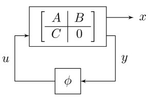
Figure 1: Block diagram representation of a first-order algorithm in state-space form.

A broad family of first-order algorithms can be represented in the canonical form (2.1), where the matrices $(A_{k},B_{k},C_{k},E_{k})$ differ for each algorithm. In this representation, the nonlinear feedback component $\phi$ depends on the oracle of the objective function. For instance, in unconstrained smooth minimization problems, we have that $\phi=\nabla f$, where $f$ is the objective function. In composite optimization problems, $\phi$ is the generalized gradient mapping of the composite function, which we will describe in $\S$5. As an illustration, consider the following recursion defined on the two sequences $\{x_{k}\}$ and $\{y_{k}\}$,

(2.2) $$x_{k+1} =x_{k}+\beta_{k}(x_{k}-x_{k-1})-h_{k}\nabla f(y_{k}),$$

$$y_{k} =x_{k}+\gamma_{k}(x_{k}-x_{k-1}),$$

where $h_{k},\beta_{k}$ and $\gamma_{k}$ are nonnegative scalars, $\{x_{k}\}$ is the primary sequence, and $\{y_{k}\}$ is the sequence at which the gradient is evaluated. By defining the state vector $\xi_{k}=[x_{k-1}^{\top}\ x_{k}^{\top}]^{\top}\in\mathbb{R}^{2d}$, we can represent (2.2) in the canonical form (2.1), where the matrices $(A_{k},B_{k},C_{k})$ are given by

(2.7) $$\left[\begin{array}[]{c|c}A_{k}&B_{k}\\ \hline\cr C_{k}&0\end{array}\right]=\left[\begin{array}[]{c|c}\begin{matrix}0&I_{d}\\ -\beta_{k}I_{d}&(\beta_{k}+1)I_{d}\end{matrix}&\begin{matrix}0\\ -h_{k}I_{d}\end{matrix}\\ \hline\cr\begin{matrix}-\gamma_{k}I_{d}&(\gamma_{k}+1)I_{d}\end{matrix}&0\end{array}\right].$$

Notice that depending on the selection of $\beta_{k}$ and $\gamma_{k}$, (2.2) describes various existing algorithms. For example, the gradient method corresponds to the case $\beta_{k}=\gamma_{k}=0$. In Nesterov’s accelerated method, we have $\beta_{k}=\gamma_{k}$. Finally, we recover the Heavy-ball method by setting $\gamma_{k}=0$.

For an algorithm represented in the canonical form (2.1), its fixed points (if they exist) are characterized by

(2.8) $$\xi_{\star}=A_{k}\xi_{\star}+B_{k}u_{\star},\ \ y_{\star}=C_{k}\xi_{\star},\ \ u_{\star}=\phi(y_{\star}),\ \ x_{\star}=E_{k}\xi_{\star}\ \ \mbox{for all }k.$$

For well-designed algorithms, the fixed-point equation must coincide with the optimality conditions of the underlying optimization problem.

3 Main results

In this paper, we are concerned with the convergence analysis of first-order algorithms designed to solve optimization problems of the form

(3.1) $$\mathcal{X}_{\star}=\mathrm{argmin}_{x\in\mathbb{R}^{d}}\{F(x)=f(x)+g(x)\},$$

where $f\colon\mathbb{R}^{d}\to\mathbb{R}$ is closed, proper, and differentiable, while $g\colon\mathbb{R}^{d}\to\mathbb{R}\cup\{+\infty\}$ is closed convex proper (CCP), and possibly nondifferentiable. Depending on the choice of $f$ and $g$, (3.1) describes various specialized optimization problems. For instance, when $g(x)=\mathbb{I}_{\mathcal{X}}(x)$ is the indicator function of a nonempty, closed, convex set $\mathcal{X}\subseteq\mathbb{R}^{d}$, (3.1) is equivalent to constrained smooth programming; when $g(x)\equiv 0$, we obtain unconstrained smooth programming; and, when $f(x)\equiv 0$, (3.1) simplifies to an unconstrained nonsmooth optimization problem. In all cases, we assume that the optimal solution set $\mathcal{X}_{\star}$ is nonempty and closed, and the optimal value $F_{\star}=\inf_{x\in\mathbb{R}^{d}}\ F(x)$ is finite.

Consider an iterative first-order algorithm, represented in the state-space form (2.1), that under appropriate initialization solves (3.1) asymptotically; that is, the sequence of outputs $\{x_{k}\}$ satisfies $\lim_{k\to\infty}F(x_{k})=F(x_{\star})$, where $x_{\star}\in\mathcal{X}_{\star}$. We assume that the fixed point $y_{\star}$ of the sequence $\{y_{k}\}$, defined in (2.8), satisfies $y_{\star}=x_{\star}$. In other words, both $\{x_{k}\}$ and $\{y_{k}\}$ are convergent to the same optimal point $x_{\star}$. To establish a rate bound for the algorithm under study, we propose the following Lyapunov function:

(3.2) $$V_{k}(x,\xi)=a_{k}(F(x)-F(x_{\star}))+(\xi-\xi_{\star})^{\top}P_{k}(\xi-\xi_{\star}),$$

where $a_{k}\geq 0,\ P_{k}\in\mathbb{S}_{+}^{n}\ \mbox{for all}\ k$, and are to be determined. The first term is the suboptimality of $x$ scaled by $a_{k}$ and the second term quantifies the suboptimality of the state $\xi$ with respect to the optimal state $\xi_{\star}$. Notice that by this definition, we have that $V_{k}(x,\xi)\geq 0$ for all $k$, and $V_{k}(x_{\star},\xi_{\star})=0$, i.e., the Lyapunov function is nonnegative everywhere and zero at optimality. Suppose we select $\{a_{k}\}$ and $\{P_{k}\}$ such that the Lyapunov function becomes nonincreasing along the trajectories of (2.1), i.e., the following condition holds.

(3.3) $$V_{k+1}(x_{k+1},\xi_{k+1})\leq V_{k}(x_{k},\xi_{k})\quad\text{for all}\ k.$$

Then, we can conclude $a_{k}(F(x_{k})-F(x_{\star}))\leq V_{k}(x_{k},\xi_{k})\leq V_{0}(x_{0},\xi_{0})$, or equivalently,

(3.4) $$0\leq F(x_{k})-F(x_{\star})\leq\dfrac{V_{0}(x_{0},\xi_{0})}{a_{k}}=\mathcal{O}(\frac{1}{a_{k}})\quad\text{for all}\ k.$$

In other words, the sequence $\{a_{k}\}$ generates an upper bound on the suboptimality or, equivalently, a lower bound on the convergence rate. As a result, the task of certifying a convergence rate for the algorithm translates into finding sufficient conditions to guarantee (3.3). In the following theorem, we develop an LMI whose feasibility is sufficient for (3.3) to hold.

Theorem 3.1 (Main result)

Let $x_{\star}\in\mathrm{argmin}_{x\in\mathbb{R}^{d}}\ F(x)$ be a minimizer of $F\colon\mathbb{R}^{d}\to\mathbb{R}\cup\{+\infty\}$ with a finite optimal value $F(x_{\star})$. Consider an iterative first-order algorithm in the state-space form (2.1).

1. Suppose the fixed points $(\xi_{\star},u_{\star},y_{\star},x_{\star})$ of (2.1) satisfy

   (3.5) $$\xi_{\star}=A_{k}\xi_{\star}+B_{k}u_{\star},\ \ y_{\star}=C_{k}\xi_{\star},\ \ u_{\star}=\phi(y_{\star}),\ \ x_{\star}=E_{k}\xi_{\star}=y_{\star}\ \ \mbox{for all }k.$$

2. Suppose there exist symmetric matrices $M_{k}^{1},M_{k}^{2},M_{k}^{3}$ such that the following inequalities hold for all $k$.

   (3.6a) $$F(x_{k+1})-F(x_{k}) \leq e_{k}^{\top}M_{k}^{1}e_{k},$$

   (3.6b) $$F(x_{k+1})-F(x_{\star}) \leq e_{k}^{\top}M_{k}^{2}e_{k},$$

   (3.6c) $$0 \leq e_{k}^{\top}M_{k}^{3}e_{k},$$

   where $e_{k}=[(\xi_{k}-\xi_{\star})^{\top}\ (u_{k}-u_{\star})^{\top}]^{\top}\in\mathbb{R}^{n+d}$ and $M_{k}^{3}$ is either zero or indefinite.

3. Suppose there exists a nonnegative and nondecreasing sequence of reals $\{a_{k}\}$, a sequence of nonnegative reals $\{\sigma_{k}\}$, and a sequence of $n\times n$ positive semidefinite matrices $\{P_{k}\}$ satisfying

   (3.7) $$M_{k}^{0}+a_{k}M_{k}^{1}+(a_{k+1}-a_{k})M_{k}^{2}+\sigma_{k}M_{k}^{3}\preceq 0\quad\mbox{for all }k,$$

   where

   (3.8) $$M_{k}^{0} =\begin{bmatrix}A_{k}^{\top}P_{k+1}A_{k}-P_{k}&A_{k}^{\top}P_{k+1}B_{k}\\ B_{k}^{\top}P_{k+1}A_{k}&B_{k}^{\top}P_{k+1}B_{k}\end{bmatrix}.$$

   Then the sequence $\{x_{k}\}$ satisfies

   (3.9) $$F(x_{k})-F(x_{\star})\leq\dfrac{a_{0}(F(x_{0})-F(x_{\star}))+(\xi_{0}-\xi_{\star})^{\top}P_{0}(\xi_{0}-\xi_{\star})}{a_{k}}\quad\mbox{for all}\ k.$$

Before proving Theorem 3.1, we briefly discuss the assumptions made in the statement of the theorem. The first inequality in (3.6) bounds the difference between two consecutive iterates. In particular, if $M_{k}^{1}$ is negative semidefinite for all $k$, then the sequence $\{F(x_{k})\}$ is monotone. The second inequality in (3.6) bounds the suboptimality; and finally, the third inequality in (3.6) is a quadratic constraint on the input-output pairs $(\xi_{k},u_{k})$ that are related via the rule $u_{k}=\phi(C_{k}\xi_{k})$. These bounds will be required to satisfy condition (3.3) and will feature heavily throughout the paper. Note that the matrices $(M_{k}^{1},M_{k}^{2},M_{k}^{3})$ in (3.6) depend on the algorithm parameters, i.e., the matrices $(A_{k},B_{k},C_{k},E_{k})$ that define the algorithm, as well as the assumptions about the objective function $F$.

Proof 3.2 (Proof of Theorem 3.1)

First, by (2.1) and (3.5), we can write

$$\xi_{k+1}-\xi_{\star} =A_{k}(\xi_{k}-\xi_{\star})+B_{k}(u_{k}-u_{\star}),$$

Using the above identity, we can write

(3.10a) $$(\xi_{k+1}-\xi_{\star})^{\top}P_{k+1}(\xi_{k+1}-\xi_{\star})\!-\!(\xi_{k}-\xi_{\star})^{\top}P_{k}(\xi_{k}-\xi_{\star})=e_{k}^{\top}M_{k}^{0}e_{k}.$$

Multiply (3.6a) by $$a_{k} (a_{k+1}-a_{k})$$ and (3.6b) by and add both sides of the resulting inequalities to obtain

(3.10b) $$a_{k+1}(F(x_{k+1})-F(x_{\star}))-a_{k}(F(x_{k})-F(x_{\star}))\leq 0.$$

By adding both sides of the inequalities in (3.10) and recalling the definition of $V_{k}(x_{k},\xi_{k})$ in (3.2), we can write

(3.11) $$V_{k+1}(x_{k+1},\xi_{k+1})\!-\!V_{k}(x_{k},\xi_{k})\leq \,e_{k}^{\top}\left(M_{k}^{0}+a_{k}M_{k}^{1}+(a_{k+1}-a_{k})M_{k}^{2}\right)e_{k}.$$

Suppose the matrix inequality in (3.7) holds. By multiplying this inequality from the left and right by $e_{k}^{\top}$ and $e_{k}$, respectively, we obtain

(3.12) $$e_{k}^{\top}\left(M_{k}^{0}+a_{k}M_{k}^{1}+(a_{k+1}-a_{k})M_{k}^{2}+\sigma_{k}M_{k}^{3}\right)e_{k}\leq 0.$$

Finally, adding both sides of (3.11) and (3.12) yields

(3.13) $$V_{k+1}(x_{k+1},\xi_{k+1})-V_{k}(x_{k},\xi_{k})\leq-\sigma_{k}e_{k}^{\top}M_{k}^{3}e_{k}\leq 0,$$

where the second inequality follows from (3.6c). Hence, the sequence $\{V_{k}(x_{k},\xi_{k})\}$ is nonincreasing, implying $a_{k}(F(x_{k})-F(x_{\star}))\leq V_{k}(x_{k},\xi_{k})\leq V_{0}(x_{0},\xi_{0})$. The proof becomes complete by dividing both sides of the last inequality by $a_{k}$.

Some remarks are in order regarding Theorem 3.1:

1. We do not make the assumption that the algorithm under consideration is a descent method. In other words, the sequence $\{F(x_{k})\}$ of function values is not necessarily monotone, which is a hallmark of accelerated algorithms [23]. In contrast, we require the sequence $\{V_{k}(x_{k},\xi_{k})\}$ of “energy” values to be monotonically decreasing. From this perspective, the LMI (3.7) provides a guideline for the construction energy functions with this property.

2. There is no restriction on the sequence $\{a_{k}\}$ other than nonnegativity and monotonicity. Hence, we can characterize both exponential ($a_{k}=\rho^{-k},0\leq\rho<1$) and subexponential ($a_{k}=k^{p},\ p>0$, for example) convergence rates.

3. We have made no explicit assumptions about the objective function in Theorem 3.1, other than the quadratic bounds in (3.6). In fact, the matrices $M_{k}^{1},M_{k}^{2},M_{k}^{3}$ that characterize these bounds depend on the parameters of the algorithm (e.g. stepsize, momentum coefficient, etc.), as well as the assumptions about $F$. In $\S$4 and $\S$5, we will describe a general procedure for deriving these matrices for a wide range of algorithms and assumptions.

3.1 Time-invariant algorithms with exponential convergence

In this subsection, we specialize the results of Theorem 3.1 to time-invariant algorithms with exponential convergence. Under these assumptions, we can precondition $a_{k}$ and $P_{k}$ to simplify the LMI in (3.7). Explicitly, suppose the matrices $(A_{k},B_{k},C_{k},E_{k})$ that define the algorithm do not change with $k$. By the particular selection

(3.14) $$a_{k}=\rho^{-2k}a_{0},\quad a_{0}>0,\quad P_{k}=\rho^{-2k}P_{0},\quad P_{0}\succeq 0,\quad 0<\rho\leq 1\quad\mbox{for all }k,$$

the Lyapunov function in (3.2) reads as

(3.15) $$V_{k}(\xi)=\rho^{-2k}\left(a_{0}(F(x)\!-\!F(x_{\star}))+(\xi-\xi_{\star})^{\top}P_{0}(\xi-\xi_{\star})\right).$$

The unknown parameters of the Lyapunov function are now $a_{0}>0,P_{0}\succeq 0$, and the decay rate $0<\rho\leq 1$. With this parameter selection, the LMI in (3.7) simplifies greatly. The following result is a special case of Theorem 3.1 for the selection (3.14).

Theorem 3.3 (Exponential convergence of time-invariant algorithms)

In theorem 3.1, assume that the algorithm parameters as well as the matrices $M_{k}^{1},M_{k}^{2},M_{k}^{3}$ in (3.6) do not change with $k$. In other words,

$$(A_{k},B_{k},C_{k},E_{k},M_{k}^{1},M_{k}^{2},M_{k}^{3})=(A_{0},B_{0},C_{0},E_{0},M_{0}^{1},M_{0}^{2},M_{0}^{3})\quad\mbox{for all }k.$$

Suppose there exists $a_{0}>0$, $P_{0}\in\mathbb{S}_{+}^{n}$, and $\lambda_{0}\geq 0$ that satisfy

(3.16) $$\begin{bmatrix}A_{0}^{\top}P_{0}A_{0}-\rho^{2}P_{0}&A_{0}^{\top}P_{0}B_{0}\\ B_{0}^{\top}P_{0}A_{0}&B_{0}^{\top}P_{0}B_{0}\end{bmatrix}+a_{0}\rho^{2}M_{0}^{1}+a_{0}(1\!-\!\rho^{2})M_{0}^{2}+\lambda_{0}M_{0}^{3}\preceq 0,$$

for some $0<\rho\leq 1$. Then the sequence $\{x_{k}\}$ satisfy

(3.17) $$F(x_{k})-F(x_{\star})\leq\frac{a_{0}(F(x_{0})\!-\!F(x_{\star}))+(\xi_{0}-\xi_{\star})^{\top}P_{0}(\xi_{0}-\xi_{\star})}{a_{0}}\rho^{2k}.$$

Proof 3.4

By substituting the parameter selection (3.14) in (3.7) and factoring out the positive term $\rho^{-2k-2}$ from the resulting LMI, we obtain (3.16), which no longer depends on $k$. Utilizing Theorem 3.1, the feasibility of (3.16) ensures (3.3), which in turn implies (3.17). The proof is complete.

Remark 3.5

Regarding the parameter selection in (3.14), if we instead select $a_{k}\equiv 0$, $P_{k}=\rho^{-2k}P_{0}$ with $P_{0}\succ 0$ and $0<\rho\leq 1$, the Lyapunov function (3.2) simplifies to the quadratic function

(3.18) $$V_{k}(\xi)=\rho^{-2k}(\xi-\xi_{\star})^{\top}P_{0}(\xi-\xi_{\star}),\quad P_{0}\succ 0.$$

Correspondingly, the LMI (3.16) in Theorem 3.3 reduces to

(3.19) $$\begin{bmatrix}A_{0}^{\top}P_{0}A_{0}-\rho^{2}P_{0}&A_{0}^{\top}P_{0}B_{0}\\ B_{0}^{\top}P_{0}A_{0}&B_{0}^{\top}P_{0}B_{0}\end{bmatrix}+\lambda_{0}M_{0}^{3}\preceq 0.$$

By Theorem 3.1, if (3.19) is feasible for some $P_{0}\succ 0,\lambda_{0}\geq 0$ and $0<\rho\leq 1$, then the Lyapunov function in (3.18) would satisfy the decreasing property $V_{k+1}(\xi_{k+1})\leq V_{k}(\xi_{k})$, which translates to

$$(\xi_{k+1}-\xi_{\star})^{\top}P_{0}(\xi_{k+1}-\xi_{\star})\leq\rho^{2}(\xi_{k}-\xi_{\star})^{\top}P_{0}(\xi_{k}-\xi_{\star}),$$

or equivalently,

(3.20) $$\|\xi_{k}-\xi_{\star}\|_{2}^{2}\leq\rho^{2k}\text{cond}(P_{0})\|\xi_{0}-\xi_{\star}\|_{2}^{2}.$$

The matrix inequality (3.19) is precisely the condition derived in [19, Theorem 4] for the case of strongly convex objective functions, time-invariant first-order algorithms, and pointwise IQCs.

Having established the main result, it now remains to determine the matrices $M_{k}^{i},\ i\in\{0,1,2,3\}$ that construct the LMI in (3.7). To this end, we first need to introduce IQCs in the context of optimization algorithms.

3.2 IQCs for optimization algorithms

In control theory, there are various approaches and criteria for stability of linear dynamical systems in feedback interconnection with a memoryless and possibly time-varying nonlinearity. In this context, IQCs, originally proposed by Megretski and Rantzer [20], is a powerful tool for describing various classes of nonlinearities, and are particularly useful for LMI-based stability analysis. Lessard et al. [19] have recently adapted the theory of IQCs for use in optimization algorithms. Specifically, they translate the first-order defining properties of convex functions into various forms of IQCs for their gradient mappings. In the following, we briefly describe the notion of pointwise IQCs [19] (or quadratic constraints), that will be essential for subsequent developments.

3.2.1 Pointwise IQCs

Consider a mapping $\phi\colon\!\mathbb{R}^{d}\to\mathbb{R}^{d}$ and a chosen “reference” input-output pair $(x_{\star},\phi(x_{\star}))$, $x_{\star}\in\mathrm{dom}\,\phi$. We say that $\phi$ satisfies the pointwise IQC defined by $(Q_{\phi},x_{\star},\phi(x_{\star}))$ on $\mathcal{S}\subseteq\mathrm{dom}\,\phi$ if for all $x\in\mathcal{S}$, the following inequality holds [19].

(3.21) $$\begin{bmatrix}x-x_{\star}\\ \phi(x)-\phi(x_{\star})\end{bmatrix}^{\top}Q_{\phi}\,\begin{bmatrix}x-x_{\star}\\ \phi(x)-\phi(x_{\star})\end{bmatrix}\geq 0,$$

where $Q_{\phi}\in\mathbb{S}^{2d}$ is a symmetric, indefinite matrix. Many inequalities in optimization can be represented as IQCs of the form (3.21). For instance, suppose $\phi(x)$ is $L_{\phi}$-Lipschitz continuous on $\mathcal{S}\subseteq\mathrm{dom}\,\phi$ for some positive and finite $L_{\phi}$, i.e., $\|\phi(x)-\phi(x_{\star})\|_{2}\leq L_{\phi}\|x-x_{\star}\|_{2}$ for all $(x,x_{\star})\in\mathcal{S}\times\mathcal{S}$. By squaring both sides and rearranging terms, we obtain

(3.22) $$\begin{bmatrix}x-x_{\star}\\ \phi(x)-\phi(x_{\star})\end{bmatrix}^{\top}\begin{bmatrix}L_{\phi}^{2}I_{d}&0\\ 0&-I_{d}\end{bmatrix}\,\begin{bmatrix}x-x_{\star}\\ \phi(x)-\phi(x_{\star})\end{bmatrix}\geq 0,$$

which equivalently describes Lipschitz continuity. As another example, assume $\phi$ is a firmly nonexpansive mapping on $\mathcal{S}$. That is, for all $(x,x_{\star})\in\mathcal{S}\times\mathcal{S}$, we have that $\|\phi(x)-\phi(x_{\star})\|_{2}^{2}\leq(x-x_{\star})^{\top}(\phi(x)-\phi(x_{\star}))$. This inequality can be rewritten as

(3.23) $$\begin{bmatrix}x-x_{\star}\\ \phi(x)-\phi(x_{\star})\end{bmatrix}^{\top}\begin{bmatrix}0&\frac{1}{2}I_{d}\\ \frac{1}{2}I_{d}&-I_{d}\end{bmatrix}\,\begin{bmatrix}x-x_{\star}\\ \phi(x)-\phi(x_{\star})\end{bmatrix}\geq 0.$$

Note that by the Cauchy-Schwartz inequality, firm non-expansiveness implies Lipschitz continuity with Lipschitz parameter equal to one, i.e., (3.23) implies (3.22) with $L_{\phi}=1$. There are many other interesting properties such as monotonicity (also known as incremental passivity), one-sided Lipschitz continuity, cocoercivity, etc., that could be represented by quadratic constraints. In the next subsection, we will focus on the gradient mapping of a convex function from an IQC perspective.

3.2.2 IQCs for (strongly) convex functions

Consider the gradient mapping $\phi=\nabla f$, where $f\in\mathcal{F}(m_{f},L_{f})$. It directly follows from the definition of (strong) convexity in (1.3) that, $\nabla f$ satisfies the quadratic constraint

(3.24) $$\begin{bmatrix}x\!-\!y\\ \nabla f(x)\!-\!\nabla f(y)\end{bmatrix}^{\top}\begin{bmatrix}-m_{f}I_{d}&\frac{1}{2}I_{d}\\ \frac{1}{2}I_{d}&0\end{bmatrix}\begin{bmatrix}x\!-\!y\\ \nabla f(x)\!-\!\nabla f(y)\end{bmatrix}\geq 0.$$

Similarly, the Lipschitz inequality in (1.1) can be represented as

(3.25) $$\begin{bmatrix}x\!-\!y\\ \nabla f(x)\!-\!\nabla f(y)\end{bmatrix}^{\top}\begin{bmatrix}L_{f}^{2}I_{d}&0\\ 0&-1\end{bmatrix}\begin{bmatrix}x\!-\!y\\ \nabla f(x)\!-\!\nabla f(y)\end{bmatrix}\geq 0.$$

To combine strong convexity and Lipschitz continuity in a single inequality, we note that $\nabla f$ also satisfies [23]

(3.26) $$\frac{m_{f}L_{f}}{m_{f}\!+\!L_{f}}\|y\!-\!x\|_{2}^{2}\!+\!\frac{1}{m_{f}\!+\!L_{f}}\|\nabla f(y)\!-\!\nabla f(x)\|_{2}^{2}\leq(\nabla f(y)\!-\!\nabla f(x))^{\top}(y\!-\!x).$$

The above inequality can be represented by the following quadratic constraint [19],

(3.27) $$\begin{bmatrix}x\!-\!y\\ \nabla f(x)\!-\!\nabla f(y)\end{bmatrix}^{\top}\!Q_{f}\!\begin{bmatrix}x\!-\!y\\ \nabla f(x)\!-\!\nabla f(y)\end{bmatrix}\geq 0,\ \ Q_{f}\!=\!\begin{bmatrix}\frac{-m_{f}L_{f}}{m_{f}+L_{f}}I_{d}&\frac{1}{2}I_{d}\\ \frac{1}{2}I_{d}&\frac{-1}{m_{f}+L_{f}}I_{d}\end{bmatrix}.$$

In the language of IQCs, we can say that the map $\phi=\nabla f$ satisfies the pointwise IQC defined by $(Q_{f},x_{\star},\nabla f(x_{\star}))$, where the reference point $x_{\star}=y\in\mathcal{S}$ is arbitrary. Note that (3.27) encapsulates both (strong) convexity and Lipschitz continuity in a single IQC. It turns out that this quadratic constraint is both necessary and sufficient for the inclusion $f\in\mathcal{F}(m_{f},L_{f})$.

Non-differentiable convex functions. The above analysis can be extended to non-differentiable convex functions. Formally, the subdifferential $\partial f$ of a convex function $f\colon\mathbb{R}^{d}\to\mathbb{R}\cup\{+\infty\}$ is defined as

(3.28) $$\partial f(x)=\{\gamma\colon\gamma^{\top}(y-x)+f(x)\leq f(y),\ \forall y\in\mathrm{dom}\,f\},$$

where $\gamma$ is any subgradient of $f$, which we denote by $T_{f}(x)$. Adding the inequality in (3.28) to the same inequality but with $x$ and $y$ interchanged, we obtain

$$(T_{f}(x)-T_{f}(y))^{\top}(x-y)\geq 0,$$

which is equivalent to monotonicity of the subdifferential operator. Therefore, any subgradient of $f$ satisfies (3.27) with $L_{f}=\infty$. Note that this property holds even when $f$ is not convex.

4 Performance results for unconstrained smooth programming

In this section, we consider first-order algorithms designed to solve problems of the form

(4.1) $$x_{\star}\in\mathrm{argmin}_{x\in\mathbb{R}^{d}}\ f(x)\quad\mbox{where}\quad f\in\mathcal{F}(m_{f},L_{f}).$$

The well-known optimality condition in this case is

$$\mathcal{X}_{\star}=\{x_{\star}\in\mathrm{dom}\,f\colon\nabla f(x_{\star})=0\}.$$

We now consider an iterative first-order algorithm in the canonical form (2.1) for solving (4.1), where the feedback nonlinearity is given by $\phi=\nabla f$. Since the sequences $\{x_{k}\}$ and $\{y_{k}\}$ converge to the same fixed point in the optimal set by assumption, we must have that $\nabla f(y_{\star})=\nabla f(x_{\star})=0$. In other words, the fixed points of (2.1) satisfy

(4.2) $$\xi_{\star}=A_{k}\xi_{\star},\quad y_{\star}=C_{k}\xi_{\star},\quad u_{\star}=\nabla f(y_{\star})=0,\quad x_{\star} =E_{k}\xi_{\star}=y_{\star},\quad\mbox{for all }k.$$

In the following result, we characterize the quadratic bounds in (3.6) for the class $\mathcal{F}(m_{f},L_{f})$.

Lemma 4.1

Let $x_{\star}\in\mathrm{argmin}_{x\in\mathbb{R}^{d}}\ f(x)$ be a minimizer of $f\in\mathcal{F}(m_{f},L_{f})$ with a finite optimal value $f(x_{\star})$. Consider an iterative first-order algorithm in the state-space form (2.1) with $\phi=\nabla f$, where the fixed points $(\xi_{\star},u_{\star},y_{\star},x_{\star})$ satisfy

(4.3) $$\xi_{\star}=A_{k}\xi_{\star},\ \ y_{\star}=C_{k}\xi_{\star},\ \ u_{\star}=\nabla f(y_{\star})=0,\ \ x_{\star}=E_{k}\xi_{\star}=y_{\star}\quad\mbox{for all }k.$$

Define $e_{k}=[(\xi_{k}-\xi_{\star})^{\top}\ (u_{k}-u_{\star})^{\top}]^{\top}$. Then the following inequalities hold for all $k$.

(4.4a) $$f(x_{k+1})-f(x_{k}) \leq e_{k}^{\top}M_{k}^{1}e_{k},$$

(4.4b) $$f(x_{k+1})-f(x_{\star}) \leq e_{k}^{\top}M_{k}^{2}e_{k},$$

(4.4c) $$0 \leq e_{k}^{\top}M_{k}^{3}e_{k},$$

where $M_{k}^{1},M_{k}^{2},M_{k}^{3}$ are given by

(4.5) $$M_{k}^{1}=N_{k}^{1}+N_{k}^{2},\quad M_{k}^{2}=N_{k}^{1}+N_{k}^{3},\quad M_{k}^{3}=N_{k}^{4}.$$

with

$$N_{k}^{1}\! =\begin{bmatrix}E_{k+1}A_{k}\!-\!C_{k}&E_{k+1}B_{k}\\ 0&I_{d}\end{bmatrix}^{\top}\begin{bmatrix}\frac{L_{f}}{2}I_{d}&\frac{1}{2}I_{d}\\ \frac{1}{2}I_{d}&0\end{bmatrix}\begin{bmatrix}E_{k+1}A_{k}\!-\!C_{k}&E_{k+1}B_{k}\\ 0&I_{d}\end{bmatrix},$$

$$N_{k}^{2} =\begin{bmatrix}C_{k}-E_{k}&0\\ 0&I_{d}\end{bmatrix}^{\top}\begin{bmatrix}-\frac{m_{f}}{2}I_{d}&\frac{1}{2}I_{d}\\ \frac{1}{2}I_{d}&0\end{bmatrix}\begin{bmatrix}C_{k}-E_{k}&0\\ 0&I_{d}\end{bmatrix},$$

$$N_{k}^{3} =\begin{bmatrix}C_{k}&0\\ 0&I_{d}\end{bmatrix}^{\top}\begin{bmatrix}-\frac{m_{f}}{2}I_{d}&\frac{1}{2}I_{d}\\ \frac{1}{2}I_{d}&0\end{bmatrix}\begin{bmatrix}C_{k}&0\\ 0&I_{d}\end{bmatrix},$$

$$N_{k}^{4} =\begin{bmatrix}C_{k}&0\\ 0&I_{d}\end{bmatrix}^{\top}\begin{bmatrix}\frac{-m_{f}L_{f}}{m_{f}+L_{f}}I_{d}&\frac{1}{2}I_{d}\\ \frac{1}{2}I_{d}&\frac{-1}{m_{f}+L_{f}}I_{d}\end{bmatrix}\begin{bmatrix}C_{k}&0\\ 0&I_{d}\end{bmatrix}.$$

Proof 4.2

First, by Lipschitz continuity of $\nabla f$, we can write

(4.6) $$f(x_{k+1})-f(y_{k}) \leq\begin{bmatrix}x_{k+1}-y_{k}\\ \nabla f(y_{k})\end{bmatrix}^{\top}\begin{bmatrix}\frac{L_{f}}{2}I_{d}&\frac{1}{2}I_{d}\\ \frac{1}{2}I_{d}&0\end{bmatrix}\begin{bmatrix}x_{k+1}-y_{k}\\ \nabla f(y_{k})\end{bmatrix}.$$

From the recursion in (2.1), we have that

(4.7) $$\begin{bmatrix}x_{k+1}-y_{k}\\ \nabla f(y_{k})\end{bmatrix}=\begin{bmatrix}E_{k+1}A_{k}-C_{k}&E_{k+1}B_{k}\\ 0&I_{d}\end{bmatrix}\begin{bmatrix}\xi_{k}-\xi_{\star}\\ u_{k}-u_{\star}\end{bmatrix}.$$

Substituting (4.7) in (4.6) yields

(4.8) $$f(x_{k+1})-f(y_{k}) \leq e_{k}^{\top}N_{k}^{1}e_{k}.$$

Next, we use (strong) convexity and the identity $y_{k}-x_{k}=(C_{k}-E_{k})(\xi_{k}-\xi_{\star})$ to write

(4.9) $$f(y_{k})-f(x_{k}) \leq\begin{bmatrix}y_{k}-x_{k}\\ \nabla f(y_{k})\end{bmatrix}^{\top}\begin{bmatrix}-\frac{m_{f}}{2}I_{d}&\frac{1}{2}I_{d}\\ \frac{1}{2}I_{d}&0\end{bmatrix}\begin{bmatrix}y_{k}-x_{k}\\ \nabla f(y_{k})\end{bmatrix}$$

$$\leq e_{k}^{\top}\begin{bmatrix}C_{k}-E_{k}&0\\ 0&I_{d}\end{bmatrix}^{\top}\begin{bmatrix}-\frac{m_{f}}{2}I_{d}&\frac{1}{2}I_{d}\\ \frac{1}{2}I_{d}&0\end{bmatrix}\begin{bmatrix}C_{k}-E_{k}&0\\ 0&I_{d}\end{bmatrix}e_{k}$$

$$=e_{k}^{\top}N_{k}^{2}e_{k}.$$

Adding both sides of (4.8) and (4.9) yields

$$f(x_{k+1})-f(x_{k})\leq e_{k}^{\top}(N_{k}^{1}+N_{k}^{2})e_{k}=e_{k}^{\top}M_{k}^{1}e_{k}.$$

By (strong) convexity and the identity $y_{k}-y_{\star}=C_{k}(\xi_{k}-\xi_{\star})$, we can write

(4.10) $$f(y_{k})-f(y_{\star}) \leq\begin{bmatrix}y_{k}-y_{\star}\\ \nabla f(y_{k})\end{bmatrix}^{\top}\begin{bmatrix}-\frac{m_{f}}{2}I_{d}&\frac{1}{2}I_{d}\\ \frac{1}{2}I_{d}&0\end{bmatrix}\,\begin{bmatrix}y_{k}-y_{\star}\\ \nabla f(y_{k})\end{bmatrix}$$

$$=e_{k}^{\top}\begin{bmatrix}C_{k}&0\\ 0&I_{d}\end{bmatrix}^{\top}\begin{bmatrix}-\frac{m_{f}}{2}I_{d}&\frac{1}{2}I_{d}\\ \frac{1}{2}I_{d}&0\end{bmatrix}\begin{bmatrix}C_{k}&0\\ 0&I_{d}\end{bmatrix}e_{k}$$

$$=e_{k}^{\top}{N_{k}^{3}}e_{k}.$$

By adding both sides of (4.8) and (4.10) we obtain

$$f(x_{k+1})-f(x_{\star})\leq e_{k}^{\top}(N_{k}^{1}+N_{k}^{3})e_{k}=e_{k}^{\top}M_{k}^{2}e_{k}.$$

Finally, since $f\in\mathcal{F}(m_{f},L_{f})$, the gradient function $\nabla f$ satisfies the IQC in (3.27). Since $y_{k}-y_{\star}=C_{k}(\xi_{k}-\xi_{\star})$, we can write

(4.11) $$e_{k}^{\top}N_{k}^{4}e_{k}=e_{k}^{\top}\begin{bmatrix}C_{k}&0\\ 0&I_{d}\end{bmatrix}^{\top}Q_{f}\begin{bmatrix}C_{k}&0\\ 0&I_{d}\end{bmatrix}\,e_{k}=\begin{bmatrix}y_{k}-y_{\star}\\ u_{k}-u_{\star}\end{bmatrix}^{\top}Q_{f}\begin{bmatrix}y_{k}-y_{\star}\\ u_{k}-u_{\star}\end{bmatrix}\geq 0.$$

The proof is now complete.

In Lemma 4.1, we have used Lipschitz continuity and strong convexity assumptions to find the matrices in (4.4). Explicitly, $N_{k}^{1}$ follows from Lipschitz continuity, while $N_{k}^{2}$ and $N_{k}^{3}$ are due to strong convexity. Finally, the matrix $M_{k}^{3}=N_{k}^{4}$ describes the quadratic constraints between the input-output pairs $(\xi_{k},u_{k})$ that are related via $u_{k}=\nabla f(C_{k}\xi_{k})$. Note that $M_{k}^{3}=N_{k}^{4}$ is an indefinite matrix as required.

Remark 4.3 (Exploiting block diagonal structure)

We can often exploit some special structure in the data matrices $(A_{k},B_{k},C_{k},E_{k})$ to reduce the dimension of the LMI (3.7). For many algorithms, the matrices $(A_{k},B_{k},C_{k},E_{k})$ are in the form $(A_{k}=\bar{A}_{k}\otimes I_{d},B_{k}=\bar{B}_{k}\otimes I_{d},C_{k}=\bar{C}_{k}\otimes I_{d},E_{k}=\bar{E}_{k}\otimes I_{d})$ where $(\bar{A}_{k},\bar{B}_{k},\bar{C}_{k},\bar{E}_{k})$ are lower dimensional matrices independent of $d$ [19, $\S$4.2]. By selecting $P_{k}=\bar{P}_{k}\otimes I_{d}$, where $\bar{P}_{k}$ is a lower dimensional matrix, we can factor out all the Kronecker products $\otimes I_{d}$ from the matrices $M_{k}^{0},M_{k}^{1},M_{k}^{2},M_{k}^{3}$ and make the dimension of the corresponding LMI (3.7) independent of $d$. In particular, a multi-step method with $r\geq 1$ steps yields an $(r+1)\times(r+1)$ LMI. For instance, the gradient method ($r=1$) and the Nesterov’s accelerated method ($r=2$) yield $2\times 2$ and $3\times 3$ LMIs, respectively. We will use this dimensionality reduction in the forthcoming case studies.

We can now use Lemma 4.1 in tandem with Theorem 3.1 to derive convergence rates for some existing algorithms in the literature.

4.1 Symbolic rate bounds

In order to certify a convergence rate for a given algorithm, we must first represent the algorithm in the canonical form (2.1) and obtain the matrices $M_{k}^{1},M_{k}^{2},M_{k}^{3}$ that characterize the bounds in (3.6). These matrices are provided in Lemma 4.1 for the case $f\in\mathcal{F}(m_{f},L_{f})$. Then, we must formulate the LMI (3.7) and search for a feasible triple $(a_{k},P_{k},\sigma_{k})$. In view of (3.4), we seek to find the fastest convergence rate, i.e., the fastest growing $\{a_{k}\}$. In what follows, we illustrate this approach via analyzing the gradient method and the Nesterov’s accelerated algorithm.

4.1.1 The gradient method

Consider the gradient method applied to $f\in\mathcal{F}(m_{f},L_{f})$ with constant stepsize:

(4.12) $$x_{k+1}=x_{k}-h\nabla f(x_{k}).$$

This recursion corresponds to the the state-space form (2.1) with $(A_{k},B_{k},C_{k},E_{k})=(I_{d},-hI_{d},I_{d},I_{d})$. By choosing $P_{k}=p_{k}I_{d}$ ($p_{k}\geq 0$), we can apply the dimensionality reduction outlined in Remark 4.3 and reduce the dimension of the LMI. After dimensionality reduction, the matrices $M_{k}^{i},\ i\in\{0,1,2,3\}$ in the LMI (3.7) read as

(4.13) $$M_{k}^{0} =\begin{bmatrix}p_{k+1}\!-\!p_{k}&-hp_{k+1}\\ -hp_{k+1}&h^{2}p_{k+1}\end{bmatrix},$$

$$M_{k}^{1} \!=\begin{bmatrix}0&0\\ 0&\frac{1}{2}(L_{f}h^{2}-2h)\end{bmatrix},$$

$$M_{k}^{2} =\!\begin{bmatrix}-\frac{m_{f}}{2}\!&\!\frac{1}{2}\\ \frac{1}{2}\!&\!\frac{1}{2}(L_{f}h^{2}-2h)\end{bmatrix},$$

$$M_{k}^{3} =\begin{bmatrix}\frac{-m_{f}L_{f}}{m_{f}+L_{f}}&\frac{1}{2}\\ \frac{1}{2}&\frac{-1}{m_{f}+L_{f}}\end{bmatrix}.$$

We first consider strongly convex functions ($m_{f}>0$) for which we make two parameter selections, as follows.

• By setting $p_{k}=\sigma_{k}=0$, we obtain the LMI

  $$\begin{bmatrix}-\frac{m_{f}}{2}(a_{k+1}-a_{k})&\frac{1}{2}(a_{k+1}-a_{k})\\ \frac{1}{2}(a_{k+1}-a_{k})&(\frac{L_{f}h^{2}}{2}-h)a_{k+1}\!\end{bmatrix}\!\preceq 0\quad\mbox{for all}\ k.$$

  It is easy to verify that this matrix inequality is equivalent to the conditions $a_{k+1}\leq\rho^{-1}a_{k}$ and $0\leq h\leq 2/L_{f}$, where $\rho=1+m_{f}(L_{f}h^{2}-2h)$. Solving for $a_{k}$ and substituting all the parameters in (3.3), we conclude the following convergence rate for strongly convex functions:

  $$f(x_{k})-f(x_{\star})\leq\left(1+m_{f}(L_{f}h^{2}-2h)\right)^{k}(f(x_{0})-f(x_{\star})),\quad 0\leq h\leq\dfrac{2}{L_{f}}.$$

  Notice that the decay rate $\rho$ obeys $0\leq\rho\leq 1$ as $h$ varies on $[0,2/L_{f}]$. In particular, by optimizing $\rho$ over $h$, we obtain the optimal step size $h=1/L_{f}$, yielding the decay rate $\rho=1-m_{f}/L_{f}$.

• By the parameter selection $a_{k}\equiv 0$ and $p_{k}=\rho^{-2k}p_{0}$ $\sigma_{k}=\lambda_{0}\rho^{-2k-2}$, the LMI simplifies to

  (4.14) $$\begin{bmatrix}p_{0}\!-\!\rho^{2}p_{0}&-hp_{0}\\ -hp_{0}&h^{2}p_{0}\end{bmatrix}+\lambda_{0}\begin{bmatrix}\frac{-m_{f}L_{f}}{m_{f}+L_{f}}&\frac{1}{2}\\ \frac{1}{2}&\frac{-1}{m_{f}+L_{f}}\end{bmatrix}\preceq 0,$$

  which is the same LMI as the one proposed in [19] and yields the optimal decay rate $\rho=\max(|1-hm_{f}|,|1-hL_{f}|)$.

We now consider convex functions ($m_{f}=0$). By the particular selection $p_{k}=p$ and $\sigma_{k}=\sigma$, the LMI (3.7) reduces to

(4.15) $$\begin{bmatrix}0&\frac{1}{2}(a_{k+1}-a_{k}-2ph+\sigma)\\ \frac{1}{2}(a_{k+1}-a_{k}-2ph+\sigma)&(\frac{L_{f}h^{2}}{2}-h)a_{k+1}+ph^{2}-\frac{\sigma}{L_{f}}\end{bmatrix}\preceq 0\quad\mbox{for all}\ k,$$

which is homogeneous in $(a_{k},a_{k+1},p,\sigma)$. We can therefore assume $p=1$, without loss of generality. With this selection, the above LMI becomes equivalent to the following inequalities.

$$a_{k+1}=a_{k}+2h-\sigma,\quad(\frac{L_{f}h^{2}}{2}-h)a_{k+1}+h^{2}-\dfrac{\sigma}{L_{f}}\leq 0\quad\mbox{for all}\ k.$$

Assuming $a_{0}=0$ and solving for the fastest growing ${a_{k}}$ that satisfies the above constraints, we obtain the following rate bound:

(4.16a) $$f(x_{k})-f(x_{\star})\leq\dfrac{L_{f}\|x_{0}-x_{\star}\|_{2}^{2}}{Ck},$$

where $$C$$ is given by

(4.16b) $$C=\begin{cases}2L_{f}h&\mbox{for}\ 0\leq L_{f}h\leq 1\\ \dfrac{2(L_{f}h)^{2}(2-L_{f}h)}{(L_{f}h)^{2}-2L_{f}h+2}&\mbox{for}\ 1\leq L_{f}h\leq 2\end{cases}.$$

We have provided the detailed derivations in Appendix A.

4.1.2 Nesterov’s accelerated method

We now analyze Nesterov’s accelerated method [22] applied to $f\in\mathcal{F}(m_{f},L_{f})$, which consists in the following recursions:

(4.17) $$x_{k+1} =y_{k}-h\nabla f(y_{k}),$$

$$y_{k} =x_{k}+\beta_{k}(x_{k}-x_{k-1}),$$

where $\beta_{k}\geq 0$ is the momentum coefficient, and $h>0$ is the step size. With an appropriate tuning, this method exhibits an $\mathcal{O}(1/k^{2})$ convergence rate when $m_{f}=0$. One such tuning is [22, 3]

(4.18) $$\beta_{k} =t_{k}^{-1}(t_{k-1}-1),\quad t_{k}=\frac{1}{2}(1+\sqrt{1+4t_{k-1}^{2}}),\quad t_{-1}=1,\quad 0<h\leq L_{f}^{-1}.$$

Notice that by this selection, we can verify that $t_{k}^{2}-t_{k-1}^{2}=t_{k}$ and $t_{k-1}\geq(k+2)/2$. By defining the state vector $\xi_{k}=[x_{k-1}^{\top}\ x_{k}^{\top}]^{\top}$, we can write (4.17) in the canonical form

(4.19) $$\xi_{k+1} =\begin{bmatrix}0&I_{d}\\ -\beta_{k}I_{d}&(1+\beta_{k})I_{d}\end{bmatrix}\xi_{k}+\begin{bmatrix}0\\ -hI_{d}\end{bmatrix}\nabla f(y_{k}),$$

$$y_{k} =\begin{bmatrix}-\beta_{k}&(1+\beta_{k})I_{d}\end{bmatrix}\xi_{k},$$

$$x_{k} =\begin{bmatrix}0&1\end{bmatrix}\xi_{k}.$$

The fixed points of (4.19) are $(\xi_{\star},u_{\star},y_{\star},x_{\star})=([x_{\star}^{\top}\ x_{\star}^{\top}]^{\top},0,x_{\star},x_{\star})$, where $x_{\star}\in\mathcal{X}_{\star}$ is any optimal solution to (4.1). Making use of Lemma 4.1, the matrices $M_{k}^{i}\ i\in\{0,1,2,3\}$ for Nesterov’s accelerated method read as

(4.20) $$M_{k}^{0} =\begin{bmatrix}A_{k}^{\top}P_{k+1}A_{k}\!-\!P_{k}&A_{k}^{\top}P_{k+1}B_{k}\\ B_{k}^{\top}P_{k+1}A_{k}&B_{k}^{\top}P_{k+1}B_{k}\end{bmatrix},$$

$$M_{k}^{1} =\begin{bmatrix}-\frac{1}{2}m_{f}\beta_{k}^{2}&\frac{1}{2}m_{f}\beta_{k}^{2}&-\frac{1}{2}\beta_{k}\\ \frac{1}{2}m_{f}\beta_{k}^{2}&-\frac{1}{2}m_{f}\beta_{k}^{2}&\frac{1}{2}\beta_{k}\\ -\frac{1}{2}\beta_{k}&\frac{1}{2}\beta_{k}&\frac{1}{2}L_{f}h^{2}-h\end{bmatrix},$$

$$M_{k}^{2} =\begin{bmatrix}-\frac{1}{2}m_{f}\beta_{k}^{2}&\frac{1}{2}m_{f}\beta_{k}(\beta_{k}+1)&-\frac{1}{2}\beta_{k}\\ \frac{1}{2}m_{f}\beta_{k}(\beta_{k}+1)&-\frac{1}{2}m_{f}(\beta_{k}+1)^{2}&\frac{1}{2}(\beta_{k}+1)\\ -\frac{1}{2}\beta_{k}&\frac{1}{2}(\beta_{k}+1)&\frac{1}{2}L_{f}h^{2}-h\end{bmatrix},$$

$$M_{k}^{3} =\begin{bmatrix}-\beta_{k}I_{d}&0\\ (1+\beta_{k})I_{d}&0\\ 0&I_{d}\end{bmatrix}\begin{bmatrix}\frac{-m_{f}L_{f}}{m_{f}+L_{f}}&\frac{1}{2}\\ \frac{1}{2}&\frac{-1}{m_{f}+L_{f}}\end{bmatrix}\begin{bmatrix}-\beta_{k}I_{d}&(1+\beta_{k})I_{d}&0\\ 0&0&I_{d}\end{bmatrix}.$$

We consider convex settings ($m_{f}=0$). It is straightforward to verify that for the parameter selection $\sigma_{k}=0$, $a_{k}=t_{k-1}^{2}$ (with $a_{0}=1$) , and

$$P_{k}=\dfrac{1}{2h}\begin{bmatrix}1-t_{k-1}\\ t_{k-1}\end{bmatrix}\begin{bmatrix}1-t_{k-1}&t_{k-1}\end{bmatrix},$$

the LMI (3.7) holds with equality, i.e., all the entries of the matrix is zero. Therefore, Theorem 3.1 implies

(4.21) $$f(x_{k})-f(x_{\star})\leq\dfrac{f(x_{0})-f(x_{\star})+\frac{1}{2h}\|x_{0}-x_{\star}\|_{2}^{2}}{t_{k-1}^{2}}=\mathcal{O}(\dfrac{1}{k^{2}}).$$

where the equality follows from the fact that $t_{k-1}\geq(k+2)/2$.

The analysis of Nesterov’s method shows that finding a symbolic feasible pair $(a_{k},P_{k})$ to the LMI (3.7) can be subtle. Nevertheless, we can also search for these parameters via a numerical scheme, as we describe next.

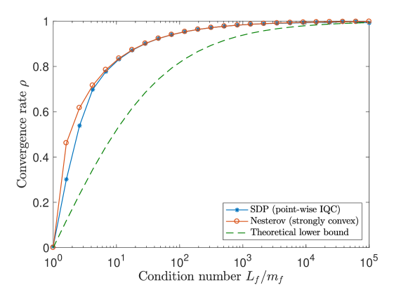
Figure 2: Comparison of rate bounds in Nesterov’s method for different ratios $\kappa_{f}=L_{f}/m_{f}$ using the parameter selection $h=1/L_{f}$ and $\beta=\frac{\sqrt{\kappa_{f}}-1}{\sqrt{\kappa_{f}}+1}$. For this parameter selection, the analytical rate bound is $\rho=\sqrt{1-\frac{1}{\sqrt{\kappa_{f}}}}$ [23].

4.2 Numerical bounds for exponential rates

We could also use the results of Theorem 3.1 to search for the parameters $(a_{k},P_{k})$ numerically. This approach is particularly efficient for time-invariant algorithms with exponential convergence. Under these assumptions, the sequence of LMIs in (3.7) collapses into the single LMI in (3.16), which no longer depends on the iteration index $k$. We can then use this LMI to find the exponential decay rate numerically. Explicitly, the matrix inequality (3.16) is an LMI in $(a_{0},P_{0},\lambda_{0})$ for a fixed $\rho^{2}$. We can therefore use a bisection search aiming to find the smallest value of the convergence rate $\rho$ that satisfies (3.16) for some $(a_{0},P_{0},\lambda_{0})$. Notice that the LMI in (3.16) is homogeneous in its decision variables. We can therefore assume $\lambda_{0}=1$, without loss of generality.

In Figure 2, we compare the numerical rate bounds with the theoretical lower bound and the analytical rate bound of Nesterov’s method with the parameter selection $h=1/L_{f}$ and $\beta={(\sqrt{\kappa_{f}}-1)}/{(\sqrt{\kappa_{f}}+1)}$ [23]. We observe that, the SDP yields slightly better bounds than the analytical rate bound.

We remark that, in [19] the authors make use of quadratic Lyapunov functions and “off-by-one” IQCs to obtain numerical rate bounds for strongly convex problems. They have shown that pointwise IQCs alone exhibit crude bounds and the use of off-by-one IQCs improve the numerical solutions greatly. In contrast, we have utilized nonquadratic Lyapunov functions and pointwise IQCs, which yield nonconservative rate bounds. This nonconservatism is due to the inclusion of the term $a_{k}(F(x_{k})-F(x_{\star}))$ in the Lyapunov function. We conjecture that, by using off-by-one IQCs or other IQCs developed in [19] in our Lyapunov framework, we can further improve the numerical bounds.

4.3 Numerical bounds for subexponential rates

For time-varying algorithms and nonstrongly convex functions, the convergence rate is subexponential and the LMI (3.7) becomes dependent on the iteration number. In this case, a numerical approach amounts to solving an infinite sequence of LMIs to find a rate-generating sequence $\{a_{k}\}$. Nevertheless, we can truncate the sequence of LMIs in order to obtain rate bounds for a finite number of iterations. Specifically, for a given $N>0$, we consider the following SDP:

(4.22) $${\mbox{maximize \ \ }}\ a_{N}$$

subject tofor $$k=0,1,\cdots,N-1$$:

$$\qquad\qquad\quad\ M_{k}^{0}+a_{k}M_{k}^{1}+(a_{k+1}-a_{k})M_{k}^{2}+\sigma_{k}M_{k}^{3}\preceq 0,$$

$$\quad\qquad\quad\quad\ a_{k+1}\geq a_{k},\quad\sigma_{k}\geq 0,\quad P_{k}\succeq 0.$$

with decision variables $\{(a_{k},P_{k},\sigma_{k})\}_{k=1}^{N}$. Denoting the optimal solution of (4.22) by $a^{\star}_{N}$, Theorem 3.1 immediately implies

(4.23) $$f(x_{N})-f(x_{\star})\leq\dfrac{V_{0}(x_{0},\xi_{0})}{a^{\star}_{N}}.$$

In other words, (4.22) searches for the smallest upper bound on the $N$-th (last) iterate suboptimality, subject to the stability constraint imposed by LMI (3.7). Notice that (4.22) is homogeneous in the decision variables. To get a sensible problem, we must normalize the variables by, for example, requiring all of them to add up to a positive constant. Furthermore, the $k$-th LMI in (4.22) is a function of $a_{k}$, $a_{k+1}$, $P_{k}$, $P_{k+1}$, and $\sigma_{k}$. This implies the SDP is banded with a fixed bandwidth independent of $N$, the number of iterations. We can exploit this sparsity structure in solving the SDP efficiently. For instance, for the Nesterov’s method and $N=10^{3}$ iterations, solving the SDP takes less than 10 seconds to solve with an off-the-shelf solver.

In Figure 3, we plot numerical rate bounds obtained by solving (4.22) for the Nesterov’s accelerated method with the parameter selection given in (4.18). We also plot the analytical rate bound given in (4.21). We observe that the numerical rate bound coincides with the analytical rate.

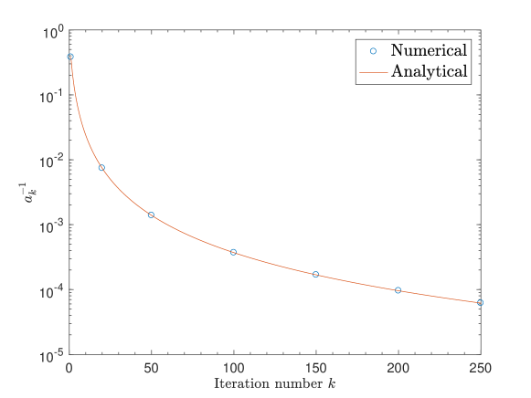
Figure 3: Comparison of rate bounds obtained by numerically solving the SDP in (4.22) and analytical rate bounds for the Nesterov’s accelerated method with the parameter selection given in (4.18).

5 Composite optimization problems

In this section, we consider composite optimization problems of the form

(5.1) $$\mathcal{X}_{\star}=\mathrm{argmin}_{x\in\mathbb{R}^{d}}\{F(x)=f(x)+g(x)\},$$

where $f\colon\mathbb{R}^{d}\to\mathbb{R}$ is differentiable CCP, while $g\colon\mathbb{R}^{d}\to\mathbb{R}\cup\{+\infty\}$ is nondifferentiable and CCP. We assume the optimal solution set $\mathcal{X}_{\star}$ is nonempty and closed, and the optimal value $F(x_{\star})$ is finite. Under these assumptions, the optimality condition for (5.1) is given by

(5.2) $$\mathcal{X}_{\star}=\{x_{\star}\in\mathrm{dom}\,f\cap\mathrm{dom}\,g\colon 0\in\nabla f(x_{\star})+\partial g(x_{\star})\}.$$

Formally, the objective function in (5.1) is nonsmooth and subgradient methods are very slow. Splitting methods such as proximal algorithms circumvent this issue by exploiting the special structure of the objective function to achieve comparable convergence rates to their counterparts in smooth programming. In this section, we analyze proximal algorithms using Theorem 3.1. To this end, we first show that we can represent these algorithms in the canonical form (2.1), where the feedback nonlinearity $\phi$ is the generalized gradient mapping of $F$. By deriving the proximal counterpart of Lemma 4.1, we can then immediately apply Theorem 3.1 to proximal algorithms.

5.1 Generalized gradient mapping

Let $g\colon\mathbb{R}^{d}\to\mathbb{R}\cup\{+\infty\}$ be a CCP function. The proximal operator $\Pi_{g,h}\colon\mathbb{R}^{d}\to\mathbb{R}^{d}$ of $g$ with parameter $h>0$ is defined as

(5.3) $$\Pi_{g,h}(x)=\mathrm{argmin}_{y\in\mathbb{R}^{d}}\ \{g(y)+\dfrac{1}{2h}\|y-x\|_{2}^{2}\}.$$

For the composite function in (5.1), we define the generalized gradient mapping $\phi_{h}\colon\mathbb{R}^{d}\to\mathbb{R}^{d}$ as

(5.4) $$\phi_{h}(x)=\dfrac{1}{h}(x-\Pi_{g,h}(x-h\nabla f(x))),\ h>0.$$

with $\mathrm{dom}\,\phi_{h}=\mathrm{dom}\,f$. Notice that when $g(x)\equiv 0$ (so that $\Pi_{g,h}(x)=x$), the generalized gradient mapping simplifies to the gradient function $\nabla f$. Furthermore, we have that $\phi_{h}(x_{\star})=0$ for $x_{\star}\in\mathcal{X}_{\star}$, i.e., $\phi_{h}$ vanishes at optimality. In the following proposition, we characterize several properties of $\phi_{h}$, which will prove useful.

Proposition 5.1

Consider the composite function $F=f+g$ with $f\!\in\!\mathcal{F}(m_{f},L_{f})$ and $g\in\mathcal{F}(0,\infty)$. Correspondingly, define the generalized gradient mapping $\phi_{h}$ of $F$ as in (5.4) .

1. $\phi_{h}$ satisfies the pointwise IQC defined by $(Q_{\phi_{h}},x_{\star},\phi_{h}(x_{\star}))$, where $Q_{\phi_{h}}$ is given by

   (5.5) $$Q_{\phi_{h}}=\begin{bmatrix}\dfrac{1}{2h}(\gamma_{f}^{2}-1)&\dfrac{1}{2}\\ \dfrac{1}{2}&-\dfrac{h}{2}\end{bmatrix}\!\otimes I_{d},$$

   with $\gamma_{f}=\max\{|1-hL_{f}|,|1-hm_{f}|\}$.

2. The following inequality

   (5.6) $$F(y\!-\!h\phi_{h}(y))\!-\!F(x)\leq \phi_{h}(y)^{\top}(y\!-\!x)\!-\!\dfrac{m_{f}}{2}\|y\!-\!x\|_{2}^{2}+(\frac{1}{2}L_{f}h^{2}\!-\!h)\|\phi_{h}(y)\|_{2}^{2},$$

   holds for all $h\geq 0$ and $x,y\in\mathrm{dom}\,F$.

3. $\phi_{h}(x_{\star})=0$ if and only if $x_{\star}\in\mathrm{argmin}\ F(x)$.

Proof 5.2

See Appendix B.

5.2 Proximal algorithms

Using the definition of generalized gradient mapping in (5.4), we can represent proximal algorithms with the same state-space structure as in (2.1), where the feedback nonlinearity is $\phi=\phi_{h}$. For example, the Nesterov’s accelerated proximal gradient method is defined by

(5.7) $$x_{k+1} =\Pi_{g,h}(y_{k}-h\nabla f(y_{k})),$$

$$y_{k} =x_{k}+\beta_{k}(x_{k}-x_{k-1}),$$

which, by using (5.4), can be rewritten as

(5.8) $$x_{k+1} =x_{k}+\beta_{k}(x_{k}-x_{k-1})-h\phi_{h}(y_{k}),$$

$$y_{k} =x_{k}+\beta_{k}(x_{k}-x_{k-1}).$$

By defining the state vector $\xi_{k}=[x_{k-1}^{\top}\ x_{k}^{\top}]^{\top}\in\mathbb{R}^{2d}$, the corresponding state-space matrices $(A_{k},B_{k},C_{k})$ are given by

(5.13) $$\left[\begin{array}[]{c|c}A_{k}&B_{k}\\ \hline\cr C_{k}&0\end{array}\right]=\left[\begin{array}[]{c|c}\begin{matrix}0&I_{d}\\ -\beta_{k}I_{d}&(\beta_{k}+1)I_{d}\end{matrix}&\begin{matrix}0\\ -hI_{d}\end{matrix}\\ \hline\cr\begin{matrix}-\beta_{k}I_{d}&(\beta_{k}+1)I_{d}\end{matrix}&0\end{array}\right].$$

Recall the assumption that the sequences $\{x_{k}\}$ and $\{y_{k}\}$ converge to the same fixed point in the optimal set. Since $\phi_{h}$ is zero at optimality, we must therefore have that $\phi_{h}(y_{\star})=\phi_{h}(x_{\star})=0$. In other words, the fixed points satisfy

(5.14) $$\xi_{\star}=A_{k}\xi_{\star},\quad y_{\star}=C_{k}\xi_{\star},\quad u_{\star}=\phi_{h}(y_{\star})=0,\quad x_{\star} =E_{k}\xi_{\star}=y_{\star},\quad\mbox{for all }k.$$

Having characterized the generalized gradient mapping with quadratic constraints, we are now ready to develop the proximal counterpart of Lemma 4.1.

Lemma 5.3

Let $x_{\star}\in\mathrm{argmin}\ F(x)$ be a minimizer of $F=f+g$ with a finite optimal value $F(x_{\star})$, where $f\in\mathcal{F}(m_{f},L_{f})$ and $g\in\mathcal{F}(0,\infty)$. Consider a proximal first-order algorithm in the state-space form (2.1) with $\phi=\phi_{h}$ defined as in (5.4). Suppose the fixed points $(\xi_{\star},u_{\star},y_{\star},$ $x_{\star})$ satisfy

(5.15) $$\xi_{\star}=A_{k}\xi_{\star},\ \ y_{\star}=C_{k}\xi_{\star},\ \ u_{\star}=\phi_{h}(y_{\star})=0,\ \ x_{\star}=E_{k}\xi_{\star}=y_{\star}\quad\mbox{for all }k.$$

Then the following inequalities hold for all $k$.

(5.16a) $$F(x_{k+1})-F(x_{k}) \leq e_{k}^{\top}M_{k}^{1}e_{k},$$

(5.16b) $$F(x_{k+1})-F(x_{\star}) \leq e_{k}^{\top}M_{k}^{2}e_{k},$$

(5.16c) $$0 \leq e_{k}^{\top}M_{k}^{3}e_{k},$$

where $e_{k}=[(\xi_{k}-\xi_{\star})^{\top}\ (u_{k}-u_{\star})^{\top}]^{\top}$ and $M_{k}^{1},M_{k}^{2},M_{k}^{3}$ are given by

(5.17) $$M_{k}^{1}\! =\begin{bmatrix}C_{k}\!-\!E_{k}&0\\ 0&I_{d}\end{bmatrix}^{\top}\begin{bmatrix}-\frac{m_{f}}{2}&\frac{1}{2}\\ \frac{1}{2}&(\frac{1}{2}L_{f}h^{2}\!-\!h)\end{bmatrix}\begin{bmatrix}C_{k}\!-\!E_{k}&0\\ 0&I_{d}\end{bmatrix},$$

$$M_{k}^{2} =\begin{bmatrix}C_{k}&0\\ 0&I_{d}\end{bmatrix}^{\top}\begin{bmatrix}-\frac{m_{f}}{2}&\frac{1}{2}\\ \frac{1}{2}&(\frac{1}{2}L_{f}h^{2}\!-\!h)\end{bmatrix}\begin{bmatrix}C_{k}&0\\ 0&I_{d}\end{bmatrix},$$

$$M_{k}^{3} =\begin{bmatrix}C_{k}&0\\ 0&I_{d}\end{bmatrix}^{\top}Q_{\phi_{h}}\begin{bmatrix}C_{k}&0\\ 0&I_{d}\end{bmatrix}.$$

Proof 5.4

See Appendix C.

Remark 5.5

In [19], the authors use a different block diagonal representation of proximal algorithms, in which the linear component is in parallel feedback connections with the gradient function $\nabla f$, as well as the subdifferential operator $\partial g$. Then, each nonlinear block is described by its corresponding IQC, i.e., the IQC of gradient mappings and subdifferential operators. In contrast, we collectively represent all the nonlinearities in a single feedback component (the generalized gradient mapping), whose IQC is given in Lemma 5.1.

In the following, we use Lemma 5.3 in conjunction with Theorem 3.1 to analyze the proximal gradient method and the proximal variant of Nesterov’s accelerated method.

5.2.1 Proximal gradient method

The classical proximal gradient method is defined by the recursion

(5.18) $$x_{k+1}=\Pi_{hg}(x_{k}-h\nabla f(x_{k})),$$

which, by using the definition of the generalized gradient mapping in (5.4), can be written as

(5.19) $$x_{k+1}=x_{k}-h\phi_{h}(x_{k}).$$

The state-space matrices are therefore given by $(A_{k},B_{k},C_{k},E_{k})=(I_{d},-hI_{d},I_{d},I_{d})$. By selecting $P_{k}=p_{k}I_{d},\ p_{k}\geq 0$, the matrices $M_{k}^{i}\ i=0,1,2,3$ are given by

(5.20a) $$M_{k}^{0} =\begin{bmatrix}p_{k+1}\!-\!p_{k}&-hp_{k+1}\\ -hp_{k+1}&h^{2}p_{k+1}\end{bmatrix}\otimes I_{d},$$

(5.20b) $$M_{k}^{1} \!=\!\begin{bmatrix}0\!&\!0\\ 0\!&\!\frac{1}{2}(L_{f}h^{2}\!-\!2h)\end{bmatrix}\otimes I_{d},$$

(5.20c) $$M_{k}^{2} =\begin{bmatrix}-\frac{1}{2}m_{f}&\frac{1}{2}\\ \frac{1}{2}&\frac{1}{2}(L_{f}h^{2}-2h)\end{bmatrix}\otimes I_{d},$$

(5.20d) $$M_{k}^{3} =\begin{bmatrix}\frac{1}{2h}(\gamma_{f}^{2}-1)&\frac{1}{2}\\ \frac{1}{2}&-\frac{h}{2}\end{bmatrix}\!\otimes I_{d},$$

where $\gamma_{f}=\max\{|1-hL_{f}|,|1-hm_{f}|$.

Strongly Convex Case. We first consider the selection $a_{k}\equiv 0$ for strongly convex settings. Then the LMI (5.20) simplifies to

$$\begin{bmatrix}p_{k+1}\!-\!p_{k}&-hp_{k+1}\\ -hp_{k+1}&h^{2}p_{k+1}\end{bmatrix}+\sigma_{k}\begin{bmatrix}\frac{\gamma_{f}^{2}-1}{2h}&\frac{1}{2}\\ \frac{1}{2}&-\frac{h}{2}\end{bmatrix}\leq 0.$$

It can be verified that the above LMI is equivalent to the conditions

$$\sigma_{k}/(2h)\leq p_{k}/\gamma_{f}^{2},\quad p_{k+1}-p_{k}\leq\sigma_{k}(1-\gamma_{f}^{2})/(2h).$$

These two conditions together imply $p_{k+1}\leq p_{k}/\gamma_{f}^{2}$. Therefore, we can write $p_{k}=\gamma_{f}^{-2k}p_{0},\ p_{0}>0$. Using the bound (3.20), we can establish the bound

$$\|x_{k}\!-\!x_{\star}\|_{2}^{2}\leq\left(\max\{|1\!-\!hL_{f}|,|1\!-\!hm_{f}|\}\right)^{2k}\|x_{0}\!-\!x_{\star}\|_{2}^{2}.$$

On the other hand, setting $p_{k}\equiv 0$ in (5.20) yields the LMI

$$\begin{bmatrix}-\dfrac{m_{f}}{2}(a_{k+1}-a_{k})&\dfrac{a_{k+1}-a_{k}}{2}\\ \dfrac{a_{k+1}-a_{k}}{2}&(\dfrac{L_{f}h^{2}}{2}-h)a_{k+1}\end{bmatrix}\preceq 0.$$

Omitting the details, we obtain from the above LMI that $a_{k+1}\leq\rho^{-2}a_{k}$ and $0\leq h\leq 2/L_{f}$, where $\rho^{2}=1+m_{f}(L_{f}h^{2}-2h)$. Substituting $a_{k}$ in (3.17) yields the bound

$$F(x_{k})\!-\!F(x_{\star})\leq(1+m_{f}(L_{f}h^{2}\!-\!2h))^{k}(F(x_{0})-F(x_{\star})).$$

In particular, the optimal decay rate is attained at $h=1/L_{f}$, and is equal to $\rho=1-m_{f}/L_{f}$.

Convex Case. When the differentiable component of the objective is convex ($m_{f}=0$), we select $p_{k}=p>0,\sigma_{k}=\sigma$ in (5.20) to arrive at the LMI

$$\begin{bmatrix}\dfrac{\sigma}{2h}(\gamma_{f}^{2}-1)&\dfrac{1}{2}(a_{k+1}-a_{k}-2ph+\sigma)\\ \dfrac{1}{2}(a_{k+1}-a_{k}-2ph+\sigma)&(\dfrac{L_{f}h^{2}}{2}-h)a_{k+1}+ph^{2}-\dfrac{\sigma h}{2}\end{bmatrix}\preceq 0.$$

To further simplify the LMI, we take $\sigma=0$. Then the LMI enforces that

$$a_{k+1}=a_{k}+2ph,\quad a_{0}\geq 0,\quad(L_{f}h^{2}/2-h)(a_{k+1})+ph^{2}\leq 0$$

Solving for $a_{k}$ leads to

$$F(x_{k})-F(x_{\star})\leq\dfrac{a_{0}(F(x_{0})-F(x_{\star}))+p\|x_{0}-x_{\star}\|_{2}^{2}}{a_{0}+2phk}.$$

In particular, if $a_{0}=0$, then it must hold that $0\leq h\leq 1/L_{f}$, and we recover the convergence result in [3, Theorem 3.1].

5.2.2 Accelerated proximal gradient method

Consider the proximal variant of Nesterov’s accelerated method outlined in (5.7), for which the state-space matrices are given in (5.13). Making use of Lemma 5.3, the matrices $M_{k}^{i}\ i\in\{0,1,2,3\}$ read as

(5.21) $$M_{k}^{0} =\begin{bmatrix}A_{k}^{\top}P_{k+1}A_{k}\!-\!P_{k}&A_{k}^{\top}P_{k+1}B_{k}\\ B_{k}^{\top}P_{k+1}A_{k}&B_{k}^{\top}P_{k+1}B_{k}\end{bmatrix},$$

$$M_{k}^{1} =\begin{bmatrix}-\frac{1}{2}m_{f}\beta_{k}^{2}&\frac{1}{2}m_{f}\beta_{k}^{2}&-\frac{1}{2}\beta_{k}\\ \frac{1}{2}m_{f}\beta_{k}^{2}&-\frac{1}{2}m_{f}\beta_{k}^{2}&\frac{1}{2}\beta_{k}\\ -\frac{1}{2}\beta_{k}&\frac{1}{2}\beta_{k}&\frac{1}{2}L_{f}h^{2}-h\end{bmatrix},$$

$$M_{k}^{2} =\begin{bmatrix}-\frac{1}{2}m_{f}\beta_{k}^{2}&\frac{1}{2}m_{f}\beta_{k}(\beta_{k}+1)&-\frac{1}{2}\beta_{k}\\ \frac{1}{2}m_{f}\beta_{k}(\beta_{k}+1)&-\frac{1}{2}m_{f}(\beta_{k}+1)^{2}&\frac{1}{2}(\beta_{k}+1)\\ -\frac{1}{2}\beta_{k}&\frac{1}{2}(\beta_{k}+1)&\frac{1}{2}L_{f}h^{2}-h\end{bmatrix},$$

$$M_{k}^{3} =\begin{bmatrix}-\beta_{k}I_{d}&0\\ (1+\beta_{k})I_{d}&0\\ 0&I_{d}\end{bmatrix}\begin{bmatrix}\frac{1}{2h}(\gamma_{f}^{2}-1)I_{d}&\frac{1}{2}I_{d}\\ \frac{1}{2}I_{d}&-\frac{h}{2}I_{d}\end{bmatrix}\begin{bmatrix}-\beta_{k}I_{d}&(1+\beta_{k})I_{d}&0\\ 0&0&I_{d}\end{bmatrix}.$$

Observe that the matrices $M_{k}^{0},M_{k}^{1}$, and $M_{k}^{2}$ are precisely the same as those of Nesterov’s method without proximal operation. The only difference is in $M_{k}^{3}$. As a result, by setting $\sigma_{k}=0$ (the coefficient of $M_{k}^{3}$) in the LMI (3.7), the analysis of Nesterov’s accelerated method in $\S$4.1.2 immediately applies to the proximal variant [11].

Remark 5.6 (Gradient methods with projection)

For the case that $g(x)=\mathbb{I}_{\mathcal{X}}(x)$ is the indicator function of a nonempty, closed convex set $\mathcal{X}\subset\mathbb{R}^{d}$, the proximal operator $\Pi_{g,h}$ reduces to projection onto $\mathcal{X}$. Due to projection, we must have $x_{k}\in\mathcal{X}$ for all $k$, implying $g(x_{k})=0$. Therefore, the convergence result of Theorem 3.1 holds for the suboptimality $f(x_{k})-f(x_{\star})$.

6 Further topics

In this section, we consider further applications of the developed framework, namely, calculus of IQCs for various operators in optimization, continuous-time models and, more importantly, algorithm design.

6.1 Calculus of IQCs

We now describe some operations on mappings from an IQC perspective, namely, inversion, affine operations, and function composition. These operations form a calculus that is useful for determining IQCs for commonly used nonlinear operators in optimization algorithms, such as proximal operators, projection operators, reflection operators, etc., and their compositions.

It directly follows from the definition of pointwise IQCs in (3.21) that if $\phi$ satisfies multiple pointwise IQCs defined by $(Q_{\phi,i},$ $x_{\star},$ $\phi(x_{\star}))$, $i=1,2,\ldots,\ell$, it also satisfies the pointwise IQC defined by $(\sum_{i=1}^{\ell}\!\sigma_{i}Q_{\phi,i}$ $,x_{\star},$ $\phi(x_{\star}))$, where $\sigma_{i}\geq 0,\ i=1,2,\ldots,\ell$. Further, $\phi$ also satisfies the IQC defined by $(Q,x_{\star},\phi(x_{\star}))$ for any $Q\succeq Q_{\phi}$. In the next two lemmas, we study the effect of inversion and affine transformation on IQCs.

Lemma 6.1 (IQC for inversion)

Consider an invertible map $\phi\colon\mathbb{R}^{d}\to\mathbb{R}^{d}$ with $\phi^{-1}(\mathrm{dom}\,\phi)\subseteq\mathrm{dom}\,\phi$ satisfying the pointwise IQC defined by $(Q_{\phi},x_{\star},\phi(x_{\star}))$. Then, the inverse map $\phi^{-1}\colon\mathbb{R}^{d}\to\mathbb{R}^{d}$ satisfies the pointwise IQC defined by $(Q_{\phi^{-1}}$,$\phi(x_{\star})$,$x_{\star})$, where

(6.1) $$Q_{\phi^{-1}}=\begin{bmatrix}0&I_{d}\\ I_{d}&0\end{bmatrix}Q_{\phi}\begin{bmatrix}0&I_{d}\\ I_{d}&0\end{bmatrix}.$$

Proof 6.2

By the substitution $x\leftarrow\phi^{-1}(x)$ in (3.21), we obtain

(6.2) $$\begin{bmatrix}\phi^{-1}(x)-\phi^{-1}(x_{\star})\\ x-x_{\star}\end{bmatrix}^{\top}Q_{\phi}\,\begin{bmatrix}\phi^{-1}(x)-\phi^{-1}(x_{\star})\\ x-x_{\star}\end{bmatrix}\geq 0.$$

Further, we have

(6.3) $$\begin{bmatrix}\phi^{-1}(x)-\phi^{-1}(x_{\star})\\ x-x_{\star}\end{bmatrix}=\begin{bmatrix}0&I_{d}\\ I_{d}&0\end{bmatrix}\begin{bmatrix}x-x_{\star}\\ \phi^{-1}(x)-\phi^{-1}(x_{\star})\end{bmatrix}.$$

Substituting (6.3) in (6.2) yields (6.1).

Lemma 6.3 (IQC for affine operations)

Consider a map $\phi\colon\mathbb{R}^{d}\to\mathbb{R}^{d}$ satisfying the pointwise IQC defined by $(Q_{\phi},x_{\star},\phi(x_{\star}))$. Correspondingly, define the map $\psi(x)=S_{2}x+S_{1}\phi(S_{0}x)$ with $S_{0}(\mathrm{dom}\,\phi)\subseteq\mathrm{dom}\,\phi$, where $S_{0},S_{1},S_{2}\in\mathbb{R}^{d\times d}$, and $S_{1}$ is invertible. Then, $\psi$ satisfies the pointwise IQC defined by $(Q_{\psi},x_{\star},\psi(x_{\star}))$, where

(6.4) $$Q_{\psi}=\begin{bmatrix}S_{0}^{\top}&-(S_{1}^{-1}S_{2})^{\top}\\ 0&S_{1}^{-1}\end{bmatrix}Q_{\phi}\begin{bmatrix}S_{0}&0\\ -S_{1}^{-1}S_{2}&(S_{1}^{-1})^{\top}\end{bmatrix}.$$

Proof 6.4

By the substitution $x\leftarrow S_{0}x$ in (3.21), we obtain

(6.5) $$\begin{bmatrix}S_{0}x-S_{0}x_{\star}\\ \phi(S_{0}x)-\phi(S_{0}x_{\star})\end{bmatrix}^{\top}Q_{\phi}\,\begin{bmatrix}S_{0}x-S_{0}x_{\star}\\ \phi(S_{0}x)-\phi(S_{0}x_{\star})\end{bmatrix}\geq 0.$$

Further, since $\psi(x)=S_{2}x+S_{1}\phi(S_{0}x)$, we have

(6.6) $$\begin{bmatrix}S_{0}x-S_{0}x_{\star}\\ \phi(S_{0}x)-\phi(S_{0}x_{\star})\end{bmatrix}=\begin{bmatrix}S_{0}&0\\ -S_{1}^{-1}S_{2}&S_{1}^{-1}\end{bmatrix}\begin{bmatrix}x-x_{\star}\\ \psi(x)-\psi(x_{\star})\end{bmatrix}.$$

Substituting (6.6) in (6.5) yields (6.4).

Finally, we study the composition of mappings. Specifically, consider the cascade connection of two mappings $\phi_{1},\phi_{2}\colon\mathbb{R}^{d}\to\mathbb{R}^{d},\ i=1,2$ as in Figure 4, where $y=\phi_{1}(x)$ and $z=\phi_{2}(y)$. Further assume $\phi_{1}$ and $\phi_{2}$ satisfy pointwise IQCs defined by $(Q_{\phi_{1}},x_{\star},y_{\star})$ and $(Q_{\phi_{2}},y_{\star},z_{\star})$, respectively. By definition, these mappings impose the following quadratic constraints on the pairs $(x,y)$ and $(y,z)$:

$$\begin{bmatrix}x-x_{\star}\\ y-y_{\star}\end{bmatrix}^{\top}Q_{\phi_{1}}\,\begin{bmatrix}x-x_{\star}\\ y-y_{\star}\end{bmatrix}\geq 0,\quad\begin{bmatrix}y-y_{\star}\\ z-z_{\star}\end{bmatrix}^{\top}Q_{\phi_{2}}\,\begin{bmatrix}y-y_{\star}\\ z-z_{\star}\end{bmatrix}\geq 0.$$

These two constraints separately define a quadratic constraint on the triple $(x,y,z)$, which can be encapsulated in a single constraint, as follows:

(6.7a) $$\begin{bmatrix}x-x_{\star}\\ y-y_{\star}\\ z-z_{\star}\end{bmatrix}^{\top}Q_{\psi}\begin{bmatrix}x-x_{\star}\\ y-y_{\star}\\ z-z_{\star}\end{bmatrix}\geq 0,$$

where $$Q_{\psi}\in\mathbb{S}^{3d}$$ is given by

(6.7b) $$Q_{\psi}=\begin{bmatrix}I_{d}&0\\ 0&I_{d}\\ 0&0\end{bmatrix}\sigma_{1}Q_{\phi_{1}}\begin{bmatrix}I_{d}&0&0\\ 0&I_{d}&0\end{bmatrix}+\begin{bmatrix}0&0\\ I_{d}&0\\ 0&I_{d}\end{bmatrix}\sigma_{2}Q_{\phi_{2}}\begin{bmatrix}0&I_{d}&0\\ 0&0&I_{d}\end{bmatrix},$$

with $\sigma_{1},\sigma_{2}\geq 0$. The quadratic constraint in (6.7a) follows by substituting (6.7b) into (6.7a). In the language of IQCs, we can say that the map $\psi=[\phi_{1}^{\top}\ (\phi_{2}\circ\phi_{1})^{\top}]^{\top}$ $\colon\mathbb{R}^{d}\to\mathbb{R}^{2d}$ satisfies the pointwise IQC defined by $(Q_{\psi},x_{\star},\psi(x_{\star}))$, where $Q_{\psi}$ is given by (6.7b).

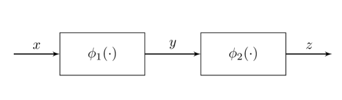
Figure 4: Cascade connection of two nonlinear mappings.

We remark that the above treatment can be extended to multiple compositions. Specifically, for $\ell$ mappings in a cascade connection, the corresponding $\ell$ individual IQCs can be grouped into a single quadratic constraint on the concatenated vector of the input-output signals.

6.1.1 Proximal operators

Recall the definition of proximal operator for $f:\mathbb{R}^{d}\to\mathbb{R}\cup\{+\infty\}$:

(6.8) $$\Pi_{f,h}(x)=\mathrm{argmin}_{y\in\mathbb{R}^{d}}\{f(y)+\dfrac{1}{2h}\|y-x\|_{2}^{2}\}.$$

To characterize $\Pi_{f,h}$ from an IQC perspective, we note that for any given $x\in\mathrm{dom}\,f$, a necessary condition for optimality in (6.8) is that

(6.9) $$0\in\partial f(\Pi_{g,h}(x))+\dfrac{1}{h}(\Pi_{f,h}(x)-x),\ \mbox{for all }x\in\mathrm{dom}\,f,$$

which is an implicit equation on $\Pi_{f,h}(x)$. In the next proposition, we show how to obtain a quadratic constraint for the proximal operator $\Pi_{f,h}$ from that of the subgradient $T_{f}$ by using the necessary optimality condition (6.9) that couples these two operators.

Proposition 6.5 (IQCs for proximal operators)

Let $f\colon\mathbb{R}^{d}\to\mathbb{R}\cup\{+\infty\}$ be a closed proper function whose subgradient $T_{f}$ satisfies the pointwise IQC defined by $(Q_{f},x_{\star},T_{f}(x_{\star}))$, where $T_{f}(x_{\star})\in\partial f(x_{\star})$. Then, the proximal operator $\Pi_{hf}$ satisfies the pointwise IQC defined by $(Q_{\Pi_{hf}},x_{\star},\Pi_{hf}(x_{\star}))$, where

(6.10) $$Q_{\Pi_{hf}}=\begin{bmatrix}0&h^{-1}I_{d}\\ I_{d}&-h^{-1}I_{d}\end{bmatrix}Q_{f}\begin{bmatrix}0&I_{d}\\ h^{-1}I_{d}&-h^{-1}I_{d}\end{bmatrix}.$$

Proof 6.6

Suppose $T_{f}(x)\in\partial f(x)$ ($T_{f}(x)=\nabla f(x)$ when $f$ is differentiable) satisfies the pointwise IQC defined by $(Q_{f},x_{\star},T_{f}(x_{\star}))$. By the substitution $x\leftarrow\Pi_{hf}(x)$ and $x_{\star}\leftarrow\Pi_{hf}(x_{\star})$ in (3.21), we obtain

(6.11) $$\begin{bmatrix}\Pi_{hf}(x)-\Pi_{hf}(x_{\star})\\ T_{f}(\Pi_{hf}(x))-T_{f}(\Pi_{hf}(x_{\star}))\end{bmatrix}^{\top}Q_{f}\,\begin{bmatrix}\Pi_{hf}(x)-\Pi_{hf}(x_{\star})\\ T_{f}(\Pi_{hf}(x))-T_{f}(\Pi_{hf}(x_{\star}))\end{bmatrix}\geq 0.$$

On the other hand, by the optimality condition (6.9), we have $T_{f}(\Pi_{hf}(x))=\frac{1}{h}(x-\Pi_{hf}(x))$. Substituting this into (6.11), we obtain

(6.12) $$\begin{bmatrix}\Pi_{hf}(x)-\Pi_{hf}(x_{\star})\\ \dfrac{1}{h}(x-x_{\star})-\dfrac{1}{h}(\Pi_{hf}(x)-\Pi_{hf}(x_{\star}))\end{bmatrix}^{\top}\!Q_{f}\!\begin{bmatrix}\Pi_{hf}(x)-\Pi_{hf}(x_{\star})\\ \dfrac{1}{h}(x-x_{\star})-\dfrac{1}{h}(\Pi_{hf}(x)-\Pi_{hf}(x_{\star}))\end{bmatrix}\geq 0.$$

Further, we can write

(6.13) $$\begin{bmatrix}\Pi_{hf}(x)-\Pi_{hf}(x_{\star})\\ \dfrac{1}{h}(x-x_{\star})-\dfrac{1}{h}(\Pi_{hf}(x)-\Pi_{hf}(x_{\star}))\end{bmatrix}=\begin{bmatrix}0&I_{d}\\ \dfrac{1}{h}I_{d}&-\dfrac{1}{h}I_{d}\end{bmatrix}\begin{bmatrix}x-x_{\star}\\ \Pi_{hf}(x)-\Pi_{hf}(x_{\star})\end{bmatrix}.$$

By substituting (6.13) in (6.12), we will arrive at the desired inequality in (6.10).

Notice that by (6.9), we have that $\Pi_{hf}=(I+h\partial f)^{-1}$. In other words, the proximal operator is obtained by the operations $\partial f\to I+h\partial f\to(I+h\partial f)^{-1}$, i.e., an affine operation on $\partial f$ followed by an inversion. Therefore, for obtaining the IQC of $\Pi_{hf}$ from that of $\partial f$, we can directly use Lemma 6.1 and 6.3 to arrive at an alternative derivation of (6.10).

6.1.2 IQCs for projection operators

The projection operator is the proximal operator $\Pi_{hf}$ for the particular selection $f(x)=\mathbb{I}_{\mathcal{X}}(x)$, where $\mathbb{I}_{\mathcal{X}}$ is the extended-value indicator function of the nonempty closed convex set $\mathcal{X}\subset\mathbb{R}^{d}$ onto which we project. Since $f$ is nondifferentiable and convex in this case, its subgradient operator $T_{f}$ satisfies the pointwise IQC defined by $(Q_{f},x_{\star},T_{f}(x_{\star}))$, where $Q_{f}$ is given by (3.27) with $L_{f}=\infty$. It then follows from Proposition 6.5 that the projection operator $\Pi_{\mathcal{X}}$ satisfies the IQC defined by $(Q_{\Pi_{\mathcal{X}}},x_{\star},\Pi_{\mathcal{X}}(x_{\star}))$, where

(6.14) $$Q_{\Pi_{\mathcal{X}}}=\begin{bmatrix}0&\dfrac{1}{2}\\ \dfrac{1}{2}&-1\end{bmatrix}\otimes I_{d}.$$

This IQC corresponds to the firm nonexpansiveness property of the projection operator [7], which implies the Lipschitz continuity of $\Pi_{\mathcal{X}}$ with Lipschitz parameter equal to one.

6.2 Beyond convexity

The convergence analysis of several algorithms do not make a full use of convexity. In other words, convexity is sufficient for convergence of these algorithms. This has motivated the introduction of function classes that are relaxation of convexity. In this subsection, we briefly discuss some of these classes and how they can be related to the developed framework in this paper. Formally, consider a continuously differentiable function $f\colon$ $\mathbb{R}^{d}\to\mathbb{R}$ that satisfies the following bounds.

(6.15) $$\begin{bmatrix}x-x_{\star}\\ \nabla f(x)\end{bmatrix}^{\top}{R}^{\prime}_{f}\begin{bmatrix}x-x_{\star}\\ \nabla f(x)\end{bmatrix}\leq f(x)-f(x_{\star})\leq\begin{bmatrix}x-x_{\star}\\ \nabla f(x)\end{bmatrix}^{\top}R_{f}\begin{bmatrix}x-x_{\star}\\ \nabla f(x)\end{bmatrix},$$

where $R_{f},R^{\prime}_{f}\in\mathbb{S}^{2d}$ are symmetric matrices and $x_{\star}$ is such that $\nabla f(x_{\star})=0$. It follows from (6.15) that

(6.16) $$\begin{bmatrix}x-x_{\star}\\ \nabla f(x)\end{bmatrix}^{\top}(R_{f}-R^{\prime}_{f})\begin{bmatrix}x-x_{\star}\\ \nabla f(x)\end{bmatrix}\geq 0.$$

Note that since $\nabla f(x_{\star})=0$, the above inequality implies that $\nabla f$ satisfies the pointwise IQC defined by $(R_{f}-R^{\prime}_{f},x_{\star},\nabla f(x_{\star}))$. Several function classes can be written in the form (6.15), where $R_{f}$ and $R^{\prime}_{f}$ differ for each class. We give three examples below.

(Strongly) convex functions. In $\S$3.2.2, we considered IQCs for convex functions. Specifically, the quadratic inequality (3.26) is necessary and sufficient for the inclusion $f\in\mathcal{F}(m_{f},L_{f})$. An equivalent inequality involving function values is [29]

(6.17) $$f(y)\!-\!f(x)\!-\!\nabla f(x)^{\top}(y\!-\!x)\geq\frac{1}{2(L_{f}\!-\!m_{f})}\|\nabla f(y)\!-\!\nabla f(x)\|_{2}^{2}$$

$$\qquad\qquad\qquad\quad+\frac{m_{f}L_{f}}{2(L_{f}\!-\!m_{f})}\|y\!-\!x\|_{2}^{2}\!-\!\dfrac{m_{f}}{L_{f}\!-\!m_{f}}(\nabla f(y)\!-\!\nabla f(x))^{\top}(y-x),$$

If we restrict (6.17) to hold only for the particular selection $(x,y)=(x_{\star},x)$ and $(x,y)=(x,x_{\star})$, we obtain a new class of functions that can be put in the form (6.15) with $R^{\prime}_{f},R_{f}$ given by

(6.18) $${R}^{\prime}_{f} =\begin{bmatrix}\frac{m_{f}L_{f}}{2(L_{f}-m_{f})}&\frac{-m_{f}}{2(L_{f}-m_{f})}\\ \frac{-m_{f}}{2(L_{f}-m_{f})}&\frac{1}{2(L_{f}-m_{f})}\end{bmatrix}\otimes I_{d},\quad{R}_{f}=\begin{bmatrix}\frac{-m_{f}L_{f}}{2(L_{f}-m_{f})}&\frac{L_{f}}{2(L_{f}-m_{f})}\\ \frac{L_{f}}{2(L_{f}-m_{f})}&\frac{-1}{2(L_{f}-m_{f})}\end{bmatrix}\otimes I_{d},$$

Using (6.16), we can conclude

(6.19) $$\begin{bmatrix}x-x_{\star}\\ \nabla f(x)\end{bmatrix}^{\top}\begin{bmatrix}-\frac{m_{f}L_{f}}{m_{f}+L_{f}}I_{d}&\frac{1}{2}I_{d}\\ \frac{1}{2}I_{d}&-\frac{1}{m_{f}+L_{f}}I_{d}\end{bmatrix}\begin{bmatrix}x-x_{\star}\\ \nabla f(x)\end{bmatrix}\geq 0.$$

Note that this quadratic inequality is the same as that of convex functions but only holds when the reference point $x_{\star}$ in the definition of pointwise IQC satisfies $\nabla f(x_{\star})=0$.

Weakly smooth weakly quasiconvex functions. Suppose $f$ is continuously differentiable and satisfies [13]:

(6.20) $$\dfrac{1}{\Gamma_{f}}\|\nabla f(x)\|_{2}^{2}\leq f(x)-f(x_{\star})\leq\dfrac{1}{\tau_{f}}\nabla f(x)^{\top}(x-x_{\star})\quad\text{for all}\ x\in\mathcal{S},$$

where $x_{\star}$ is a global minimum of $f$, and $0<\tau_{f},\Gamma_{f}<\infty$. These inequalities ensure that any point with vanishing gradient is optimal [13], i.e., $\nabla f(x_{\star})=0$. The inequality (6.20) can be put in the form (6.15), where $R^{\prime}_{f},R_{f},$ and $Q_{f}$ are given by

(6.21) $${R}^{\prime}_{f}=\begin{bmatrix}0&0\\ 0&\frac{1}{\Gamma_{f}}\end{bmatrix}\otimes I_{d},\ \ {R}_{f}=\begin{bmatrix}0&\frac{1}{2\tau_{f}}\\ \frac{1}{2\tau_{f}}&0\end{bmatrix}\otimes I_{d},\ \ Q_{f}=\begin{bmatrix}0&\frac{1}{2\tau_{f}}\\ \frac{1}{2\tau_{f}}&-\frac{1}{\Gamma_{f}}\end{bmatrix}\otimes I_{d}.$$

Polyak-$\L{}$ojasiewicz (PL) condition. Suppose $f$ is continuously differentiable and satisfies

(6.22) $$0\leq f(x)-f(x_{\star})\leq\dfrac{1}{2m_{f}}\|\nabla f(x)\|_{2}^{2}\quad\text{for all}\ x\in\mathcal{S},$$

for some $m_{f}>0$. Again, this class can be put in the form (6.15).

6.3 Continuous-time models

There is a close connection between iterative algorithms and discretization of ordinary differential equations (ODE). In fact, many iterative first-order optimization algorithms reduce to their “generative” ODEs by time-scaling and infinitesimal step sizes. In this subsection, we consider convergence analysis of continuous-time models for solving the unconstrained problem in (4.1). Specifically, consider the following continuous-time dynamical system in state-space form:

(6.23) $$\dot{\xi}(t)=A(t)\xi(t)+B(t)u(t),\ \ y(t)=C(t)\xi(t),\ \ u(t)=\nabla f(y(t))\ \ \mbox{for all }t\geq t_{0},$$

where at each continuous time $t\geq t_{0}$, $\xi(t)\in\mathbb{R}^{n}$ is the state, $y(t)\in\mathbb{R}^{d}$ is the output ($d\leq n$), and $u(t)=\nabla f(y(t))$ is the feedback input. We assume (6.23) solves (4.1) asymptotically from all admissible initial conditions, i.e., $y(t)$ satisfies $\lim_{t\to\infty}f(y(t))=f(y_{\star})$, where the optimal point $y_{\star}$ obeys $\nabla f(y_{\star})=0$. Therefore, any fixed point of (6.23) satisfies

(6.24) $$0=A(t)\xi_{\star},\quad y_{\star}=C(t)\xi_{\star},\quad u_{\star}=\nabla f(y_{\star})=0\quad\mbox{for all }t\geq t_{0}.$$

We replicate the convergence analysis of discrete-time models using the Lyapunov function

(6.25) $$V(\xi(t),t)=a(t)(f(y(t))-f(y_{\star}))+(\xi(t)-\xi_{\star})^{\top}P(t)(\xi(t)-\xi_{\star}),$$

where $(\xi(t),y(t))$ satisfies (6.23) and $(\xi_{\star},y_{\star})$ satisfies (6.24). The Lyapunov function is parameterized by $P(t)\in\mathbb{S}_{+}^{n}$, as well as $a(t)\geq 0$. If $a(t)$ and $P(t)$ are such that $\dot{V}(\xi(t),t)\leq 0$, then we could guarantee that $V(\xi(t),t)\leq V(\xi(t_{0}),t_{0})$, which in turn implies

(6.26) $$0\leq f(y(t))-f(y_{\star})\leq V(\xi(t_{0}),t_{0})/a(t)=\mathcal{O}(1/a(t))\quad\mbox{for all }t\geq t_{0}.$$

In other words, $a(t)$ provides a lower bound on the convergence rate. Ideally, we are interested in finding the best bound, which translates into the fastest growing $a(t)$. In the following theorem, we develop an LMI to find such an $a(t)$.

Theorem 6.7

Let $f\in\mathcal{F}(m_{f},L_{f})$ and consider the continuous-time dynamics in (6.23), whose fixed points satisfy (6.24). Suppose there exist a differentiable nondecreasing $a(t)\colon[t_{0},\infty)\to\mathbb{R}_{+}$, a differentiable $P(t)\colon[t_{0},\infty)\to\mathbb{S}_{+}^{n}$, and a continuous $\sigma(t)\colon[t_{0},\infty)\to\mathbb{R}_{+}$ that satisfy

(6.27) $$M_{0}(t)+a(t)M_{1}(t)+\dot{a}(t)M_{2}(t)+\sigma(t)M_{3}(t)\preceq 0\quad\mbox{for all }t\geq t_{0},$$

where

$$M_{0}(t) =\begin{bmatrix}P(t)A(t)\!+\!A(t)^{\top}P(t)\!+\!\dot{P}(t)&P(t)B(t)\\ B(t)^{\top}P(t)&0\end{bmatrix},$$

$$M_{1}(t) =\dfrac{1}{2}\!\begin{bmatrix}0&(C(t)A(t)+\dot{C}(t))^{\top}\\ C(t)A(t)+\dot{C}(t)&C(t)B(t)+B(t)^{\top}C(t)^{\top}\end{bmatrix},$$

$$M_{2}(t) =\begin{bmatrix}C(t)^{\top}&0\\ 0&I_{d}\end{bmatrix}\begin{bmatrix}-\frac{m_{f}}{2}I_{d}&\frac{1}{2}I_{d}\\ \frac{1}{2}I_{d}&0\end{bmatrix}\begin{bmatrix}C(t)&0\\ 0&I_{d}\end{bmatrix},$$

$$M_{3}(t) =\begin{bmatrix}C(t)^{\top}&0\\ 0&I_{d}\end{bmatrix}\begin{bmatrix}-\frac{m_{f}L_{f}}{m_{f}+L_{f}}I_{d}&\frac{1}{2}I_{d}\\ \frac{1}{2}I_{d}&-\frac{1}{m_{f}+L_{f}}I_{d}\end{bmatrix}\begin{bmatrix}C(t)&0\\ 0&I_{d}\end{bmatrix},$$

Then, for any $y(t_{0})\in\mathrm{dom}\,f$, the following inequality holds for all $t\geq t_{0}$.

(6.28) $$f(y(t))-f(y_{\star})\leq\dfrac{a(t_{0})(f(y(t_{0}))\!-\!f(y_{\star}))+(\xi(t_{0})\!-\!\xi_{\star})^{\top}P(t_{0})(\xi(t_{0})\!-\!\xi_{\star})}{a(t)}$$

Proof 6.8

It suffices to show that the LMI condition in (6.27) implies $\dot{V}(\xi(t),t)\leq 0$. The time derivative of the Lyapunov function (6.25) is

(6.29) $$\dot{V}=\dot{a} (f(y)-f(y_{\star}))+a\nabla f(y)^{\top}\dot{y}\!+\!2(\xi-\xi_{\star})^{\top}P\dot{\xi}+(\xi-\xi_{\star})^{\top}\dot{P}(\xi-\xi_{\star}).$$

We have dropped the arguments for notational simplicity. We proceed to bound all the terms in the right-hand side of (6.29), using the assumption $f\in\mathcal{F}(m_{f},L_{f})$. By invoking (strong) convexity, we can write

(6.30) $$f(y)\!-\!f(y_{\star}) \leq\begin{bmatrix}y-y_{\star}\\ \nabla f(y)-\nabla f(y_{\star})\end{bmatrix}^{\top}\begin{bmatrix}-\frac{m_{f}}{2}I_{d}&\frac{1}{2}I_{d}\\ \frac{1}{2}I_{d}&0\end{bmatrix}\,\begin{bmatrix}y-y_{\star}\\ \nabla f(y)-\nabla f(y_{\star})\end{bmatrix}$$

$$=\begin{bmatrix}\xi-\xi_{\star}\\ u-u_{\star}\end{bmatrix}^{\top}\begin{bmatrix}C&0\\ 0&I_{d}\end{bmatrix}^{\top}\begin{bmatrix}-\frac{m_{f}}{2}I_{d}&\frac{1}{2}I_{d}\\ \frac{1}{2}I_{d}&0\end{bmatrix}\begin{bmatrix}C&0\\ 0&I_{d}\end{bmatrix}\,\begin{bmatrix}\xi-\xi_{\star}\\ u-u_{\star}\end{bmatrix}.$$

$$=e^{\top}M_{2}e.$$

where we have defined $e=\begin{bmatrix}(\xi-\xi_{\star})^{\top}&(u-u_{\star})^{\top}\end{bmatrix}$. Further, we can write

(6.31) $$\nabla f(y)^{\top}\dot{y}=(u-u_{\star})^{\top}(CA(\xi-\xi_{\star})+CB(u-u_{\star})+\dot{C}(\xi-\xi_{\star}))$$

$$=\begin{bmatrix}\xi-\xi_{\star}\\ u-u_{\star}\end{bmatrix}^{\top}\begin{bmatrix}0&\frac{1}{2}(CA+\dot{C})^{\top}\\ \frac{1}{2}(CA+\dot{C})&\frac{1}{2}(CB+B^{\top}C^{\top})\end{bmatrix}\begin{bmatrix}\xi-\xi_{\star}\\ u-u_{\star}\end{bmatrix}$$

$$=e^{\top}M_{1}e.$$

where we have used (6.23) and (6.24). Similarly, we can write

(6.32) $$2(\xi-\xi_{\star})^{\top}P\dot{\xi} =\begin{bmatrix}\xi-\xi_{\star}\\ u-u_{\star}\end{bmatrix}^{\top}\begin{bmatrix}PA+A^{\top}P&PB\\ B^{\top}P^{\top}&0\end{bmatrix}\begin{bmatrix}\xi-\xi_{\star}\\ u-u_{\star}\end{bmatrix}=e^{\top}M_{0}e.$$

Finally, since $f\in\mathcal{F}(m_{f},L_{f})$, $\nabla f$ satisfies the quadratic constraint in (3.27). Therefore, we can write

(6.33) $$e^{\top}M_{3}e =\begin{bmatrix}\xi-\xi_{\star}\\ u-u_{\star}\end{bmatrix}^{\top}\begin{bmatrix}C&0\\ 0&I_{d}\end{bmatrix}^{\top}\begin{bmatrix}-\frac{m_{f}L_{f}}{m_{f}+L_{f}}I_{d}&\frac{1}{2}I_{d}\\ \frac{1}{2}I_{d}&-\frac{1}{m_{f}+L_{f}}I_{d}\end{bmatrix}\begin{bmatrix}C&0\\ 0&I_{d}\end{bmatrix}\,\begin{bmatrix}\xi-\xi_{\star}\\ u-u_{\star}\end{bmatrix}$$

$$=\!\begin{bmatrix}y-y_{\star}\\ u-u_{\star}\end{bmatrix}^{\top}\begin{bmatrix}-\frac{m_{f}L_{f}}{m_{f}+L_{f}}I_{d}&\frac{1}{2}I_{d}\\ \frac{1}{2}I_{d}&-\frac{1}{m_{f}+L_{f}}I_{d}\end{bmatrix}\begin{bmatrix}y-y_{\star}\\ u-u_{\star}\end{bmatrix}\geq 0.$$

By substituting (6.30)-(6.32) in (6.29) and rearranging terms, we can write

(6.34) $$\dot{V} \leq e^{\top}\left(M_{0}+aM_{1}+\dot{a}M_{2}\right)e$$

The LMI in (6.27) implies

(6.35) $$M_{0}+aM_{1}+\dot{a}M_{2}\preceq-\sigma M_{3}$$

Multiplying (6.35) on the left and right by $e^{\top}$ and $e$, respectively, and substituting the result back in (6.34) yields

$$\dot{V} \leq-\sigma e^{\top}M_{3}e\leq 0,$$

where the second inequality follows from (6.33). The proof is now complete.

According to Theorem 6.7, we can find the rate generating function $a(t)$ by solving the LMI in (6.27). More precisely, this LMI defines a first-order differential inequality on $a(t)$ whose solutions certify an $\mathcal{O}(1/a(t))$ convergence rate. The best lower bound on the convergence rate (i.e., the fastest growing $a(t)$) can be found by solving the following symbolic optimization problem:

(6.36) $$\underset{\dot{a}(t)\geq 0,\sigma(t)\geq 0}{\mbox{maximize}}\ \dot{a}(t)\ \mbox{subject to}\ \dot{a}(t)M_{0}(t)+a(t)M_{1}(t)+M_{2}(t)+\sigma(t)M_{3}(t)\preceq 0,$$

The optimality condition for (6.36) translates into a first-order differential equation (ODE) on $a(t)$. The solution to this ODE yields the best rate bound that can be certified using the Lyapunov function (6.25). In the following, we specialize the model in (6.23) to the particular case of the gradient flow ($\S$6.3.1) and its accelerated variant ($\S$6.3.2), where we will use Theorem 6.7 to derive the corresponding convergence rates.

6.3.1 Continuous-time gradient flow

Consider the following ODE for solving (4.1):

(6.37) $$\dot{x}(t)=-\alpha\nabla f(x(t)),\quad x(0)\in\mathrm{dom}\,f,$$

where $\alpha>0$. This ODE can be represented in the form of (6.23) with $n=d$, and $(A,B,C)=(0_{d},-\alpha I_{d},I_{d})$. By selecting $P(t)=pI_{d},\ p\geq 0,$ and applying the dimensionality reduction outlined in Remark 4.3, we obtain the following LMI:

(6.38) $$\begin{bmatrix}-\dfrac{m_{f}}{2}\dot{a}(t)&\frac{1}{2}\dot{a}(t)-p\alpha\\ \frac{1}{2}\dot{a}(t)-p\alpha&-\alpha a(t)\end{bmatrix}+\sigma(t)\begin{bmatrix}\frac{-m_{f}L_{f}}{m_{f}+L_{f}}&\frac{1}{2}\\ \frac{1}{2}&\frac{-1}{m_{f}+L_{f}}\end{bmatrix}\preceq 0.$$

By elementary calculations, it can be verified that the solution to the corresponding optimization problem in (6.36) is $\sigma(t)=0$, and $\dot{a}(t)=2p+m_{f}\alpha a(t)+((m_{f}\alpha a(t))^{2}+2pm_{f}\alpha a(t))^{1/2}$. Setting $p=0$ and solving the latter ODE with initial condition $a(0)>0$ yields $a(t)=a(0)\exp(2m_{f}\alpha t)$. Therefore, the gradient flow (6.37) exhibits the following convergence rate for strongly convex $f$:

$$f(x(t))-f(x_{\star})\leq e^{-2m_{f}\alpha t}(f(x(0))-f(x_{\star})).$$

Now we consider convex functions ($m_{f}=0$) for which the LMI reduces to

$$\begin{bmatrix}0&\frac{1}{2}\dot{a}(t)-p\alpha+\dfrac{\sigma(t)}{2}\\ \frac{1}{2}\dot{a}(t)-p\alpha+\dfrac{\sigma(t)}{2}&-\alpha a(t)-\dfrac{\sigma(t)}{L_{f}}\end{bmatrix}\leq 0.$$

This LMI condition is equivalent to the condition $\dot{a}(t)\leq 2p\alpha-\sigma(t)$. Therefore, by setting $\sigma(t)=0$, we obtain the optimal (fastest growing) $a(t)$, which satisfies the ODE $\dot{a}(t)=2p\alpha$. Solving this ODE with the initial condition $a(0)\geq 0$, we obtain the following rate bound.

$$f(x(t))-f(x_{\star})\leq\frac{a(0)(f(x(0))-f(x_{\star}))+p\|x(0)-x_{\star}\|_{2}^{2}}{a(0)+2p\alpha t}.$$

6.3.2 Continuous-time accelerated gradient flow

As a second case study, we consider the following second-order ODE for solving (4.1):

(6.39) $$\ddot{x}(t)+\dfrac{r}{t}\dot{x}(t)+\nabla f(x(t))=0,\ r>0.$$

This ODE is the continuous-time limit of Nesterov’s accelerated scheme combined with an appropriate time scaling [27]. The ODE (6.39) and its variants have been investigated extensively in the literature [1, 5, 2]. A state-space representation of (6.39) is given by

(6.40) $$\dot{\xi}(t) =\begin{bmatrix}-\dfrac{r-1}{t}I_{d}&\dfrac{r-1}{t}I_{d}\\ 0&0\end{bmatrix}\xi(t)+\begin{bmatrix}0\\ -\dfrac{t}{r-1}I_{d}\end{bmatrix}\nabla f(y(t)),$$

$$y(t) =\begin{bmatrix}I_{d}&0\end{bmatrix}\xi(t),$$

where $\xi_{1}=x$, $\xi_{2}=x+t/(r-1)\dot{x}$ are the states, $\xi=[\xi_{1}^{\top}\quad\xi_{2}^{\top}]^{\top}\in\mathbb{R}^{2d}$ is state vector, and $y=\xi_{1}$ is the output. The fixed points of (6.40) are $(\xi_{\star},y_{\star},u_{\star})=([x_{\star}^{\top}\ x_{\star}^{\top}]^{\top},x_{\star},0)$, where $x_{\star}\in\mathcal{X}_{\star}$ is any optimal solution satisfying $\nabla f(x_{\star})=0$.

We now analyze the convergence rate of (6.40) for convex functions ($m_{f}=0$). By selecting $P(t)=\hat{P}I_{d}$, where $\hat{P}\in\mathbb{S}^{2}_{++}$ is time-invariant, and applying the dimensionality reduction of Remark 4.3, we arrive at the following $3\times 3$ LMI,

$$\begin{bmatrix}-\frac{2(r-1)p_{11}}{t}&\frac{(r-1)(p_{11}-p_{21})}{t}&\frac{\dot{a}(t)+\sigma}{2}-\frac{(r-1)a(t)}{2t}-\frac{tp_{12}}{r-1}\\ \frac{(r-1)(p_{11}-p_{21})}{t}&\frac{2(r-1)p_{21}}{t}&\frac{(r-1)a(t)}{2t}-\frac{tp_{22}}{r-1}\\ \frac{\dot{a}(t)+\sigma}{2}-\frac{(r-1)a(t)}{2t}-\frac{tp_{12}}{r-1}&\frac{(r-1)a(t)}{2t}-\frac{tp_{22}}{r-1}&-\frac{\dot{a}(t)}{2L_{f}}-\frac{\sigma}{L_{f}}\end{bmatrix}\preceq 0,$$

where $\hat{P}=[p_{ij}]$. A simple analytic solution to the above LMI can be obtained by choosing $p_{11}=p_{12}=p_{21}=0$. With this particular choice, the LMI simplifies to the following conditions:

(6.41) $$\frac{\dot{a}(t)+\sigma(t)}{2}-\frac{(r-1)a(t)}{2t}=0,\quad p_{22}=(\frac{r-1}{t})^{2}\frac{a(t)}{2}.$$

Using the assumption that $p_{22}$ is constant together with the condition $\sigma(t)\geq 0$, the above conditions enforce $a(t)=ct^{2}$, and $p_{22}=c{(r-1)^{2}}/2$ for arbitrary $c>0$ along with the condition $r\geq 3$. Using Theorem 6.7, we obtain the convergence rate:

$$f(x(t))-f(x_{\star})\leq\dfrac{(r-1)^{2}\|x(0)-x_{\star}\|_{2}^{2}}{2t^{2}}\quad r\geq 3.$$

This convergence result agrees with [27, Theorem 5]. More generally, by allowing the matrix $P(t)$ to be time-dependent, the LMI (6.27) can be used to directly answer the following question: How does the convergence rate of the accelerated gradient flow change with the parameter $r$.

6.4 Algorithm design

In this subsection, we briefly explore algorithm tuning and design using the developed LMI framework. In particular, we consider robustness as a design criterion. It has been shown in [9, 19, 8] that there is a trade-off between an algorithm’s rate of convergence and its robustness against inexact information about the oracle. In particular, fast methods such as the Nesterov’s accelerated method require first-order information with higher accuracy than standard gradient methods to obtain a solution with a given accuracy [9]. To explain this trade-off in our framework, we recall the proof of Theorem 3.1, in which we showed that the following LMI

(6.42) $$M_{k}^{0}+a_{k}M_{k}^{1}+(a_{k+1}-a_{k})M_{k}^{2}+\sigma_{k}M_{k}^{3}\preceq 0\quad\text{for all}\ k,$$

ensures that the Lyapunov function satisfies

(6.43) $$V_{k}(\xi_{k+1})\leq V(\xi_{k})-\sigma_{k}e_{k}^{\top}M_{k}^{3}e_{k}\quad\mbox{for all}\ k.$$

In view of (6.43), the nonnegative term $\sigma_{k}e_{k}^{\top}M_{k}^{3}e_{k}$ provides an additional stability margin and hence, safeguards the algorithm against uncertainties in the algorithm or underlying assumptions. Based on this observation, we propose the LMI

(6.44) $$M_{k}^{0}+a_{k}M_{k}^{1}+(a_{k+1}-a_{k})M_{k}^{2}+\sigma_{k}M_{k}^{3}+S_{k}\preceq 0\quad\text{for all}\ k,$$

where $S_{k}$ is any symmetric matrix that satisfies $e_{k}^{\top}S_{k}e_{k}\geq 0$ for all $k$. In particular, any $S_{k}\succeq 0$ is a valid choice. By revisiting the proof of Theorem 3.1, the feasibility of the above LMI imposes the stricter condition

(6.45) $$V_{k+1}(\xi_{k+1})\leq V_{k}(\xi_{k})-e_{k}^{\top}(\sigma_{k}M_{k}^{3}+S_{k})e_{k}\quad e_{k}^{\top}S_{k}e_{k}\geq 0,$$

on the decrement of the Lyapunov function. The LMI in (6.44) is the robust counterpart of (3.7). Now we can use (6.44) to search for the parameters of the algorithm, considering $S_{k}$ as a tuning parameter that makes the trade-off between robustness and rate of convergence.

Robust gradient method. As an illustrative example, consider the gradient method applied to $f\in\mathcal{F}(m_{f},L_{f})$. Consider the robust counterpart of the LMI in (4.14):

(6.46) $$\begin{bmatrix}p\!-\!\rho^{2}p&-hp\\ -hp&h^{2}p\end{bmatrix}+\lambda\begin{bmatrix}\frac{-m_{f}L_{f}}{m_{f}+L_{f}}&\frac{1}{2}\\ \frac{1}{2}&\frac{-1}{m_{f}+L_{f}}\end{bmatrix}+\begin{bmatrix}0&0\\ 0&s\end{bmatrix}\preceq 0\quad s\geq 0.$$

This LMI is homogeneous in $(p,\lambda,s)$. We can hence assume $p=1$. Using the Schur Complement, the above LMI is equivalent to

(6.47) $$\begin{bmatrix}-\rho^{2}-\lambda\frac{m_{f}L_{f}}{m_{f}+L_{f}}&\frac{\lambda}{2}&1\\ \frac{\lambda}{2}&-\frac{\lambda}{m_{f}+L_{f}}+s&-h\\ 1&-h&-1\end{bmatrix}\preceq 0.$$

which is now an LMI in $(\rho^{2},\lambda,h,s)$. By treating $s$ as a tuning parameter and minimizing the convergence factor $\rho^{2}$ over $(\lambda,h)$, we can design stepsizes that yield the best convergence rate for a given level of robustness. Conversely, by treating $\rho^{2}$ as a tuning parameter and maximizing $s$ over $(\lambda,h)$, we can design stepsizes which yield the largest robustness margin for a desired convergence rate.

Robust Nesterov’s accelerated method. As our design experiment, we consider the Nesterov’s accelerated method applied to a strongly convex $f$:

(6.48) $$x_{k+1} =y_{k}-h\nabla f(y_{k}),$$

$$y_{k} =x_{k}+\beta(x_{k}-x_{k-1}).$$

Specifically, we consider the robust version of the LMI in (3.16), where the matrices $M_{k}^{i}\ i\in\{0,1,2,3\}$ are given in (4.20) and the robustness matrix is chosen as $sI_{3},\ s\geq 0$. For a given condition number $\kappa_{f}=\frac{L_{f}}{m_{f}}$ and robustness margin $s$, we use the LMI to compute the convergence factor $\rho$ on the grid $(h,\beta)\in[0\ \frac{2}{L_{f}}]\times[0\ 1]$. See $\S$4.2.

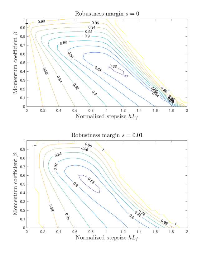
Figure 5: Plot of convergence rate $\rho$ of the Nesterov’s accelerated method as a function of stepsize $h$ and momentum parameter $\beta$, and for two values of the robustness parameter $s$. Higher values of $s$ increases the robustness of the algorithm at the expense of reduced convergence rate.

In Figure 5, we plot the contour plots of $\rho$ for $s=0$ and $s=0.01$, respectively. The condition number is fixed at $L_{f}/m_{f}=10$. We observe that when $s$ is nonzero, the parameters of the robust algorithm shift towards smaller stepsizes and higher momentum coefficients, leading to higher robustness and lower convergence rates.

7 Concluding remarks

In this paper, we have developed an LMI framework, built on the notion of Integral Quadratic Constraints from robust control theory and Lyapunov stability, to certify both exponential and subexponential convergence rates of first-order optimization algorithms. To this end, we proposed a class of time-varying Lyapunov functions that are suitable generating convergence rates in addition to proving stability. We showed that the developed LMI can often be solved in closed form. In particular, we applied the technique to the gradient method, the proximal gradient method, and their accelerated extensions to recover the known analytical upper bounds on their performance. Furthermore, we showed that numerical schemes can also be used to solve the LMI.

In this paper, we have only used pointwise IQCs to model nonlinearities. More complicated IQCs, such as“off-by-one” IQCs, have shown to be fruitful in improving numerical rate bounds in strongly convex settings [19]. One direction for future work would be to use these IQCs in tandem with the Lyapunov function used in this paper to further improve the numerical bounds in nonstrongly convex problems. Obtaining better worst-case bounds is useful in a variety of applications, such as Model Predictive Control (MPC). MPC is a sequential optimization-based control scheme, which is particularly useful for constrained and nonlinear control tasks. Implementation of MPC requires the solution of a constrained optimization problem in real time within the sampling period to a specific accuracy determined from stability considerations [26]. It is thus important to bound a priori, in a nonconservative manner, the number of iterations needed for a specified accuracy. Improving the numerical rate bounds will allow us to optimize this bound for every problem instance. More generally, having a nonconservative estimation of convergence rate allows us to compare different algorithms, which must be done by extensive simulations otherwise. We will pursue these applications in future work.

Appendix A Symbolic convergence rates for the gradient method

The LMI in (4.15) with $p=1$ along with the condition $a_{k+1}\geq a_{k}$ is equivalent to the inequalities

(A.1) $$a_{k+1}\geq a_{k},$$

(A.2) $$(\dfrac{L_{f}h^{2}}{2}-h)a_{k+1}+h^{2}-\dfrac{\sigma}{L_{f}}\leq 0,$$

(A.3) $$-\Big{(}\dfrac{a_{k+1}-a_{k}-2h+\sigma}{2}\Big{)}^{2}\geq 0.$$

The last inequality implies $a_{k+1}=a_{k}+2h-\sigma$. Assuming $a_{0}=0$ and solving for $a_{k}$, we obtain $a_{k}=(2h-\sigma)k$. Therefore, the fastest convergence rate corresponds to the smallest $\sigma$. By substituting $a_{k}$ in (A.1) and (A.2), we obtain

(A.4) $$2h-\sigma\geq 0,\quad(\dfrac{L_{f}h^{2}}{2}-h)(2h-\sigma)(k+1)+h^{2}-\dfrac{\sigma}{L_{f}}\leq 0.$$

Since the second inequality must hold for all $k\geq 0$, we must have that ${L_{f}h^{2}}/{2}-h\leq 0$ or equivalently, $0\leq h\leq 2/L_{f}$. Under this condition, it suffices to ensure the second inequality in (A.4) holds for $k=0$. This leads to

(A.5) $$\max(0,\dfrac{(L_{f}h)(L_{f}h-1)(2h)}{(L_{f}h)^{2}-2(L_{f}h)+2})\leq\sigma\leq 2h.$$

Therefore, the optimal (minimum) $\sigma$ is

(A.6) $$\sigma_{opt}=\begin{cases}0&\mbox{if }0\leq hL_{f}\leq 1\\ \dfrac{(L_{f}h)(L_{f}h-1)(2h)}{(L_{f}h)^{2}-2(L_{f}h)+2}&\mbox{if }1<hL_{f}\leq 2.\end{cases}$$

By substituting all the parameters in (3.4), we obtain

(A.7) $$f(x_{k})-f(x_{\star})\leq\dfrac{\|x_{0}-x_{\star}\|_{2}^{2}}{(2h-\sigma_{opt})k},$$

which is the same as (4.16). $\square$

Appendix B Proof of Proposition 5.1

Proof of part 1: Since $g$ is nondifferentiable and convex, it follows from the discussion in $\S$6.1.1 and $\S$6.1.2 that $\Pi_{g,h}$ is firmly non-expansive and is hence Lipschitz continuous with Lipschitz parameter equal to one. Further, it is well-known that the map $x\mapsto x-h\nabla f(x)$ is Lipschitz continuous with Lipschitz constant $\gamma_{f}=\max\{|1-hL_{f}|,|1-hm_{f}|\}$; see, for example, [4] for a proof. Therefore, the composition $\Pi_{g,h}(x-h\nabla f(x))$ is Lipschitz continuous with parameter $\gamma_{f}$. In other words, we can write

$$\|\Pi_{g,h}(x-h\nabla f(x))\!-\!\Pi_{g,h}(x_{\star}-h\nabla f(x_{\star}))\|_{2}^{2}\leq\gamma_{f}^{2}\|x-x_{\star}\|_{2}^{2}.$$

Making the substitution $\Pi_{g,h}(x-h\nabla f(x))=x-h\phi_{h}(x)$, completing the squares, and rearranging terms yield

$$\begin{bmatrix}x-x_{\star}\\ \phi_{h}(x)-\phi_{h}(x_{\star})\end{bmatrix}^{\top}\!\begin{bmatrix}\dfrac{1}{2h}(\gamma_{f}^{2}-1)I_{d}&\dfrac{1}{2}I_{d}\\ \dfrac{1}{2}I_{d}&-\dfrac{h}{2}I_{d}\end{bmatrix}\begin{bmatrix}x-x_{\star}\\ \phi_{h}(x)-\phi_{h}(x_{\star})\end{bmatrix}\geq 0.$$

Proof of part 2: First, note that the optimality condition of the proximal operator, defined in (5.3), is that

$$0\in\partial g(\Pi_{g,h}(w))+\dfrac{1}{h}(\Pi_{g,h}(w)-w),$$

or equivalently,

(B.1) $$0=T_{g}(\Pi_{g,h}(w))+\dfrac{1}{h}(\Pi_{g,h}(w)-w),\ T_{g}\in\partial g,$$

where $T_{g}(w)$ denotes a subgradient of $g$ at $w$. On the other hand, by the definition of the generalized gradient mapping in (5.4), we have that

(B.2) $$\Pi_{g,h}(y-h\nabla f(y))=y-h\phi_{h}(y).$$

Substituting (B.2) and $w=y-h\nabla f(y)$ in (B.1), we can equivalently write $\phi_{h}(y)$ as

(B.3) $$\phi_{h}(y)=\nabla f(y)+T_{g}(y-h\phi_{h}(y)).$$

Consider the points $x,y,z\in\mathrm{dom}\,f$. We can write

$$f(z)-f(y) \leq\nabla f(y)^{\top}(z\!-\!y)\!+\!\dfrac{L_{f}}{2}\|z\!-\!y\|_{2}^{2},$$

$$f(y)-f(x) \leq\nabla f(y)^{\top}(y\!-\!x)\!-\!\dfrac{m_{f}}{2}\|y\!-\!x\|_{2}^{2}.$$

In the first and second inequality, we have used Lipschitz continuity and strong convexity, respectively. Adding both sides yields

(B.4) $$f(z)\!-\!f(x)\!\leq\!\nabla f(y)^{\top}(z\!-\!x)+\dfrac{L_{f}}{2}\|z\!-\!y\|_{2}^{2}\!-\!\dfrac{m_{f}}{2}\|y\!-\!x\|_{2}^{2}.$$

Further, since $g$ is convex, we can write

(B.5) $$g(z)-g(x)\leq T_{g}(z)^{\top}(z-x),\quad T_{g}(z)\in\partial g(z),\quad x,z\in\mathrm{dom}\,g.$$

Adding both sides of (B.4) and (B.5) for all $x,z\in\mathrm{dom}\,f\cap\mathrm{dom}\,g,\ y\in\mathrm{dom}\,f$, and making the substitutions $z=y-h\phi_{h}(y)$ and (B.3) yields (5.6).

Proof of part 3: Suppose $\phi_{h}(y)=0$ for some $y\in\mathrm{dom}\,\phi_{h}$. It then follows from (B.3) that $0=\nabla f(y)+T_{g}(y)$, or equivalently, $0\in\nabla f(y)+\partial g(y)$. This implies that $y\in\mathcal{X}_{\star}$, according to (5.2). Conversely, suppose $y\in\mathcal{X}_{\star}$. We therefore have $\nabla f(y)=-T_{g}(y)$. Substituting this in (B.3) yields $\phi_{h}(y)=T_{g}(y-h\phi_{h}(y))-T_{g}(y)$. Since $T_{g}$ is monotone, we can write

$$0\leq(T_{g}(y-h\phi_{h}(y))-T_{g}(y))^{\top}(y-h\phi_{h}(y)-y)=-h\|\phi_{h}(y)\|_{2}^{2}\quad\mbox{for all }h.$$

Therefore, we must have that $\phi_{h}(y)=0$. The proof is now complete. $\square$

Appendix C Proof of Lemma 5.3

In order to bound $F(x_{k+1})-F(x_{k})$ and $F(x_{k+1})-F(x_{\star})$, we use the inequality

(C.1) $$F(y\!-\!h\phi_{h}(y))\!-\!F(x)\leq \phi_{h}(y)^{\top}(y\!-\!x)\!-\!\dfrac{m_{f}}{2}\|y\!-\!x\|_{2}^{2}+(\frac{1}{2}L_{f}h^{2}\!-\!h)\|\phi_{h}(y)\|_{2}^{2},$$

which we proved in Proposition 5.1. Specifically, we substitute $(x,y)=(x_{\star},y_{k})$ in (C.1) to get

$$F(x_{k+1})\!-\!F(x_{\star})\leq(u_{k}-u_{\star})^{\top}(y_{k}\!-\!y_{\star})\!+\!(\dfrac{L_{f}h^{2}}{2}\!-\!h)\|u_{k}-u_{\star}\|_{2}^{2}\!-\!\dfrac{m_{f}}{2}\|y_{k}\!-\!y_{\star}\|_{2}^{2}$$

$$=\begin{bmatrix}y_{k}-y_{\star}\\ u_{k}-u_{\star}\end{bmatrix}^{\top}\begin{bmatrix}-\frac{m_{f}}{2}&\frac{1}{2}\\ \frac{1}{2}&(\frac{1}{2}L_{f}h^{2}\!-\!h)\end{bmatrix}\begin{bmatrix}y_{k}-y_{\star}\\ u_{k}-u_{\star}\end{bmatrix}.$$

$$=\begin{bmatrix}\xi_{k}-\xi_{\star}\\ u_{k}-u_{\star}\end{bmatrix}^{\top}\begin{bmatrix}C_{k}&0\\ 0&I_{d}\end{bmatrix}^{\top}\begin{bmatrix}-\frac{m_{f}}{2}&\frac{1}{2}\\ \frac{1}{2}&(\frac{1}{2}L_{f}h^{2}\!-\!h)\end{bmatrix}\begin{bmatrix}C_{k}&0\\ 0&I_{d}\end{bmatrix}\begin{bmatrix}\xi_{k}-\xi_{\star}\\ u_{k}-u_{\star}\end{bmatrix}$$

$$=e_{k}^{\top}M_{k}^{2}e_{k}.$$

where we have used the identities $u_{\star}=\phi_{h}(y_{\star})=0$ and $y_{k}-y_{\star}=C_{k}(\xi_{k}-\xi_{\star})$. Similarly, in (C.1) we substitute $(x,y)=(x_{k},y_{k})$ to obtain

(C.2) $$F(x_{k+1})\!-\!F(x_{k})\leq(u_{k}-u_{\star})^{\top}(y_{k}-x_{k})\!+\!(\frac{1}{2}L_{f}h^{2}\!-\!h)\|u_{k}\!-\!u_{\star}\|_{2}^{2}\!-\!\dfrac{m_{f}}{2}\|y_{k}\!-\!x_{k}\|_{2}^{2}$$

$$=\begin{bmatrix}y_{k}-x_{k}\\ u_{k}-u_{\star}\end{bmatrix}^{\top}\begin{bmatrix}-\frac{m_{f}}{2}&\frac{1}{2}\\ \frac{1}{2}&(\frac{1}{2}L_{f}h^{2}\!-\!h)\end{bmatrix}\begin{bmatrix}y_{k}-x_{k}\\ u_{k}-u_{\star}\end{bmatrix}$$

$$=\begin{bmatrix}\xi_{k}-\xi_{\star}\\ u_{k}-u_{\star}\end{bmatrix}^{\top}\begin{bmatrix}C_{k}\!-\!E_{k}&0\\ 0&I_{d}\end{bmatrix}^{\top}\begin{bmatrix}-\frac{m_{f}}{2}&\frac{1}{2}\\ \frac{1}{2}&(\frac{1}{2}L_{f}h^{2}\!-\!h)\end{bmatrix}\begin{bmatrix}C_{k}\!-\!E_{k}&0\\ 0&I_{d}\end{bmatrix}\begin{bmatrix}\xi_{k}-\xi_{\star}\\ u_{k}-u_{\star}\end{bmatrix}$$

$$=e_{k}^{\top}M_{k}^{1}e_{k}.$$

where we have used $x_{\star}=y_{\star}$ and $y_{k}-x_{k}=(C_{k}-E_{k})(\xi_{k}-\xi_{\star})$ to obtain the second equality. Finally, by Proposition 5.1 $u_{k}=\phi_{h}(y_{k})$ satisfies the pointwise IQC defined by $(Q_{\phi_{h}},x_{\star},\phi_{h}(x_{\star}))$. Therefore, we can write

(C.3) $$e_{k}^{\top}M_{k}^{3}e_{k} =\begin{bmatrix}\xi_{k}-\xi_{\star}\\ u_{k}-u_{\star}\end{bmatrix}^{\top}\begin{bmatrix}C_{k}&0\\ 0&I_{d}\end{bmatrix}^{\top}Q_{\phi_{h}}\begin{bmatrix}C_{k}&0\\ 0&I_{d}\end{bmatrix}\begin{bmatrix}\xi_{k}-\xi_{\star}\\ u_{k}-u_{\star}\end{bmatrix}$$

$$=\begin{bmatrix}y_{k}-y_{\star}\\ u_{k}-u_{\star}\end{bmatrix}^{\top}Q_{\phi_{h}}\begin{bmatrix}y_{k}-y_{\star}\\ u_{k}-u_{\star}\end{bmatrix}$$

$$\geq 0,$$

where we have used the identity $y_{k}-y_{\star}=C_{k}(\xi_{k}-\xi_{\star})$ to obtain the second inequality. The proof is complete.

References

• [1] F. Alvarez, On the minimizing property of a second order dissipative system in hilbert spaces, SIAM Journal on Control and Optimization, 38 (2000), pp. 1102–1119.
• [2] H. Attouch, J. Peypouquet, and P. Redont, Fast convex optimization via inertial dynamics with hessian driven damping, Journal of Differential Equations, 261 (2016), pp. 5734–5783.
• [3] A. Beck and M. Teboulle, A fast iterative shrinkage-thresholding algorithm for linear inverse problems, SIAM journal on imaging sciences, 2 (2009), pp. 183–202.
• [4] D. P. Bertsekas, Convex optimization algorithms, Athena Scientific Belmont, 2015.
• [5] A. Cabot, H. Engler, and S. Gadat, On the long time behavior of second order differential equations with asymptotically small dissipation, Transactions of the American Mathematical Society, 361 (2009), pp. 5983–6017.
• [6] A. Cherukuri, E. Mallada, S. Low, and J. Cortes, The role of convexity on saddle-point dynamics: Lyapunov function and robustness, arXiv preprint arXiv:1608.08586, (2016).
• [7] P. L. Combettes and J.-C. Pesquet, Proximal splitting methods in signal processing, in Fixed-point algorithms for inverse problems in science and engineering, Springer, 2011, pp. 185–212.
• [8] S. Cyrus, B. Hu, B. Van Scoy, and L. Lessard, A robust accelerated optimization algorithm for strongly convex functions, arXiv preprint arXiv:1710.04753, (2017).
• [9] O. Devolder, F. Glineur, and Y. Nesterov, First-order methods of smooth convex optimization with inexact oracle, Mathematical Programming, 146 (2014), pp. 37–75.
• [10] Y. Drori and M. Teboulle, Performance of first-order methods for smooth convex minimization: a novel approach, Mathematical Programming, 145 (2014), pp. 451–482.
• [11] M. Fazlyab, A. Ribeiro, M. Morari, and V. M. Preciado, A dynamical systems perspective to convergence rate analysis of proximal algorithms, in 2017 55th Annual Allerton Conference on Communication, Control, and Computing (Allerton), Oct 2017, pp. 354–360, https://doi.org/10.1109/ALLERTON.2017.8262759.
• [12] D. Feijer and F. Paganini, Stability of primal–dual gradient dynamics and applications to network optimization, Automatica, 46 (2010), pp. 1974–1981.
• [13] M. Hardt, T. Ma, and B. Recht, Gradient descent learns linear dynamical systems, arXiv preprint arXiv:1609.05191, (2016).
• [14] E. Hazan, K. Levy, and S. Shalev-Shwartz, Beyond convexity: Stochastic quasi-convex optimization, in Advances in Neural Information Processing Systems, 2015, pp. 1594–1602.
• [15] B. Hu and L. Lessard, Control interpretations for first-order optimization methods, in American Control Conference, May 2017, pp. 3114–3119, https://doi.org/10.23919/ACC.2017.7963426.
• [16] B. Hu and L. Lessard, Dissipativity theory for Nesterov’s accelerated method, in International Conference on Machine Learning, Aug. 2017, pp. 1549–1557.
• [17] H. Karimi, J. Nutini, and M. Schmidt, Linear convergence of gradient and proximal-gradient methods under the polyak-Łojasiewicz condition, in Joint European Conference on Machine Learning and Knowledge Discovery in Databases, Springer, 2016, pp. 795–811.
• [18] D. Kim and J. A. Fessler, Optimized first-order methods for smooth convex minimization, Mathematical programming, 159 (2016), pp. 81–107.
• [19] L. Lessard, B. Recht, and A. Packard, Analysis and design of optimization algorithms via integral quadratic constraints, SIAM Journal on Optimization, 26 (2016), pp. 57–95.
• [20] A. Megretski and A. Rantzer, System analysis via integral quadratic constraints, IEEE Transactions on Automatic Control, 42 (1997), pp. 819–830.
• [21] I. Necoara, Y. Nesterov, and F. Glineur, Linear convergence of first order methods for non-strongly convex optimization, arXiv preprint arXiv:1504.06298, (2015).
• [22] Y. Nesterov, A method of solving a convex programming problem with convergence rate o (1/k2), in Soviet Mathematics Doklady, vol. 27, 1983, pp. 372–376.
• [23] Y. Nesterov, Introductory lectures on convex optimization: A basic course, 2013.
• [24] R. Nishihara, L. Lessard, B. Recht, A. Packard, and M. I. Jordan, A general analysis of the convergence of ADMM, arXiv preprint arXiv:1502.02009, (2015).
• [25] B. Polyak, Some methods of speeding up the convergence of iteration methods, USSR Computational Mathematics and Mathematical Physics, 4 (1964), pp. 1 – 17, https://doi.org/https://doi.org/10.1016/0041-5553(64)90137-5, http://www.sciencedirect.com/science/article/pii/0041555364901375.
• [26] S. Richter, C. N. Jones, and M. Morari, Computational complexity certification for real-time mpc with input constraints based on the fast gradient method, IEEE Transactions on Automatic Control, 57 (2012), pp. 1391–1403.
• [27] W. Su, S. Boyd, and E. J. Candes, A differential equation for modeling nesterov’s accelerated gradient method: theory and insights, Journal of Machine Learning Research, 17 (2016), pp. 1–43.
• [28] A. B. Taylor, J. M. Hendrickx, and F. Glineur, Exact worst-case convergence rates of the proximal gradient method for composite convex minimization, arXiv preprint arXiv:1705.04398, (2017).
• [29] A. B. Taylor, J. M. Hendrickx, and F. Glineur, Smooth strongly convex interpolation and exact worst-case performance of first-order methods, Mathematical Programming, 161 (2017), pp. 307–345.
• [30] J. Wang and N. Elia, Control approach to distributed optimization, in Communication, Control, and Computing (Allerton), 2010 48th Annual Allerton Conference on, IEEE, 2010, pp. 557–561.
• [31] J. Wang and N. Elia, A control perspective for centralized and distributed convex optimization, in 2011 50th IEEE Conference on Decision and Control and European Control Conference, IEEE, 2011, pp. 3800–3805.
• [32] A. Wibisono, A. C. Wilson, and M. I. Jordan, A variational perspective on accelerated methods in optimization, Proceedings of the National Academy of Sciences, (2016), p. 201614734.
• [33] A. C. Wilson, B. Recht, and M. I. Jordan, A lyapunov analysis of momentum methods in optimization, arXiv preprint arXiv:1611.02635, (2016).
• [34] V. Yakubovich, Frequency conditions for the absolute stability of control systems with several nonlinear or linear nonstationary blocks, Avtomatika i telemekhanika, 6 (1967), pp. 5–30.