Accelerating equilibrium isotope effect calculations: I. Stochastic thermodynamic integration with respect to mass

Abstract

Accurate path integral Monte Carlo or molecular dynamics calculations of isotope effects have until recently been expensive because of the necessity to reduce three types of errors present in such calculations: statistical errors due to sampling, path integral discretization errors, and thermodynamic integration errors. While the statistical errors can be reduced with virial estimators and path integral discretization errors with high-order factorization of the Boltzmann operator, here we propose a method for accelerating isotope effect calculations by eliminating the integration error. We show that the integration error can be removed entirely by changing particle masses stochastically during the calculation and by using a piecewise linear umbrella biasing potential. Moreover, we demonstrate numerically that this approach does not increase the statistical error. The resulting acceleration of isotope effect calculations is demonstrated on a model harmonic system and on deuterated species of methane.

I Introduction

The equilibrium (or thermodynamic) isotope effectWolfsberg et al. (2010) is defined as the effect of isotopic substitution on the equilibrium constant of a chemical reaction. More precisely, the equilibrium isotope effect is the ratio of equilibrium constants,

$$\mathrm{EIE}:=\frac{K^{(B)}}{K^{(A)}},$$ (1)

where $A$ and $B$ are two isotopologues of the reactant. Since an equilibrium constant can be evaluated as the ratio of the product and reactant partition functions ($K=Q_{\text{prod}}/Q_{\text{react}}$), every equilibrium isotope effect can be written as a product of several “elementary” isotope effects (IEs),

$$\mathrm{IE}=\frac{Q^{(B)}}{Q^{(A)}},$$ (2)

given by the ratio of partition functions corresponding to different isotopologues (of either the reactant or product).

This quantity is closely related to the important notion of isotope fractionation,Urey (1947); Wolfsberg et al. (2010); McKenzie, Athokpam, and Ramesh (2015) which describes the distribution of isotopes in different substances or different phases and can be expressed in terms of such elementary isotope effects (2) if kinetic factors can be neglected. Below, we will therefore focus on finding these elementary ratios of partition functions and call them “isotope effects” for short.

The isotope effect is extremely useful in uncovering the influence of nuclear quantum effects on molecular properties,Janak and Parkin (2003); Wolfsberg et al. (2010); McKenzie, Athokpam, and Ramesh (2015) hence many approaches have been developed to calculate it. The simplest and most common approach, usually referred to as the “harmonic approximation” or “Urey model”, assumes (i) separability of rotations and vibrations, (ii) rigid rotor approximation for the rotations, and (iii) harmonic oscillator approximation for the vibrations.Urey (1947); Wolfsberg et al. (2010); Webb and Miller III (2014) Although there exist various corrections that incorporate the leading effects of rovibrational coupling, nonrigidity of the rotor, or anharmonicity of the vibrations,Richet, Bottinga, and Javoy (1977); Barone (2004); Liu, Tossell, and Liu (2010) this perturbative approach is not always sufficient; indeed, there are examples of systems in which these corrections can even yield worse results than the Urey model.Webb and Miller III (2014)

We therefore employ a more rigorous method that avoids these approximations altogether and treats the potential energy surface, rotations, and rovibrational coupling exactly. To show the benefit of this rigorous approach, in Figure 1 we plot the relative error of $\mathrm{CD}_{4}/\mathrm{CH}_{4}$ IE calculated with the harmonic approximation. In this example, the harmonic approximation works rather well at higher temperatures, where the IE is small, but its error reaches as much as $60\%$ at the low temperature of $200$ K, where the IE becomes very large.

The potentially large errors of the harmonic approximation are eliminated in the Feynman path integral formalism,Feynman and Hibbs (1965); Chandler and Wolynes (1981); Ceperley (1995) in which the quantum partition function is transformed to a classical partition function of the so-called ring polymer; it is then possible to compute the isotope effect via the thermodynamic integrationKirkwood (1935); Frenkel and Smit (2002); Tuckerman (2010) with respect to mass,Vaníček et al. (2005); Vaníček and Miller (2007); Zimmermann and Vaníček (2009, 2010); Pérez and von Lilienfeld (2011) which treats the isotope masses as continuous variables and allows using standard path integral molecular dynamics or Monte Carlo techniques. The main drawback of this approach is that the “mass integral” is evaluated by discretizing the mass, which introduces an integration error. Although several elegant tricks reduce this integration error significantly,Ceriotti and Markland (2013); Maršálek et al. (2014) it can never be removed completely if the integral is evaluated deterministically.

Figure 1: Temperature dependence of the relative error of the $\mathrm{CD_{4}/CH_{4}}$ isotope effect (IE) obtained with the harmonic approximation. The result of stochastic thermodynamic integration (STI, see Subsec. III.3) serves as a reference; the relative error is defined as IE(harmonic)/IE(STI) - 1.

Here we propose a way to bypass this issue by augmenting the configuration space of the Monte Carlo simulation with an extra dimension $\lambda$ corresponding to the mass and including this dimension in the stochastic integration. The main idea is quite similar to that employed in the more general $\lambda$-dynamics methodLiu and Berne (1993); Kong and Brooks III (1996); Guo, Brooks III, and Kong (1998); Bitetti-Putzer, Yang, and Karplus (2003); Pérez and von Lilienfeld (2011) used in molecular dynamics or Monte Carlo simulations, but we introduce a Monte Carlo procedure which is applicable for the specific case of the change of mass and enables a faster exploration of the $\lambda$ dimension. We find that the proposed stochastic approach reduces the integration error of the IE drastically without increasing the statistical error. Remarkably, we also show that the integration error can be reduced to zero exactly by using a piecewise linear umbrella biasing potential; the only remaining error of the calculated IE is due to statistical factors.

To assess the numerical performance of the proposed methodology, we apply it to the isotope effects in an eight-dimensional harmonic model and in a full-dimensional $\mathrm{CH}_{4}$ molecule. Methane was chosen because the $\mathrm{CH_{4}+D_{2}}$ exchange is an important benchmark reaction for studying catalysis of hydrogen exchange over metalsOsawa et al. (2010) and metal oxides,Hargreaves et al. (2002) and because the polydeuterated species $\mathrm{CH_{4-x}D_{x}}$ are formed in abundance during the catalyzed reaction.

II Theory

II.1 Path integral representation of the partition function

Let us consider a molecular system consisting of $N$ atoms with masses $m_{i}$ ($i=1,\ldots,N$) moving in $D$ spatial dimensions (typically, $D=3$, of course). To apply the path integral formalism to the isotope effect (2), one first needs a path integral representation of the partition function $Q:=\operatorname{Tr}\exp(-\beta\hat{H})$.

This representation is obtained by factoring the Boltzmann operator $\exp(-\beta\hat{H})=[\exp(-\beta\hat{H}/P)]^{P}$ into $P$ so-called imaginary time slices, inserting a coordinate resolution of identity between each two adjacent factors, using a high-temperature approximation for each factor $\exp(-\beta\hat{H}/P)$, and taking a limit $P\rightarrow\infty$, in which the high-temperature approximation becomes exact. The well-knownFeynman and Hibbs (1965); Chandler and Wolynes (1981) final result

$$Q=\lim_{P\rightarrow\infty}Q_{P}$$ (3)

expresses the partition function as the $P\rightarrow\infty$ limit of the discretized path integral representation

$$Q_{P}=\int d\mathbf{r}\rho(\mathbf{r})\text{,}$$ (4)

where $\mathbf{r}$ is a vector containing all $PND$ coordinates of all atoms in all slices of the extended configuration space; more precisely, $\mathbf{r}:=\left(\mathbf{r}^{(1)},\ldots,\mathbf{r}^{(P)}\right)$, where $\mathbf{r}^{\left(s\right)}$, $s=1,\ldots,P$, is a vector containing all $ND$ coordinates of all atoms in slice $s$. In general, a subscript $P$ on a quantity $A$ will denote a discretized path integral representation of $A$ using $P$ imaginary time slices. The statistical weight $\rho(\mathbf{r})$ of each path integral configuration is given by

$$\rho(\mathbf{r})=C\exp\left[-\beta\Phi(\mathbf{r})\right]\text{,}$$ (5)

with the prefactor

$$C=\left(\frac{P}{2\beta\hbar^{2}\pi}\right)^{NDP/2}\left(\prod_{i=1}^{N}m_{i}\right)^{DP/2},$$ (6)

and with an effective potential energy of the classical ring polymer given by

$$\Phi(\mathbf{r})=\frac{P}{2\beta^{2}\hbar^{2}}\sum_{i=1}^{N}m_{i}\sum_{s=1}^{P}|\mathrm{r}_{i}^{(s)}-\mathrm{r}_{i}^{(s-1)}|^{2}+\frac{1}{P}\sum_{s=1}^{P}V(\mathbf{r}^{(s)})\text{,}$$ (7)

where $\mathrm{r}_{i}^{(s)}$ denotes the component of $\mathbf{r}^{(s)}$ corresponding to atom $i$ (i.e. $\mathrm{r}_{i}^{(s)}$ is a vector containing the $D$ coordinates of the $i$th atom), and $V$ is the potential energy of the original system. Since the factorization of the Boltzmann operator is an example of the Lie-Trotter factorization, the number $P$ is also referred to as the Trotter number. Because the path employed to represent the partition function is a closed path, we define $\mathbf{r}^{(0)}:=\mathbf{r}^{(P)}$; this convention was already used in Eq. (7) for $s=1$.

Note that $Q_{P}$ is a classical partition function of the ring polymer, i.e., a system in the extended configuration space with $NDP$ classical degrees of freedom and defined by the effective potential $\Phi(\mathbf{r})$. For $P=1$ the path integral expression (4) for the quantum partition function reduces to the classical one.

II.2 Thermodynamic integration with respect to mass

Our ultimate goal is evaluating the isotope effect (2), i.e., a ratio of partition functions. Although it is possible to evaluate partition functions $Q_{P}^{(A)}$ and $Q_{P}^{(B)}$ themselves with a Monte Carlo procedure,Lynch, Mielke, and Truhlar (2005) it is more convenient to calculate the ratio $Q_{P}^{(B)}/Q_{P}^{(A)}$ directly. We now review the most common of such direct approaches, based on thermodynamic integrationKirkwood (1935) with respect to mass.Vaníček et al. (2005)

In this method, it is assumed that the isotope change is continuous and parametrized by a dimensionless parameter $\lambda\in[0,1]$, where $\lambda=0$ corresponds to isotopologue $A$ and $\lambda=1$ to isotopologue $B$. This allows, e.g., the description of the isotope effect when several atoms in a molecule are replaced by their isotopes simultaneously. Therefore we define, for each atom $i$, a continuous function $m_{i}(\lambda)$ of $\lambda$ such that

$$m_{i}(0) =m_{i}^{(A)},$$ (8)

$$m_{i}(1) =m_{i}^{(B)}.$$ (9)

The simplest possible choice for the interpolating function is the linear interpolation

$$m_{i}(\lambda)=\left(1-\lambda\right)m_{i}^{(A)}+\lambda m_{i}^{(B)},$$ (10)

used in Refs. Vaníček et al., 2005; Vaníček and Miller, 2007; Zimmermann and Vaníček, 2009, but Ceriotti and MarklandCeriotti and Markland (2013) showed that a faster convergence, especially in the deep quantum regime, is often achieved by interpolating the inverse square roots of the masses,

$$\frac{1}{\sqrt{m_{i}(\lambda)}}=\left(1-\lambda\right)\frac{1}{\sqrt{m_{i}^{(A)}}}+\lambda\frac{1}{\sqrt{m_{i}^{(B)}}},$$ (11)

which is therefore the interpolation used in the numerical examples below, unless explicitly mentioned otherwise.

Letting $Q(\lambda)$ denote the partition function of a fictitious system with interpolated masses $m_{i}(\lambda)$, we can express the isotope effect (2) as

$$\frac{Q^{(B)}}{Q^{(A)}} =\exp\left[\int_{0}^{1}\frac{d\ln Q(\lambda)}{d\lambda}d\lambda\right]$$ (12)

$$=\exp\left[-\beta\int_{0}^{1}\frac{dF(\lambda)}{d\lambda}d\lambda\right],$$ (13)

where $F(\lambda)$ is the free energy corresponding to the isotope change and the integral in the exponent motivated the name “thermodynamic integration.” While it is difficult to evaluate either $Q_{P}^{(A)}$ or $Q_{P}^{(B)}$ with a path integral Monte Carlo method, the logarithmic derivative $d\ln Q_{P}(\lambda)/d\lambda=\left[dQ_{P}(\lambda)/d\lambda\right]/Q_{P}(\lambda)=-\beta dF_{P}(\lambda)/d\lambda$ is a normalized quantity, i.e., a thermodynamic average proportional to the free energy derivative with respect to $\lambda$, and therefore can be computed easily with the Metropolis algorithm with sampling weight $\rho^{(\lambda)}(\mathbf{r})$ corresponding to the fictitious system with masses $m_{i}(\lambda)$:

$$dF_{P}(\lambda)/d\lambda=\left\langle\left[dF(\lambda)/d\lambda\right]_{\text{est}}\right\rangle^{(\lambda)}.$$

Here we have introduced general notation

$$\left\langle A_{\text{est}}\right\rangle^{(\lambda)}:=\frac{\int d\mathbf{r}A_{\text{est}}(\mathbf{r})\rho^{(\lambda)}(\mathbf{r})}{\int d\mathbf{r}\rho^{(\lambda)}(\mathbf{r})}$$

for a thermodynamic path integral average of an observable $A$, given by averaging the estimator $A_{\text{est}}$ over an ensemble with weight $\rho^{(\lambda)}(\mathbf{r})$. The so-called thermodynamic estimator $\left[dF(\lambda)/d\lambda\right]_{\text{th}}$ for $dF_{P}(\lambda)/d\lambda$ is derived simply by differentiating Eq. (4),

$$\left[dF(\lambda)/d\lambda\right]_{\text{th}}=-\frac{1}{\beta}\sum_{i=1}^{N}\frac{dm_{i}}{d\lambda}\left[\frac{DP}{2m_{i}}-\frac{P}{2\beta\hbar^{2}}\sum_{s=1}^{P}|\mathrm{r}_{i}^{(s)}-\mathrm{r}_{i}^{(s-1)}|^{2}\right].$$ (14)

However, since it is a difference of two terms proportional to $P$, this estimator has a statistical error that grows with the Trotter number $P$, further increasing the computational cost. This drawback motivated the introductionVaníček and Miller (2007) of the centroid virial estimator $\left[dF(\lambda)/d\lambda\right]_{\text{cv}}$ whose statistical error is independent of $P$, a property mirroring the property of an analogous centroid virial estimator for kinetic energy.Predescu and Doll (2002); Yamamoto (2005) The centroid virial estimator, derived in Appendix A, is given by

$$\left[dF(\lambda)/d\lambda\right]_{\text{cv}}=-\sum_{i=1}^{N}\frac{1}{2m_{i}}\frac{dm_{i}}{d\lambda}\left\{\frac{D}{\beta}+\frac{1}{P}\sum_{s=1}^{P}\left[(\mathrm{r}_{i}^{(s)}-\mathrm{r}_{i}^{(C)})\cdot\nabla_{i}V(\mathbf{r}^{(s)})\right]\right\},$$ (15)

where

$$\mathbf{r}^{(C)}:=\frac{1}{P}\sum_{s=1}^{P}\mathbf{r}^{(s)}$$ (16)

is the centroid coordinate of the polymer ring. All our numerical examples use the centroid virial estimators, unless explicitly mentioned otherwise.

To summarize, using thermodynamic integration, the isotope effect (2) is evaluated as

$$\frac{Q_{P}^{(B)}}{Q_{P}^{(A)}}=\exp\left\{-\beta\int_{0}^{1}\left\langle\left[dF(\lambda)/d\lambda\right]_{\text{cv}}\right\rangle^{(\lambda)}d\lambda\right\}.$$ (17)

The calculation of the isotope effect requires running simulations at different values of $\lambda$ and then numerically evaluating the integral in Eq. (17) using, for example, the trapezoidal, midpoint, or Simpson rule.

II.3 Stochastic thermodynamic integration with respect to mass

It is evident that the method of thermodynamic integration introduces an integration error, and therefore several approaches have been proposed to decrease it: While Ceriotti and MarklandCeriotti and Markland (2013) optimized the interpolation functions $m_{i}(\lambda)$ in order to make $dF_{P}(\lambda)/d\lambda$ as flat as possible over the integration interval, and thus obtained Eq. (11), Maršálek and TuckermanMaršálek et al. (2014) introduced higher-order derivatives of $Q(\lambda)$ with respect to $\lambda$. Both modifications decrease the integration error, but do not eliminate it completely. In this subsection we show that including the $\lambda$ variable as an additional dimension in the Monte Carlo simulation allows to make the integration error exactly zero if an appropriate sampling procedure is used.

To illustrate why it makes sense to evaluate the $\lambda$ integral stochastically, let us consider a “standard” thermodynamic integration protocol from the previous subsection, where the integral in Eq. (12) is evaluated deterministically by discretizing the $\lambda$ interval $\left[0,1\right]$ into $J$ subintervals of the form $I_{j}=[\lambda_{j-1},\lambda_{j}]$, typically with $\lambda_{j}=j/J$ ($j=0,\dots,J$). For example, employing the midpoint rule for the integral, one would run a separate Monte Carlo simulation for each $\bar{\lambda}_{j}:=\left(\lambda_{j-1}+\lambda_{j}\right)/2=\left(j-1/2\right)/J\in I_{j}$ ($j=1,\dots,J$) in order to calculate $dF(\lambda)/d\lambda|_{\lambda=\bar{\lambda}_{j}}$. Suppose we increase $J$ while keeping the length of each simulation inversely proportional to $J$. Then the total number of Monte Carlo steps used will remain constant, the integration error will decrease, and the statistical error of the evaluated isotope effect will be close to a limiting value as long as each individual simulation is statistically converged. Unfortunately, for a fixed overall cost one cannot use arbitrarily large values of $J$, since that would render the individual simulations so short that their ergodicity would no longer be guaranteed. If ergodicity of an individual simulation requires at least $M_{\text{erg}}$ Monte Carlo steps, the cost of the calculation will grow as $\mathcal{O}(J\,M_{\text{erg}})$, making the limit $J\rightarrow\infty$ unattainable in practice.

If, instead of $J$ separate simulations for each $\bar{\lambda}_{j}$, one performs a single Monte Carlo simulation in a configuration space with an extra dimension corresponding to $\lambda$, the average of estimator $\left[dF(\lambda)/d\lambda\right]_{\text{cv}}$ over each subinterval $I_{j}$ will give an estimate for $dF(\lambda)/d\lambda|_{\lambda=\bar{\lambda}_{j}}$, and one can use much higher values of $J$ (and therefore obtain smaller integration errors) without sacrificing ergodicity of the simulation. This trick bears some resemblance to umbrella integrationKästner and Thiel (2005); Kästner (2009, 2012) and adaptive biasing forceDarve and Pohorille (2001); Darve, Rodrígues-Gómez, and Pohorille (2008); Comer et al. (2015) approaches used to find the dependence of free energy on a reaction coordinate, but here the role of reaction coordinate is taken by isotope masses. As in umbrella integration, decreasing the widths of the $\lambda$ intervals $I_{j}$ decreases the integration error without affecting the statistical error of the computed isotope effect.

Running a Monte Carlo simulation in a configuration space augmented by $\lambda$ requires, first of all, a correct sampling weight, $\rho^{(\lambda)}(\mathbf{r})$, which is nothing but $\rho(\mathbf{r})$ with masses $m_{i}(\lambda)$ evaluated at a given value $\lambda$. The second most important thing is a corresponding Monte Carlo trial move together with an acceptance rule. The simplest possible trial move with respect to $\lambda$ changes the initial $\lambda^{\prime}$ to any other $\lambda^{\prime\prime}\in[0,1]$ with equal probability, and keeps the Cartesian coordinates $\mathbf{r}$ of the ring polymer fixed. The resulting ratio of probability densities corresponding to $\lambda^{\prime\prime}$ and $\lambda^{\prime}$ is

$$\frac{\rho^{(\lambda^{\prime\prime})}(\mathbf{r})}{\rho^{(\lambda^{\prime})}(\mathbf{r})}=\left[\prod_{i=1}^{N}\frac{m_{i}(\lambda^{\prime\prime})}{m_{i}(\lambda^{\prime})}\right]^{PD/2}\exp\left\{\frac{P}{2\beta\hbar^{2}}\sum_{i=1}^{N}[m_{i}(\lambda^{\prime})-m_{i}(\lambda^{\prime\prime})]\sum_{s=1}^{P}|\mathrm{r}_{i}^{(s)}-\mathrm{r}_{i}^{(s-1)}|^{2}\right\},$$ (18)

which, as a function of $\lambda^{\prime\prime}$, has a maximum that unfortunately becomes sharper with larger $P$. A simple way to keep acceptance probability high even for large values of $P$ is to generate trial $\lambda^{\prime\prime}$ such that $\left|\lambda^{\prime\prime}-\lambda^{\prime}\right|\leq\Delta\lambda_{{\mathrm{max}}}$. The following Monte Carlo procedure satisfies this condition and also preserves the acceptance ratio given by Eq. (18):

Simple $\lambda$-move:

1. Trial move:

   $$\lambda^{\prime} \mapsto\lambda^{\prime\prime}=\lambda^{\prime}+\Delta\lambda\text{, where}$$ (19)

   $$\Delta\lambda\in[-\Delta\lambda_{\mathrm{max}},\Delta\lambda_{\mathrm{max}}]\text{ and distributed uniformly.}$$ (20)

2. Readjust the trial move to satisfy $\lambda^{\prime\prime}\in[0,1]$:

   $$\text{if }(\lambda^{\prime\prime}<0)\text{ then } \lambda^{\prime\prime}\mapsto-\lambda^{\prime\prime},$$ (21)

   $$\text{if }(\lambda^{\prime\prime}>1)\text{ then } \lambda^{\prime\prime}\mapsto 2-\lambda^{\prime\prime}.$$ (22)

3. Accept the final trial move with a probability

   $$\mathrm{min}\left(1,\left[\prod_{i=1}^{N}\frac{m_{i}(\lambda^{\prime\prime})}{m_{i}(\lambda^{\prime})}\right]^{PD/2}\exp\left\{\frac{P}{2\beta\hbar^{2}}\sum_{i=1}^{N}[m_{i}(\lambda^{\prime})-m_{i}(\lambda^{\prime\prime})]\sum_{s=1}^{P}|\mathrm{r}_{i}^{(s)}-\mathrm{r}_{i}^{(s-1)}|^{2}\right\}\right).$$ (23)

The procedure defined by Eqs. (19)-(23) is almost free in terms of computational time, but at very large values of $P$, even with the restriction (20), it becomes ineffective at sampling $\lambda$ values far from the maximum of the probability ratio (18). This problem can be bypassed if the trial move with respect to $\lambda$ preserves the mass-scaled normal modes of the ring polymer instead of the Cartesian coordinates, resulting in the following Monte Carlo procedure derived in Appendix A:

Mass-scaled $\lambda$-move:

1. Trial move:

   $$\lambda^{\prime} \mapsto\lambda^{\prime\prime}\in\left[0,1\right]\text{ and distributed uniformly},$$ (24)

   $$\mathbf{r} \mapsto\mathbf{r}_{\lambda^{\prime},\lambda^{\prime\prime}},$$ (25)

   where

   $$\mathrm{r}_{\lambda^{\prime},\lambda^{\prime\prime},i}^{(s)}:=\mathrm{r}_{i}^{(C)}+\sqrt{\frac{m_{i}(\lambda^{\prime})}{m_{i}(\lambda^{\prime\prime})}}(\mathrm{r}_{i}^{(s)}-\mathrm{r}_{i}^{(C)})\text{.}$$ (26)

2. Accept the trial move with a probability

   $$\mathrm{min}\left(1,\left[\prod_{i=1}^{N}\frac{m_{i}(\lambda^{\prime\prime})}{m_{i}(\lambda^{\prime})}\right]^{D/2}\exp\left\{\frac{\beta}{P}\sum_{s=1}^{P}[V(\mathbf{r}^{(s)})-V(\mathbf{r}_{\lambda^{\prime},\lambda^{\prime\prime}}^{(s)})]\right\}\right).$$ (27)

When discussing Monte Carlo moves with respect to $\lambda$, we shall refer the procedure defined by Eqs. (19)-(23) as the “simple $\lambda$-move”, and to that of Eqs. (24)-(27) as the “mass-scaled $\lambda$-move”. If the centroid probability distribution starts to vary too much over $\lambda\in[0,1]$, the acceptance probability for the mass-scaled $\lambda$-move can become too low; this is solved easily by restricting the trial $\lambda^{\prime\prime}$ value to a smaller interval $[\lambda^{\prime}-\Delta\lambda_{\mathrm{max}},\lambda^{\prime}+\Delta\lambda_{\max}]$ using the procedure of Eqs. (19)-(22). [Yet, for all systems considered in this work, Eqs. (24)-(27) led to sufficiently high acceptance probability without this modification.] The main advantage of the mass-scaled $\lambda$-move is that its acceptance probability does not depend on $P$. Its disadvantage is its requirement of $P$ evaluations of $V$, which makes it much more expensive than the simple $\lambda$-move. Nonetheless, as will be demonstrated in Sec. III, an occasional use of mass-scaled $\lambda$-moves can, in fact, accelerate convergence with respect to $\lambda$.

The Monte Carlo procedure has one last shortcoming: Since the probability of finding the system with $\lambda=\lambda^{\prime}$ is proportional to $Q(\lambda^{\prime})$, for very large isotope effects (the largest isotope effect computed in this work was $\sim 10^{8}$) most of the samples would be taken in the region close to $\lambda=0$, which would introduce a huge statistical error. This problem can be solved by adding a biasing umbrella potential $U_{b}(\lambda)$, resulting in a biased probability density

$$\rho_{b}^{(\lambda)}(\mathbf{r})=\rho^{(\lambda)}(\mathbf{r})\exp[-\beta U_{b}(\lambda)].$$ (28)

In the case of a free particle, all trial moves defined by Eqs. (24)-(26) will be accepted provided that the optimal biasing potential

$$U_{b,\mathrm{free}}(\lambda)=\frac{D}{2\beta}\sum_{i=1}^{N}\ln[m_{i}(\lambda)/m_{i}(0)]$$ (29)

is chosen; in other words, if $V\equiv 0$, then including $U_{b,\mathrm{free}}(\lambda)$ in the acceptance probability (27) will make it unity.

With this final modification in place, the proposed method can be summarized as running a Monte Carlo simulation in the augmented configuration space and then evaluating the isotope effect with the formula

$$\frac{Q_{P}^{(B)}}{Q_{P}^{(A)}}=\lim_{J\rightarrow\infty}\exp\left[-\frac{\beta}{J}\sum_{j=1}^{J}\left\langle\left[dF(\lambda)/d\lambda\right]_{\text{cv}}\right\rangle^{I_{j}}\right],$$ (30)

where $\langle\cdots\rangle^{I_{j}}$ is an average over all $\lambda\in I_{j}$. The integration error associated with having a finite number $J$ of $\lambda$ intervals depends strongly on the choice of the umbrella potential $U_{b}(\lambda)$. As we prove in Appendix B, this error is exactly zero for a piecewise linear umbrella potential satisfying

$$\frac{dU_{b}(\lambda)}{d\lambda}=-\langle[dF(\lambda)/d\lambda]_{\mathrm{cv}}\rangle^{I_{j}}\text{ for all $\lambda\in I_{j}$}.$$ (31)

It is also clear that the resulting $U_{b}(\lambda)$ will follow fairly closely the ideal biasing potential $\beta^{-1}\ln Q(\lambda)$, and therefore the estimator samples will be distributed more or less equally among different intervals $I_{j}$, which, in turn, will minimize the statistical error of Eq. (30).

It is obvious that in general systems, $U_{b}(\lambda)$ from Eq. (31) cannot be known a priori. As this is typical for biased simulations, numerous methods, including adaptive umbrella sampling,Mezei (1987); Hooft, van Eijck, and Kroon (1992); Bartels and Karplus (1997) metadynamics,Micheletti, Laio, and Parrinello (2004); Laio et al. (2005) and adaptive biasing force method,Darve and Pohorille (2001); Darve, Rodrígues-Gómez, and Pohorille (2008) have been introduced to solve this problem. In our calculations, the biasing potential $U_{b}(\lambda)$ was obtained from a short simulation employing the adaptive biasing force method. The resulting $U_{b}(\lambda)$ was then used in a longer simulation in which the isotope effect itself was evaluated.

III Numerical examples

In this section the proposed stochastic procedure for evaluating isotope effects is tested on a model harmonic system and on deuteration of methane. The results of the new approach are compared with results of the usual thermodynamic integration and with the analytical result for the harmonic system. From now on, for brevity we will refer to the traditional thermodynamic integration with respect to mass (Subsec. II.2) simply as “thermodynamic integration” (TI), and to the thermodynamic integration with stochastic change of mass (Subsec. II.3) as “stochastic thermodynamic integration” (STI). In all cases, we compare STI with TI both for the linear [Eq. (10)] and the more efficient [Eq. (11)] interpolation of mass.

III.1 Computational details

As mentioned in Sec. II, the $\lambda$ interval $\left[0,1\right]$ was divided into $J$ subintervals $I_{j}=[\lambda_{j-1},\lambda_{j}]$ $\left(j=1,\ldots,J\right)$ with $\lambda_{j}=j/J$ ($j=0,\dots,J$). The TI used, in addition, a reference point $\bar{\lambda}_{j}$ from each interval, which was always taken to be the midpoint $\overline{\lambda}_{j}=(j-1/2)/J\in I_{j}$. This midpoint was used for evaluating the thermodynamic integral with the midpoint rule as

$$\int_{0}^{1}\frac{d\ln Q(\lambda)}{d\lambda}d\lambda=\frac{1}{J}\sum_{j=1}^{J}\left.\frac{d\ln Q(\lambda)}{d\lambda}\right|_{\lambda=\bar{\lambda}_{j}}+\mathcal{O}\left(J^{-2}\right).$$ (32)

(Assuming that each logarithmic derivative is obtained with the same statistical error, this choice of $\bar{\lambda}_{j}$’s and integration scheme minimizes the statistical error of the logarithm of the calculated isotope effect.) To estimate the integration error of TI and to verify that the integration error of STI is zero, we compared the calculated isotope effects with the exact analyticalSchweizer et al. (1981) values for the harmonic system with a finite Trotter number $P$ and with the result of STI using a high value of $J=8192$ for the deuteration of methane.

The second type of error is the statistical error inherent to all Monte Carlo methods; this error was evaluated with the “block-averaging” method Flyvbjerg and Petersen (1989) for correlated samples, which was applied directly to the computed isotope effects instead of, e.g., the free energy derivatives, thus avoiding the tedious error propagation. Since the average isotope effect depends on the block size, one has to make sure not only that the statistical error reaches a plateau, but also that the average reaches an asymptotic value as a function of the block size.

The third type of error is the Boltzmann operator discretization error due to a finite value of $P$; for harmonic systems it is available analytically,Schweizer et al. (1981) while for the $\mathrm{CD_{4}/CH_{4}}$ isotope effect we made sure that it was below $1\%$ by repeating the calculations for the lowest and highest temperatures with twice larger $P$.

III.2 Isotope effects in a harmonic model

A harmonic system was used as the first, benchmark test of the different approaches to compute the isotope effects, since most properties of a harmonic system can be computed exactly analytically. To simulate a realistic system with a range of vibrational frequencies, we used an eight-dimensional harmonic system with frequencies

$$\omega_{q}=\omega_{0}\times 2^{-q/2}\text{ \ \ }(q=0,\dots,7).$$ (33)

The computed isotope effect corresponded to doubling masses of all normal modes, and therefore to reducing each $\omega_{q}$ by a factor of $\sqrt{2}$.

III.2.1 Computational details

To analyze the dependence of the computed isotope effect on the number $J$ of $\lambda$ intervals used in different methods, we first ran several calculations with $\beta\hbar\omega_{0}=8$. Then we investigated the behavior of the different methods at several temperatures and hence for dramatically different isotope effects, by taking $\beta\hbar\omega_{0}\in\{1,2,4,8,16,32\}$ (here we used $J=8$ for TI and $J=4096$ for STI). For each $\omega_{0}$ the Trotter number $P$ was chosen so that the discretization error of the isotope effect (i.e., not of its logarithm) was below $1\%$.

To explore the ring polymer coordinates $\mathbf{r}$, we used the normal mode path integral Monte Carlo method,Herman, Bruskin, and Berne (1982); Cao and Berne (1993) which in a harmonic model allows to generate uncorrelated samples with no rejected Monte Carlo steps. This method involves rewriting $\Phi(\mathbf{r})$ in terms of normal modes of the ring polymer (see Appendix A), thus transforming $\rho(\mathbf{r})$ into a product of Gaussians that can be sampled exactly. In all TI calculations the total number of Monte Carlo steps was $2^{25}\approx 3.4\times 10^{7}$. In all STI calculations we used a mixture of $9\times 2^{22}\approx 3.7\times 10^{7}$ Monte Carlo moves with respect to $\mathbf{r}$, $2^{22}\approx 4.2\times 10^{6}$ mass-scaled $\lambda$-moves, and $5\times 2^{23}\approx 4.2\times 10^{7}$ simple $\lambda$-moves with $\Delta\lambda_{\mathrm{max}}=0.1$; first $20\%$ of a STI calculation were used only to obtain the biasing potential $U_{b}(\lambda)$, but not for evaluating the IE. Note that the unequal numbers of Monte Carlo steps used in TI and STI result in a fair comparison of the two methods; the simple $\lambda$-moves are almost free in terms of computational effort, and, due to warmup, the total number of the other Monte Carlo moves for STI is $20\%$ larger than for TI, which is not an issue, since generally (i.e., in anharmonic systems in which the sampling procedure would generate correlated samples) one would need to discard a certain warmup period also in TI calculations.

III.2.2 Results and discussion

The numerical results are presented in Fig. 2. Panel (a) of the figure shows that analytical values of the isotope effect (at a finite value of $P$) are reproduced accurately by STI for several values of $\beta\hbar\omega_{0}$, confirming that the proposed Monte Carlo procedure, which changes stochastically not only coordinates but also masses of the atoms, is correct.

Panel (b) displays the integration error dependence on temperature, and confirms that this error is decreased both by linearly interpolating the inverse square roots of the masses instead of the masses themselves, and by performing the thermodynamic integration stochastically. The fact that the stochastic change of mass can eliminate the thermodynamic integration error is the main result of this paper. As the figure shows, this happens regardless of the type of interpolation used. Note that at high temperatures, the improved interpolation does not prevent TI from exhibiting a certain integration error, an issue that does not occur for STI. The statistical error dependence on temperature, depicted in panel (c), is a reminder of the well-known importance of using the centroid virial instead of the thermodynamic estimator in efficient calculations. In the harmonic system, which can be sampled exactly, the statistical errors of STI and TI are comparable.

Panels (d) and (e) of Fig. 2 display the dependence of integration and statistical errors of different methods on the number $J$ of integration subintervals for $\beta\hbar\omega_{0}=8$. For TI one can clearly see the $J\rightarrow\infty$ limit where integration error becomes zero and statistical error approaches a plateau. Note that the integration error [panels (b) and (d)] does not depend on the estimator, which provides an additional check of the implementation. The centroid virial estimator significantly lowers the statistical error and using the square root of mass interpolation given by Eq. (11) instead of linear interpolation [Eq. (10)] significantly decreases the integration error. As expected, STI exhibits an error which is only due to statistical factors. Here the TI and STI exhibit similar behavior in the $J\rightarrow\infty$ limit, namely the integration error is zero and the statistical error approaches a limit which is comparable for both methods. However, in this system the limit $J\rightarrow\infty$ was achievable for TI because the normal mode path integral Monte Carlo procedure used for exploring $\mathbf{r}$ generated uncorrelated samples; reaching $J\rightarrow\infty$ would be more difficult in more realistic, anharmonic systems, where even the TI procedure requires correlated sampling. Yet, as will be shown below on methane, large values of $J$ can be used easily in STI calculations. Also note that the statistical error of STI decreases with $J$ and approaches its limit faster when the square root of mass interpolation [Eq. (11)] is used. This behavior is expected as the statistical error of $\langle[dF(\lambda)/d\lambda]_{\mathrm{cv}}\rangle^{I_{j}}$ from Eq. (30) is partly due to a variation of the average $\langle[dF(\lambda)/d\lambda]_{\mathrm{cv}}\rangle^{(\lambda)}$ over $\lambda\in I_{j}$; the resulting contribution to the statistical error of IE is reduced by increasing $J$ or using an improved mass interpolation function that makes $\langle[dF(\lambda)/d\lambda]_{\mathrm{cv}}\rangle^{(\lambda)}$ flatter over each $I_{j}$.

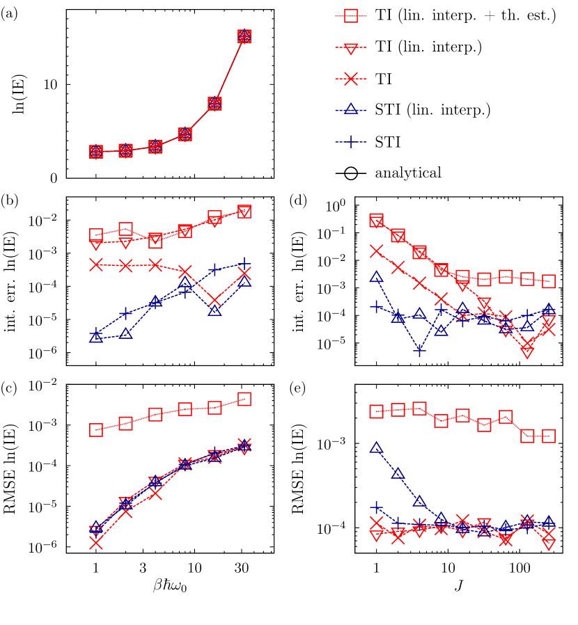
Figure 2: Isotope effect (IE) calculations in an eight-dimensional harmonic model from Subsec. III.2. Unless explicitly stated in the label, all results use the centroid virial estimator (15) and improved mass interpolation (11). Results labeled “lin. interp.” use linear interpolation (10) and those labeled “th. est.” the thermodynamic estimator (14). Several versions of thermodynamic integration (TI) are compared with exact analytical values (for the same finite Trotter number $P$). The proposed method is “stochastic thermodynamics integration” (STI). Panels (a)-(c) show the temperature dependence of (a) the isotope effect, (b) its integration errors, and (c) its statistical root mean square errors (RMSEs). Panels (d)-(e) display the dependence of integration errors and RMSEs on the number $J$ of integration subintervals at a temperature given by $\beta\hbar\omega_{0}=8$.

III.3 Deuteration of methane

III.3.1 Computational details

The methane calculations used the potential energy surface from Ref. Schwenke and Partridge, 2001 and available in the POTLIB library.Duchovic et al. The number of $\lambda$ integration intervals was $J=4$ for TI and $J=4096$ for STI.

TI calculations used a total of $2\times 10^{8}$ Monte Carlo steps which sampled $\mathbf{r}$, for STI the number of $\mathbf{r}$ Monte Carlo steps was $1.8\times 10^{8}$; in both cases $14\%$ were whole-chain moves and $86\%$ were multi-slice moves performed on one sixth of the chain with the staging algorithmSprik, Klein, and Chandler (1985a, b) (this guaranteed that approximately the same computer time was spent on either of the two types of moves). For STI we additionally used $0.2\times 10^{8}$ mass-scaled $\lambda$-moves and $2\times 10^{8}$ simple $\lambda$-moves with $\Delta\lambda_{\mathrm{max}}=0.1$. As the simple $\lambda$-moves are almost free in terms of computational time, the cost of both calculations was still roughly the same. To avoid the unnecessary cost of evaluating correlated samples, all virial estimators were evaluated only after every ten Monte Carlo steps for TI and after every twenty Monte Carlo steps for STI (since STI calculations had twice as many Monte Carlo steps the number of virial estimator samples was still the same), while thermodynamic estimators were evaluated after each step since the CPU time required for their calculation is negligible. The first $20\%$ Monte Carlo steps of each calculation were discarded as “warmup”; as discussed in Subsec. III.1, in the simulations employing the stochastic change of mass, the same warmup period was also used to generate the biasing potential $U_{b}(\lambda)$ needed for the rest of the calculation. The path integral discretization error, estimated by running simulations with a twice larger $P$ at the highest and lowest temperatures ($T=1000\,$K and $T=200\,$K), was below $1\%$; for other temperatures $P$ was obtained by linear interpolation with respect to $1/T$.

Of course, in practice much shorter simulations would be sufficient, but we used overconverged calculations in order to analyze the behavior of different types of errors in detail.

III.3.2 Results and discussion

The results of the calculations of the $\mathrm{CD}_{4}/\mathrm{CH}_{4}$ isotope effect are presented in Fig. 3. Panel (a) shows that the isotope effects calculated with the different methods agree. Yet, a more detailed inspection reveals the improvement provided by the STI compared with the TI. This is done in panel (b), showing the integration errors of the different methods; the STI result with a twice larger value of $J$ (i.e., $J=8192$) is considered as an exact benchmark. In the case of TI the integration error depends strongly on the type of mass interpolation: If the linear interpolation is used, the integration error is even much larger than the statistical error [see panel (c)], while, for this particular system, the improved interpolation (11) of the inverse square root of mass allows to obtain quite accurate results, even though a small integration error remains visible above the statistical noise at higher temperatures. In the case of the STI, on the other hand, no integration error is observed, which was one of the main goals of this work. Finally, panel (c) shows that if the same estimator is used the STI exhibits comparable statistical errors to those of TI, which confirms that employing the STI can easily lower the integration errors without increasing the computational cost.

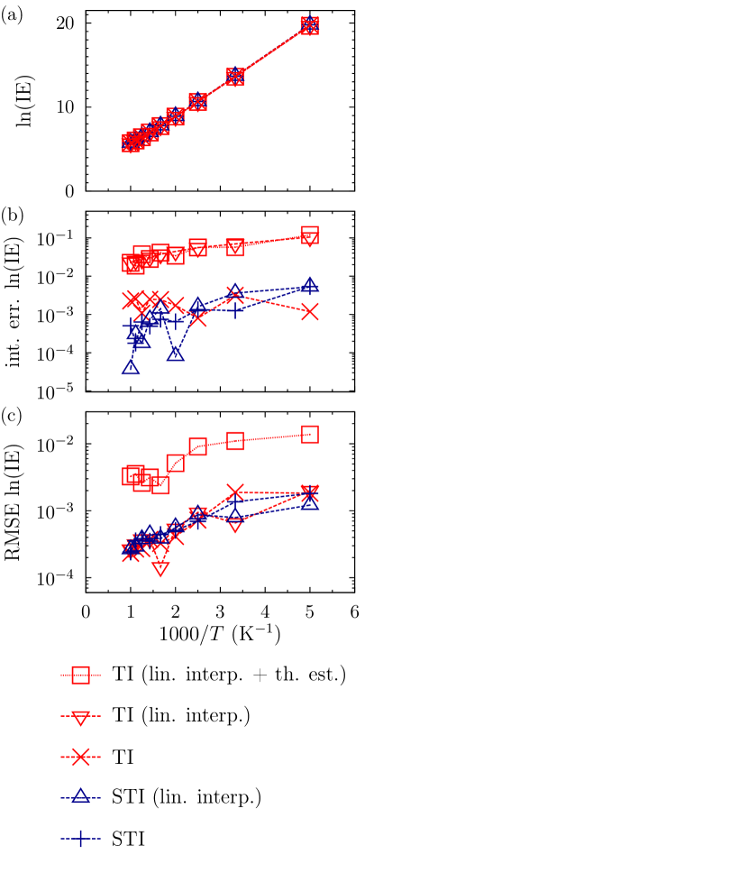
Figure 3: Calculations of the $\mathrm{CD_{4}/CH_{4}}$ isotope effect (IE) from Subsec. III.3. Labels are explained in the caption of Fig. 2. The three panels show the temperature dependence of (a) the isotope effect, (b) its integration errors, and (c) its statistical root mean square errors (RMSEs).

For reference, the plotted values together with their statistical errors are listed in Table 1. From this table it is clear that STI calculations with both types of mass interpolation agree within their statistical errors, while TI, particularly with linear interpolation, retains a significant integration error.

Table 1: Values of the $\mathrm{CD}_{4}/\mathrm{CH}_{4}$ isotope effect (IE) obtained with several versions of thermodynamic integration (TI). Corresponding statistical errors are shown as well. Unless explicitly stated in the label, all results use the centroid virial estimator (15) and improved mass interpolation (11). The proposed methodology is stochastic thermodynamic integration (STI).

$T$	$P$	ln(IE) ($\mathrm{CD_{4}/CH_{4}}$) with statistical error
		TI (lin. interp.	TI (lin. interp.)	TI	STI (lin. interp.)	STI
		+ thermod. est.)
200	360	$19.67\phantom{0}\pm 0.02\phantom{0}$	$19.683\pm 0.002$	$19.785\pm 0.002$	$19.783\pm 0.002$	$19.789\pm 0.002$
300	226	$13.61\phantom{0}\pm 0.01\phantom{0}$	$13.602\pm 0.001$	$13.671\pm 0.002$	$13.676\pm 0.001$	$13.673\pm 0.002$
400	158	$10.61\phantom{0}\pm 0.01\phantom{0}$	$10.612\pm 0.001$	$10.665\pm 0.001$	$10.666\pm 0.001$	$10.667\pm 0.001$
500	118	$\phantom{0}8.876\pm 0.005$	$\phantom{0}8.866\pm 0.001$	$\phantom{0}8.908\pm 0.001$	$\phantom{0}8.910\pm 0.001$	$\phantom{0}8.910\pm 0.001$
600	90	$\phantom{0}7.740\pm 0.003$	$\phantom{0}7.743\pm 0.001$	$\phantom{0}7.778\pm 0.001$	$\phantom{0}7.779\pm 0.001$	$\phantom{0}7.779\pm 0.001$
700	72	$\phantom{0}6.977\pm 0.003$	$\phantom{0}6.974\pm 0.001$	$\phantom{0}7.004\pm 0.001$	$\phantom{0}7.006\pm 0.001$	$\phantom{0}7.006\pm 0.001$
800	58	$\phantom{0}6.413\pm 0.003$	$\phantom{0}6.423\pm 0.001$	$\phantom{0}6.449\pm 0.001$	$\phantom{0}6.451\pm 0.001$	$\phantom{0}6.451\pm 0.001$
900	46	$\phantom{0}6.020\pm 0.003$	$\phantom{0}6.013\pm 0.001$	$\phantom{0}6.037\pm 0.001$	$\phantom{0}6.039\pm 0.001$	$\phantom{0}6.039\pm 0.001$
1000	36	$\phantom{0}5.703\pm 0.003$	$\phantom{0}5.702\pm 0.001$	$\phantom{0}5.723\pm 0.001$	$\phantom{0}5.725\pm 0.001$	$\phantom{0}5.726\pm 0.001$

To better understand the benefit of the STI, recall that stopping a Monte Carlo simulation after obtaining only a finite number of samples introduces two types of errors. The first is the statistical error, which has been analyzed in all calculations so far; the second type is a systematic error, and appears if the sampling procedure yields correlated samples and Monte Carlo trajectories are too short to guarantee ergodicity. This systematic error has not appeared yet since all our calculations were too well converged; however, it becomes important when computational resources are limited, and therefore deserves additional consideration. Indeed, one of the main motivations behind this work was the expectation that equilibrating a single STI simulation should consume fewer computational resources than equilibrating $J$ simulations required in a standard TI calculation. To illustrate this point we ran several much less converged calculations of the $\mathrm{CD}_{4}/\mathrm{CH}_{4}$ isotope effect at $T=200$ K. The number of Monte Carlo steps used during the simulations was doubled from one calculation to the next; for example, for TI there were $1280,2560,...,1310720$ Monte Carlo steps partitioned in the same way as for the more converged calculations. The only difference was that this time no part of the simulation was discarded as warmup. Moreover, to be sure that the error observed for smaller numbers of Monte Carlo steps is the systematic error due to non-ergodicity and not the “true” statistical error, the value obtained with $1280$ Monte Carlo steps was averaged over $4096$ independent calculations, $2560$ - over $2048$ calculations, etc.; this averaging ensured that each result had roughly the same statistical error. The STI calculations were performed with or without the mass-scaled $\lambda$-moves and with or without the simple $\lambda$-moves to compare the efficiency of the resulting methods.

Isotope effects obtained with these much cheaper calculations are compared in Fig. 4, where the converged STI result $\ln\text{IE}=19.789$ from Fig. 3 and Table 1 serves as the exact reference; for a completely fair comparison the results are plotted as a function of the number of potential energy evaluations required to obtain them. As expected, the results of shorter simulations exhibit a significant error due to non-ergodicity of underlying simulations, yet this nonergodicity error is much smaller for the proposed STI than for the TI, making the STI more practical in situations where computational resources are limited. Even though the mass-scaled $\lambda$-moves are quite expensive, their addition accelerates the convergence of the integral. The much cheaper simple $\lambda$-moves appear to also contribute to convergence, as the results obtained without them are not as well converged as results with both types of $\lambda$-moves.

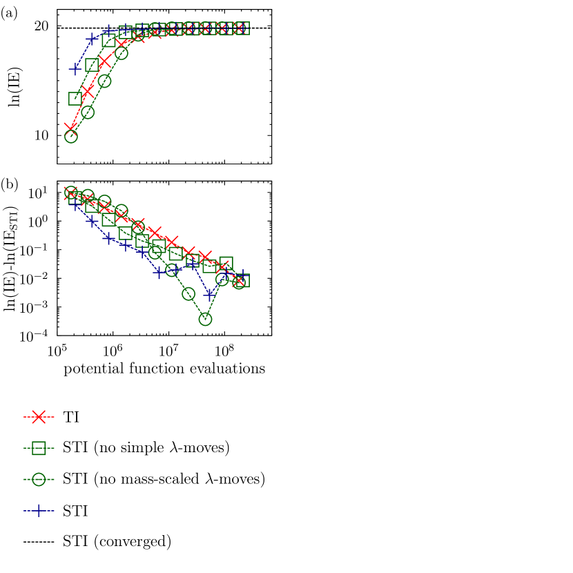
Figure 4: The impact of nonergodicity appearing in shorter calculations of the $\mathrm{CD}_{4}/\mathrm{CH}_{4}$ isotope effect (IE) at $T=200$ K. Panel (a) presents the convergence of the IE as a function of the simulation length, while panel (b) shows the corresponding error of the IE (in logarithmic scale) relative to a converged STI result. Labels TI and STI are as in the caption of Fig. 2; “STI (no simple $\lambda$-moves)” were obtained without the simple $\lambda$-moves defined by Eqs. (19)-(23), while “STI (no mass-scaled $\lambda$-moves)” were obtained without mass-scaled $\lambda$-moves defined by Eqs. (24)-(27). The horizontal line in panel (a) labeled “STI (converged)” is the converged STI result $\ln(\text{IE}_{\mathrm{STI}})=19.789$ from Fig. 3 and Table 1; the same value was used as a reference in panel (b).

IV Conclusion

We have introduced a new Monte Carlo procedure that involves changing atomic masses stochastically during the simulation and allows to eliminate the integration error of thermodynamic integration, thus significantly speeding up isotope effects calculations. The proposed methodology relies on a set of new tools: One of these tools is the introduction of mass-scaled $\lambda$-moves that permit drastic changes of $\lambda$ in a single Monte Carlo step; as shown in Subsec. III.3 their addition can significantly contribute to the convergence of the thermodynamic integral. Another tool is the piecewise linear umbrella biasing potential $U_{b}(\lambda)$ that guarantees a zero integration error of the thermodynamic integral for any number $J$ of integration subintervals; this trick is general and can be used regardless of the type of free energy change one may want to evaluate.

It is possible, as in metadynamics, to facilitate convergence with respect to $\lambda$ by additionally biasing the simulation with a history-dependent potential that pushes the system into less explored regions of configuration space; this addition can become important if the change of isotope masses $m_{i}(\lambda)$ is so drastic that one has to impose an upper bound $\Delta\lambda_{\mathrm{max}}$ for the change of $\lambda$ in a single step even for the mass-scaled $\lambda$-moves. However, this did not occur in systems considered in this work, where mass-scaled $\lambda$-moves yielded acceptance probabilities above $70\%$ in all calculations. As a result, the mass-scaled $\lambda$-moves allowed large changes of $\lambda$ in a single step, leading to a fast convergence over the $\lambda$ dimension without additional modifications of the Monte Carlo procedure.

In this work we relied heavily on the fact that $\lambda$ values can be sampled without repercussions even if they are placed far away from the endpoints $\lambda=0$ and $\lambda=1$ that correspond to physically meaningful systems. This is true for IEs, as also found in Ref. Pérez and von Lilienfeld, 2011, but may not be so for other calculations of free energy differences. As a result, several variants of $\lambda$-dynamics bias the sampling of $\lambda$ towards the endpoints, and then calculate the free energy difference from the ratio of probability densities at $\lambda=0$ and $\lambda=1$.Abrams, Rosso, and Tuckerman (2006); Wu, Hu, and Yang (2011) Indeed, our STI approach would also allow obtaining a well converged result by sampling mainly in the regions of $\lambda$ close to the endpoints $\lambda=0$ and $\lambda=1$ if one used a modified partition function

$$\tilde{Q}(\lambda)=Q(\lambda)e^{-\beta V_{\mathrm{barr}}(\lambda)},$$ (34)

where $V_{\mathrm{barr}}(\lambda)$ is a potential that biases the Monte Carlo chain towards the end points. Running an STI calculation with $J=1$ will lead to an exact partition function ratio and at the same time use mainly samples from values of $\lambda$ close to the endpoints. Although such an approach would avoid the problem of choosing an optimal bin width for the weighted histogram analysis method (WHAM), an issue discussed in Ref. Kästner and Thiel, 2005, it would, just as WHAM, require equilibration over the entire $\lambda$ interval $[0,1]$ instead of only over each subinterval $I_{j}$, which would make it less convenient than the simple STI presented.

We would also like to mention an alternative approach allowing to remove the integration error of the isotope effect entirely, which was proposed recently by Cheng and CeriottiCheng and Ceriotti (2015) and is a variant of the free energy perturbation method.Ceriotti and Markland (2013) Cheng and Ceriotti’s approach employs so-called “direct estimators” and is particularly suitable for isotope effects close to unity, which occur frequently, e.g., in the condensed phase, where only a small fraction of molecules is isotopically substituted. However, for large isotope effects, such as those discussed here, the direct estimators tend to have large statistical errors. In the future,Karandashev and Vaníček we therefore plan to combine the trick of a stochastic mass change with the direct estimators, in order to make the latter method practical for large isotope effects as well.

Let us conclude by noting that the stochastic thermodynamic integration can be combined with Takahashi-Imada or Suzuki fourth-order factorizationsTakahashi and Imada (1984); Suzuki (1995); Chin (1997); Jang, Jang, and Voth (2001) of the Boltzmann operator, which would allow lowering the path integral discretization error of the computed isotope effect for a given Trotter number $P$, and hence a faster convergence to the quantum limit. The combination of higher-order path integral splittings with standard thermodynamic integration has been discussed elsewhere;Pérez and Tuckerman (2011); Buchowiecki and Vaníček (2013); Maršálek et al. (2014); Karandashev and Vaníček (2015) as for the extension to stochastic thermodynamic integration, the main additional change consists in replacing the potential $V$ in the acceptance probability in Eq. (27) with an effective potential depending on mass and, in the case of the fourth-order Suzuki splitting, in an additional factor depending on the imaginary time-slice index $s$.

Appendix A Mass-scaled normal modes of the ring polymer and the derivation of the virial estimator and mass-scaled $\lambda$-move

In this appendix we outline how transforming from Cartesian coordinates to mass-scaled normal modes of the ring polymerCoalson, Freeman, and Doll (1986); Cao and Berne (1993) leads to simple derivations of the centroid virial estimator $\left[dF(\lambda)/d\lambda\right]_{\text{cv}}$ [Eq. (15) from Subsec. II.2] and the mass-scaled trial move with respect to the mass parameter $\lambda$ [Eqs. (24)-(27) from Subsec. II.3].

The mass-scaled normal mode coordinates $\mathbf{a}=\{\mathbf{a}^{(1)},\ldots,\mathbf{a}^{(P/2)}\}$ and $\mathbf{b}=\{\mathbf{b}^{(1)},\ldots,\mathbf{b}^{(P/2-1)}\}$ can be obtained as

$$\mathrm{a}_{i}^{(k)} =\frac{\sqrt{m_{i}}}{P}\sum_{s=1}^{P}\mathrm{r}_{i}^{(s)}\cos\left(\frac{2\pi sk}{P}\right),\,k\in\{1,2,\ldots,P/2\}$$ (35)

$$\mathrm{b}_{i}^{(l)} =\frac{\sqrt{m_{i}}}{P}\sum_{s=1}^{P}\mathrm{r}_{i}^{(s)}\sin\left(\frac{2\pi sl}{P}\right),\,l\in\{1,2,\ldots,P/2-1\},$$ (36)

where $\mathrm{a}_{i}^{(k)}$ and $\mathrm{b}_{i}^{(l)}$ are components of $\mathbf{a}^{(k)}$ and $\mathbf{b}^{(l)}$ corresponding to particle $i$. This set of coordinates becomes complete after adding the centroid $\mathbf{r}^{(C)}=P^{-1}\sum_{s=1}^{P}\mathbf{r}^{(s)}$, which can also be thought of as the zero-frequency normal mode, and we will refer to the triple $(\mathbf{a},\mathbf{b},\mathbf{r}^{(C)})$ simply as $\mathbf{u}$. Note that, for convenience, we have not mass-scaled $\mathbf{r}^{(C)}$. For simplicity, we only consider even values of the Trotter number $P$ since the case of odd $P$ differs in minor details but is otherwise completely analogous.

The original coordinates $\mathbf{r}$ are recovered from the normal mode coordinates $\mathbf{u}$ via the inverse transformation

$$\mathrm{r}_{i}^{(s)}=\mathrm{r}_{i}^{(C)}+\frac{1}{\sqrt{m_{i}}}\left\{(-1)^{s}\mathrm{a}_{i}^{(P/2)}+2\sum_{k=1}^{P/2-1}\left[\mathrm{a}_{i}^{(k)}\cos\left(\frac{2\pi sk}{P}\right)+\mathrm{b}_{i}^{(k)}\sin\left(\frac{2\pi sk}{P}\right)\right]\right\}$$ (37)

with the Jacobian

$$J=\frac{P^{NDP/2}\cdot 2^{ND(P/2-1)}}{\left(\prod_{i=1}^{N}m_{i}\right)^{D(P-1)/2}}.$$ (38)

These two expressions can be obtained easily starting from properties of the real version of the Discrete Fourier Transform.Ersoy (1985)

Rewriting the path integral representation of the partition function in terms of the normal-mode coordinates leads to

$$Q_{P} =\int d\mathbf{u}\tilde{\rho}(\mathbf{u})\text{,}$$ (39)

$$\tilde{\rho} =\tilde{C}\exp\left[-\beta\tilde{\Phi}(\mathbf{u})\right],$$ (40)

where the new effective potential $\tilde{\Phi}(\mathbf{u})$ and normalization constant $\tilde{C}$ are given by

$$\tilde{\Phi}:= \frac{2P^{2}}{\beta^{2}\hbar^{2}}\left\{|\mathbf{a}^{(P/2)}|^{2}+\sum_{k=1}^{P/2-1}(|\mathbf{a}^{(k)}|^{2}+|\mathbf{b}^{(k)}|^{2})\left[1-\cos\left(\frac{2\pi k}{P}\right)\right]\right\}$$

$$+\frac{1}{P}\sum_{s=1}^{P}V\left[\mathbf{r}^{(s)}(\mathbf{u},\{m_{i}\})\right],$$ (41)

$$\tilde{C}:= \left(\frac{P^{2}}{\beta\hbar^{2}\pi}\right)^{NDP/2}\frac{\left(\prod_{i=1}^{N}m_{i}\right)^{D/2}}{2^{ND}}.$$ (42)

Note that the only term of $\tilde{\Phi}(\mathbf{u})$ depending on mass is the average of $V(\mathbf{r}^{(s)})$ over the $P$ beads.

With this setup, the centroid virial estimator (15) can be obtained immediately by differentiating the right-hand side of Eq. (40) with respect to $\lambda$. To derive the mass-scaled $\lambda$-move described by Eqs. (24)-(27), we consider making a trial move with respect to $\lambda$ with $\tilde{\rho}^{(\lambda)}(\mathbf{u})$ as the probability density while keeping $\mathbf{u}$ constant. Transforming the corresponding ratio of probability densities

$$\begin{split}\frac{\tilde{\rho}^{(\lambda^{\prime\prime})}(\mathbf{u})}{\tilde{\rho}^{(\lambda^{\prime})}(\mathbf{u})}=&\left[\prod_{i=1}^{N}\frac{m_{i}(\lambda^{\prime\prime})}{m_{i}(\lambda^{\prime})}\right]^{D/2}\\ &\times\exp\left(\frac{\beta}{P}\sum_{s=1}^{P}\{V[\mathbf{r}^{(s)}(\mathbf{u},\{m_{i}(\lambda^{\prime})\})]-V[\mathbf{r}^{(s)}(\mathbf{u},\{m_{i}(\lambda^{\prime\prime})\})]\}\right)\end{split}$$ (43)

back to Cartesian coordinates $\mathbf{r}$ will immediately yield Eq. (27).

Finally, let us remark that the algorithm used in Subsec. III.2 for sampling the harmonic system also uses normal modes of the ring polymer, albeit not scaled by mass.

Appendix B Dependence of the error of stochastic thermodynamic integration on the choice of umbrella biasing potential

In this appendix we discuss how one may minimize the numerical errors appearing if the IE is evaluated with STI [via Eq. (30)] by an appropriate choice of the umbrella potential. The two errors introduced by the procedure are the statistical error and integration error due to a finite value of $J$. To estimate the integration error, we note that $U_{b}(\lambda)$ is independent of $\mathbf{r}$ and rewrite $\langle[dF(\lambda)/d\lambda]_{\mathrm{cv}}\rangle^{I_{j}}$ as

$$\begin{split}\left\langle[dF(\lambda)/d\lambda]_{\mathrm{cv}}\right\rangle^{I_{j}}=&\frac{\int_{\lambda_{j-1}}^{\lambda_{j}}d\lambda\int d\mathbf{r}\rho^{(\lambda)}(\mathbf{r})[dF(\lambda)/d\lambda]_{\mathrm{cv}}\exp[-\beta U_{b}(\lambda)]}{\int_{\lambda_{j-1}}^{\lambda_{j}}d\lambda\int d\mathbf{r}\rho^{(\lambda)}(\mathbf{r})\exp[-\beta U_{b}(\lambda)]}\\ =&\frac{\int_{\lambda_{j-1}}^{\lambda_{j}}d\lambda\exp[-\beta U_{b}(\lambda)]\int d\mathbf{r}\rho^{(\lambda)}(\mathbf{r})[dF(\lambda)/d\lambda]_{\mathrm{cv}}}{\int_{\lambda_{j-1}}^{\lambda_{j}}d\lambda\exp[-\beta U_{b}(\lambda)]\int d\mathbf{r}\rho^{(\lambda)}(\mathbf{r})}\\ =&-\frac{\int_{\lambda_{j-1}}^{\lambda_{j}}d\lambda\exp[-\beta U_{b}(\lambda)+\ln Q(\lambda)]d\ln Q(\lambda)/d\lambda}{\beta\int_{\lambda_{j-1}}^{\lambda_{j}}d\lambda\exp[-\beta U_{b}(\lambda)+\ln Q(\lambda)]}.\end{split}$$ (44)

Now let us consider several possible choices for the umbrella potential; an impatient reader should skip the subsection on a piecewise constant umbrella potential since we show that the most useful in practice is the piecewise linear umbrella potential.

B.1 Exact umbrella potential

Suppose that one can find the ideal, “exact” umbrella potential

$$U_{b,\mathrm{exact}}(\lambda):=\beta^{-1}\ln Q(\lambda).$$ (45)

Using this exact umbrella potential amounts to the substitution $U_{b}(\lambda)=U_{b,\mathrm{exact}}(\lambda)$ in Eq. (44) and gives

$$\left\langle[dF(\lambda)/d\lambda]_{\mathrm{cv}}\right\rangle^{I_{j}}=-\frac{\ln Q(\lambda_{j})-\ln Q(\lambda_{j-1})}{\beta(\lambda_{j}-\lambda_{j-1})}.$$ (46)

Since $\lambda_{j}-\lambda_{j-1}=J^{-1}$, in this ideal situation Eq. (30) will yield the exact partition function ratio at any value of $J$.

B.2 Piecewise constant umbrella potential

Unfortunately, in a realistic calculation this ideal potential $U_{b,\text{exact}}(\lambda)$ is not available and one must make do with an approximation. The simplest choice is a piecewise constant potential

$$U_{b,\mathrm{p.const.}}(\lambda):=U_{b,j}\text{ for }\lambda\in(\lambda_{j},\lambda_{j-1}).$$ (47)

To simplify the following algebra we introduce a symbol

$$\Delta(\lambda):=\ln Q(\lambda)-\ln Q(\overline{\lambda}_{j})$$ (48)

and note that after the substitution $U_{b}(\lambda)=U_{b,\mathrm{p.const.}}(\lambda)$ the constant factor $\exp[-\beta U_{b,j}+\ln Q(\overline{\lambda}_{j})]$ will cancel out between the numerator and denominator of Eq. (44), leading to a simplified expression

$$\left\langle[dF(\lambda)/d\lambda]_{\mathrm{cv}}\right\rangle^{I_{j}}=-\frac{\int_{\lambda_{j-1}}^{\lambda_{j}}d\lambda\exp[\Delta(\lambda)]d\ln Q(\lambda)/d\lambda}{\beta\int_{\lambda_{j-1}}^{\lambda_{j}}d\lambda\exp[\Delta(\lambda)]}.$$ (49)

Although it was not important for the derivation of the last equation, it is worthwhile to mention that the constants $U_{b,j}$ are determined in the simulation from the equation

$$U_{b,j+1}=U_{b,j}+\frac{\left\langle[dF(\lambda)/d\lambda]_{\mathrm{cv}}\right\rangle^{I_{j}}+\left\langle[dF(\lambda)/d\lambda]_{\mathrm{cv}}\right\rangle^{I_{j+1}}}{2J}.$$ (50)

Upon changing variables from $\lambda$ to $\Delta(\lambda)$, the numerator of Eq. (49) becomes

$$\int_{\Delta(\lambda_{j-1})}^{\Delta(\lambda_{j})}e^{\Delta(\lambda)}d\Delta(\lambda)=e^{\Delta(\lambda_{j})}-e^{\Delta(\lambda_{j-1})},$$ (51)

hence

$$\left\langle[dF(\lambda)/d\lambda]_{\mathrm{cv}}\right\rangle^{I_{j}}=-\frac{f(\lambda_{j})-f(\lambda_{j-1})}{\beta\int_{\lambda_{j-1}}^{\lambda_{j}}[1+f(\lambda)]d\lambda},$$ (52)

where we defined a function

$$f(\lambda):=e^{\Delta(\lambda)}-1,$$ (53)

whose Taylor series expansion about $\overline{\lambda}_{j}$,

$$f(\lambda)=f^{\prime}(\overline{\lambda}_{j})(\lambda-\overline{\lambda}_{j})+\frac{f^{\prime\prime}(\overline{\lambda}_{j})}{2}(\lambda-\overline{\lambda}_{j})^{2}+\frac{f^{\prime\prime\prime}(\overline{\lambda}_{j})}{6}(\lambda-\overline{\lambda}_{j})^{3}+\mathcal{O}[(\lambda-\overline{\lambda}_{j})^{4}],$$ (54)

will be used in the following. To see how good an approximation the piecewise constant potential gives, let us compare the numerators and denominators of Eqs. (46) and (52). The difference of the denominators is

$$\beta\int_{\lambda_{j-1}}^{\lambda_{j}}[1+f(\lambda)]d\lambda-\beta(\lambda_{j}-\lambda_{j-1})=\frac{\beta f^{\prime\prime}(\overline{\lambda}_{j})}{24J^{3}}+\mathcal{O}(J^{-4}).$$ (55)

Noting that $f(\lambda)=\mathcal{O}(\lambda-\overline{\lambda}_{j})$ and Taylor expanding the logarithm, we find the difference of the numerators to be

$$\begin{split}&f(\lambda_{j})-f(\lambda_{j-1})-\ln[1+f(\lambda_{j})]+\ln[1+f(\lambda_{j-1})]\\ =&\frac{f(\lambda_{j})^{2}-f(\lambda_{j-1})^{2}}{2}-\frac{f(\lambda_{j})^{3}-f(\lambda_{j-1})^{3}}{3}+\mathcal{O}(J^{-4})\\ =&\frac{[f(\lambda_{j})-f(\lambda_{j-1})][f(\lambda_{j})+f(\lambda_{j-1})]}{2}\\ &-\frac{f^{\prime}(\overline{\lambda}_{j})^{3}(\lambda_{j}-\lambda_{j-1})^{3}}{12}+\mathcal{O}(J^{-4})\\ =&\frac{f^{\prime}(\overline{\lambda}_{j})f^{\prime\prime}(\overline{\lambda}_{j})}{8J^{3}}-\frac{f^{\prime}(\overline{\lambda}_{j})^{3}}{12J^{3}}+\mathcal{O}(J^{-4}).\end{split}$$ (56)

Since both the numerator and denominator of Eq. (46) are $\mathcal{O}(J^{-1})$, and since the errors in Eq. (52) of both the denominator [Eq. (55)] and numerator [Eq. (56)] are $\mathcal{O}(J^{-3})$, the overall error is $\mathcal{O}(J^{-2})$, that is, for an umbrella potential constant over each $I_{j}$

$$\langle[dF(\lambda)/d\lambda]_{\mathrm{cv}}\rangle^{I_{j}}=-\frac{\ln Q(\lambda_{j})-\ln Q(\lambda_{j-1})}{\beta(\lambda_{j}-\lambda_{j-1})}+\mathcal{O}(J^{-2}).$$ (57)

In conclusion, for the piecewise constant biasing potential Eq. (30) will have an error $\mathcal{O}(J^{-2})$:

$$\exp\left\{-\frac{\beta}{J}\sum_{j=1}^{J}\left\langle\left[dF(\lambda)/d\lambda\right]_{\text{cv}}\right\rangle^{I_{j}}\right\}=\frac{Q_{P}^{(B)}}{Q_{P}^{(A)}}+\mathcal{O}(J^{-2}).$$ (58)

As discussed in Subsec. (II.3), it is easy to use really large values of $J$ during the calculation, therefore an $\mathcal{O}(J^{-2})$ error is not an issue. Yet, it is still worthwhile to try to optimize the procedure in order to go beyond an $\mathcal{O}(J^{-2})$ error.

B.3 Piecewise linear umbrella potential

The obvious “first” improvement is introducing a piecewise linear potential. A remarkable fact about the resulting procedure is that it yields an exactly zero integration error, and this is true to all orders in $J$. Indeed, if we introduce a $U_{b}(\lambda)=U_{b,\mathrm{p.lin.}}(\lambda)$, where

$$U_{b,\mathrm{p.lin.}}(\lambda):=U_{b,j}-\langle[dF(\lambda)/d\lambda]_{\mathrm{cv}}\rangle^{I_{j}}(\lambda-\overline{\lambda}_{j}),$$ (59)

then the constant factor $\exp(-\beta\{U_{b,j}-\langle[dF(\lambda)/d\lambda]_{\mathrm{cv}}\rangle^{I_{j}}\overline{\lambda}_{j}\})$ will cancel between the numerator and denominator of Eq. (44), giving

$$\left\langle[dF(\lambda)/d\lambda]_{\mathrm{cv}}\right\rangle^{I_{j}}=-\frac{\int_{\lambda_{j-1}}^{\lambda_{j}}d\lambda\exp\{\beta\langle[dF(\lambda)/d\lambda]_{\mathrm{cv}}\rangle^{I_{j}}\lambda+\ln Q(\lambda)\}d\ln Q(\lambda)/d\lambda}{\beta\int_{\lambda_{j-1}}^{\lambda_{j}}d\lambda\exp\{\beta\langle[dF(\lambda)/d\lambda]_{\mathrm{cv}}\rangle^{I_{j}}\lambda+\ln Q(\lambda)\}}.$$ (60)

Multiplying both sides of the equation by the denominator and rearranging yields an identity

$$0 =\int_{\lambda_{j-1}}^{\lambda_{j}}\exp\{\beta\langle[dF(\lambda)/d\lambda]_{\mathrm{cv}}\rangle^{I_{j}}\lambda+\ln Q(\lambda)\}\{\beta\left\langle[dF(\lambda)/d\lambda]_{\mathrm{cv}}\right\rangle^{I_{j}}d\lambda+d\ln Q(\lambda)\}$$ (61)

$$=\int_{g(\lambda_{j-1})}^{g(\lambda_{j})}dg(\lambda)e^{g(\lambda)}=e^{g(\lambda_{j})}-e^{g(\lambda_{j-1})},$$ (62)

where we have introduced a function $g(\lambda):=\beta\langle[dF(\lambda)/d\lambda]_{\mathrm{cv}}\rangle^{I_{j}}\lambda+\ln Q(\lambda)$. The last equality means $g(\lambda_{j})=g(\lambda_{j-1})$, leading to

$$\langle[dF(\lambda)/d\lambda]_{\mathrm{cv}}\rangle^{I_{j}}=-\frac{\ln Q(\lambda_{j})-\ln Q(\lambda_{j-1})}{\beta(\lambda_{j}-\lambda_{j-1})},$$ (63)

which is, remarkably, the same as Eq. (46) for the exact umbrella potential.

Of course, the definition of the piecewise linear umbrella potential in Eq. (59) is recursive, and therefore can only be evaluated by an iterative algorithm, but this should not cause a great concern since any biasing potential $U_{b}(\lambda)$, regardless of its type, cannot be known a priori (in particular, even the piecewise constant umbrella potential must be constructed iteratively).

As already mentioned in Subsec. (II.3), making $U_{b}(\lambda)$ not only piecewise linear [by satisfying Eq. (59)] but also continuous [by choosing the constants $U_{b,j}$ from Eq. (50)] allows to approach an optimal statistical error. An analytical analysis of the statistical error is more involved; instead, in the following subsection we show numerically that the statistical error is approximately independent of the choice of the umbrella potential and converges to a limit as $J$ is increased—in particular, the piecewise linear umbrella potential permits reducing the integration to zero without increasing the statistical error.

B.4 Numerical tests

As the piecewise linear umbrella potential $U_{b,\mathrm{p.lin.}}(\lambda)$ defined by Eq. (31) yields a zero integration error and can be obtained iteratively in any system, it was this potential that was used in the production runs in the rest of the paper. To clearly demonstrate the advantages of $U_{b,\mathrm{p.lin.}}(\lambda)$, in this subsection we compare the different choices of the umbrella potential on the harmonic system from Subsec. III.2, for which which even the exact umbrella potential (45) is available since $Q(\lambda)$ is known analytically.

The results are presented in Fig. 5, which shows the dependence of integration and statistical errors on $J$. [Note that all methods employed the linear interpolation of mass given by Eq. (10) and that the values obtained with TI and with STI with a piecewise linear potential are the same as those already presented in Subsec. III.2.]

As predicted above, the integration error of STI appears to be zero for both the ideal, exact umbrella potential (45) and for the piecewise linear umbrella potential (59) [panels (a) and (b)], whereas both TI with the midpoint rule and STI with the piecewise constant umbrella potential (47) exhibit an $\mathcal{O}(J^{-2})$ integration error [panel (b)]. Note that for a given $J$ the integration error of STI with the piecewise constant potential is even larger than the error of TI using the midpoint rule; however, this does not imply that STI is less efficient than TI since in realistic calculations STI can be used with much larger values of $J$ than TI, without increasing the statistical error or the computational cost. Finally, note that the different choices of the umbrella potential do not significantly affect the statistical error [see panel (c)].

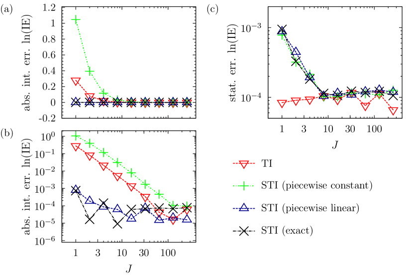
Figure 5: Impact of the umbrella biasing potential on the numerical errors of a simulation. The figure shows the dependence of integration errors [(a) with linear, (b) with logarithmic scale] and statistical errors [panel (c)] on the number $J$ of $\lambda$ intervals used in the standard thermodynamic integration (TI) and stochastic thermodynamic integration (STI) employing various types of umbrella potentials mentioned in parentheses: “piecewise constant” uses an umbrella potential (47) constant over each of the $J$ intervals, “piecewise linear” potential is given by Eqs. (31) or (59), and “exact” corresponds to the unrealistic situation when one knows the exact, ideal umbrella potential (45).

References

- Wolfsberg et al. (2010) M. Wolfsberg, W. A. V. Hook, P. Paneth, and L. P. N. Rebelo, Isotope Effects in the Chemical, Geological and Bio Sciences (McGraw-Hill, 2010).
- Urey (1947) H. C. Urey, J. Chem. Soc. 1947, 562 (1947).
- McKenzie, Athokpam, and Ramesh (2015) R. M. McKenzie, B. Athokpam, and S. G. Ramesh, J. Chem. Phys. 143, 044309 (2015).
- Janak and Parkin (2003) K. E. Janak and G. Parkin, J. Am. Chem. Soc. 125, 13219 (2003).
- Webb and Miller III (2014) M. A. Webb and T. F. Miller III, J. Phys. Chem. A 118, 467 (2014).
- Richet, Bottinga, and Javoy (1977) P. Richet, Y. Bottinga, and M. Javoy, Ann. Rev. Earth Planet. Sci. 5, 65 (1977).
- Barone (2004) V. Barone, J. Chem. Phys. 120, 3059 (2004).
- Liu, Tossell, and Liu (2010) Q. Liu, J. A. Tossell, and Y. Liu, Geochim. Cosmochim. Acta 74, 6965 (2010).
- Feynman and Hibbs (1965) R. P. Feynman and A. R. Hibbs, Quantum mechanics and path integrals (McGraw-Hill, 1965).
- Chandler and Wolynes (1981) D. Chandler and P. G. Wolynes, J. Chem. Phys. 74, 4078 (1981).
- Ceperley (1995) D. M. Ceperley, Rev. Mod. Phys. 67, 279 (1995).
- Kirkwood (1935) J. G. Kirkwood, J. Chem. Phys. 3, 300 (1935).
- Frenkel and Smit (2002) D. Frenkel and B. Smit, Understanding Molecular Simulation (Academic Press, 2002).
- Tuckerman (2010) M. E. Tuckerman, Statistical Mechanics: Theory and Molecular Simulation (Oxford University Press, 2010).
- Vaníček et al. (2005) J. Vaníček, W. H. Miller, J. F. Castillo, and F. J. Aoiz, J. Chem. Phys. 123, 054108 (2005).
- Vaníček and Miller (2007) J. Vaníček and W. H. Miller, J. Chem. Phys. 127, 114309 (2007).
- Zimmermann and Vaníček (2009) T. Zimmermann and J. Vaníček, J. Chem. Phys. 131, 024111 (2009).
- Zimmermann and Vaníček (2010) T. Zimmermann and J. Vaníček, J. Mol. Model. 16, 1779 (2010).
- Pérez and von Lilienfeld (2011) A. Pérez and O. A. von Lilienfeld, J. Chem. Theory Comput. 7, 2358 (2011).
- Ceriotti and Markland (2013) M. Ceriotti and T. E. Markland, J. Chem. Phys. 138, 014112 (2013).
- Maršálek et al. (2014) O. Maršálek, P.-Y. Chen, R. Dupuis, M. Benoit, M. Méheut, Z. Bačić, and M. E. Tuckerman, J. Chem. Theory Comput. 10, 1440 (2014).
- Liu and Berne (1993) Z. Liu and B. J. Berne, J. Chem. Phys. 99, 6071 (1993).
- Kong and Brooks III (1996) X. Kong and C. L. Brooks III, J. Chem. Phys. 105, 2414 (1996).
- Guo, Brooks III, and Kong (1998) Z. Guo, C. L. Brooks III, and X. Kong, J. Phys. Chem. B 102, 2032 (1998).
- Bitetti-Putzer, Yang, and Karplus (2003) R. Bitetti-Putzer, W. Yang, and M. Karplus, Chem. Phys. Lett. 377, 633 (2003).
- Osawa et al. (2010) T. Osawa, T. Futakuchi, T. Imahori, and I.-Y. S. Lee, J. Mol. Catal. A 320, 68 (2010).
- Hargreaves et al. (2002) J. S. J. Hargreaves, G. J. Hutchings, R. W. Joyner, and S. H. Taylor, Appl. Catal. A 227, 191 (2002).
- Lynch, Mielke, and Truhlar (2005) V. A. Lynch, S. L. Mielke, and D. G. Truhlar, J. Phys. Chem 109, 10092 (2005).
- Predescu and Doll (2002) C. Predescu and J. D. Doll, J. Chem. Phys. 117, 7448 (2002).
- Yamamoto (2005) T. Yamamoto, J. Chem. Phys. 123, 104101 (2005).
- Kästner and Thiel (2005) J. Kästner and W. Thiel, J. Chem. Phys. 123, 144104 (2005).
- Kästner (2009) J. Kästner, J. Chem. Phys. 131, 034109 (2009).
- Kästner (2012) J. Kästner, J. Chem. Phys. 136, 234102 (2012).
- Darve and Pohorille (2001) E. Darve and A. Pohorille, J. Chem. Phys. 115, 9169 (2001).
- Darve, Rodrígues-Gómez, and Pohorille (2008) E. Darve, D. Rodrígues-Gómez, and A. Pohorille, J. Chem. Phys. 128, 144120 (2008).
- Comer et al. (2015) J. Comer, J. C. Gumbart, J. Hénin, T. Lelièvre, A. Pohorille, and C. Chipot, J. Phys. Chem. B 119, 1129 (2015).
- Mezei (1987) M. Mezei, J. Comput. Phys. 68, 237 (1987).
- Hooft, van Eijck, and Kroon (1992) R. W. W. Hooft, B. P. van Eijck, and J. Kroon, J. Chem. Phys. 97, 6690 (1992).
- Bartels and Karplus (1997) C. Bartels and M. Karplus, J. Comput. Chem. 18, 1450 (1997).
- Micheletti, Laio, and Parrinello (2004) C. Micheletti, A. Laio, and M. Parrinello, Phys. Rev. Lett. 92, 170601 (2004).
- Laio et al. (2005) A. Laio, A. Rodriguez-Fortea, F. L. Gervasio, M. Ceccarelli, and M. Parrinello, J. Phys. Chem. B 109, 6714 (2005).
- Schweizer et al. (1981) K. S. Schweizer, R. M. Stratt, D. Chandler, and P. G. Wolynes, J. Chem. Phys. 75, 1347 (1981).
- Flyvbjerg and Petersen (1989) H. Flyvbjerg and H. G. Petersen, J. Chem. Phys. 91, 461 (1989).
- Herman, Bruskin, and Berne (1982) M. F. Herman, E. J. Bruskin, and B. J. Berne, J. Chem. Phys. 76, 5150 (1982).
- Cao and Berne (1993) J. Cao and B. J. Berne, J. Chem. Phys. 99, 2902 (1993).
- Schwenke and Partridge (2001) D. W. Schwenke and H. Partridge, Spectrochim. Acta A 57, 887 (2001).
- (47) R. J. Duchovic, Y. L. Volobuev, G. C. Lynch, A. W. Jasper, D. G. Truhlar, T. C. Allison, A. F. Wagner, B. C. Garrett, J. Espinosa-García, and J. C. Corchado, POTLIB, http://comp.chem.umn.edu/potlib.
- Sprik, Klein, and Chandler (1985a) M. Sprik, M. L. Klein, and D. Chandler, Phys. Rev. B 31, 4234 (1985a).
- Sprik, Klein, and Chandler (1985b) M. Sprik, M. L. Klein, and D. Chandler, Phys. Rev. B 32, 545 (1985b).
- Abrams, Rosso, and Tuckerman (2006) J. B. Abrams, L. Rosso, and M. E. Tuckerman, J. Chem. Phys. 125, 074115 (2006).
- Wu, Hu, and Yang (2011) P. Wu, X. Hu, and W. Yang, J. Phys. Chem. Lett. 2, 2099 (2011).
- Cheng and Ceriotti (2015) B. Cheng and M. Ceriotti, J. Chem. Phys. 141, 244112 (2015).
- (53) K. Karandashev and J. Vaníček, “Accelerating equilibrium isotope effect calculations: II. stochastic implementation of direct estimators,” J. Chem. Phys., in preparation.
- Takahashi and Imada (1984) M. Takahashi and M. Imada, J. Phys. Soc. Jpn. 53, 963 (1984).
- Suzuki (1995) M. Suzuki, Physics Letters A 201, 425 (1995).
- Chin (1997) S. A. Chin, Phys. Lett. A 226, 344 (1997).
- Jang, Jang, and Voth (2001) S. Jang, S. Jang, and G. A. Voth, J. Chem. Phys. 115, 7832 (2001).
- Pérez and Tuckerman (2011) A. Pérez and M. E. Tuckerman, J. Chem. Phys. 135, 064104 (2011).
- Buchowiecki and Vaníček (2013) M. Buchowiecki and J. Vaníček, Chem. Phys. Lett. 588, 11 (2013).
- Karandashev and Vaníček (2015) K. Karandashev and J. Vaníček, J. Chem. Phys. 143, 194104 (2015).
- Coalson, Freeman, and Doll (1986) R. D. Coalson, D. L. Freeman, and J. D. Doll, J. Chem. Phys. 85, 4567 (1986).
- Ersoy (1985) O. Ersoy, IEEE Trans. Acoust., Speech, Signal Process. 33, 880 (1985).