Accelerating quantum instanton calculations of the kinetic isotope effects

Abstract

Path integral implementation of the quantum instanton approximation currently belongs among the most accurate methods for computing quantum rate constants and kinetic isotope effects, but its use has been limited due to the rather high computational cost. Here we demonstrate that the efficiency of quantum instanton calculations of the kinetic isotope effects can be increased by orders of magnitude by combining two approaches: The convergence to the quantum limit is accelerated by employing high-order path integral factorizations of the Boltzmann operator, while the statistical convergence is improved by implementing virial estimators for relevant quantities. After deriving several new virial estimators for the high-order factorization and evaluating the resulting increase in efficiency, using $\mathrm{\cdot H_{\alpha}+H_{\beta}H_{\gamma}\rightarrow H_{\alpha}H_{\beta}+\cdot H_{\gamma}}$ reaction as an example, we apply the proposed method to obtain several kinetic isotope effects on $\mathrm{CH_{4}+\cdot H\rightleftharpoons\cdot CH_{3}+H_{2}}$ forward and backward reactions.

I Introduction

Accurate evaluation of the rate constant, i.e., the prefactor of the rate law of elementary chemical reactions, remains one of the central goals of chemical kinetics because this constant reflects the mechanism of the reaction as well as other properties of the potential energy surface on which the reaction occurs. Another quantity that is frequently used for studying reaction mechanisms, and, in particular, detecting nuclear quantum effects on reaction rates, is the kinetic isotope effect (KIE). The KIE is defined as the ratio of rate constants for two isotopologs, i.e., molecules that only differ in isotope composition. These effects, which include, e.g., tunneling, corner-cutting, and zero-point energy effect, tend to play an important role in hydrogen transfer reactions with a high activation barrier. Although they are most important at low temperatures, nuclear quantum effects sometimes manifest themselves even at physiological temperatures, a fact uncovered by studying KIE’s on some enzymatic reactions.Sen and Kohen (2010)

Several approaches are currently used for calculating rate constants and KIE’s in situations where quantum effects are not negligible. One approach consists in adding a tunneling correction to transition state theory,Ramazani (2013) others use an approximation for the propagator by treating it semiclassicallyOlsson, Siegbahn, and Warshel (2004) or by treating only one or two degrees of freedom quantum mechanically.Banks and Clary (2007) Another promising method is the ring polymer molecular dynamicsAllen et al. (2013) (RPMD), which can partially capture both quantum effects and classical recrossing. Finally, there are various quantum generalizations of the transition state theory. Among these so-called quantum transition state theoriesHansen and Andersen (1994); Pollak (2012) belongs the quantum instanton (QI) approximation to the rate constant,Miller et al. (2003) i.e., the method whose efficiency we attempt to increase in the present paper. The QI approximation is motivated by the semiclassical instanton theory Miller (1974); Chapman, Garrett, and Miller (1975); Miller, Schwartz, and Tromp (1983); Ceotto (2012) and, as the name suggests, takes into account only the zero-time properties of the reactive flux-flux correlation function; however, in contrast to the semiclassical instanton, the QI approximation treats the Boltzmann operator exactly quantum mechanically. This improvement makes QI quite accurate as verified in many previous applications of the method.Zhao, Yamamoto, and Miller (2004); Ceotto and Miller (2004); Wang, Feng, and Zhao (2007); Wang and Zhao (2009, 2011, 2012)

QI theory expresses the reaction rate in terms of imaginary-time correlation functions, which, in turn, can be evaluated by path integral (PI) Monte Carlo (MC) methods.Yamamoto and Miller (2004) As for KIE’s, the problem can be simplified further by using thermodynamic integration.Vaníček et al. (2005) The resulting method, however, has a drawback common to all PI methods: it operates in a configuration space of greatly increased dimensionality, leading to high computational cost. Indeed, the quantum limit is approached as the number of dimensions goes to infinity. Several approaches have been proposed to bypass the problem and this paper combines two of them to accelerate the QI calculations.

The first approach employs Boltzmann operator factorizations of higher order of accuracy. The resulting PI representations of relevant quantities exhibit faster convergence to the quantum limit, allowing to reduce the dimensionality of the calculation.Jang, Jang, and Voth (2001); Yamamoto (2005); Pérez and Tuckerman (2011); Buchowiecki and Vaníček (2013); Marsalek et al. (2014); Engel et al. (2015) The second approach uses improved estimators with lower statistical errors, which permit shortening the MC simulation.Yang, Yamamoto, and Miller (2006); Vaníček and Miller (2007) In this work we combine these two strategies, and, in addition, propose several new estimators. We then test the resulting method on two systems: the model $\mathrm{\cdot H_{\alpha}+H_{\beta}H_{\gamma}\rightarrow H_{\alpha}H_{\beta}+\cdot H_{\gamma}}$ rearrangement, for which we also evaluate the resulting gain in computational efficiency, and the reaction $\mathrm{CH_{4}+\cdot H\rightleftharpoons\cdot CH_{3}+H_{2}}$, a process whose KIE’s were studied in detail both experimentally and theoretically, with classical TST, several of its corrected versions,Pu and Truhlar (2002); Schatz, Wagner, and Dunning (1984) reduced dimensionality quantum dynamics,Kerkeni and Clary (2004) and RPMD.Li et al. (2013)

The rest of the paper is organized as follows: After outlining the derivation of the QI approximation for the rate constant in Sec. II, in the central Sec. III we first show how this approximation can be combined with the PI formalism and then explain in detail the two strategies to improve numerical performance of the standard PI implementation. The numerical results are presented in Sec. IV, while Sec. V concludes the paper. To facilitate the reading, our notation is summarized in Table 1.

Table 1: Summary of the notation used in this paper for a system of $N$ particles in a $D$-dimensional Euclidean space. $m_{i}$ is the mass of particle $i$; $\mathbf{v}$ and $\mathbf{w}$ are vectors defined in the $ND$-dimensional configuration space, while $\mathrm{v}_{i}$ and $\mathrm{w}_{i}$ are their $D$-dimensional components corresponding to particle $i$; $\mathbf{A}$ is a Hermitian matrix defined over the configuration space, and $\mathrm{A}_{ij}$ is its $D\times D$ dimensional submatrix containing only the columns corresponding to particle $i$ and rows corresponding to particle $j$.

Expression	Comment
$\nabla_{i}$	gradient with respect to coordinates of particle $i$
$\mathrm{v}_{i}\cdot\mathrm{w}_{i}:=\sum_{j=1}^{D}\mathrm{v}_{i,j}\cdot\mathrm{w}_{i,j}$	standard dot product of $\mathrm{v}_{i}$ and $\mathrm{w}_{i}$ in the $D$-dimensional Euclidean space
$\langle\mathbf{v},\mathbf{w}\rangle_{s}:=\sum_{i=1}^{N}(m_{i})^{s}\mathrm{v}_{i}\cdot\mathrm{w}_{i}$	mass-weighted inner product of $\mathbf{v}$ and $\mathbf{w}$ in the system’s configuration space, where $s\in\{-1,\leavevmode\nobreak\ 0,\leavevmode\nobreak\ 1\}$ on the right-hand side, while on the left-hand side a corresponding shorthand notation $s\in\{-,\leavevmode\nobreak\ 0,\leavevmode\nobreak\ +\}$ is used
$||\mathbf{v}||_{s}:=\sqrt{\langle\mathbf{v},\mathbf{v}\rangle_{s}}$	mass-weighted norm of a configuration space vector
$\langle\mathbf{v},\mathbf{A},\mathbf{w}\rangle_{su}:=\sum_{i=1}^{N}\sum_{j=1}^{N}m_{i}^{s}m_{j}^{u}\mathrm{v}_{i}\cdot\mathrm{A}_{ij}\cdot\mathrm{w}_{j}$	matrix product of $\mathbf{A}$ with $\mathbf{v}$ and $\mathbf{w}$; the same shorthand notation is used for $s$ and $u$ as in $\langle\mathbf{v},\mathbf{w}\rangle_{s}$

II Quantum instanton formalism

The QI approximation for the thermal rate constant $k(T)$ can be derived from the exact Miller-Schwartz-Tromp formula,Miller, Schwartz, and Tromp (1983)

$$k(T)\,Q_{r}=\int_{0}^{\infty}C_{\text{ff}}(t)\mathit{d}t\text{,}$$ (1)

expressing the product of the rate constant with the reaction partition function $Q_{r}$ as the time integral of the flux-flux correlation function

$$C_{\text{ff}}(t):=C_{\hat{F}_{a}\hat{F}_{b}}(t)\text{,}$$ (2)

where

$$C_{\hat{A}\hat{B}}(t):=\mathrm{Tr}\left(\hat{A}e^{-(\beta/2-\mathrm{i}t)\hat{H}}\hat{B}e^{-(\beta/2+\mathrm{i}t)\hat{H}}\right)$$ (3)

is the symmetrized correlation function of operators $\hat{A}$ and $\hat{B}$ at temperature $T=1/(k_{B}\beta)$ and time $t$,

$$\hat{F}_{\gamma}:=-\frac{\mathrm{i}}{\hbar}[h[\xi_{\gamma}(\hat{\mathbf{r}})],\hat{H}]$$ (4)

is the operator of flux through dividing surface (DS) $\ \gamma\in\{a,b\}$, $\mathbf{r}$ is the position vector in the $ND$-dimensional configuration space ($N$ is the number of atoms, $D$ is the number of spatial dimensions), and $h$ is the Heaviside function [i.e., $h(x)=1$ for $x\geq 0$ and $h(x)=0$ for $x<0$]. The two DS’s $a$ and $b$ completely separate the reactant and product regions, and are defined by the equation $\xi_{\gamma}(\mathbf{r})=0$. In addition, $\xi_{\gamma}$ are chosen so that $\xi_{\gamma}(\mathbf{r})>0$ for $\mathbf{r}$ in the product region and $\xi_{\gamma}(\mathbf{r})<0$ in the reactant region.

The QI approximation can be derived by applying the steepest descent approximation to Eq. (1). Vaníček et al. (2005); Ceotto and Miller First, one multiplies and divides the integrand of Eq. (1) by the so-called delta-delta correlation function

$$C_{\text{dd}}(t):=C_{\hat{\Delta}_{a}\hat{\Delta}_{b}}(t)\text{,}$$ (5)

where $\Delta_{\gamma}$ is the normalized delta function

$$\Delta_{\gamma}(\mathbf{r})=\delta[\xi_{\gamma}(\mathbf{r})]||\nabla\xi_{\gamma}(\mathbf{r})||_{-}$$ (6)

and $||\cdot||_{-}$ is the norm of a covariant vector (see Table 1). Then one assumes that $C_{\text{ff}}(t)$ decays sufficiently fast so that the main contribution to the integral in Eq. (1) comes from $t$ close to zero (hence the name “quantum instanton”), and that for these short times the ratio $C_{\text{ff}}(t)/C_{\text{dd}}(t)$ remains approximately constant and given by $C_{\text{ff}}(0)/C_{\text{dd}}(0)$. One can therefore evaluate the time integral in Eq. (1) with the steepest descent approximation,

$$\int_{0}^{\infty}C_{\text{ff}}(t)\mathit{d}t =\int_{0}^{\infty}\frac{C_{\text{ff}}(t)}{C_{\text{dd}}(t)}C_{\text{dd}}(t)\mathit{d}t$$

$$\approx\frac{C_{\text{ff}}(0)}{C_{\text{dd}}(0)}\int_{0}^{\infty}C_{\text{dd}}(t)\mathit{d}t$$

$$\approx\frac{C_{\text{ff}}(0)}{C_{\text{dd}}(0)}\frac{\hbar\sqrt{\pi}}{2}\frac{C_{\text{dd}}(0)}{\Delta H},$$ (7)

obtaining the QI expression for the rate constant

$$k_{\mathrm{QI}}=\frac{\hbar\sqrt{\pi}}{2}\frac{C_{\text{dd}}(0)}{Q_{r}}\frac{C_{\text{ff}}(0)/C_{\text{dd}}(0)}{\Delta H}\text{,}$$ (8)

where

$$\Delta H=\hbar\sqrt{-\frac{\ddot{C}_{\text{dd}}(0)}{2C_{\text{dd}}(0)}}$$ (9)

is a certain energy variance. For reasons that will become clear below, we keep $C_{\text{dd}}(0)$ in Eq. (8), even though it may seem to cancel out.

The last question to be addressed is how to choose positions of the optimal DS’s. From semiclassical considerations it follows that the best choice is to require that $C_{\text{dd}}(0)$ be a saddle point with respect to $\xi_{a}$ and $\xi_{b}$;Miller et al. (2003) if $\xi_{\gamma}$ are controlled by a set of parameters $\{\eta_{k}^{(\gamma)}\},$ the stationarity condition becomes

$$\frac{\partial C_{\text{dd}}}{\partial\eta_{k}^{(\gamma)}}=0\mathrm{.}$$ (10)

III General path integral implementation

The QI approximation allows expressing the rate constant in terms of the reactant partition function and properties of flux-flux and delta-delta correlation functions at time $t=0$. In this section, we first explain how the PI formalism allows transforming the quantum problem of finding these quantities to a classical one, applied to the so-called polymer chain,Feynman and Hibbs (1965); Chandler and Wolynes (1981) and then describe an efficient implementation allowing a significant acceleration of calculations of the KIE’s.

One of our goals is using higher-order factorizations of the Boltzmann operator in order to accelerate the convergence of the KIE’s to the quantum limit. In Subsec. III.1, we therefore present a general derivation of the PI expression for the Boltzmann operator matrix element, valid for all Boltzmann operator factorizations used in this work, and in Subsec. III.2 we obtain general PI expressions for $Q_{r}$ and $C_{\mathrm{dd}}(0)$. In Subsecs. III.3 and III.4, we explain how all quantities necessary for computing the KIE within the QI approximation can be expressed in terms of thermodynamic averages over ensembles corresponding to PI expressions for $Q_{r}$ and $C_{\mathrm{dd}}(0)$; in Subsec. III.5 we derive estimators allowing to calculate these averages with a lower statistical error and therefore significantly accelerating statistical convergence, which is our second main goal. Some of the more tedious derivations are deferred to the Appendix.

III.1 Lie-Trotter, Takahashi-Imada, and Suzuki factorizations of the imaginary-time path integral propagator

The coordinate matrix element of the Boltzmann operator at temperature $T=1/(k_{B}\beta)$ can be rewritten as a matrix element of the product of $P\in\mathbb{N}$ Boltzmann operators at a higher temperature inversely proportional to the parameter $\epsilon:=\beta/P$:

$$\langle\mathbf{r}^{(a)}|e^{-\beta\hat{H}}|\mathbf{r}^{(b)}\rangle=\langle\mathbf{r}^{(a)}|(e^{-\epsilon\hat{H}})^{P}|\mathbf{r}^{(b)}\rangle\text{.}$$ (11)

We next consider three possible high-temperature factorizations of the Boltzmann operator:

1. The symmetrized version of the Lie-Trotter factorization:

$$e^{-\epsilon\hat{H}}=e^{-\epsilon\hat{V}/2}e^{-\epsilon\hat{T}}e^{-\epsilon\hat{V}/2}+O\left(\epsilon^{3}\right)\text{.}$$ (12)

This second-order factorization, which we will for simplicity denote by LT is the one most commonly used for discretizing the imaginary-time Feynman PI.

2. The Takahashi-Imada (TI) factorization:Takahashi and Imada (1984)

$$\mathrm{Tr}\left(e^{-\epsilon\hat{H}}\right)=\mathrm{Tr}\left(e^{-\epsilon\hat{V}_{\mathrm{TI}}/2}e^{-\epsilon\hat{T}}e^{-\epsilon\hat{V}_{\mathrm{TI}}/2}\right)+O\left(\epsilon^{5}\right),$$ (13)

where

$$\hat{V}_{\mathrm{TI}}:=\hat{V}+\frac{1}{24}\epsilon^{2}[\hat{V},[\hat{T},\hat{V}]]$$ (14)

is an effective one-particle potential. This fourth-order factorization significantly accelerates the convergence to the quantum limit of the PI expression for $Q_{r}$. However, it only behaves as a fourth-order factorization when it is used for evaluating the trace of the Boltzmann operator. If one naively removes the $\operatorname{Tr}$ in Eq. (13), and applies the resulting factorization

$$e^{-\epsilon\hat{H}}\approx e^{-\epsilon\hat{V}_{\mathrm{TI}}/2}e^{-\epsilon\hat{T}}e^{-\epsilon\hat{V}_{\mathrm{TI}}/2}$$ (15)

to off-diagonal elements, which are required for PI representations of $C_{\text{dd}}(0)$ and $C_{\text{ff}}(0)$, one obtains only second-order convergence, and no numerical advantage over the LT factorization. Since it will allow us to provide a single derivation of many quantities for different factorizations, we will abuse terminology and refer to Eq. (15) also as “Takahashi-Imada” factorization, keeping in mind that the original authors were aware that their splitting is of the fourth order only in the context of Eq. (13).

3. The fourth-order Suzuki-Chin (SC) factorization (Ref. Chin, 1997, motivated by Ref. Suzuki, 1995):

$$e^{-\epsilon\hat{H}}=e^{-\epsilon\hat{V}_{\mathrm{e}}/6}e^{-\epsilon\hat{T}/2}e^{-2\epsilon\hat{V}_{\mathrm{m}}/3}e^{-\epsilon\hat{T}/2}e^{-\epsilon\hat{V}_{\mathrm{e}}/6}+O\left(\epsilon^{5}\right),$$ (16)

where

$$\hat{V}_{\mathrm{e}} :=\hat{V}+\frac{\alpha}{6}\epsilon^{2}[\hat{V},[\hat{T},\hat{V}]]\text{ and}$$ (17)

$$\hat{V}_{\mathrm{m}} :=\hat{V}+\frac{(1-\alpha)}{12}\epsilon^{2}[\hat{V},[\hat{T},\hat{V}]]$$ (18)

are the “endpoint” and “midpoint” effective one-particle potentials. The dimensionless parameter $\alpha$ can assume an arbitrary value, but evidence in the literatureJang, Jang, and Voth (2001); Pérez and Tuckerman (2011) suggests that $\alpha=0$ gives superior results in most PI simulations, and hence it was also the value used in our calculations.

Now we use one of the three PI splittings for each of the $P$ high-temperature factors in Eq. (11), with the caveat that for the SC factorization (only) we replace $P$ with $P/2$ (so $P$ must be even) and $\epsilon=\beta/P$ with $\epsilon=2\beta/P$ in Eq. (11). After inserting $(P-1)$ resolutions of identity in the coordinate basis in front of every kinetic factor (except the first one), we obtain

$$\langle\mathbf{r}^{(a)}|e^{-\beta\hat{H}}|\mathbf{r}^{(b)}\rangle=\lim_{P\rightarrow\infty}C\int\mathit{d}\mathbf{r}^{(1)}\cdot\cdot\cdot\mathit{d}\mathbf{r}^{(P-1)}\mathrm{exp}\left[-\beta\tilde{\Phi}(\mathbf{r}^{(a)},\mathbf{r}^{(1)},...,\mathbf{r}^{(P-1)},\mathbf{r}^{(b)})\right]\text{,}$$ (19)

where the effective potential $\tilde{\Phi}$ and prefactor $C$ are defined as

$$\tilde{\Phi} :=\frac{P}{2\hbar^{2}\beta^{2}}\sum_{s=1}^{P}||\mathbf{r}^{(s)}-\mathbf{r}^{(s-1)}||_{+}^{2}+\frac{1}{P}\sum_{s=0}^{P}\tilde{w}_{s}V_{\mathrm{eff}}^{(s)}(\mathbf{r}^{(s)}),$$ (20)

$$C :=\left(\frac{P}{2\hbar^{2}\pi\beta}\right)^{NDP/2}\left(\prod_{i=1}^{N}m_{i}\right)^{DP/2}.$$ (21)

In the expression for $\tilde{\Phi}$, we use the notation $\mathbf{r}^{(P)}:=\mathbf{r}^{(b)}$, $\mathbf{r}^{(0)}:=\mathbf{r}^{(a)}$ for the boundary points; $N$ is the number of atoms, $D$ is the number of spatial dimensions, $m_{i}$ is the mass of particle $i$, $||\cdot||_{+}$ is the norm of a contravariant vector (see Table 1), and $V_{\mathrm{eff}}^{(s)}$ is the effective one-particle potential,

$$V_{\mathrm{eff}}^{(s)}:=V+\left(\frac{\beta}{P}\right)^{2}d_{s}V_{\mathrm{grad}},$$ (22)

where

$$V_{\mathrm{grad}}(\mathbf{r})=\hbar^{2}||\nabla V(\mathbf{r})||_{-}^{2}$$ (23)

is the coordinate representation of the commutator term in Eqs. (14), (17), and (18). In the context of discretized PI’s, the integer $P$ is often referred to as the Trotter number.

The coefficient $d_{s}$ for the fourth-order correction of an effective one-particle potential depends on the splitting used:

$$d_{s}=\begin{cases}0,&\text{LT splitting,}\\ 1/24,&\text{TI splitting,}\\ \alpha/6,&\text{SC splitting and }s\text{ even,}\\ (1-\alpha)/12,&\text{SC splitting and }s\text{ odd.}\end{cases}$$ (24)

The weights $\tilde{w}_{s}$ in the sum over effective one-particle potentials also depend on the splitting: for endpoint $s$ (i.e., $s=0,P$) these weights are $\tilde{w}_{s}=1/2$ for the LT and TI splittings, and $\tilde{w}_{s}=1/3$ for the SC splitting; for other values of $s$, $\tilde{w}_{s}=1$ for the LT and TI splittings, whereas for the SC splitting, $\tilde{w}_{s}=4/3$ for odd $s$ and $\tilde{w}_{s}=2/3$ for even $s$. Expression (19) becomes exact as $P$ goes to infinity.

III.2 Path integral representation of the partition function and delta-delta correlation function

From Eq. (19) it is straightforward to obtain the PI representation $Q_{r,P}$ of the reactant partition function $Q_{r}$; in particular,

$$Q_{r} =\mathrm{Tr}\left(e^{-\beta\hat{H}}\right)=\int\langle\mathbf{r}|e^{-\beta\hat{H}}|\mathbf{r}\rangle\mathit{d}\mathbf{r}=\lim_{P\rightarrow\infty}Q_{r,P}\text{,}$$ (25)

$$Q_{r,P} =\int\mathit{d}\{\mathbf{r}^{(s)}\}\rho_{r}(\{\mathbf{r}^{(s)}\})\text{,}$$ (26)

$$\rho_{r}(\{\mathbf{r}^{(s)}\}) =C\exp\left[-\beta\Phi(\{\mathbf{r}^{(s)}\})\right]\text{.}$$ (27)

(In general, we will distinguish between a quantity $A$ and its PI representation $A_{P}$ for a given value of $P$ by adding an additional subscript $P$.) By $\int\mathit{d}\{\mathbf{r}^{(s)}\}$ we mean integration over all $\mathbf{r}^{(s)}$, $s\in\{1,...,P\}$; $\rho_{r}(\{\mathbf{r}^{(s)}\})$ can be regarded as the thermal distribution of $\{\mathbf{r}^{(s)}\}$ of the new system; $\Phi$ is the closed-loop version of $\tilde{\Phi}$, i.e.,

$$\Phi(\{\mathbf{r}^{(s)}\}):=\tilde{\Phi}(\mathbf{r}^{(P)},\mathbf{r}^{(1)},...,\mathbf{r}^{(P)})=\frac{P}{2\hbar^{2}\beta^{2}}\sum_{s=1}^{P}||\mathbf{r}^{(s)}-\mathbf{r}^{(s-1)}||_{+}^{2}+\frac{1}{P}\sum_{s=1}^{P}w_{s}V_{\mathrm{eff}}^{(s)}(\mathbf{r}^{(s)})\text{.}$$ (28)

From now on we will always consider closed loops such that $\mathbf{r}^{(0)}=\mathbf{r}^{(P)}$. The difference between the new weights $w_{s}$ and the old weights $\tilde{w}_{s}$ is that $w_{P}=1$ for the LT or TI splittings and $w_{P}=2/3$ for the SC splitting, for which we also require $P$ to be even.

We can now see that the PI representation of the quantum partition function $Q_{r}$ is identical to the classical partition function $Q_{r,\text{cl}}$ of a system (called “polymer chain”) where every original particle is replaced with $P$ pseudoparticles connected by harmonic forces. Also note that for $P=1$ and the LT factorization our PI expression reduces to the expression for the classical Boltzmann distribution.

For $C_{\text{dd}}(0)$ we have, analogously,

$$C_{\mathrm{dd},P} =\int\mathit{d}\{\mathbf{r}^{(s)}\}\rho^{\ddagger}(\{\mathbf{r}^{(s)}\})\text{,}$$ (29)

$$\rho^{\ddagger}(\{\mathbf{r}^{(s)}\}) =C\Delta_{a}(\mathbf{r}^{(P/2)})\Delta_{b}(\mathbf{r}^{(P)})\exp\left[-\beta\Phi(\{\mathbf{r}^{(s)}\})\right]\text{.}$$ (30)

(we shall omit the time argument of $C_{\text{dd}}$ and $C_{\text{ff}}$ if it equals 0). Note that $\rho^{\ddagger}(\{\mathbf{r}^{(s)}\})$ differs from $\rho_{r}(\{\mathbf{r}^{(s)}\})$ by the two delta constraints imposed on $\mathbf{r}^{(P/2)}$ and $\mathbf{r}^{(P)}$.

In the rest of the section we will show how the QI expression for the KIE can be rewritten in terms of classical thermodynamic averages over $\rho_{r}$ and $\rho^{\ddagger}$. Expressions for the corresponding estimators will be presented in a general way valid for all Boltzmann operator splittings considered in this work and as such will contain the main part common for all splittings and a part which corresponds to the fourth-order corrections and is only non-zero if a splitting other than LT is used; since this additional part depends on the gradient of the potential energy we will denote it by adding “grad” subscript to the name of the estimator. Although it is one of the main results of this work, for clarity the derivation of the parts associated with the fourth-order factorizations will be left for Appendix A. Before we proceed it is necessary to point out relative costs of running MC simulations over $\rho_{r}$ and $\rho^{\ddagger}$ obtained with different Boltzmann operator splittings. While the use of the LT splitting only requires potential energy for each $\mathbf{r}^{(s)}$, the SC splitting with $0<\alpha<1$ and the TI factorization also require the gradient of energy for each $\mathbf{r}^{(s)}$, and the SC splittings with $\alpha=0$ and $\alpha=1$ require gradients for $\mathbf{r}^{(s)}$ with $s$ odd and even, respectively.

III.3 Estimators for constrained quantities

Within the PI formalism both the energy spread $\Delta H$ and the flux factor $C_{\mathrm{ff}}/C_{\mathrm{dd}}$ can be expressed as thermodynamic averages over the ensemble whose configurations are weighted by $\rho^{\ddagger}(\{\mathbf{r}^{(s)}\})$.Yamamoto and Miller (2004) In order to obtain the PI representation of $\ddot{C}_{\text{dd}}(0)$ and $\Delta H^{2}$, it is convenient to perform the Wick rotation and define a new function

$$\overline{C}_{\text{dd}}(\zeta):=C_{\text{dd}}\left(-\frac{\mathrm{i}\zeta\hbar}{2}\right)$$ (31)

of a complex argument $\zeta$. Supposing that $C_{\text{dd}}(t)$ is analytic,

$$\ddot{C}_{\text{dd}}(t)=-\frac{4}{\hbar^{2}}\left.\frac{\partial^{2}}{\partial\zeta^{2}}\overline{C}_{\text{dd}}\left(\zeta\right)\right|_{\zeta=2\mathrm{i}t/\hbar}\text{.}$$ (32)

The PI representation of $\overline{C}_{\text{dd}}(\zeta)$ is

$$\overline{C}_{\text{dd},P}(\zeta)=\overline{C}\int\mathit{d}\{\mathbf{r}^{(s)}\}\Delta_{a}(\mathbf{r}^{(P/2)})\Delta_{b}(\mathbf{r}^{(P)})\exp\left(-\beta^{+}\tilde{\Phi}^{+}-\beta^{-}\tilde{\Phi}^{-}\right)\text{,}$$ (33)

with

$$\beta^{+} =\beta+\zeta\text{,}$$ (34)

$$\beta^{-} =\beta-\zeta\text{,}$$ (35)

prefactor

$$\overline{C}=\left(\frac{P}{2\hbar^{2}\pi\sqrt{\beta^{2}-\zeta^{2}}}\right)^{NDP/2}\left(\prod_{i=1}^{N}m_{i}\right)^{DP/2}\text{,}$$ (36)

and two “partial” effective potentials

$$\tilde{\Phi}^{+} =\frac{P}{2\hbar^{2}(\beta^{+})^{2}}\sum_{s=1}^{P/2}||\mathbf{r}^{(s)}-\mathbf{r}^{(s-1)}||_{+}^{2}+\frac{1}{P}\sum_{s=0}^{P/2}\tilde{\tilde{w}}_{s}V_{\mathrm{eff}}^{(s)}(\mathbf{r}^{(s)})\text{,}$$ (37)

$$\tilde{\Phi}^{-} =\frac{P}{2\hbar^{2}(\beta^{-})^{2}}\sum_{s=P/2+1}^{P}||\mathbf{r}^{(s)}-\mathbf{r}^{(s-1)}||_{+}^{2}+\frac{1}{P}\sum_{s=P/2}^{P}\tilde{\tilde{w}}_{s}V_{\mathrm{eff}}^{(s)}(\mathbf{r}^{(s)})\text{,}$$ (38)

where $\tilde{\tilde{w}}_{s}=\tilde{w}_{s}$ for all $s$ except for $s=P/2$, for which $\tilde{\tilde{w}}_{P/2}=\tilde{w}_{P}=\tilde{w}_{0}$. The effective potentials $\tilde{\Phi}^{+}$ and $\tilde{\Phi}^{-}$ in Eq. (33) are obtained in a similar manner as $\tilde{\Phi}$ was obtained in Eq. (19). The difference is that instead of the matrix element of the Boltzmann operator $\exp(-\beta\hat{H})$ one considers an element of $\exp(-\beta^{+}\hat{H}/2)$ or $\exp(-\beta^{-}\hat{H}/2)$, and the exponential operators are discretized into $P/2$ rather than $P$ parts. As a result, expressions (37)-(38) for $\tilde{\Phi}^{+}$ and $\tilde{\Phi}^{-}$ can be obtained from the one for $\tilde{\Phi}$ [Eq. (20)] if $\beta$ is replaced with $\beta^{+}/2$ and $\beta^{-}/2$, respectively, and $P$ is replaced with $P/2$. After differentiating expression (33) with respect to $\zeta$, using Eq. (32) to go from $\overline{C}_{\text{dd},P}^{\prime\prime}(\zeta)$ back to $\ddot{C}_{\text{dd}}(t)$, and noting that $\mathit{d}\zeta=\mathit{d}\beta^{+}=-\mathit{d}\beta^{-}$, one obtains

$$\ddot{C}_{\text{dd},P}(0)=-\frac{1}{\hbar^{2}}C\int\mathit{d}\{\mathbf{r}^{(s)}\}\left(G+F^{2}\right)\rho^{\ddagger}(\{\mathbf{r}^{(s)}\})\text{,}$$ (39)

with

$$G =4\left[\frac{d^{2}\mathrm{ln}C}{\mathit{d}\beta^{2}}-\frac{\mathit{d}^{2}(\beta^{+}\tilde{\Phi}^{+})}{\mathit{d}(\beta^{+})^{2}}-\frac{\mathit{d}^{2}(\beta^{-}\tilde{\Phi}^{-})}{\mathit{d}(\beta^{-})^{2}}\right]\text{,}$$ (40)

$$F =2\left[\frac{\mathit{d}(\beta^{+}\tilde{\Phi}^{+})}{\mathit{d}\beta^{+}}-\frac{\mathit{d}(\beta^{-}\tilde{\Phi}^{-})}{\mathit{d}\beta^{-}}\right]\text{.}$$ (41)

After the substitution of expressions (29) and (39) for $C_{\mathrm{dd},P}$ and $\ddot{C}_{\mathrm{dd},P}$ into the definition (9) of $\Delta H^{2}$, the estimator for $\Delta H^{2}$ takes the form

$$(\Delta H^{2})_{P,\mathrm{est}}=\frac{G+F^{2}}{2}$$ (42)

if $\rho^{\ddagger}(\{\mathbf{r}^{(s)}\})$ is used as the weight function. From now on, if a quantity $A$ can be expressed as a classical thermodynamic average, we will denote the corresponding estimator by $A_{\mathrm{est}}$ (the density function over which the averaging is performed will not be denoted explicitly since this will always be clear from the context).

Explicit differentiation in Eqs. (40) and (41) leads to the so-called thermodynamic estimator,Yamamoto and Miller (2004)

$$G_{\mathrm{th}} =\frac{2NDP}{\beta^{2}}-\frac{4P}{\hbar^{2}\beta^{3}}\sum_{s=1}^{P}||\mathbf{r}^{(s)}-\mathbf{r}^{(s-1)}||_{+}^{2}+G_{\mathrm{th,grad}}\text{,}$$ (43)

$$F_{\mathrm{th}} =\frac{2}{P}\left(\sum_{s=1}^{P/2-1}-\sum_{s=P/2+1}^{P-1}\right)w_{s}V_{\mathrm{eff}}^{(s)}(\mathbf{r}^{(s)})-\frac{P}{\hbar^{2}\beta^{2}}\left(\sum_{s=1}^{P/2}-\sum_{s=P/2+1}^{P}\right)||\mathbf{r}^{(s)}-\mathbf{r}^{(s-1)}||_{+}^{2}+F_{\mathrm{grad}}\text{.}$$ (44)

The ratio $C_{\text{ff}}/C_{\text{dd}}$ can be computed by the Metropolis algorithm as well. To obtain the corresponding estimator we first note that the flux operator can be expressed as

$$\hat{F}_{\gamma}=\frac{1}{2}\left\{\delta[\xi_{\gamma}(\hat{\mathbf{r}})]\langle\nabla\xi_{\gamma}(\hat{\mathbf{r}}),\hat{\mathbf{p}}\rangle_{-}+\langle\nabla\xi_{\gamma}(\hat{\mathbf{r}}),\hat{\mathbf{p}}\rangle_{-}\delta[\xi_{\gamma}(\hat{\mathbf{r}})]\right\}\text{.}$$ (45)

Combining $\hat{F}_{\gamma}$ with the PI representation of the Boltzmann operator, one obtainsYamamoto and Miller (2004)

$$C_{\text{ff},P}=C\int\mathit{d}\{\mathbf{r}^{(s)}\}f_{\mathrm{v}}\rho^{\ddagger}(\{\mathbf{r}^{(s)}\})\text{,}$$ (46)

where $f_{\mathrm{v}}$ is the so-called velocity factor,

$$\begin{split}f_{\mathrm{v}}=&\frac{\hbar^{2}}{4}\left\{\beta^{2}\prod_{\gamma=a,b}\left\langle\nabla\xi_{\gamma}(\mathbf{r}_{\gamma}),\left(\frac{\partial\tilde{\Phi}^{+}}{\partial\mathbf{r}_{\gamma}}-\frac{\partial\tilde{\Phi}^{-}}{\partial\mathbf{r}_{\gamma}}\right)\right\rangle_{-}\right.\\ &-\left.\vphantom{\beta^{2}\prod_{\gamma=a,b}\left\langle\nabla\xi_{\gamma}(\mathbf{r}_{\gamma})\cdot\left(\frac{\partial\tilde{\Phi}^{+}}{\partial\mathbf{r}_{\gamma}}-\frac{\partial\tilde{\Phi}^{-}}{\partial\mathbf{r}_{\gamma}}\right)\right\rangle_{-}}\beta\left\langle\nabla\xi_{a}(\mathbf{r}^{(P/2)}),\frac{\partial^{2}(\tilde{\Phi}^{+}+\tilde{\Phi}^{-})}{\partial\mathbf{r}^{(P/2)}\partial\mathbf{r}^{(P)}},\nabla\xi_{b}(\mathbf{r}^{(P)})\right\rangle_{--}\right\}\\ &/\{\prod_{\gamma=a,b}||\nabla\xi_{\gamma}(\mathbf{r}_{\gamma})||_{-}\}\text{,}\end{split}$$ (47)

$\mathbf{r}_{a}=\mathbf{r}^{(P/2)}$, $\mathbf{r}_{b}=\mathbf{r}^{(P)}$, $\langle\cdot,\cdot\rangle_{-}$ is the inner product of two covariant vectors, and $\langle\cdot,\cdot,\cdot\rangle_{--}$ the matrix product of a covariant matrix with two covariant vectors (see Table 1). Taking the ratio of PI representations (46) and (29) of $C_{\text{ff}}$ and $C_{\text{dd}}$ immediately yields the estimator for the ratio $C_{\text{ff}}/C_{\text{dd}}$:

$$\left(\frac{C_{\mathrm{ff}}}{C_{\mathrm{dd}}}\right)_{P,\mathrm{est}}=f_{\mathrm{v}}.$$ (48)

The thermodynamic estimator takes the formYamamoto and Miller (2004)

$$f_{\mathrm{v,th}}=-\left(\frac{P}{2\hbar\beta}\right)^{2}\prod_{\gamma=a,b}\left\{\left\langle\nabla\xi_{\gamma}(\mathbf{r}_{\gamma}),(\mathbf{r}_{\gamma}^{(+1)}-\mathbf{r}_{\gamma}^{(-1)})\right\rangle_{0}\vphantom{\left[\nabla\xi_{\gamma}(\mathbf{r}_{\gamma})\cdot(\mathbf{r}_{\gamma}^{(+1)}-\mathbf{r}_{\gamma}^{(-1)})\right]}/||\nabla\xi_{\gamma}(\mathbf{r}_{\gamma})||_{-}\right\}\text{,}$$ (49)

where $\langle\cdot,\cdot\rangle_{0}$ is the inner product of a covariant and contravariant vectors (see Table 1), and we defined

$$\mathbf{r}_{\gamma}^{(+1)}:=\begin{cases}\mathbf{r}^{(P/2+1)},&\gamma=a,\\ \mathbf{r}^{(1)},&\gamma=b,\end{cases}$$ (50)

$$\mathbf{r}_{\gamma}^{(-1)}:=\begin{cases}\mathbf{r}^{(P/2-1)},&\gamma=a,\\ \mathbf{r}^{(P-1)},&\gamma=b.\end{cases}$$ (51)

III.4 Thermodynamic integration with respect to mass

The last ingredient needed for evaluating the QI rate constant (8) is the ratio $C_{\text{dd}}/Q_{r}$, which, unfortunately, cannot be calculated by the standard Metropolis algorithm. However, in the case of KIE’s, one can circumvent this problem by employing the so-called thermodynamic integration with respect to mass,Vaníček et al. (2005) which is easy to understand from the explicit QI expression for the KIE,

$$\mathrm{KIE}_{\text{QI}}=\frac{k^{(A)}_{\mathrm{QI}}}{k^{(B)}_{\mathrm{QI}}}=\frac{Q_{r}^{(B)}}{Q_{r}^{(A)}}\frac{C_{\text{dd}}^{(A)}}{C_{\text{dd}}^{(B)}}\frac{\Delta H^{(B)}}{\Delta H^{(A)}}\frac{C_{\text{ff}}^{(A)}/C_{\text{dd}}^{(A)}}{C_{\text{ff}}^{(B)}/C_{\text{dd}}^{(B)}},$$ (52)

where $A$ and $B$ are different isotopologs of otherwise the same system. The basic idea of the thermodynamic integration with respect to mass consists in computing ratios $C_{\text{dd}}^{(A)}/C_{\text{dd}}^{(B)}$ and $Q_{r}^{(A)}/Q_{r}^{(B)}$ by considering a continuous transformationVaníček et al. (2005); Zimmermann and Vaníček (2009); Perez and von Lilienfeld (2011); Ceriotti and Markland (2013) from $A$ to $B$ using a dimensionless parameter $\lambda\in[0,1]$ controlling atomic masses of the intermediate systems as

$$m_{i}(\lambda)=(1-\lambda)m_{i}^{(A)}+\lambda m_{i}^{(B)}\text{.}$$ (53)

Ratios $C_{\text{dd}}^{(A)}/C_{\text{dd}}^{(B)}$ and $Q_{r}^{(A)}/Q_{r}^{(B)}$ are rewritten in terms of their logarithmic derivatives, which are normalized quantities and, therefore, can be calculated with the Metropolis algorithm:

$$\frac{Q_{r}^{(B)}}{Q_{r}^{(A)}}=\mathrm{exp}\left(\int_{0}^{1}\frac{d\mathrm{ln}Q_{r}^{(\lambda)}}{\mathit{d}\lambda}\mathit{d}\lambda\right)\text{,}$$ (54)

$$\frac{C_{\text{dd}}^{(B)}}{C_{\text{dd}}^{(A)}}=\mathrm{exp}\left(\int_{0}^{1}\frac{d\mathrm{ln}C_{\text{dd}}^{(\lambda)}}{\mathit{d}\lambda}\mathit{d}\lambda\right)\text{.}$$ (55)

The integrals in the exponent can be evaluated numerically with Simpson’s rule or other standard methods. However, several approaches have been proposed for decreasing the exponentiated integration error in the ratio $Q_{r}^{(A)}/Q_{r}^{(B)}$, which can further accelerate the calculation by lowering the required number of integration points: These include rescaling of mass (which in the simplest variant involves linearly interpolating $m^{-1/2}_{i}$ instead of $m_{i}$),Ceriotti and Markland (2013); Marsalek et al. (2014) or introducing higher-order derivatives of $Q_{r}$ with respect to $\lambda$;Marsalek et al. (2014) if the ratio is close to unity it is also possible to eliminate the integration error altogether by using direct estimators for $Q_{r}^{(A)}/Q_{r}^{(B)}$.Cheng and Ceriotti (2014)

In the case of $d\mathrm{ln}C_{\text{dd}}/\mathit{d}\lambda$ needed in the QI, one needs to keep track of the possible change of $\xi_{\gamma}$ during the course of the integration,

$$\frac{d\mathrm{ln}C_{\text{dd}}^{(\lambda)}}{\mathit{d}\lambda}=\frac{\partial\mathrm{ln}C_{\text{dd}}^{(\lambda)}}{\partial\lambda}+\sum_{\gamma=a,b}\sum_{k}\frac{\mathit{d}\eta_{k}^{(\gamma)}}{\mathit{d}\lambda}\frac{\partial\mathrm{ln}C_{\text{dd}}}{\partial\eta_{k}^{(\gamma)}}\text{.}$$ (56)

In Ref. Vaníček et al., 2005 the authors proposed to choose $\{\eta_{k}^{(\gamma)}(\lambda)\}$ that satisfy Eq. (10) at each $\lambda$ integration step, making the second term in Eq. (56) exactly zero and leaving only $\partial\mathrm{ln}C_{\text{dd}}/\partial\lambda$ to be considered. Here we take an alternative and more numerically stable approach: By introducing new accurate estimators for $\partial\mathrm{ln}C_{\text{dd}}/\partial\eta_{k}^{(\gamma)},$ we can avoid having to find the optimal values of $\eta_{k}^{(\gamma)}(\lambda)$ for all $\lambda$. Instead, we only find optimal $\eta_{k}^{(\gamma)}(\lambda)$ at the boundary points $\lambda\in\{0,1\}$, obtain other, not necessarily optimal, $\eta_{k}^{(\gamma)}(\lambda)$ by linear interpolation, and evaluate both terms of Eq. (56) for each $\lambda$.

The estimators for $\partial\mathrm{ln}Q_{r}/\partial\lambda$ and $\partial\mathrm{ln}C_{\text{dd}}/\partial\lambda$ are

$$\left(\frac{1}{\beta}\frac{\partial\mathrm{ln}Q_{r}^{(\lambda)}}{\partial\lambda}\right)_{P,\mathrm{est}} =F_{r}=\frac{1}{\beta}\sum_{i=1}^{N}\frac{dm_{i}}{d\lambda}\left(\frac{d\mathrm{ln}C}{dm_{i}}-\beta\frac{d\Phi}{dm_{i}}\right),$$ (57)

$$\left(\frac{1}{\beta}\frac{\partial\mathrm{ln}C_{\text{dd}}^{(\lambda)}}{\partial\lambda}\right)_{P,\mathrm{est}} =F^{\ddagger}=F_{r}+F_{\mathrm{ds}},$$ (58)

where $F_{\mathrm{ds}}$ is the contribution that comes from differentiating the mass-dependent normalization factor in Eq. (6):

$$F_{\mathrm{ds}}=-\frac{1}{\beta}\sum_{i=1}^{N}\frac{\mathit{d}m_{i}}{\mathit{d}\lambda}\sum_{\gamma=a,b}\frac{|\nabla_{i}\xi_{\gamma}(\mathbf{r}_{\gamma})|^{2}}{2m_{i}^{2}||\nabla\xi_{\gamma}(\mathbf{r}_{\gamma})||_{-}^{2}}.$$ (59)

Here $\nabla_{i}$ is the gradient with respect to coordinates of particle $i$ (see Table 1).

Direct evaluation of Eqs. (57) and (58) yields the thermodynamic estimatorsVaníček et al. (2005)

$$F_{r,\mathrm{th}} =\frac{1}{\beta}\sum_{i=1}^{N}\frac{\mathit{d}m_{i}}{\mathit{d}\lambda}\left[\frac{DP}{2m_{i}}-\frac{P}{2\hbar^{2}\beta}\sum_{s=1}^{P}(\mathrm{r}_{i}^{(s)}-\mathrm{r}_{i}^{(s-1)})^{2}\right]+F_{r,\mathrm{grad}}\text{,}$$ (60)

$$F_{\mathrm{th}}^{\ddagger} =F_{r,\mathrm{th}}+F_{\mathrm{ds}}\text{.}$$ (61)

Derivation of the estimator for $\partial\mathrm{ln}C_{\text{dd}}/\partial\eta_{k}^{(\gamma)}$ involves a rather tedious algebra and is therefore presented in Appendix B; the result is

$$\left(\frac{\mathrm{\partial\mathrm{ln}}C_{\mathrm{dd}}}{\partial\eta_{k}^{(\gamma)}}\right)_{P,\mathrm{est}}=B^{k(\gamma)}=\frac{\partial\xi_{\gamma}(\mathbf{r}_{\gamma})}{\partial\eta_{k}^{(\gamma)}}\left\{\beta\left\langle\nabla\xi_{\gamma}(\mathbf{r}_{\gamma}),\nabla^{(\gamma)}\Phi(\{\mathbf{r}^{(s)}\})\right\rangle_{-}-B_{\mathrm{ds}}^{k(\gamma)}\right\}/||\nabla\xi_{\gamma}(\mathbf{r}_{\gamma})||_{-}^{2},$$ (62)

where $\nabla^{(\gamma)}$ is the gradient with respect to $\mathbf{r}_{\gamma}$ and

$$B_{\mathrm{ds}}^{k(\gamma)}=\langle\nabla,\nabla\xi\rangle_{-}-\frac{1}{||\nabla\xi||_{-}^{2}}\left\langle\nabla\xi,\frac{\partial^{2}\xi}{(\partial\mathbf{r}_{\gamma})^{2}},\nabla\xi\right\rangle_{--}$$ (63)

is the term associated with the change of configuration space volume satisfying the constraint. Obtaining the thermodynamic estimator for $B^{k(\gamma)}$ is straightforward and yields

$$\begin{split}B_{\mathrm{th}}^{k(\gamma)}=&\frac{\partial\xi_{\gamma}(\mathbf{r}_{\gamma})}{\partial\eta_{k}^{(\gamma)}}\left\{\frac{P}{\hbar^{2}\beta}\left\langle\nabla\xi_{\gamma}(\mathbf{r}_{\gamma}),(2\mathbf{r}_{\gamma}-\mathbf{r}_{\gamma}^{(-1)}-\mathbf{r}_{\gamma}^{(+1)})\right\rangle_{0}+w_{\gamma}\left\langle\nabla\xi_{\gamma}(\mathbf{r}_{\gamma}),\nabla V_{\mathrm{eff}}^{(s)}(\mathbf{r}_{\gamma})\right\rangle_{-}-B_{\mathrm{ds}}^{k(\gamma)}\right\}\\ &/||\nabla\xi_{\gamma}(\mathbf{r}_{\gamma})||_{-}^{2}.\end{split}$$ (64)

III.5 Virial estimators

So far we have only considered thermodynamic estimators, which are obtained via direct differentiation of the Boltzmann operator matrix elements. However, an estimator for a given quantity is not unique; it is often possible to obtain an estimator with smaller statistical error. Among such estimators are the so-called virial and centroid virial estimators,Herman, Bruskin, and Berne (1982); Parrinello and Rahman (1984) which are motivated by the virial theorem of classical mechanics and which can be derivedPredescu and Doll (2002); Yamamoto (2005) most simply by applying a coordinate transformation before the differentiation.

Two of the five virial estimators used in this work, namely the estimators for $\partial\mathrm{ln}Q_{r}/\partial\lambda$ and $\Delta H^{2}$ had been proposed previously;Vaníček and Miller (2007); Yang, Yamamoto, and Miller (2006) the former, however, had not been used in combination with the SC factorization. To derive the centroid virial estimator for $\partial\mathrm{ln}Q_{r}/\partial\lambda$, let us choose an arbitrary bead $u$ and rewrite $Q_{r}$ in terms of the coordinates

$$\mathrm{x}_{i}^{(s)}=\mathrm{r}_{i}^{(u)}+\sqrt{m_{i}/m_{i}^{\prime}}(\mathrm{r}_{i}^{(s)}-\mathrm{r}_{i}^{(u)}),$$ (65)

where $\{m_{i}^{\prime}\}$ are a set of parameters with dimensionality of mass. One then substitutes the new $C$ and $\Phi$ resulting from the transformation of coordinates into Eq. (57), and, finally, sets $\{m_{i}^{\prime}\}=\{m_{i}\}$ and transforms back to initial coordinates. This procedure yields an improved virial estimator,

$$F_{r,\mathrm{cv}}^{(u)}=\sum_{i=1}^{N}\frac{1}{2m_{i}}\frac{\mathit{d}m_{i}}{\mathit{d}\lambda}\left\{\frac{D}{\beta}+\frac{1}{P}\sum_{s=1}^{P}w_{s}\left[(\mathrm{r}_{i}^{(s)}-\mathrm{r}_{i}^{(u)})\cdot\nabla_{i}V_{\mathrm{eff}}^{(s)}(\mathbf{r}^{(s)})\right]\vphantom{\sum_{s=1}^{P}}\right\}+F_{r,\mathrm{grad}},$$ (66)

which, however, depends on an arbitrary choice of bead $u$. After taking the arithmetic average of all $P$ estimators corresponding to $P$ different choices of $u\in\{1,...,P\}$ the centroid virial estimator is obtained,

$$F_{r,\mathrm{cv}}=\sum_{i=1}^{N}\frac{1}{2m_{i}}\frac{\mathit{d}m_{i}}{\mathit{d}\lambda}\left\{\frac{D}{\beta}+\frac{1}{P}\sum_{s=1}^{P}w_{s}\left[(\mathrm{r}_{i}^{(s)}-\mathrm{r}_{i}^{(C)})\cdot\nabla_{i}V_{\mathrm{eff}}^{(s)}(\mathbf{r}^{(s)})\right]\right\}+F_{r,\mathrm{grad}},$$ (67)

where

$$\mathbf{r}^{(C)}=\frac{1}{P}\sum_{s=1}^{P}\mathbf{r}^{(s)}$$ (68)

is the centroid coordinate. From now on we will refer to this estimator as “virial”; originally the name “centroid virial” was introduced to distinguish the estimator from the simple virial estimator derived in Ref. Vaníček and Miller, 2007, which was not considered in this work since its statistical error is larger then the error of its centroid counterpart.

For $\Delta H^{2}$, one startsYang, Yamamoto, and Miller (2006) by rewriting Eq. (33) using the coordinates

$$\mathbf{x}^{(s)}=\begin{cases}\check{\mathbf{r}}^{(s)}+\sqrt{\frac{\beta}{\beta^{+}}}(\mathbf{r}^{(s)}-\check{\mathbf{r}}^{(s)}),&0<s<P/2,\\ \check{\mathbf{r}}^{(s)}+\sqrt{\frac{\beta}{\beta^{-}}}(\mathbf{r}^{(s)}-\check{\mathbf{r}}^{(s)}),&P/2<s<P,\\ \mathbf{r}^{(s)},&s=0,P/2,P,\end{cases}$$ (69)

where $\check{\mathbf{r}}^{(s)}$ is the reference point given by

$$\check{\mathbf{r}}^{(s)}=\check{\mathbf{r}}^{(P-s)}=\mathbf{r}^{(P)}+(\mathbf{r}^{(P/2)}-\mathbf{r}^{(P)})\frac{s}{P/2}\leavevmode\nobreak\ \leavevmode\nobreak\ \leavevmode\nobreak\ (0<s<P/2).$$ (70)

The kinetic parts of $\tilde{\Phi}^{\pm}$ are rewritten in the new coordinates; e.g., for $\tilde{\Phi}^{+}$, one uses the relation

$$\frac{1}{\beta^{+}}\sum_{s=1}^{P/2}||\mathbf{r}^{(s)}-\mathbf{r}^{(s-1)}||_{+}^{2}=\frac{1}{\beta}\sum_{s=1}^{P/2}||\mathbf{x}^{(s)}-\mathbf{x}^{(s-1)}||_{+}^{2}+\left(\frac{1}{\beta^{+}}-\frac{1}{\beta}\right)\frac{||\mathbf{x}^{(P/2)}-\mathbf{x}^{(P)}||_{+}^{2}}{P/2}.$$ (71)

By substituting transformed $\tilde{\Phi}^{\pm}$ and $\overline{C}$ into Eqs. (40) and (41), one obtains the desired $G$ and $F$ terms of the virial estimator:

$$\begin{split}G_{\mathrm{v}}=&\vphantom{*}\frac{4ND}{\beta^{2}}-\frac{16}{\hbar^{2}\beta^{3}}||\mathbf{r}^{(P/2)}-\mathbf{r}^{(P)}||_{+}^{2}\\ &-\frac{1}{\beta P}\sum_{s=1}^{P}w_{s}\left[3\left\langle(\mathbf{r}^{(s)}-\check{\mathbf{r}}^{(s)}),\nabla V_{\mathrm{eff}}^{(s)}(\mathbf{r}^{(s)})\right\rangle_{0}\vphantom{\left\langle\frac{\partial^{2}V_{\mathrm{eff}}^{(s)}}{(\partial\mathbf{r}^{s})^{2}}\right\rangle_{0}}\right.\\ &\left.+\left\langle(\mathbf{r}^{(s)}-\check{\mathbf{r}}^{(s)}),\frac{\partial^{2}V_{\mathrm{eff}}^{(s)}(\mathbf{r}^{(s)})}{(\partial\mathbf{r}^{(s)})^{2}},(\mathbf{r}^{(s)}-\check{\mathbf{r}}^{(s)})\right\rangle_{00}\right]\\ &+G_{\mathrm{v,grad}},\end{split}$$ (72)

$$F_{\mathrm{v}}=\frac{2}{P}\left(\sum_{s=1}^{P/2-1}-\sum_{s=P/2+1}^{P-1}\right)w_{s}\left[V_{\mathrm{eff}}^{(s)}(\mathbf{r}^{(s)})+\frac{1}{2}\left\langle(\mathbf{r}^{(s)}-\check{\mathbf{r}}^{(s)}),\nabla V_{\mathrm{eff}}^{(s)}(\mathbf{r}^{(s)})\right\rangle_{0}\right]+F_{\mathrm{grad}},$$

where $\langle\cdot,\cdot,\cdot\rangle_{00}$ is the matrix product of a covariant matrix with two contravariant vectors (see Table 1).

Now let us turn to the derivation of the new estimators promised in the Introduction. In particular, we propose new virial estimators for $\partial\mathrm{ln}C_{\mathrm{dd}}/\partial\lambda$, $C_{\mathrm{ff}}/C_{\mathrm{dd}}$, and $\partial\mathrm{ln}C_{\text{dd}}/\partial\eta_{k}^{(\gamma)}$. For $\partial\mathrm{ln}C_{\text{dd}}/\partial\lambda$ we use a coordinate rescaling

$$\mathrm{x}_{i}^{(s)}=\check{\mathrm{r}}_{i}^{(s)}+\sqrt{m_{i}/m_{i}^{\prime}}(\mathrm{r}_{i}^{(s)}-\check{\mathrm{r}}_{i}^{(s)}),$$ (73)

which is similar to Eq. (69) and yields the virial estimator

$$\begin{split}F_{\mathrm{cv}}^{\ddagger}=&\sum_{i=1}^{N}\frac{\mathit{d}m_{i}}{\mathit{d}\lambda}\left\{\frac{D}{\beta m_{i}}-\frac{2}{(\beta\hbar)^{2}}(\mathrm{r}_{i}^{(P/2)}-\mathrm{r}_{i}^{(P)})^{2}+\frac{1}{2Pm_{i}}\sum_{s=1}^{P}w_{s}\left[(\mathrm{r}_{i}^{(s)}-\check{\mathrm{r}}_{i}^{(s)})\cdot\nabla_{i}V_{\mathrm{eff}}^{(s)}(\mathbf{r}^{(s)})\right]\right\}\\ &+F_{\mathrm{ds}}+F_{r,\mathrm{grad}}.\end{split}$$ (74)

For $C_{\text{ff}}/C_{\text{dd}}$, we introduce new coordinates

$$\mathbf{x}^{(s)}=\mathbf{r}^{(s)}-\check{\mathbf{r}}^{(s)}$$ (75)

and employ the identity

$$\sum_{s=1}^{P/2}||\mathbf{r}^{(s)}-\mathbf{r}^{(s-1)}||_{+}^{2}=\sum_{s=1}^{P/2}||\mathbf{x}^{(s)}-\mathbf{x}^{(s-1)}||_{+}^{2}+\frac{||\mathbf{r}^{(P/2)}-\mathbf{r}^{(P)}||_{+}^{2}}{P/2}.$$ (76)

Rewriting $\tilde{\Phi}^{\pm}$ in terms of $\{\mathbf{x}^{(1)},$ $...,$ $\mathbf{x}^{(P/2-1)},$ $\mathbf{r}^{(P/2)},$ $\mathbf{x}^{(P/2+1)},$ $...,$ $\mathbf{x}^{(P-1)},$ $\mathbf{r}^{(P)}\}$ and inserting them into Eq. (47) leads to the virial estimator

$$f_{\mathrm{v,v}} =(\beta^{2}v_{a}v_{b}-g_{ab})/\{\prod_{\gamma=a,b}||\nabla\xi_{\gamma}(\mathbf{r}_{\gamma})||_{-}\},$$ (77)

$$v_{\gamma} =\frac{\hbar}{P^{2}}\left(\sum_{s=1}^{P/2-1}-\sum_{s=P/2+1}^{P-1}\right)e^{(s)}_{\gamma}w_{s}\left\langle\nabla\xi_{\gamma}(\mathbf{r}_{\gamma}),\nabla V_{\mathrm{eff}}^{(s)}(\mathbf{r}^{(s)})\right\rangle_{-},$$ (78)

$$g_{ab} =\frac{\hbar^{2}\beta}{P^{3}}\sum_{s=1}^{P}e^{(s)}_{a}e^{(s)}_{b}w_{s}\left\langle\nabla\xi_{a}(\mathbf{r}^{(P/2)}),\frac{\partial^{2}V_{\mathrm{eff}}^{(s)}(\mathbf{r}^{(s)})}{(\partial\mathbf{r}^{(s)})^{2}},\nabla\xi_{b}(\mathbf{r}^{(P)})\right\rangle_{--}-\frac{\left\langle\nabla\xi_{a}(\mathbf{r}^{(P/2)}),\nabla\xi_{b}(\mathbf{r}^{(P)})\right\rangle_{-}}{\beta},$$ (79)

where we introduced coefficients

$$e^{(s)}_{\gamma}=\begin{cases}\mathrm{min}(s,P-s),&\gamma=a,\\ |s-P/2|,&\gamma=b.\end{cases}$$ (80)

Using the same rescaling as for $f_{\mathrm{v,v}}$, we can also derive the virial estimator for $\partial\mathrm{ln}C_{\text{dd}}/\partial\eta_{k}^{(\gamma)}$,

$$\begin{split}B_{\mathrm{v}}^{k(\gamma)}=&\frac{\partial\xi_{\gamma}}{\partial\eta_{k}^{(\gamma)}}\left\{\frac{4}{\hbar^{2}\beta}\left\langle\nabla\xi_{\gamma}(\mathbf{r}_{\gamma}),(\mathbf{r}_{\gamma}-\mathbf{r}_{\gamma}^{(P/2)})\right\rangle_{0}\vphantom{\sum_{s=1}^{P}}\right.\\ &\left.+\frac{2\beta}{P^{2}}\sum_{s=1}^{P}e^{(s)}_{\gamma}\left\langle\nabla\xi_{\gamma}(\mathbf{r}_{\gamma}),\nabla V_{\mathrm{eff}}^{(s)}(\mathbf{r}^{(s)})\right\rangle_{-}\vphantom{\left\{\sum_{s=1}^{P}\right\}}-B_{\mathrm{ds}}^{k(\gamma)}\right\}\\ &/||\nabla\xi_{\gamma}||_{-}^{2},\end{split}$$ (81)

where $\mathbf{r}_{\gamma}^{(P/2)}$ stands for $\mathbf{\mathbf{r}}^{(P)}$ if $\gamma=a$ and for $\mathbf{\mathbf{r}}^{(P/2)}$ if $\gamma=b$.

We would like to comment on the cost of using the estimators described in this subsection. While thermodynamic estimators require little numerical effort, their virial counterparts depend on the gradient and Hessian of the effective potential. (Note that although $B_{\mathrm{th}}^{k(\gamma)}$ also depends on the force, it depends only on the force acting on a single bead, and hence its cost is negligible for large $P$.) It should be emphasized, however, that gradient- and Hessian-dependent parts of virial estimators can be calculated by finite difference, without the need to evaluate the gradient or Hessian explicitly. For example, $\langle\mathbf{w},\nabla V\rangle_{0}$ and $\langle\mathbf{w},\partial^{2}V/\partial\mathbf{r}^{2},\mathbf{w}\rangle_{00}$ are first and second derivatives of $V$ in the direction of $\mathbf{w}$, and therefore can be evaluated by finite difference using just one and two additional evaluations of $V$, respectively. As a result, the effective cost is only one extra potential evaluation per bead for $F_{r,\mathrm{cv}}$, one per unconstrained bead for $F_{\mathrm{cv}}^{\ddagger}$, two per unconstrained bead for $(G_{\mathrm{v}}+F_{\mathrm{v}}^{2})/2$, and three for $f_{\mathrm{v,v}}$. Calculating $B_{\mathrm{th}}^{k(\gamma)}$ will require exactly one potential evaluation and calculating $B_{\mathrm{v}}^{k(\gamma)}$ will require $P-1$ evaluations unless it is computed at the same time as $f_{\mathrm{v,v}}$ (in this case it would require just one extra potential evaluation, other numerical ingredients being shared with $f_{\mathrm{v,v}}$).

It should be emphasized that it is not necessary to evaluate these estimators after each MC step due to finite correlation lengths inherent to MC simulations. This realization frequently allows one to make the additional cost of evaluating even the more expensive estimators small compared with the cost of the random walk itself.

Finally, we would like to point out that, while authors of Refs. Vaníček and Miller, 2007 and Yamamoto, 2005 used finite differences with respect to mass and $\beta$, respectively, to calculate virial estimators of interest, we found this approach less convenient since it requires introducing two parameters (finite difference steps) that must be adjusted for each new isotopolog and for each temperature. We therefore only used finite differences with respect to coordinates in the system’s configuration space, with a single finite difference step which is the same for all isotopologs and all temperatures.

IV Applications

In summary, to compute the KIE on a reaction one must:

1. Estimate the Trotter number $P$ that is sufficient to adequately describe the system. For this purpose we made several preliminary calculations to estimate the $P$ necessary for the lowest and highest temperature; for other temperatures we used the empirical rule that $1/P$ stays approximately linear with respect to $T$.

2. Choose the two DS’s. We chose $\xi_{\gamma}(\mathbf{r})$ of the form

$$\xi_{\gamma}(\mathbf{r})=\xi(\mathbf{r})-\eta_{\gamma}^{\ddagger}\text{.}$$ (82)

For reactions where atom X breaks its bond with atom Y and forms a bond with atom Z, we used as a reaction coordinate the difference of the “bond” lengths, i.e.,

$$\xi(\mathbf{r})=R_{XY}-R_{XZ}\text{,}$$ (83)

where $R_{XY}$ is the distance between X and Y. Optimal values of $\eta_{\gamma}^{\ddagger}$ were found by running test simulations to find the sign of $\partial\mathrm{ln}C_{\text{dd}}/\partial\eta_{\gamma}^{\ddagger}$ at different values of $(\eta_{a}^{\ddagger},\eta_{b}^{\ddagger})$.

3. Run simulations at different values of $\lambda$ in order to obtain the corresponding logarithmic derivatives of $Q_{r}$ and $C_{\text{dd}}$, as well as $C_{\text{ff}}(0)/C_{\text{dd}}(0)$ and $\Delta H$ for $\lambda=0$ and $\lambda=1$, then evaluate Eqs. (54) and (55) using, e.g., Simpson’s rule. For many systems $d\mathrm{ln}C_{\text{dd}}/\mathit{d}\lambda$ and $\partial\mathrm{ln}Q_{r}/\partial\lambda$ are quite smooth functions and nine intermediate points were sufficient to accurately evaluate the thermodynamic integrals (i.e., the discretization error of the $\lambda$ integral was smaller than the already small statistical error). After this, evaluating the KIE using Eq. (52) is straightforward.

For each value of $\lambda$ one has to run two MC simulations in $\{\mathbf{r}^{(s)}\}$: a “constrained simulation” with two slices constrained to their respective DS and a standard (“unconstrained”) simulation. Since treating exact constraints is not straightforward in MC methods, we approximated the delta constraint with a “smeared” delta function $\delta_{\text{sm}}$,

$$\delta[\xi_{\gamma}(\mathbf{r})]\approx\delta_{\text{sm}}[\xi_{\gamma}(\mathbf{r})]=\frac{1}{\sqrt{2\pi}\sigma}\frac{1}{|\nabla\xi_{\gamma}(\mathbf{r})|}\exp\left\{-\frac{1}{2\sigma^{2}}\left[\frac{\xi_{\gamma}(\mathbf{r})}{|\nabla\xi_{\gamma}(\mathbf{r})|}\right]^{2}\right\}.$$ (84)

In contrast with the approximation used in Ref. Yamamoto and Miller, 2004, the width $\sigma$ of our Gaussian $\delta_{m}$ does not depend on temperature or mass. The approximate constraint converges to the exact delta function as $\sigma\rightarrow 0$. Presence of $\delta_{\text{sm}}[\xi_{\gamma}(\mathbf{r})]$ can be easily simulated by adding an extra constraining potential to two of the slices. For MC sampling, we employed the staging algorithmSprik, Klein, and Chandler (1985a, b); Tuckerman et al. (1993) with multislice moves in combination with whole-chain moves. For constrained simulations, we also made extra single-slice moves of slices $P/2$ and $P$, since these slices are more rigid than others due to the presence of the constraining potential.

IV.1 $\mathbf{H+H_{2}}$ rearrangement

The errors of PI MC calculations come mostly from two sources: the PI discretization error (due to $P$ being finite) and the statistical error inherent to MC methods. (As for quantities evaluated with thermodynamic integration, there is an additional discretization error of the thermodynamic integral due to taking a finite number of $\lambda$ steps.) To verify the improvements outlined in Sec. III we studied their influence on the behavior of the two main types of errors when applied to the model $\mathrm{\cdot H_{\alpha}+H_{\beta}H_{\gamma}\rightarrow H_{\alpha}H_{\beta}+\cdot H_{\gamma}}$ rearrangement using the BKMP2 potential energy surfaceBoothroyd et al. (1996) at the temperature of $200\,\text{K}$. The behavior of the logarithmic derivatives was studied on the KIE $\mathrm{\cdot H+H_{2}/\cdot D+D_{2}}$.

IV.1.1 Computational details

Statistically converged simulations (paralleled over 64 trajectories, $4\times 10^{7}$ MC steps each) were run with different values of the Trotter number (from $P=8$ to $64$ with step $4$ and from $64$ to $352$ with step $16$) and different Boltzmann operator factorizations. Virial estimators were evaluated only after every $25$ MC steps, whereas the thermodynamic - after every step, because the additional cost was negligible. To estimate statistical errors of the results we calculated root mean square deviations of averages over different trajectories. [Having a relatively high number ($64$) of uncorrelated trajectories, we could thus avoid a more tedious block-averaging procedure,Flyvbjerg and Petersen (1989) but we did check in several cases that the two approaches gave very similar statistical error estimates.] As for the positions of the DS’s, for calculating the KIE choosing $\eta_{a}^{\ddagger}=\eta_{b}^{\ddagger}=0$ was quite satisfactory even at $T=200$ K (in this case $C_{\text{dd}}$ is stationary from symmetry considerations) for analyzing numerical behavior of $\partial\mathrm{ln}C_{\text{dd}}/\partial\lambda$, $\Delta H^{2}$ and $C_{\mathrm{ff}}/C_{\mathrm{dd}}$. For $\partial\mathrm{ln}C_{\text{dd}}/\partial\eta_{a}^{\ddagger}$, however, we used $\eta_{a}^{\ddagger}=-0.5$ and $\eta_{b}^{\ddagger}=0.5$ in order to make the logarithmic derivative statistically relevant.

For this particular setup the increase of central processing unit (CPU) time associated with evaluating all virial estimators at once was about $15\%$ for constrained and $3.5\%$ for unconstrained simulations. The increase of CPU time associated with the use of higher-order splittings was negligible for constrained simulations; for unconstrained simulations it was $2.5\%$ and $5\%$ for SC and TI splittings, respectively.

IV.1.2 Results

Convergence of different quantities to their quantum limits as a function of the Trotter number $P$ is shown in Fig. 1. As expected, the SC factorization allows to lower the Trotter number significantly in comparison with the LT factorization. In the case of $\partial\mathrm{ln}Q_{r}/\partial\lambda$ the SC splitting is slightly outperformed by the TI factorization, which has a smaller prefactor of the error term, possibly because the TI splitting leads to an expression invariant under cyclic bead permutations.

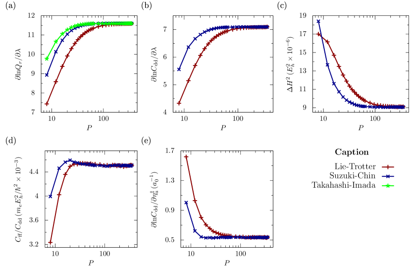
Figure 1: Convergence of various quantities required in the QI approximation of the KIE to the quantum limit as a function of the Trotter number $P$: (a) $\partial\mathrm{ln}Q_{r}/\partial\lambda$, (b) $\partial\mathrm{ln}C_{\text{dd}}/\partial\lambda$, (c) $\Delta H^{2}$, (d) $C_{\mathrm{ff}}/C_{\mathrm{dd}}$, (e) $\partial\mathrm{ln}C_{\text{dd}}/\partial\eta_{a}^{\ddagger}$. Results shown were obtained with the virial estimators and correspond to the KIE $\mathrm{\cdot H+H_{2}/\cdot D+D_{2}}$ at 200 K.

Statistical errors of different estimators are presented in Fig. 2. Note that they do not depend much on the factorization used. In contrast, the decrease of statistical errors associated with using virial estimators is remarkable for all quantities.

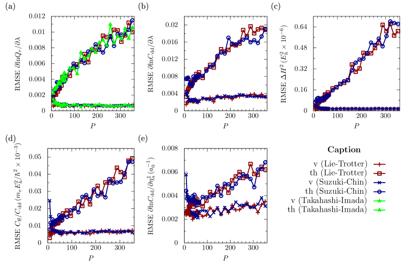
Figure 2: Statistical root mean square errors (RMSE) obtained with different estimators at different values of the Trotter number $P$ for quantities required in the QI approximation. (a) $\partial\mathrm{ln}Q_{r}/\partial\lambda$, (b) $\partial\mathrm{ln}C_{\text{dd}}/\partial\lambda$, (c) $\Delta H^{2}$, (d) $C_{\text{ff}}/C_{\text{dd}}$, (e) $\partial\mathrm{ln}C_{\text{dd}}/\partial\eta_{a}^{\ddagger}$. Results correspond to the KIE $\mathrm{\cdot H+H_{2}/\cdot D+D_{2}}$ at 200 K. “v” stands for “virial”, “th” - for “thermodynamic”.

To compare the speedups achieved by different combinations of splittings and estimators we estimated the relative CPU times needed to converge the quantities $\Delta H$, $C_{\mathrm{ff}}/C_{\mathrm{dd}}$, $Q_{r}^{(B)}/Q_{r}^{(A)}$, and $C_{\text{dd}}^{(B)}/C_{\text{dd}}^{(A)}$ to $1\%$ discretization and statistical errors. To estimate the speedup associated with calculating the overall KIE itself with $1\%$ statistical and discretization errors we ran a separate set of simulations with $\lambda=1$ in addition to those for $\lambda=0$; the statistical and discretization errors of the KIE calculated with different combinations of estimators and factorizations were then approximated with the corresponding errors obtained if thermodynamic integration of $Q_{r}$ and $C_{\mathrm{dd}}$ had been performed using a single step trapezoidal rule (i.e., based just on the two boundary points $\lambda=0$ and $\lambda=1$).

Let us assume the CPU time of a simulation to be approximately proportional to $P$ and the number of MC steps. Then for a given combination of factorization and estimator the cost of achieving the target discretization and statistical errors is proportional to the product $\tilde{P}\sigma_{\tilde{P}}^{2}$, where $\tilde{P}$ is the value of the Trotter number that yields the target discretization error and $\sigma_{\tilde{P}}$ is the statistical error exhibited by the estimator at this value of $P$. These estimates of CPU cost are then corrected by the increase in CPU time associated with using the fourth-order splittings and virial estimators. The final results are presented in Tab. IV.1.2, which confirms that the combination of virial estimators and fourth-order splittings leads to a significant speedup of the calculation.

One may be surprised that the value of $P$ necessary to achieve $1\%$ convergence of $C_{\mathrm{ff}}/C_{\mathrm{dd}}$ appears to be roughly independent of the splitting used; this is probably because the discretization errors of $C_{\mathrm{dd}}$ and $C_{\mathrm{ff}}$ cancel to a larger extent for the LT than the SC splitting. Taking the discretization error to be $0.5\%$ rather than $1\%$ makes the difference in the required value of $P$ even more pronounced: $P=40$ for the LT and $P=80$ for the SC splitting.

Note that even though the values of $P$ required to converge individual quantities are quite large (up to $P=336$ for $\partial\ln Q_{r}/\partial\lambda$ if LT splitting is used), the Trotter number $P$ necessary to converge the final KIE result is significantly lower due to the cancellation of discretization errors between individual quantities and especially between the two isotopologs. However, our $P$ value required for the KIE computed with the LT splitting is still larger than, for instance, those used in Ref. Yamamoto and Miller, 2004, where the authors obtained the final result by extrapolating to the $P\rightarrow\infty$ limit.

It is also interesting to relate our results to those of Ref. Engel et al., 2015, where the authors compared efficiencies of the LT, TI, and fourth-order ChinChin and Chen (2002); Chin (2004) factorizations for finding different quantities associated with the RPMD expression for the reaction rate. The authors found that for dynamical properties the TI splitting gives little improvement over the standard LT factorization, which is consistent with our explanation presented in Subsec. III.1; both factorizations are outperformed by the fourth-order Chin factorization, which is in agreement with the SC outperforming LT splitting in Tab. IV.1.2. For equilibrium properties, the authors found that the efficiencies of the Chin and TI factorizations are similar, and that both fourth-order factorizations significantly outperform the standard LT splitting, again in agreement with our results and explanation.

We mentioned earlier that we had calculated virial estimators by finite difference, making the computational cost of their evaluation independent of dimensionality. To employ fourth-order splittings, however, one must know the potential gradient for all $P$ replicas (for the TI splitting) or at least for $P/2$ replicas (for the SC splitting if $\alpha=0$ or $\alpha=1$). In general, if evaluating the gradient becomes too expensive compared to the potential energy itself, it may be advantageous to use the LT instead of the fourth-order splittings. For example, as shown in Tab. IV.1.2, using the fourth-order splittings decreased the necessary $P$ approximately four times; therefore, for this particular system it is reasonable to use the TI factorization if the cost of evaluating the gradient is smaller than three times the cost of evaluating the potential alone. For the SC factorization the corresponding factor is around six, since one needs only $P/2$ force evaluations. This upper bound for efficiency may be pushed further using the reweighting-based techniques;Jang, Jang, and Voth (2001); Yamamoto (2005); Pérez and Tuckerman (2011) this approach, however, is known to increase the statistical errors of the final result in high-dimensional systems.Ceriotti et al. (2012)

Table 2: Estimated speedups of the QI calculations achieved by the use of various combinations of path integral factorizations and estimators (th = thermodynamic, v = virial). Speedup “1” (i.e., no speedup) corresponds to the standard method employing a combination of the Lie-Trotter factorization and thermodynamic estimators. Results correspond to the KIE $\mathrm{\cdot H+H_{2}/\cdot D+D_{2}}$ at 200 K.

Factorization		Lie-Trotter (LT)				Suzuki-Chin (SC)				Takahashi-Imada (TI)
Estimator		$P$	th	v		$P$	th	v		$P$	th	v
$\partial\mathrm{ln}Q_{r}/\partial\lambda$		336	$1$	$220$		$96$	$10$	$850$		64	44	1200
$\partial\mathrm{ln}C_{\text{dd}}/\partial\lambda$		$240$	$1$	$19$		$64$	$13$	$160$		_	_	_
$\Delta H^{2}$		$128$	$1$	$170$		$48$	$14$	$380$		_	_	_
$C_{\text{ff}}/C_{\text{dd}}$		$36$	$1$	$2.7$		$32$	$1.3$	$3.0$		_	_	_
$\partial\mathrm{ln}C_{\text{dd}}/\partial\eta_{a}^{\ddagger}$		$80$	$1$	$1.7$		$16$	$3.6$	$3.8$		_	_	_
KIE		$128$	$1$	$34$		$40$	$12$	$97$		_	_	_

Lastly, we verified the modified methodology by comparing our result for the KIE $\mathrm{\cdot H+H_{2}/\cdot D+D_{2}}$ with those of Ref. Vaníček et al., 2005, obtained both with the QI approximation and with an exact quantum method. For each temperature we calculated $\Delta H$ and $C_{\text{ff}}/C_{\text{dd}}$ by PIMC simulations with $1.28\times 10^{8}$ steps at $\lambda=0$ and $\lambda=1$. Ratios of $Q_{r}$ and $C_{\text{dd}}$ were evaluated by rewriting them as in Eqs. (54) and (55) respectively and finding the integral over $\lambda$ using Simpson’s rule with integration step $\Delta\lambda=0.1$. At $T=200\ \text{K}$ we also ran calculations with $\Delta\lambda=0.05$ to verify that the integration error of the final result is lower than the statistical error. Values of $\partial\mathrm{ln}C_{\text{dd}}/\partial\lambda$ within the integration interval were obtained by running simulations with $6.4\times 10^{7}$ MC steps (i.e., fewer steps than for the $\lambda$-endpoint simulations because $\partial\mathrm{ln}C_{\text{dd}}/\partial\lambda$ and $\partial\mathrm{ln}Q_{r}/\partial\lambda$ tend to converge faster than $C_{\text{ff}}/C_{\text{dd}}$ and especially than $\Delta H$). These conditions ensured that the total relative error of the final KIE caused by statistical noise was below $1\%$. We chose $P$ in such a way that the relative error due to $P$ being finite was less than the statistical one. At the lowest temperature $T=200\,\text{K}$ we chose $P=64$, while for $T=2400\ \text{K}$ $P=12$ turned out to be appropriate; for other temperatures we estimated the necessary $P$ by interpolation assuming that the $1/P$ is a linear function of $T$. To verify that the chosen values of $P$ were sufficient we ran additional simulations at temperatures $200$ K, $1000$ K, and $2400$ K with $\lambda=0$ and $\lambda=1$ with a doubled value of $P$. If two KIE’s calculated with $\Delta\lambda=1$ at the two different values of $P$ differed by a value that was lower then the sum of their statistical errors, the lower value of $P$ was deemed sufficient for the calculation. The statistical errors, i.e., root mean square errors (RMSE) were estimated with the “block-averaging” methodFlyvbjerg and Petersen (1989) in order to remove the effect of correlation length of the random walk in the Metropolis MC simulation.

In Ref. Vaníček et al., 2005, $\eta_{\gamma}^{\ddagger}$ were taken to be $0$ for all temperatures and all values of $\lambda$. Even though this choice of DS positions leads to $C_{\mathrm{dd}}$ being stationary, it is a local minimum rather than a saddle point. We therefore also checked the result for the case when the proper optimal DS positions are found. Since from symmetry considerations the optimal DS parameters satisfy $\eta_{a}^{\ddagger}=-\eta_{b}^{\ddagger}$, simple bisection was sufficient to calculate the values up to $0.01$ a.u. The results are presented in Table IV.1.2. Intermediate results of the calculations are presented separately in Table V in Appendix C. We can see that the values obtained with $\eta_{\gamma}^{\ddagger}=0$ agree well with those of Ref. Vaníček et al., 2005, validating our modifications. It can also be seen that the full DS optimization improves agreement of the QI results with the exact quantum result, making the method remarkably accurate at low temperatures.

Table 3: Kinetic isotope effect $\mathrm{\cdot H+H_{2}/\cdot D+D_{2}}$ at different temperatures.

$T$ (K)	optimal $\eta^{\ddagger}_{a}=-\eta^{\ddagger}_{b}$		QI		QM	% error	QI
	$\lambda=0$	$\lambda=1$	no DS optimization	optimized DS
200	$1.00$	$0.41$	$22.3\pm 0.2$	$22.6\pm 0.3$	$22.53$	$<1$	$23.15$
250	$0.62$	$0$	$10.91\pm 0.08$	$9.92\pm 0.09$	$10.40$	$-5$	$10.98$
300	$0.01$	$0$	$7.38\pm 0.05$	$7.35\pm 0.05$	$6.97$	$5$	$7.41$
400	$0$	$0$	_	$4.87\pm 0.03$	$4.74$	$3$	$4.84$
600	$0$	$0$	_	$3.29\pm 0.02$	$3.42$	$-4$	$3.25$
1000	$0$	$0$	_	$2.23\pm 0.01$	$2.61$	$-15$	$2.22$
1500	$0$	$0$	_	$1.81\pm 0.01$	$2.27$	$-20$	$1.83$
2400	$0$	$0$	_	$1.55\pm 0.01$	_	_	$1.56$

IV.2 $\mathbf{CH_{4}+\cdot H\rightleftharpoons\cdot CH_{3}+H_{2}}$ exchange

As mentioned, the KIE’s on the $\mathrm{CH_{4}+\cdot H\rightleftharpoons\cdot CH_{3}+H_{2}}$ exchange had been studied by various numerical methods, but not by the QI approximation. We therefore decided to test the accelerated QI method on this reaction using the potential energy surface published in Ref. Zhang, Braams, and Bowman, 2006.

IV.2.1 Computational details

We first ran a series of trial simulations to roughly determine the value of $P$ and the number of MC steps ensuring that at the lowest temperature the relative statistical error of the KIE is below $1\%$ and that the discretization error with respect to $P$ is even smaller. The target statistical error was guaranteed by running $6.4\times 10^{7}$ step MC simulations at $\lambda=0$ and $\lambda=1$, and $3.2\times 10^{7}$ simulations at other values of $\lambda$. The target discretization error was achieved with $P=80$ for the LT and $P=20$ for the combination of fourth-order splittings at $T=400\,\textmd{K}$; at other temperatures $P$ was chosen such that the ratio $\beta/P$ stayed approximately constant. We chose $\Delta\lambda=0.1$ as for the case of $\mathrm{\cdot H+H_{2}/\cdot D+D_{2}}$; to be completely sure that the thermodynamic integration error was negligible to the statistical one, we also ran calculations with $\Delta\lambda=0.05$ at $T=400\mathrm{K}$ for the equilibrium isotope effect $\mathrm{\cdot CH_{3}/\cdot CD_{3}}$ and KIE $\mathrm{\cdot CH_{3}+D_{2}}/\mathrm{\cdot CD_{3}+D_{2}}$, as these cases exhibited the most drastic changes of properties during thermodynamic integration.

To determine the stationary positions of the DS’s ($\{\eta_{\gamma}^{\ddagger}\}$) we ran several short ($8\times 10^{6}$ steps) simulations to find the sign of $\partial\ln C_{\mathrm{dd}}/\partial\eta_{\gamma}^{\ddagger}$ at different DS positions; the saddle points were found with accuracy of $0.01$ a.u. The difference between $\eta_{a}^{\ddagger}$ and $\eta_{b}^{\ddagger}$ turned out to be negligible at all temperatures considered, in accordance with what is expected at “high” temperatures.Zhao, Yamamoto, and Miller (2004) The calculated values of $\eta^{\ddagger}$ are presented in Tab. 13 in Appendix C; as expected, they are quite close to the position of the classical transition state at $\eta^{\ddagger}=-0.94$.

IV.2.2 Results

Next, we compared results obtained by the accelerated method (employing a combination of fourth-order splittings and virial estimators) and by the standard method (employing a combination of LT splitting and thermodynamic estimators). The corresponding numerical results are labeled as “accel.” and “std.,” respectively. For further comparison, we calculated the same KIE’s also with the conventional transition state theory (TST)Eyring (1935); M. G. Evans (1935); Mahan (1974) and TST with Wigner tunneling correctionWigner (1932) (in the tables the corresponding columns are denoted as “TST” and “TST + Wigner” respectively). In the TST framework the expression for the rate constant takes the form

$$k_{\mathrm{TST}}=\frac{k_{\mathrm{B}}T}{h}\frac{Q^{\ddagger}}{Q_{r}},$$ (85)

where $Q^{\ddagger}$ and $Q_{r}$ are partition functions of the transition and reactant states, computed assuming separability of rotations and vibrations, harmonic approximation for vibrations, and rigid rotor approximation for rotations. Note that the usual factor $\exp(-E_{a}/k_{B}T)$, where $E_{a}$ is the activation energy, is absorbed into our definition of $Q^{\ddagger}$ since we use the same zero of energy for both $Q^{\ddagger}$ and $Q_{r}$. This expression can be multiplied by the so-called Wigner tunneling correction

$$\kappa=1+\frac{1}{24}(\hbar\beta|\omega^{\ddagger}|)^{2}$$ (86)

to account for tunneling contribution to the reaction rate. Here $\omega^{\ddagger}$ is the imaginary frequency corresponding to the motion along the reaction coordinate,

$$\omega^{\ddagger}=\sqrt{\frac{K^{\ddagger}}{\mu^{\ddagger}}},$$ (87)

$\mu^{\ddagger}$ is the effective reduced mass of the movement along the reaction coordinate at the saddle point, and $K^{\ddagger}$ is the corresponding negative force constant. Since the conventional TST expression captures the changes of zero point energy as well as of the rotational and translational partition functions due to the isotopic substitution, one may expect that the difference between the QI and conventional TST should be largely due to the difference between the extent of tunneling present in the two isotopologs. The results are presented in Tables 4-10.

Table 4: Kinetic isotope effect $\mathrm{CH_{4}+\cdot H}/\mathrm{CH_{4}+\cdot D}$.

$T$ (K)	TST	TST +Wigner	QI		TST	CVT/$\mathrm{\mu OMT}$	RDQD	RPMD	Expt.
			accel.	std.
400	0.56	0.56	0.60$\pm 0.01$	0.62$\pm 0.07$	0.54	0.58	0.64		0.74
500	0.66	0.66	0.70$\pm 0.01$	0.65$\pm 0.08$	0.65	0.67	1.03	0.65	0.84
600	0.74	0.74	0.78$\pm 0.01$	0.7$\pm 0.1$	0.73	0.74	1.23		0.91
700	0.79	0.79	0.84$\pm 0.01$	0.9$\pm 0.1$	0.78	0.79	1.33	0.80	0.97

Table 5: Kinetic isotope effect $\mathrm{\cdot CH_{3}+D_{2}}/\mathrm{\cdot CD_{3}+D_{2}}$.

$T$ (K)	TST	TST+Wigner	QI		TST	CVT/$\mathrm{\mu OMT}$	Expt.
			accel.	std.
400	0.73	0.74	0.76$\pm 0.01$	0.7$\pm 0.1$	0.75	0.74	0.59
500	0.82	0.82	0.83$\pm 0.01$	0.9$\pm 0.1$	0.83	0.82	0.72
600	0.87	0.88	0.88$\pm 0.01$	0.8$\pm 0.2$	0.88	0.88	0.82
700	0.91	0.91	0.90$\pm 0.01$	0.8$\pm 0.2$	0.92	0.91	0.90

Table 6: Kinetic isotope effect $\mathrm{\cdot CH_{3}+H_{2}}/\mathrm{\cdot CD_{3}+H_{2}}$.

$T$ (K)	TST	TST+Wigner	QI		TST	CVT/$\mathrm{\mu OMT}$	Expt.
			accel.	std.
400	0.74	0.74	0.80$\pm 0.01$	0.78$\pm 0.08$	0.75	0.81	0.85
500	0.82	0.83	0.86$\pm 0.01$	0.9$\pm 0.1$	0.83	0.88	0.86
600	0.87	0.88	0.90$\pm 0.01$	1.0$\pm 0.2$	0.88	0.92	0.87
700	0.91	0.91	0.92$\pm 0.01$	1.0$\pm 0.2$	0.92	0.95	0.88

Table 7: Kinetic isotope effect $\mathrm{\cdot CH_{3}+HD}/\mathrm{\cdot CH_{3}+DH}$.

$T$ (K)	TST	TST+Wigner	QI		TST	CVT/$\mathrm{\mu OMT}$	Expt.
			accel.	std.
467	1.51	1.86	2.10$\pm 0.02$	2.5$\pm 0.4$	1.50	1.83	2.1$\pm$0.5
531	1.48	1.76	1.84$\pm 0.02$	2.0$\pm 0.3$	1.47	1.71	1.9$\pm$0.3
650	1.44	1.64	1.59$\pm 0.02$	1.4$\pm 0.3$	1.43	1.56	1.2$\pm$0.3

Table 8: Kinetic isotope effect $\mathrm{\cdot CD_{3}+HD}/\mathrm{\cdot CD_{3}+DH}$.

$T$ (K)	TST	TST+Wigner	QI		TST	CVT/$\mathrm{\mu OMT}$	Expt.
			accel.	std.
400	1.56	1.99	2.52$\pm 0.02$	2.3$\pm 0.3$	1.55	1.91	1.85
500	1.50	1.80	1.95$\pm 0.02$	1.9$\pm 0.3$	1.49	1.60	1.61
600	1.46	1.68	1.65$\pm 0.02$	1.3$\pm 0.3$	1.45	1.56	1.47
700	1.43	1.60	1.52$\pm 0.01$	1.6$\pm 0.3$	1.42	1.49	1.38

Table 9: Kinetic isotope effect $\mathrm{\cdot CD_{3}+H_{2}}/\mathrm{\cdot CD_{3}+D_{2}}$.

$T$ (K)	TST	TST+Wigner	QI		TST	CVT/$\mathrm{\mu OMT}$	Expt.
			accel.	std.
400	3.45	4.39	5.60$\pm 0.04$	5.0$\pm 0.8$	3.22	4.13	3.33
500	2.98	3.57	3.92$\pm 0.03$	3.9$\pm 0.5$	2.83	3.21	2.88
600	2.64	3.04	3.15$\pm 0.03$	2.6$\pm 0.6$	2.54	2.73	2.61
700	2.40	2.68	2.75$\pm 0.02$	2.5$\pm 0.4$	2.33	2.43	2.43

Table 10: Kinetic isotope effect $\mathrm{\cdot CH_{3}+H_{2}}/\mathrm{\cdot CH_{3}+D_{2}}$.

$T$ (K)	TST	TST+Wigner	QI		TST	CVT/$\mathrm{\mu OMT}$	Expt.
			accel.	std.
400	3.45	4.41	5.93$\pm 0.05$	5.8$\pm 0.8$	3.22	4.57	4.8$\pm$0.4
500	2.97	3.58	4.09$\pm 0.04$	4.0$\pm 0.6$	2.83	3.43	3.5$\pm$0.2
600	2.64	3.05	3.21$\pm 0.03$	3.1$\pm 0.5$	2.54	2.86	2.8$\pm$0.2

First of all, it can be seen that for KIE’s due to mass changes not affecting the transferred atom (see Tables 4-6) the QI values are close to those obtained by conventional TST. This can be understood qualitatively from the expression (86) for Wigner tunneling correction for reaction rates. The main contribution to $\mu^{\ddagger}$ appearing in the expression for $\omega^{\ddagger}$ comes from the transferred atom, therefore if its mass does not change, the Wigner tunneling corrections for different isotopologs will have similar values and largely cancel out in the KIE.

Second, note that, in agreement with the usual difference in magnitudes of secondary and primary isotope effects, replacing $\mathrm{\cdot CH_{3}}$ with $\mathrm{\cdot CD_{3}}$ leads to a much smaller rate change than does replacing $\mathrm{H_{2}}$ with $\mathrm{D_{2}}$ (compare Tables 5-6 and 9-10) This consideration also explains why the KIE’s corresponding to $\mathrm{\cdot CH_{3}+H_{2}}/\mathrm{\cdot CH_{3}+D_{2}}$ and $\mathrm{\cdot CD_{3}+H_{2}}/\mathrm{\cdot CD_{3}+D_{2}}$ are quite close to each other (see Tables 10 and 9). For some KIE’s presented in Tables 8-10 it appears that results obtained with TST or TST with Wigner tunneling correction are in better agreement with experimental values than those obtained with the QI, probably indicating that a large cancellation takes place between the errors of the TST and of the potential energy surface (PES).

In order to estimate the influence of the used force field on the final result we also ran calculations with the PES published in Ref. Corchado, Bravo, and Espinosa-Garcia, 2009 for $\mathrm{CH_{4}+\cdot H/CH_{4}+\cdot D}$. After finding the optimal DS positions (see Table 13 in Appendix C), we compared the QI values of this KIE obtained with the two PES’s from Refs. Corchado, Bravo, and Espinosa-Garcia, 2009 and Zhang, Braams, and Bowman, 2006 (see Table 11), finding that the choice of the PES affects the KIE value by as much as $10\%$. In contrast, comparison of the KIE’s computed with the same PES, but with two different accurate quantum methodologies (RPMD and QI) results in a remarkable agreement, within the statistical error of less than $2\%$. Finally, note that the QI KIE is in much better agreement with experiment if computed with the PES of Ref. Zhang, Braams, and Bowman, 2006 than with the PES of Ref. Corchado, Bravo, and Espinosa-Garcia, 2009, suggesting that the former PES, which was used for most of the calculations in this paper, was the appropriate choice.

Table 11: Influence of the potential energy surface (PES) on the KIE $\mathrm{CH_{4}+\cdot H}/\mathrm{CH_{4}+\cdot D}$. Comparison of the QI KIE’s calculated using the PES’s of Refs. Corchado, Bravo, and Espinosa-Garcia, 2009 and Zhang, Braams, and Bowman, 2006. Note also the remarkable agreement between the KIE’s computed with RPMD and QI on the same PES.

$T$ (K)	PES of Ref. Corchado, Bravo, and Espinosa-Garcia,2009				PES of Ref. Zhang, Braams, and Bowman,2006	Expt.
	TST	TST+Wigner	RPMD	QI	QI
400	0.52	0.52		0.54$\pm 0.01$	0.60$\pm 0.01$	0.74
500	0.63	0.63	0.65	0.64$\pm 0.01$	0.70$\pm 0.01$	0.84
600	0.71	0.71		0.73$\pm 0.01$	0.78$\pm 0.01$	0.91
700	0.77	0.77	0.80	0.79$\pm 0.01$	0.84$\pm 0.01$	0.97

As for the performance of the fourth-order splittings, since an analytical gradient was not available for the $\mathrm{CH}_{4}+\cdot\mathrm{H}$ system, the gradient had to be calculated numerically using finite differences. For constrained simulations this made the force twelve times (once per each internal degree of freedom) as expensive as the potential itself, leading to a seven-fold increase in CPU time for a given $P$ and number of MC steps when the SC splitting was used. Since the fourth-order splitting decreased the necessary $P$ by a factor of four, the final increase in CPU time for a given discretization error and number of MC steps was $75\%$. For unconstrained simulations employed to find $\cdot\mathrm{CH}_{3}/\cdot\mathrm{CD}_{3}$ equilibrium isotope effect the force was six times as expensive as the potential; since the use of the TI factorization allowed to decrease $P$ four times, the final increase in CPU time was also $75\%$ for a given number of MC steps and discretization error.

In summary, the KIE’s were reproduced in a reasonable agreement with experiment. The differences are probably due to both the error of the potential energy surface used and the large experimental error. Note that our accelerated methodology again drastically reduced both the discretization and statistical errors of the calculations.

V Conclusions

In conclusion, we have accelerated the methodology from Ref. Vaníček et al., 2005 for computing KIE’s with the QI approximation. In particular, we have combined virial estimators (several of which have been derived for the first time here) with high-order factorizations of the quantum Boltzmann operator, and shown that this combination significantly accelerates the QI calculations of the KIE’s in systems with prominent quantum effects. We have also proposed and demonstrated the utility of a new method for the thermodynamic integration of the delta-delta correlation function $C_{\text{dd}}$, which is a convenient alternative to the approach employed in Ref. Vaníček et al., 2005. Our accelerated methodology has been tested on the $\mathrm{CH_{4}+\cdot H\rightleftharpoons\cdot CH_{3}+H_{2}}$ model exchange, obtaining results that agree reasonably well with published experimental values.

Appendix A: derivation of the fourth-order corrections for different estimators

When one of the fourth-order factorizations is used, $V_{\mathrm{eff}}^{(s)}(\mathbf{r}^{(s)})$ has an explicit dependence on mass and $\beta$; as a result one needs to add appropriate “corrections” to the estimators arising from the differentiation with respect to these quantities.

For $\partial\mathrm{ln}Q_{r}/\partial\lambda/\beta$ and $\partial\mathrm{ln}C_{\mathrm{dd}}/\partial\lambda/\beta$, it follows from Eqs. (57) and (58) that the correction $F_{r,\mathrm{grad}}$ is

$$F_{r,\mathrm{grad}}=-\frac{\beta}{P^{3}}\sum_{i=1}^{N}\frac{\mathit{d}m_{i}}{\mathit{d}\lambda}\sum_{s=1}^{P}w_{s}d_{s}\frac{\partial V_{\mathrm{grad}}(\mathbf{r}^{(s)})}{\partial m_{i}}=\frac{\hbar^{2}\beta}{P^{3}}\sum_{s=1}^{P}w_{s}d_{s}\sum_{i=1}^{N}\frac{1}{m_{i}^{2}}\frac{\mathit{d}m_{i}}{\mathit{d}\lambda}|\nabla_{i}V(\mathbf{r}^{(s)})|^{2}.$$ (88)

Note that when a coordinate rescaling is used to obtain an estimator (e.g., for centroid virial estimators), the correction remains the same due to the following equality:

$$\frac{\mathit{d}V_{\mathrm{eff}}^{(s)}[\mathbf{r}^{(s)}(m_{i}),m_{i}]}{\mathit{d}m_{i}}=\left\langle\frac{\partial\mathbf{r}^{(s)}}{\partial m_{i}},\frac{\partial V_{\mathrm{eff}}^{(s)}}{\partial\mathbf{r}^{(s)}}\right\rangle_{0}+d_{s}\left(\frac{\beta}{P}\right)^{2}\frac{\partial V_{\mathrm{grad}}}{\partial m_{i}}.$$ (89)

As for $F_{\mathrm{th}}$ and $F_{\mathrm{v}}$, since

$$\frac{\partial V_{\mathrm{eff}}^{(s)}(\mathbf{r}^{(s)})}{\partial\beta}=2d_{s}\frac{\beta}{P^{2}}V_{\mathrm{grad}}(\mathbf{r}^{(s)})\text{,}$$ (90)

the gradient correction to be added is

$$F_{\mathrm{grad}}=\frac{4\beta^{2}}{P^{3}}\left(\sum_{s=1}^{P/2-1}-\sum_{s=P/2+1}^{P-1}\right)w_{s}d_{s}V_{\mathrm{grad}}(\mathbf{r}^{(s)})\text{.}$$ (91)

Again, this correction is the same for the virial and thermodynamic variants.

Since the $G$ factor involves the second derivatives with respect to $\beta$, the corrections will be different for $G_{\mathrm{th}}$ and $G_{\mathrm{v}}$. While $G_{\mathrm{th,grad}}$ is obtained easily as

$$G_{\mathrm{th,grad}}=-\frac{24\beta}{P^{3}}\sum_{s=1}^{P}w_{s}d_{s}V_{\mathrm{grad}}(\mathbf{r}^{(s)}),$$ (92)

to find $G_{\mathrm{v}}$, one needs to take advantage of the following relations:

$$\frac{\mathit{d}V_{\mathrm{eff}}^{(s)}[\mathbf{r}^{(s)}(\beta),\beta]}{\mathit{d}\beta}=\left\langle\frac{\partial\mathbf{r}^{(s)}(\beta)}{\partial\beta},\frac{\partial V_{\mathrm{eff}}^{(s)}(\mathbf{r}^{(s)})}{\partial\mathbf{r}^{(s)}}\right\rangle_{0}+\frac{\partial V_{\mathrm{eff}}^{(s)}(\mathbf{r}^{(s)})}{\partial\beta}\text{,}$$ (93)

$$\begin{split}\frac{\mathit{d}^{2}V^{(s)}_{\mathrm{eff}}[\mathbf{r}^{(s)}(\beta),\beta]}{\mathit{d}\beta^{2}}=&\left\langle\frac{\partial^{2}\mathbf{r}^{(s)}(\beta)}{\partial\beta^{2}},\frac{\partial V^{(s)}_{\mathrm{eff}}(\mathbf{r}^{(s)})}{\partial\mathbf{r}^{(s)}}\right\rangle_{0}+\left\langle\frac{\partial\mathbf{r}^{(s)}(\beta)}{\partial\beta},\frac{\partial^{2}V^{(s)}_{\mathrm{eff}}(\mathbf{r}^{(s)})}{(\partial\mathbf{r}^{(s)})^{2}},\frac{\partial\mathbf{r}^{(s)}(\beta)}{\partial\beta}\right\rangle_{00}\\ &+2\left\langle\frac{\partial\mathbf{r}^{(s)}(\beta)}{\partial\beta},\frac{\partial}{\partial\mathbf{r}^{(s)}}\left[\frac{\partial V^{(s)}_{\mathrm{eff}}(\mathbf{r}^{(s)})}{\partial\beta}\right]\right\rangle_{0}+\frac{\partial^{2}V^{(s)}_{\mathrm{eff}}(\mathbf{r}^{(s)})}{\partial\beta^{2}}\text{,}\end{split}$$ (94)

$$\begin{split}\frac{\mathit{d}^{2}\{\beta V^{(s)}_{\mathrm{eff}}[\mathbf{r}^{(s)}(\beta),\beta]\}}{\mathit{d}\beta^{2}}=&2\frac{\mathit{d}V^{(s)}_{\mathrm{eff}}(\mathbf{r}^{(s)})}{\mathit{d}\beta}+\beta\frac{\mathit{d}^{2}V^{(s)}_{\mathrm{eff}}(\mathbf{r}^{(s)})}{\mathit{d}\beta^{2}}\\ =&\left\langle\left(2\frac{\partial\mathbf{r}^{(s)}(\beta)}{\partial\beta}+\beta\frac{\partial^{2}\mathbf{r}^{(s)}(\beta)}{\partial\beta^{2}}\right),\frac{\partial V^{(s)}_{\mathrm{eff}}(\mathbf{r}^{(s)})}{\partial\mathbf{r}^{(s)}}\right\rangle_{0}\\ &+\beta\left\langle\frac{\partial\mathbf{r}^{(s)}(\beta)}{\partial\beta},\frac{\partial^{2}V^{(s)}_{\mathrm{eff}}(\mathbf{r}^{(s)})}{(\partial\mathbf{r}^{(s)})^{2}},\frac{\partial\mathbf{r}^{(s)}(\beta)}{\partial\beta}\right\rangle_{00}\\ &+2\beta\left\langle\frac{\partial\mathbf{r}^{(s)}(\beta)}{\partial\beta},\frac{\partial}{\partial\mathbf{r}^{(s)}(\beta)}\left[\frac{\partial V^{(s)}_{\mathrm{eff}}(\mathbf{r}^{(s)})}{\partial\beta}\right]\right\rangle_{0}+\beta\frac{\partial^{2}V^{(s)}_{\mathrm{eff}}(\mathbf{r}^{(s)})}{\partial\beta^{2}}+2\frac{\partial V^{(s)}_{\mathrm{eff}}(\mathbf{r}^{(s)})}{\partial\beta}\text{,}\end{split}$$ (95)

The only terms for which the explicit $\beta$ dependence plays a role are the last three. As a result we get:

$$\begin{split}G_{\mathrm{v,grad}}&=-\frac{4}{P}\sum_{s=1}^{P}w_{s}\left\{2\beta\left\langle\frac{\partial\mathbf{r}^{(s)}(\beta)}{\partial\beta},\frac{\partial}{\partial\mathbf{r}^{(s)}(\beta)}\left[\frac{\partial V^{(s)}_{\mathrm{eff}}(\mathbf{r}^{(s)})}{\partial\beta}\right]\right\rangle_{0}+\beta\frac{\partial^{2}V^{(s)}_{\mathrm{eff}}(\mathbf{r}^{(s)})}{\partial\beta^{2}}+2\frac{\partial V^{(s)}_{\mathrm{eff}}(\mathbf{r}^{(s)})}{\partial\beta}\right\}\text{.}\end{split}$$ (96)

This expression can be rewritten as

$$G_{\mathrm{v,grad}}=-\frac{8\beta}{P^{3}}\sum_{s=1}^{P}w_{s}d_{s}\left[3V_{\mathrm{grad}}\vphantom{(\mathbf{r}^{(s)}-\check{\mathbf{r}}^{(s)})}\right.\left.+\left\langle(\mathbf{r}^{(s)}-\check{\mathbf{r}}^{(s)}),\nabla V_{\mathrm{grad}}(\mathbf{r}^{(s)})\right\rangle_{0}\right].$$ (97)

Appendix B: derivation of $\mathbf{{B^{k(\gamma)}}}$

The present derivation is a slight generalization of the one found in Ref. den Otter, 2000. We start by transforming to mass-scaled coordinates,

$$\begin{split}\mathrm{x}_{i}^{(s)}&:=\sqrt{m_{i}}\mathrm{r}_{i}^{(s)},\\ \mathrm{x}_{\gamma i}&:=\sqrt{m_{i}}\mathrm{r}_{\gamma i},\\ \overline{\xi}_{\gamma}(\mathbf{x}_{\gamma})&:=\xi_{\gamma}(\mathbf{r}_{\gamma}),\end{split}$$ (98)

which will simplify the subsequent algebra due to the equality

$$||\nabla\xi_{\gamma}(\mathbf{r}_{\gamma})||_{-}=|\nabla\overline{\xi}_{\gamma}(\mathbf{x}_{\gamma})|.$$ (99)

In mass-scaled coordinates, the PI representation (29) of the delta-delta correlation function can be rewritten as

$$C_{\text{dd},P}=\int\overline{\rho}(\{\mathbf{x}^{(s)}\})\Delta[\overline{\xi}_{\gamma}(\mathbf{x}_{\gamma})]\mathit{d}\{\mathbf{x}^{(s)}\},$$ (100)

where the second normalized delta function has been absorbed into $\overline{\rho}$ in order to simplify the following derivation. Differentiation of $C_{\text{dd},P}$ with respect to the DS’s parameters yields

$$\begin{split}\frac{\partial C_{\text{dd},P}}{\partial\eta_{k}^{(\gamma)}}=&\frac{\partial}{\partial\eta_{k}^{(\gamma)}}\int\overline{\rho}(\{\mathbf{x}^{(s)}\})\Delta\left[\overline{\xi}_{\gamma}(\mathbf{x}_{\gamma},\eta_{k}^{(\gamma)})\right]\mathit{d}\{\mathbf{x}^{(s)}\}\\ =&\int\frac{\langle\nabla\overline{\xi}_{\gamma}(\mathbf{x}_{\gamma}),\nabla\overline{\xi}_{\gamma}(\mathbf{x}_{\gamma})\rangle}{|\nabla\overline{\xi}_{\gamma}(\mathbf{x}_{\gamma})|}\overline{\rho}(\{\mathbf{x}^{(s)}\})\frac{\partial\overline{\xi}_{\gamma}(\mathbf{x}_{\gamma})}{\partial\eta_{k}^{(\gamma)}}\frac{\mathit{d}}{\mathit{d}\overline{\xi}_{\gamma}}\left\{\delta\left[\overline{\xi}_{\gamma}(\mathbf{x}_{\gamma},\eta_{k}^{(\gamma)})\right]\right\}\mathit{d}\{\mathbf{x}^{(s)}\}\\ &+\int\frac{\partial\mathrm{ln}|\nabla\overline{\xi}_{\gamma}(\mathbf{x}_{\gamma})|}{\partial\eta_{k}^{(\gamma)}}\overline{\rho}(\{\mathbf{x}^{(s)}\})\Delta\left[\overline{\xi}_{\gamma}(\mathbf{x}_{\gamma},\eta_{k}^{(\gamma)})\right]\mathit{d}\{\mathbf{x}^{(s)}\}\\ =&\int\nabla\left\{\delta\left[\overline{\xi}_{\gamma}(\mathbf{x}_{\gamma},\eta_{k}^{(\gamma)})\right]\right\}\frac{\partial\overline{\xi}_{\gamma}(\mathbf{x}_{\gamma})}{\partial\eta_{k}^{(\gamma)}}\frac{\nabla\overline{\xi}_{\gamma}(\mathbf{x}_{\gamma})}{\left|\nabla\overline{\xi}_{\gamma}(\mathbf{x}_{\gamma})\right|}\overline{\rho}(\{\mathbf{x}^{(s)}\})\mathit{d}\{\mathbf{x}^{(s)}\}\\ &+\int\frac{1}{|\nabla\overline{\xi}_{\gamma}(\mathbf{x}_{\gamma})|^{2}}\left\langle\nabla\overline{\xi}_{\gamma},\nabla\frac{\partial\overline{\xi}_{\gamma}(\mathbf{x}_{\gamma})}{\partial\eta_{k}^{(\gamma)}}\right\rangle\overline{\rho}(\{\mathbf{x}^{(s)}\})\Delta\left[\overline{\xi}_{\gamma}(\mathbf{x}_{\gamma},\eta_{k}^{(\gamma)})\right]\mathit{d}\{\mathbf{x}^{(s)}\}.\end{split}$$ (101)

After integrating by parts with respect to $\mathbf{x}_{\gamma}$ in the first integral, we get

$$\begin{split}\frac{\partial}{\partial\eta_{k}^{(\gamma)}}\int\overline{\rho}(\{\mathbf{x}^{(s)}\})\Delta\left[\overline{\xi}_{\gamma}(\mathbf{x}_{\gamma},\eta_{k}^{(\gamma)})\right]\mathit{d}\{\mathbf{x}^{(s)}\}=&-\int\frac{\partial\overline{\xi}_{\gamma}(\mathbf{x}_{\gamma})}{\partial\eta_{k}^{(\gamma)}}\left[\left\langle\nabla\overline{\xi}_{\gamma}(\mathbf{x}_{\gamma}),\nabla^{(\gamma)}\mathrm{ln}\overline{\rho}(\{\mathbf{x}^{(s)}\})\right\rangle_{0}\vphantom{\left\langle\nabla,\frac{\nabla\overline{\xi}_{\gamma}(\mathbf{x}_{\gamma})}{|\nabla\overline{\xi}_{\gamma}(\mathbf{x}_{\gamma})|}\right\rangle_{0}}\right.\\ &\left.+|\nabla\overline{\xi}_{\gamma}(\mathbf{x}_{\gamma})|\left\langle\nabla,\frac{\nabla\overline{\xi}_{\gamma}(\mathbf{x}_{\gamma})}{|\nabla\overline{\xi}_{\gamma}(\mathbf{x}_{\gamma})|}\right\rangle_{0}\right]/|\nabla\overline{\xi}_{\gamma}(\mathbf{x}_{\gamma})|^{2}\\ &\times\Delta\left[\overline{\xi}_{\gamma}(\mathbf{x}_{\gamma},\eta_{k}^{(\gamma)})\right]\overline{\rho}(\{\mathbf{x}^{(s)}\})\mathit{d}\{\mathbf{x}^{(s)}\}\text{.}\end{split}$$ (102)

Equation (62) is obtained by substituting the explicit expression for $\overline{\rho}$ and transforming back to Cartesian coordinates.

Appendix C: Additional numerical results

In this section we present some additional numerical results that were moved from the main text for the sake of clarity. Figure 3 depicts the logarithmic plots of the discretization errors of various ingredients of the QI approximation as functions of the Trotter number $P$. The discretization error for a quantity $A$ is defined as $|A_{P}-A_{\infty}|$, where $A_{\infty}$ was estimated by averaging $A_{P}$ over several highest values of $P$, for which the discretization error was considered negligible. The averaging was performed in order to reduce the statistical error. The plots in Fig. 3 demonstrate the faster convergence to the quantum limit achieved with higher-order factorizations: indeed, especially for the  logarithmic derivative of $Q_{r}$, one can see that the discretization error dependence approaches the asymptotic behavior $\mathcal{O}(P^{-2})$ for the LT and $\mathcal{O}(P^{-4})$ for the SC and TI factorizations. In addition, in all panels, it is clear for which value of $P$ the discretization error becomes smaller than the statistical error, since for higher values of $P$ the smooth dependence of the discretization error on $P$ is obscured by statistical noise.

Table V contains values of various factors used to obtain the results in Table IV.1.2 for the QI KIE on the reaction $\mathrm{\cdot H_{\alpha}+H_{\beta}H_{\gamma}\rightarrow H_{\alpha}H_{\beta}+\cdot H_{\gamma}}$ with optimized DS. Finally, Table 13 contains optimized DS positions that were used for calculating KIE’s on the $\mathrm{CH_{4}+\cdot H\rightleftharpoons\cdot CH_{3}+H_{2}}$.

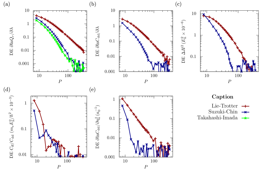
Figure 3: Absolute discretization error (DE) of different quantities as a function of $P$: (a) $\partial\mathrm{ln}Q_{r}/\partial\lambda$, (b) $\partial\mathrm{ln}C_{\text{dd}}/\partial\lambda$, (c) $\Delta H^{2}$, (d) $C_{\mathrm{ff}}/C_{\mathrm{dd}}$, (e) $\partial\mathrm{ln}C_{\text{dd}}/\partial\eta_{a}^{\ddagger}$. Results shown were obtained with the virial estimators and correspond to the KIE $\mathrm{\cdot H+H_{2}/\cdot D+D_{2}}$ at 200 K.

Table 12: Values of the factors entering the QI expression (52) for the KIE $\mathrm{\cdot H+H_{2}/\cdot D+D_{2}}$ with optimized dividing surface positions, displayed in Table IV.1.2. All quantities as well as their statistical errors are in atomic units.

$T$ (K)	$\Delta H^{2}\times 10^{6}$		$C_{\mathrm{ff}}/C_{\mathrm{dd}}\times 10^{3}$		$C_{\mathrm{dd}}$ ratio	$Q_{r}$ ratio
	$\lambda=0$	$\lambda=1$	$\lambda=0$	$\lambda=1$
200	$3.68\pm 0.03$	$4.27\pm 0.02$	$1.33\pm 0.01$	$2.03\pm 0.01$	$43.8\pm 0.3$	$1404\pm 1$
250	$4.87\pm 0.04$	$4.95\pm 0.03$	$2.01\pm 0.01$	$2.10\pm 0.01$	$55.8\pm 0.3$	$572.9\pm 0.3$
300	$7.40\pm 0.04$	$5.10\pm 0.03$	$2.73\pm 0.01$	$1.97\pm 0.01$	$49.5\pm 0.1$	$316.1\pm 0.2$
400	$7.92\pm 0.05$	$6.27\pm 0.04$	$2.49\pm 0.01$	$2.01\pm 0.01$	$33.96\pm 0.06$	$149.5\pm 0.1$
600	$12.0\pm 0.1$	$10.7\pm 0.1$	$2.77\pm 0.01$	$2.44\pm 0.01$	$23.11\pm 0.04$	$70.92\pm 0.03$
1000	$26.8\pm 0.1$	$24.5\pm 0.1$	$3.82\pm 0.03$	$3.55\pm 0.02$	$18.15\pm 0.02$	$39.42\pm 0.01$
1500	$54.3\pm 0.2$	$50.3\pm 0.2$	$5.29\pm 0.04$	$5.05\pm 0.02$	$16.78\pm 0.02$	$30.11\pm 0.01$
2400	$124.6\pm 0.4$	$117.1\pm 0.4$	$7.98\pm 0.05$	$7.80\pm 0.03$	$16.36\pm 0.01$	$25.51\pm 0.01$

Table 13: Optimal positions of the dividing surfaces along the reaction coordinate [see Eq. (83)] for transition states of several isotopic variants of the $\mathrm{CH_{4}+\cdot H}\rightleftharpoons\mathrm{\cdot CH_{3}+H_{2}}$ exchange at several temperatures.

Potential energy surface of Ref. Zhang, Braams, and Bowman,2006
TS	400 K	500 K	600 K	700 K
$\mathrm{H_{3}C\cdot\cdot\cdot H\cdot\cdot\cdot H}$	-0.91	-0.90	-0.88	-0.86
$\mathrm{H_{3}C\cdot\cdot\cdot H\cdot\cdot\cdot D}$	-0.88	-0.87	-0.85	-0.84
$\mathrm{D_{3}C\cdot\cdot\cdot H\cdot\cdot\cdot D}$	-0.89	-0.88	-0.86	-0.85
$\mathrm{D_{3}C\cdot\cdot\cdot D\cdot\cdot\cdot H}$	-0.93	-0.91	-0.89	-0.86
$\mathrm{H_{3}C\cdot\cdot\cdot D\cdot\cdot\cdot D}$	-0.89	-0.87	-0.86	-0.85
$\mathrm{D_{3}C\cdot\cdot\cdot D\cdot\cdot\cdot D}$	-0.90	-0.89	-0.87	-0.85
$\mathrm{D_{3}C\cdot\cdot\cdot H\cdot\cdot\cdot H}$	-0.92	-0.90	-0.89	-0.87
	467 K	531 K	650 K
$\mathrm{H_{3}C\cdot\cdot\cdot H\cdot\cdot\cdot D}$	-0.87	-0.86	-0.84
$\mathrm{H_{3}C\cdot\cdot\cdot D\cdot\cdot\cdot H}$	-0.90	-0.89	-0.87
Potential energy surface of Ref. Corchado, Bravo, and Espinosa-Garcia,2009
TS	400 K	500 K	600 K	700 K
$\mathrm{H_{3}C\cdot\cdot\cdot H\cdot\cdot\cdot H}$	-1.03	-1.00	-0.97	-0.95
$\mathrm{H_{3}C\cdot\cdot\cdot H\cdot\cdot\cdot D}$	-1.00	-0.97	-0.94	-0.92

References

- Sen and Kohen (2010) A. Sen and A. Kohen, J. Phys. Org. Chem 23, 613 (2010).
- Ramazani (2013) S. Ramazani, J. Chem. Phys. 138, 194305 (2013).
- Olsson, Siegbahn, and Warshel (2004) M. H. M. Olsson, P. E. M. Siegbahn, and A. Warshel, J. Am. Chem. Soc. 126, 2820 (2004).
- Banks and Clary (2007) S. T. Banks and D. C. Clary, Phys. Chem. Chem. Phys. 9, 933 (2007).
- Allen et al. (2013) J. W. Allen, W. H. Green, Y. Li, H. Guo, and Y. V. Suleimanov, J. Chem. Phys. 138, 221103 (2013).
- Hansen and Andersen (1994) N. F. Hansen and H. C. Andersen, J. Chem. Phys. 101, 6032 (1994).
- Pollak (2012) E. Pollak, J. Phys. Chem. B 116, 12966 (2012).
- Miller et al. (2003) W. H. Miller, Y. Zhao, M. Ceotto, and S. Yang, J. Chem. Phys. 119, 1329 (2003).
- Miller (1974) W. H. Miller, J. Chem. Phys. 61, 1823 (1974).
- Chapman, Garrett, and Miller (1975) S. Chapman, B. C. Garrett, and W. H. Miller, J. Chem. Phys. 63, 2710 (1975).
- Miller, Schwartz, and Tromp (1983) W. H. Miller, S. D. Schwartz, and J. W. Tromp, J. Chem. Phys. 79, 4889 (1983).
- Ceotto (2012) M. Ceotto, Mol. Phys. 110, 547 (2012).
- Zhao, Yamamoto, and Miller (2004) Y. Zhao, T. Yamamoto, and W. H. Miller, J. Chem. Phys. 120, 3100 (2004).
- Ceotto and Miller (2004) M. Ceotto and W. H. Miller, J. Chem. Phys. 120, 6356 (2004).
- Wang, Feng, and Zhao (2007) W. Wang, S. Feng, and Y. Zhao, J. Chem. Phys. 126, 114307 (2007).
- Wang and Zhao (2009) W. Wang and Y. Zhao, J. Chem. Phys. 130, 114708 (2009).
- Wang and Zhao (2011) W. Wang and Y. Zhao, Phys. Chem. Chem. Phys. 13, 19362 (2011).
- Wang and Zhao (2012) W. Wang and Y. Zhao, J. Chem. Phys. 137, 214306 (2012).
- Yamamoto and Miller (2004) T. Yamamoto and W. H. Miller, J. Chem. Phys. 120, 3086 (2004).
- Vaníček et al. (2005) J. Vaníček, W. H. Miller, J. F. Castillo, and F. J. Aoiz, J. Chem. Phys. 123, 054108 (2005).
- Jang, Jang, and Voth (2001) S. Jang, S. Jang, and G. A. Voth, J. Chem. Phys. 115, 7832 (2001).
- Yamamoto (2005) T. Yamamoto, J. Chem. Phys. 123, 104101 (2005).
- Pérez and Tuckerman (2011) A. Pérez and M. E. Tuckerman, J. Chem. Phys. 135, 064104 (2011).
- Buchowiecki and Vaníček (2013) M. Buchowiecki and J. Vaníček, Chem. Phys. Lett. 588, 11 (2013).
- Marsalek et al. (2014) O. Marsalek, P.-Y. Chen, R. Dupuis, M. Benoit, M. Méheut, Z. Bačić, and M. E. Tuckerman, J. Chem. Theory Comput. 10, 1440 (2014).
- Engel et al. (2015) H. Engel, R. Eitan, A. Azuri, and D. T. Major, Chem. Phys. 450-451, 95 (2015).
- Yang, Yamamoto, and Miller (2006) S. Yang, T. Yamamoto, and W. H. Miller, J. Chem. Phys. 124, 084102 (2006).
- Vaníček and Miller (2007) J. Vaníček and W. H. Miller, J. Chem. Phys. 127, 114309 (2007).
- Pu and Truhlar (2002) J. Pu and D. G. Truhlar, J. Chem. Phys. 117, 10675 (2002).
- Schatz, Wagner, and Dunning (1984) G. C. Schatz, A. F. Wagner, and T. H. Dunning, Jr., J. Phys. Chem. 88, 221 (1984).
- Kerkeni and Clary (2004) B. Kerkeni and D. C. Clary, J. Phys. Chem. A 108, 8966 (2004).
- Li et al. (2013) Y. Li, Y. V. Suleimanov, J. Li, W. H. Green, and H. Guo, J. Chem. Phys. 138, 094307 (2013).
- (33) M. Ceotto and W. H. Miller, private communication.
- Feynman and Hibbs (1965) R. P. Feynman and A. R. Hibbs, Quantum mechanics and path integrals (McGraw-Hill, 1965).
- Chandler and Wolynes (1981) D. Chandler and P. G. Wolynes, J. Chem. Phys. 74, 4078 (1981).
- Takahashi and Imada (1984) M. Takahashi and M. Imada, J. Phys. Soc. Jpn. 53, 963 (1984).
- Chin (1997) S. A. Chin, Phys. Lett. A 226, 344 (1997).
- Suzuki (1995) M. Suzuki, Physics Letters A 201, 425 (1995).
- Zimmermann and Vaníček (2009) T. Zimmermann and J. Vaníček, J. Chem. Phys. 131, 024111 (2009).
- Perez and von Lilienfeld (2011) A. Perez and O. A. von Lilienfeld, J. Chem. Theory Comput. 7, 2358 (2011).
- Ceriotti and Markland (2013) M. Ceriotti and T. E. Markland, J. Chem. Phys. 138, 014112 (2013), 10.1063/1.4772676.
- Cheng and Ceriotti (2014) B. Cheng and M. Ceriotti, J. Chem. Phys. 141, 244112 (2014).
- Herman, Bruskin, and Berne (1982) M. F. Herman, E. J. Bruskin, and B. J. Berne, J. Chem. Phys. 76, 5150 (1982).
- Parrinello and Rahman (1984) M. Parrinello and A. Rahman, J. Chem. Phys. 80, 860 (1984).
- Predescu and Doll (2002) C. Predescu and J. D. Doll, J. Chem. Phys. 117, 7448 (2002).
- Sprik, Klein, and Chandler (1985a) M. Sprik, M. L. Klein, and D. Chandler, Phys. Rev. B 31, 4234 (1985a).
- Sprik, Klein, and Chandler (1985b) M. Sprik, M. L. Klein, and D. Chandler, Phys. Rev. B 32, 545 (1985b).
- Tuckerman et al. (1993) M. E. Tuckerman, B. J. Berne, G. J. Martyna, and M. L. Klein, J. Chem. Phys. 99, 2796 (1993).
- Boothroyd et al. (1996) A. I. Boothroyd, W. J. Keogh, P. G. Martin, and M. R. Peterson, J. Chem. Phys. 104, 7139 (1996).
- Flyvbjerg and Petersen (1989) H. Flyvbjerg and H. G. Petersen, J. Chem. Phys. 91, 461 (1989).
- Note (1) Note that the error for translates into a error for and that relative error for and ratios translate into absolute error for and . As for , as will be shown later, when we calculate the KIE at with a properly optimized DS, is integrated over an interval of the length a. u., implying that the target error should be .
- Note (2) Since thermodynamic estimators were used in Ref. \rev@citealpnumYamamoto_Miller:2004, reducing the discretization error directly using very large was not feasible—increasing not only decreased discretization error, but also increased the statistical error. Introducing virial estimators for each relevant quantity allows avoiding this issue because it permits improving convergence with respect to without encountering problems with statistical error.
- Chin and Chen (2002) S. A. Chin and C. R. Chen, J. Chem. Phys. 117, 1409 (2002).
- Chin (2004) S. A. Chin, Phys. Rev. E 69, 046118 (2004).
- Ceriotti et al. (2012) M. Ceriotti, G. A. R. Brain, O. Riordan, and D. E. Manolopoulos, Proc. R. Soc. A 468, 2 (2012).
- Zhang, Braams, and Bowman (2006) X. Zhang, B. J. Braams, and J. M. Bowman, J. Chem. Phys. 124, 021104 (2006).
- Eyring (1935) H. Eyring, J. Chem. Phys. 3, 107 (1935).
- M. G. Evans (1935) M. P. M. G. Evans, Trans. Faraday Soc. 31, 875 (1935).
- Mahan (1974) B. H. Mahan, J. Chem. Educ. 51, 709 (1974).
- Wigner (1932) E. Wigner, Z. Phys. Chem. Abt. B 19, 203 (1932).
- Kurylo, Hollinden, and Timmons (1970) M. J. Kurylo, G. A. Hollinden, and R. B. Timmons, J. Chem. Phys. 52, 1773 (1970).
- Shapiro and Weston (1972) J. S. Shapiro and R. E. Weston, J. Phys. Chem. 76, 1669 (1972).
- Tsang and Hampson (1986) W. Tsang and R. F. Hampson, J. Phys. Chem. Ref. Data 15, 1087 (1986).
- Kerr and Parsonage (1976) J. Kerr and J. Parsonage, Evaluated kinetic data on gas phase hydrogen transfer reactions of methyl radicals (Butterworths, 1976).
- Truhlar et al. (1992) D. G. Truhlar, D. hong Lu, S. C. Tucker, X. G. Zhao, A. Gonzalez-Lafont, T. N. Truong, D. Maurice, Y.-P. Liu, and G. C. Lynch, “Variational transition-state theory with multidimensional, semiclassical, ground-state transmission coefficients,” in Isotope Effects in Gas-Phase Chemistry, edited by J. A. Kaye (American Chemical Society, Washington, DC, 1992) Chap. 2, pp. 16–36.
- Espinosa-García and Corchado (1996) J. Espinosa-García and J. C. Corchado, J. Phys. Chem. 100, 16561 (1996).
- Corchado, Bravo, and Espinosa-Garcia (2009) J. C. Corchado, J. L. Bravo, and J. Espinosa-Garcia, J. Chem. Phys. 130, 184314 (2009).
- den Otter (2000) W. K. den Otter, J. Chem. Phys. 112, 7283 (2000).