Abstract

We propose an integrable discrete model of one-dimensional soil water infiltration. This model is based on the continuum model by Broadbridge and White, which takes the form of nonlinear convection-diffusion equation with a nonlinear flux boundary condition at the surface. It is transformed to the Burgers equation with a time-dependent flux term by the hodograph transformation. We construct a discrete model preserving the underlying integrability, which is formulated as the self-adaptive moving mesh scheme. The discretization is based on linearizability of the Burgers equation to the linear diffusion equation, but the naïve discretization based on the Euler scheme which is often used in the theory of discrete integrable systems does not necessarily give a good numerical scheme. Taking desirable properties of a numerical scheme into account, we propose an alternative discrete model that produces solutions with similar accuracy to direct computation on the original nonlinear equation, but with clear benefits regarding computational cost.

1 Introduction

With the volumetric water content $\theta$ adopted as the dependent variable, the Richards equation for flow of water through unsaturated soil is given in the form of a nonlinear diffusion-convection equation (e.g. [1, 2])

$$\theta_{t}=\nabla\cdot\left[D(\theta)\nabla\theta\right]-K^{\prime}(\theta)\theta_{z},$$ (1.1)

where $t$ represents time, $z$ is the depth coordinate, $K$ is the hydraulic conductivity and $D$ is the soil-water diffusivity. Over the past 60 years, there have been developed many analytic and numerical schemes to construct exact and approximate solutions to (1.1), subject to meaningful boundary conditions on geometric domains of practical interest at the laboratory, field or regional scales [1, 2]. There are a number of useful integrable models $\left(K(\theta),D(\theta)\right)$ for unsteady flows in one dimension or steady flows in higher dimensions. The current study will develop associated integrable finite difference models on a space-time grid.

Discretization of soliton equations preserving integrability has been studied actively, after the pioneering work of Ablowitz–Ladik [3, 4, 5] and Hirota [6, 7, 8, 9, 10]. Some time afterwards, Date, Jimbo and Miwa developed a unified algebraic approach from the view of so-called the KP theory [11, 12, 13, 14, 15, 16, 17]. In recent decades discrete integrable systems have been used as a theoretical background or testbed for constructing good discrete models. For example, they have been used as a foundation for the study of discrete curves and surfaces known as discrete differential geometry, which has wide application, for example in computer graphics [18]. Nishinari–Takahashi considered the Burgers equation as a traffic model and constructed discrete and ultradiscrete integrable models, through which they gave a unified view to various continuous, discrete and cellular automaton traffic models [19]. For further recent developments in discrete integrable systems, see for example [20, 21, 22].

It should be noted that most studies of discrete integrable systems have been theoretical because of their underlying rich mathematical structures, but originally they were studied from a need for stable and accurate numerical computations for soliton equations, with the expectation that underlying integrability, in particular a sufficient number of conserved quantities, would contribute to numerical stability and accuracy [23, 24, 25, 26, 27, 28, 29, 30]. However, there are not so many examples where discrete integrable models have been used to simulate real problems.

In this paper, we consider an integrable model for soil water infiltration, formulated as a nonlinear diffusion-convection equation with a nonlinear flux boundary condition. This equation is reducible to a nonlinear boundary value problem of the Burgers equation with a boundary flux that results from the hodograph transformation, an independent variable transformation including the dependent variable. Furthermore, the Burgers equation is reduced to the linear diffusion equation by the Cole-Hopf transformation. We then construct a discrete model with these properties being preserved. Amazingly, the resulting numerical scheme is formulated as a self-adaptive moving mesh scheme which has been proposed in the study of numerical schemes for nonlinear wave equations (for example, the Camassa-Holm equation and the short pulse equation) related to hodograph transformations [31, 32, 33]. Practical variable-flux boundary conditions may be readily and naturally adopted in the proposed discrete model; even in the integrable continuum model, general time-dependent flux boundary conditions lead to unresolved mathematical difficulties.

Discretization of integrable systems relies on the underlying linear structure. In the case of the Burgers equation, discretization is carried out so that linearizability to the diffusion equation is preserved [34, 10, 19]. However, the actual discretization of the linear equation is usually chosen without paying attention to properties of a numerical scheme. From a viewpoint separated from integrability, we show that we must consider the numerical stability of discretizations to produce applicable discrete models.

This paper is organized as follows. In Section 2 we give an integrable model of one-dimensional soil water infiltration [35] and its transformations to the Burgers and linear diffusion equations. In Section 3 we construct discrete models preserving integrability; a model based on the standard Euler scheme for linear diffusion equation in Section 3.1, and an alternative model based on the Crank–Nicolson scheme in Section 3.2. We show that the former model has built-in numerical instability, while the latter model provides us with a stable and reasonably accurate numerical scheme. Section 4 compares the performance of the Crank-Nicolson integrable model with the Crank-Nicolson scheme applied directly to our original nonlinear diffusion-convection equation. Concluding remarks are given in Section 5.

2 An integrable model for soil water infiltration

We consider the following initial-boundary value problem of a one-dimensional convection-diffusion equation for $\theta=\theta(z,t)$ [35]

$$\frac{\partial\theta}{\partial t}=-\frac{\partial}{\partial z}\left[\frac{\lambda}{2(b-\theta)}+\gamma(b-\theta)+\beta-\frac{a}{(b-\theta)^{2}}\frac{\partial\theta}{\partial z}\right],$$ (2.1)

$$z\geq 0,\quad t\geq 0,$$

$$\theta(z,0)=\theta^{(0)}(z),$$

$$J(0,t)=\left.\frac{\lambda}{2(b-\theta)}+\gamma(b-\theta)+\beta-\frac{a}{(b-\theta)^{2}}\frac{\partial\theta}{\partial z}\right|_{z=0}=R(t),$$ (2.2)

$$\lim_{z\to\infty}\theta(z,t)=\lim_{z\to\infty}\theta^{(0)}(z)=\theta^{(n)}.$$

Here, $\theta(z,t)$ is volumetric water content of soil, $\theta^{(0)}(z)$ is a given function, for the present study $\theta^{(n)}$ is taken to be $\min\limits_{z}\theta^{(0)}(z)=\lim\limits_{z\to\infty}\theta^{(0)}(z)$, $J(z,t)$ is water flux density, and $a$, $b$, $\beta$, $\gamma$, $\lambda$ are parameters. This is a special case of the Richards equation (1.1) with

$$\nabla=\frac{\partial}{\partial z},\quad D(\theta)=\frac{a}{(b-\theta)^{2}},\quad K(\theta)=\frac{\lambda}{2(b-\theta)}+\gamma(b-\theta)+\beta,$$ (2.3)

which describes one-dimensional soil water infiltration with specified water flux $R(t)$ at the surface $z=0$. These special functional forms of the diffusivity $D(\theta)$ and hydraulic conductivity $K(\theta)$ ensure that the Richards equation is linearisable, but are general enough to model a range of real soils [36].

It is possible to normalize $\theta$ as $0\leq\theta(z,t)\leq 1$ by replacing $\theta(z,t)$ by $[\theta(z,t)-\theta^{(n)}]/[\theta^{(s)}-\theta^{(n)}]$, where $\theta^{(s)}$ is the saturated volumetric water content. Further, applying suitable scale changes, we can adopt the dimensionless variables and parameters normalized as in [35]:

$$\begin{array}[]{lll}\vskip 3.0pt plus 1.0pt minus 1.0pt{\displaystyle a=C(C-1),}&{\displaystyle b=C,}&\\ {\displaystyle\lambda=2C^{2}(C-1),}&{\displaystyle\gamma=C-1,}&{\displaystyle\beta=-2C(C-1).}\end{array}$$ (2.4)

Here $C>1$ is a characteristic parameter of the soil describing the strength of concentration-dependence of hydraulic properties, typically 1.02 (strong) $\sim$ 1.5 (weak). The model is parametrized by the single parameter $C$, but we use $a$, $b$ and $\beta$ for notational simplicity. Then we consider the normalized model

$$\frac{\partial\theta}{\partial t}=-\frac{\partial}{\partial z}\left[\frac{ab}{b-\theta}+\frac{a}{b}(b-\theta)+\beta-\frac{a}{(b-\theta)^{2}}\frac{\partial\theta}{\partial z}\right],$$ (2.5)

$$\begin{split}&z\geq 0,\quad t\geq 0,\\[5.69054pt] &\theta(z,0)=\theta^{(0)}(z),\\ &J(0,t)=\left.\frac{ab}{b-\theta}+\frac{a}{b}(b-\theta)+\beta-\frac{a}{(b-\theta)^{2}}\frac{\partial\theta}{\partial z}\right|_{z=0}=R(t),\\[11.38109pt] &\lim_{z\to\infty}\theta(z,t)=\lim_{z\to\infty}\theta^{(0)}(z)=0.\end{split}$$ (2.6)

The model (2.5), (2.6) is integrable in a sense that it is transformed to the celebrated Burgers equation and thus linearizable by suitable change of variables. To demonstrate this, we first apply the dependent variable transformation called the Kirchhoff transformation [37]

$$\mu=\int D(\theta)\,d\theta=\frac{a}{b-\theta},$$ (2.7)

after which (2.5) is written as

$$\frac{\partial\mu}{\partial t}=\frac{\mu^{2}}{a}\frac{\partial^{2}\mu}{\partial z^{2}}+\left[\frac{a}{b}-\frac{b\mu^{2}}{a}\right]\frac{\partial\mu}{\partial z}.$$ (2.8)

We next apply the independent variable transformation called the Storm transformation [38] $(z,t)\rightarrow(Z,\tau)$

$$Z=a^{\frac{1}{2}}\int_{0}^{z}\frac{1}{\mu(z,t)}\,dz\;\left(\;\text{or}\;z=a^{{-1}/{2}}\int_{0}^{Z}\mu(Z,\tau)\,dZ\;\right)\;;\;\tau=t.$$ (2.9)

This transforms (2.8) to

$$\frac{\partial\mu}{\partial\tau}=\frac{\partial^{2}\mu}{\partial Z^{2}}-2ba^{-1/2}\mu\frac{\partial\mu}{\partial Z}+a^{-1/2}\Big{[}R(\tau)-\beta\Big{]}\frac{\partial\mu}{\partial Z}.$$ (2.10)

The initial and boundary conditions (2.6) are transformed to

$$\begin{array}[]{c}\vskip 6.0pt plus 2.0pt minus 2.0pt{\displaystyle\mu(Z,0)=\mu^{(0)}(Z)=\frac{a}{b-\theta^{(0)}(Z)},}\\ \vskip 12.0pt plus 4.0pt minus 4.0pt{\displaystyle J(0,\tau)=\left.b\mu+\frac{a^{2}}{b\mu}+\beta-a^{\frac{1}{2}}\frac{\mu_{Z}}{\mu}\right|_{Z=0}=R(\tau),}\\ {\displaystyle\lim_{Z\to\infty}\mu(Z,\tau)=\frac{a}{b},}\end{array}$$ (2.11)

respectively. Equation (2.10) is essentially the Burgers equation, where the third term in the right-hand side originates from the surface boundary condition. We remark that the Storm transformation (2.9) is nothing but the hodograph (reciprocal) transformation [39] associated with the conserved density $1/\mu$ of (2.8), or $\mu$ of (2.10). Note that the boundary condition as $z\to\infty$ corresponds to the condition as $Z\to\infty$ due to (2.7) and (2.9), since $1/\mu(z,t)$ does not become asymptotically $0$ as $z\to\infty$ in general. Practically we may impose this condition at sufficiently large $Z$.

It is well-known that the Burgers equation admits linearization by the Cole–Hopf transformation

$$\mu=-\frac{a^{\frac{1}{2}}}{b}\,\frac{1}{\phi}\frac{\partial\phi}{\partial Z}.$$ (2.12)

Then (2.8) is reduced to the linear diffusion equation

$$\frac{\partial\phi}{\partial\tau}=\frac{\partial^{2}\phi}{\partial Z^{2}}+\frac{1}{a^{\frac{1}{2}}}\,\Big{[}R(\tau)-\beta\Big{]}\,\frac{\partial\phi}{\partial Z}.$$ (2.13)

Let us write down the initial and boundary conditions for $\phi$. The initial condition in (2.11) and (2.12) gives

$$\mu^{(0)}(Z)=\left.-\frac{a^{\frac{1}{2}}}{b}\,\frac{1}{\phi}\frac{\partial\phi}{\partial Z}\right|_{\tau=0},$$ (2.14)

which is integrated as

$$\phi(Z,0)=\exp\left[-\frac{b}{a^{\frac{1}{2}}}\int_{0}^{Z}\mu^{(0)}(Z)\,dZ\right].$$ (2.15)

The flux $J(Z,\tau)$ is rewritten in terms of $\phi$ by using (2.12) as

$$\begin{split}J(Z,\tau)&=b\mu+\frac{a^{2}}{b\mu}+\beta-a^{\frac{1}{2}}\frac{\mu_{Z}}{\mu}=-\frac{a^{\frac{1}{2}}}{\phi_{Z}}\left(\phi_{ZZ}+a\phi-\frac{\beta}{a^{\frac{1}{2}}}\phi_{Z}\right)\\ &=-\frac{a^{\frac{1}{2}}}{\phi_{Z}}\left(\phi_{\tau}+a\phi-\frac{R(\tau)}{a^{\frac{1}{2}}}\phi_{Z}\right),\end{split}$$ (2.16)

where we have used the differential equation (2.13). Then the boundary condition at $Z=0$ in (2.11) gives

$$\left.\frac{\partial\phi}{\partial\tau}+a\phi\right|_{Z=0}=0,$$ (2.17)

which is integrated as

$$\phi(0,\tau)=e^{-a\tau}.$$ (2.18)

The boundary condition of $\phi$ for large $Z$ in (2.11) yields by using (2.12)

$$\frac{a}{b}=-\frac{a^{\frac{1}{2}}}{b}\,\frac{1}{\phi}\frac{\partial\phi}{\partial Z},$$ (2.19)

which is integrated as

$$\phi(Z,\tau)=g(\tau)\,e^{-a^{1/2}Z},\;{\rm as}\;Z\to\infty,$$ (2.20)

where $g(\tau)$ is an arbitrary function to be determined from consistency with the initial condition. Substituting (2.20) into (2.13), we find that $g(\tau)$ satisfies

$$g_{\tau}=-\left(a+R(\tau)\right)g,$$ (2.21)

so that

$$g(\tau)=g_{0}\exp\left[-a\tau-\int_{0}^{\tau}R(s)\,ds\right],$$ (2.22)

and

$$\phi(Z,\tau)=g_{0}\exp\left[-a^{\frac{1}{2}}Z-a\tau-\int_{0}^{\tau}R(s)\,ds\right],\;{\rm as}\;Z\to\infty,$$ (2.23)

where $g_{0}$ is a constant to be determined from consistency with the initial condition (2.15). Finally we have

$$\phi(Z,\tau)=\exp\left[-\frac{b}{a^{\frac{1}{2}}}\int_{0}^{Z}\mu^{(0)}(Z)\,dZ-a\tau-\int_{0}^{\tau}R(s)\,ds\right],\;{\rm as}\;Z\to\infty.$$ (2.24)

Summarizing the discussion above, we obtain the following “equivalent” three models:
(i) Original model: (2.4), (2.5), (2.6).
(ii) Burgers model: (2.10), (2.11).
(iii) Linear model: (2.13), (2.15), (2.18), (2.24).
Note that (i) and (ii) are related by (2.7) and (2.9), (ii) and (iii) by (2.12).

It may be useful to write down the initial and boundary conditions specialized to an initial condition of practical importance

$$\theta^{(0)}(z)=0,\quad\mu^{(0)}(Z)=\frac{a}{b}.$$ (2.25)

Then (2.15), (2.18) and (2.24) become

$$\begin{split}&\phi(Z,0)=e^{-a^{1/2}Z},\quad\phi(0,\tau)=e^{-a\tau},\\ &\phi(Z,\tau)=\exp\left[-a^{\frac{1}{2}}Z-a\tau-\int_{0}^{\tau}R(s)\,ds\right],\;{\rm as}\;Z\to\infty,\end{split}$$ (2.26)

respectively.

3 Integrable discrete models

In this section, we consider a full discretization (discretization in both space and time) of the model discussed in Section 2. Integrable discretization of soliton equations has been actively studied for a long time [40, 20, 22]. In particular, the discretization of the Burgers equation has been carried out preserving linerizability in [10], and used to model traffic in [19] after application of so-called ultradiscretization to construct a cellular automaton model. In [34] symmetry of the discrete Burgers equation is discussed.

3.1 Discrete Burgers and linear models

We start with discretization of the linear model (2.13), (2.15), (2.18) and (2.24). Putting

$$\phi(Z,\tau) =\phi(n\epsilon,m\delta)=\phi_{n}^{m},\quad R(\tau)=R(m\delta)=R^{m},$$

$$\quad n=1,2,\ldots,N,\quad m=0,1,2\ldots,$$ (3.1)

with $\epsilon$, $\delta$ being lattice intervals of $n$ and $m$, respectively, let us consider the following partial difference equation as a discretization of (2.13):

$$\begin{split}&\frac{\phi^{m+1}_{n}-\phi^{m}_{n}}{\delta}=\frac{\phi^{m}_{n+1}-2\phi^{m}_{n}+\phi^{m}_{n-1}}{\epsilon^{2}}+\frac{R^{m}-\beta}{a^{\frac{1}{2}}}\,\frac{\phi^{m}_{n+1}-\phi^{m}_{n-1}}{2\epsilon},\\[5.69054pt] &\hskip 40.0ptn=2,\ldots,N-1,\quad m=0,1,2,\ldots\,.\end{split}$$ (3.2)

We note that $R^{m}$ plays the role of the given discrete surface flux as in the continuous model. We next consider discretization of the Cole–Hopf transformation (2.12). Here we adopt

$$\mu_{n}^{m}=-\frac{2a^{\frac{1}{2}}}{b\epsilon}\,\frac{\phi_{n+1}^{m}-\phi_{n}^{m}}{\phi_{n+1}^{m}+\phi_{n}^{m}}.$$ (3.3)

Remark 3.1.

The choice of (3.3) may be justified as follows. Consider Taylor series expansions of $\phi_{n+1}^{m}$ and $\phi_{n}^{m}$ about the point $\phi\big{(}(n+\frac{1}{2})\epsilon,m\delta\big{)}=\phi^{m}_{n+1/2}$. We find that

$$\mu^{m}_{n}=-\frac{a^{\frac{1}{2}}}{b}\left.\frac{\textstyle\frac{\partial\phi}{\partial Z}}{\phi}\right|_{Z=(n+\frac{1}{2})\epsilon}+O\big{(}\epsilon^{2}\big{)},$$ (3.4)

so that the Cole-Hopf transformation is of second order in space if we associate position $Z=(n+\frac{1}{2})\epsilon$ with $\mu^{m}_{n}$.

We proceed to discretization of the initial condition. By using (3.3), equation (2.14) may be discretized as

$$\mu^{(0)}_{n}=-\frac{2a^{\frac{1}{2}}}{b\epsilon}\,\frac{\phi_{n+1}^{0}-\phi_{n}^{0}}{\phi_{n+1}^{0}+\phi_{n}^{0}}.$$ (3.5)

Here, $\mu^{(0)}_{n}$ is a given function in $n$ which will play the role of the initial value of the discrete counterpart of the Burgers model. Equation (3.5) can be explicitly solved as

$$\phi_{n}^{0}=\prod_{j=0}^{n-1}P_{j},\quad P_{j}=\frac{1-\frac{b\epsilon}{2a^{1/2}}\,\mu_{j}^{(0)}}{1+\frac{b\epsilon}{2a^{1/2}}\,\mu^{(0)}_{j}}.$$ (3.6)

We next consider the boundary conditions. We can impose the surface boundary condition at $n=1$ by a simple discretization of (2.17) :

$$\frac{\phi_{1}^{m+1}-\phi_{1}^{m}}{\delta}=-a\phi_{1}^{m},$$ (3.7)

which is integrated as

$$\phi_{1}^{m}=\phi^{(0)}\,\left(1-a\delta\right)^{m}.$$ (3.8)

Here, $\phi^{(0)}$ is a constant to be determined from the consistency with the initial condition. Actually, putting $m=0$ in (3.8) and comparing with (3.6), we have

$$\phi_{1}^{m}=P_{0}\,\left(1-a\delta\right)^{m}.$$ (3.9)

Comparing with the continuous case, the boundary condition at $n=N$ consistent with the initial condition may be written in the form

$$\phi_{N}^{m}=g^{m}\prod_{j=0}^{N-1}P_{j},$$ (3.10)

where $g^{m}$ is a function of $m$ to be determined as follows: substituting (3.10) into (3.2) with $n=N-1$ we have

$$g^{m+1}=\left[1+\frac{\delta}{\epsilon^{2}}\left(P_{N}-2+\frac{1}{P_{N-1}}\right)+\frac{\delta}{\epsilon}\frac{R^{m}-\beta}{a^{\frac{1}{2}}}\left(P_{N}-\frac{1}{P_{N-1}}\right)\right]g^{m},$$ (3.11)

so that

$$\phi_{N}^{m}=\prod_{j=0}^{N-1}P_{j}\prod_{i=0}^{m-1}\left[1+\frac{\delta}{\epsilon^{2}}\left(P_{N}-2+\frac{1}{P_{N-1}}\right)+\frac{\delta}{\epsilon}\frac{R^{i}-\beta}{a^{\frac{1}{2}}}\left(P_{N}-\frac{1}{P_{N-1}}\right)\right].$$ (3.12)

Therefore, the discrete linear model is formulated as (3.2) with initial condition (3.6) and boundary conditions (3.9), (3.12).

Remark 3.2.

In practical numerical computation, the boundary condition at $n=N$ (3.12) is incorporated simply as follows. At fixed $m$, the boundary value $\phi_{1}^{m}$ is given by (3.9), and $\phi_{n}^{m}$ for $n=2,3,\ldots N-1$ are computed successively by (3.2) using $\phi_{n}^{m-1}$ ($n=1,\ldots,N$). Then $\phi_{N}^{m}$ is determined by $\phi_{N}^{m}=P_{N-1}\phi_{N-1}^{m}$, instead of evaluating (3.12) directly, under the assumption that the simulation time is not large enough for the large-z initial condition to be perturbed.

Now that we have $\phi_{n}^{m}$ ($n=1,\ldots,N$, $m=0,1,\ldots$), $\mu_{n}^{m}$ and $\theta_{n}^{m}$ are given by (3.3) and

$$\theta_{n}^{m}=b-\frac{a}{\mu_{n}^{m}}=b\left(1+\frac{a^{\frac{1}{2}}\epsilon}{2}\,\frac{\phi_{n+1}^{m}+\phi_{n}^{m}}{\phi_{n+1}^{m}-\phi_{n}^{m}}\right),$$ (3.13)

respectively, for $n=1,\ldots N-1$. $\mu_{0}^{m}$ and $\theta_{0}^{m}$ are obtained as follows. Consider the linear equation (3.2) at $n=1$

$$\frac{\phi^{m+1}_{1}-\phi^{m}_{1}}{\delta}=\frac{\phi^{m}_{2}-2\phi^{m}_{1}+\phi^{m}_{0}}{\epsilon^{2}}+\frac{R^{m}-\beta}{a^{\frac{1}{2}}}\,\frac{\phi^{m}_{2}-\phi^{m}_{0}}{2\epsilon}.$$ (3.14)

Here, $\phi_{1}^{m}$, $m=0,1,2,\ldots$ are given in (3.9). Dividing the both side of (3.14) by $\phi_{1}^{m}$ and introducing the auxiliary dependent variable $u_{n}^{m}$ by

$$u_{n}^{m}=\frac{\phi_{n+1}^{m}}{\phi_{n}^{m}},$$ (3.15)

we find that unknown variable $u_{0}^{m}$ can be computed from known $u_{1}^{m}$ as

$$u_{0}^{m}=\frac{1-\kappa^{m}}{2-a\epsilon^{2}-(1+\kappa^{m})u_{1}^{m}},\quad\kappa^{m}=\frac{\epsilon(R^{m}-\beta)}{2a^{\frac{1}{2}}}.$$ (3.16)

Here, we used (3.9) so that $\phi_{1}^{m+1}/\phi_{1}^{m}=1-a\delta$. Then $\mu_{0}^{m}$ and $\theta_{0}^{m}$ are computed as

$$\mu_{0}^{m}=-\frac{2a^{\frac{1}{2}}}{b\epsilon}\,\frac{u_{0}^{m}-1}{u_{0}^{m}+1},\quad\theta_{0}^{m}=b\left(1+\frac{a^{\frac{1}{2}}\epsilon}{2}\,\frac{u_{0}^{m}+1}{u_{0}^{m}-1}\right).$$ (3.17)

Hence we obtain $\mu_{n}^{m}$ and $\theta_{n}^{m}$ for $n=0,\ldots,N-1$, $m=0,1,2,\ldots$.

$\theta_{n}^{m}$ in (3.13) corresponds to $\theta(Z,\tau)$ in the continuous model. In order to obtain $\theta(z,t)$, we have to construct and apply the discrete version of hodograph transformation (2.9). Discretization of the hodograph transformation has already appeared in the study of numerical schemes (which are called self-adaptive moving mesh schemes) for nonlinear wave equations such as the Camassa-Holm equation and the short pulse equation [31, 32, 33] and the dynamics of discrete planar curves [41, 42], and as a consequence, one may simply replace the integration in (2.9) by summation. Practically, we may use the trapezoidal rule so that the precision is $O(\epsilon^{2})$:

$$z_{n}^{m}=\frac{\epsilon}{a^{\frac{1}{2}}}\sum_{j=0}^{n-1}\frac{\mu_{j}^{m}+\mu_{j+1}^{m}}{2},\quad z_{0}^{m}=0.$$ (3.18)

Consequently, $(z_{n}^{m},\theta_{n}^{m})$ gives the discrete value of $\theta(z,t)$. It is remarkable that, as a numerical scheme, this model can be regarded as a self-adaptive moving mesh scheme [31, 32, 33], since the step size in space is approximately given by

$$z_{n+1}^{m}-z_{n}^{m}=\frac{\epsilon}{a^{\frac{1}{2}}}\,\mu_{n}^{m}+O(\epsilon^{2})=\frac{\epsilon a^{\frac{1}{2}}}{b-\theta_{n}^{m}}+O(\epsilon^{2}).$$ (3.19)

Actually the grid points are dense for small $\theta$ and become sparse as $\theta$ increases. This is likely to yield benefits at early times when the surface water content is still low, but increases extremely rapidly due to the applied surface flux.

In summary, the integrable linear model can be computed as follows:

1. Give the initial value $\phi_{n}^{0}$ for $n=1,2,\ldots,N$ by (3.6).

2. For $m=1,2\ldots$ compute the following.

   1. Determine $\phi_{1}^{m}$ from (3.9), then compute $\phi_{n}^{m}$ for $n=2,\ldots,N-1$ using (3.2) given $\phi_{n}^{m-1}$ ($n=1,\ldots,N$).

   2. Compute $\phi_{N}^{m}$ by $\phi_{N}^{m}=P_{N-1}\phi_{N-1}^{m}$.

   3. Compute $\mu_{n}^{m}$ and $\theta_{n}^{m}$ for $n=1,\ldots,N-1$ by (3.3) and (3.13), respectively.

   4. Compute $\mu_{0}^{m}$ and $\theta_{0}^{m}$ from (3.15), (3.16) and (3.17).

   5. Compute $z_{n}^{m}$ by (3.18) for $n=0,1,\ldots,N-1$.

   6. Plot $(z_{n}^{m},\theta_{n}^{m})$ for $n=0,1,\ldots,N-1$.

Remark 3.3.

1. As $u^{m}_{n}=1-O(\epsilon)$, in practical numerical computation, storing values $1-u^{m}_{n}$ rather than $u^{m}_{n}$ should be less conductive to loss of numerical precision.

2. The discrete counterpart of the flux $J$ may be introduced in terms of $\phi_{n}^{m}$ as

   $$J_{n}^{m}=-\frac{2a^{\frac{1}{2}}\epsilon}{\phi_{n+2}^{m}-\phi_{n}^{m}}\left[\frac{\phi_{n+2}^{m}-2\phi_{n+1}^{m}+\phi_{n}^{m}}{\epsilon^{2}}+a\phi_{n+1}^{m}-\frac{\beta}{a^{\frac{1}{2}}}\,\frac{\phi_{n+2}^{m}-\phi_{n}^{m}}{2\epsilon}\right],$$ (3.20)

   which is an analogue of (2.16), so that the condition $J_{0}^{m}=R^{m}$ yields (3.7). $J_{n}^{m}$ may be expressed in terms of $\mu_{n}^{m}$ or $\theta_{n}^{m}$ by using (3.3) and (3.13), but we omit the concrete expression since it is complicated.

Figure 1 shows the numerical result starting from the initial value $\theta(z,0)=0$ with constant surface flux $R(t)=0.6$ and $C=1.1$. In this case it is known that $\lim\limits_{t\to\infty}\theta(0,t)=0.94968353$ [35]. Then taking $\epsilon=0.045$ and $\delta=0.001$, we have $\theta^{m}_{0}|_{t=20}=0.9496914$ so that the precision is $10^{-4}$. The self-adaptive nature of our numerical scheme is highlighted by plotting just the $z$-values of node points at the bottom of each subplot, with every twentieth $z$-value coloured darker blue. We could choose smaller $\epsilon$ for improved accuracy, however, the linear difference equation (3.2) is a well-known example which causes numerical instability according to the value of $s=\frac{\delta}{\epsilon^{2}}$; it is unstable when $s>\frac{1}{2}$. Figure 2 shows the simulation with the same condition as Figure 1 with lattice intervals $\epsilon=0.0446$, $\delta=0.001$ and $s=0.502>\frac{1}{2}$. Oscillation due to numerical instability occurs around $t=2.0$ and the calculation quickly crashes. The restriction $s<\frac{1}{2}$ makes accurate numerical simulation prohibitively difficult.

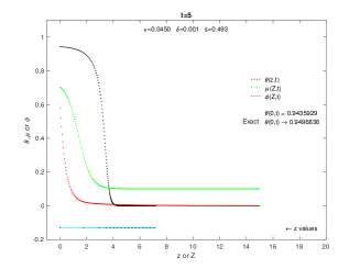
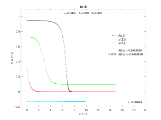
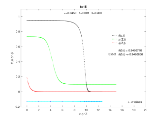
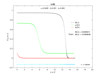
Figure 1: Simulation of the linear model based on (3.2) with constant surface flux $R(t)=0.6$ and the initial value $\theta(z,0)=0$. Parameters are given by $C=1.1$, $\epsilon=0.045$, $\delta=0.001$ and $s=\frac{\delta}{\epsilon^{2}}=0.493$.

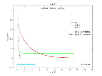
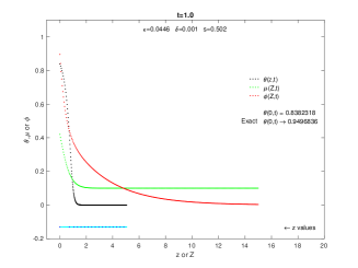
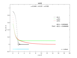
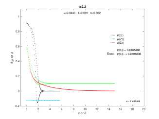
Figure 2: Simulation of the linear model with the same conditions as Figure 1, but with lattice intervals $\epsilon=0.0446$, $\delta=0.001$ and $s=\frac{\delta}{\epsilon^{2}}=0.502$. Oscillation due to numerical instability starts around $t=2.0$.

The numerical instability for (3.2) is a consequence of linear stability analysis. So one might think that we could avoid the instability by adopting the nonlinearized scheme, namely the discrete analogue of the Burgers equation. To this end, it is convenient to write down the scheme in terms of $u_{n}^{m}$ (3.15). We then have the discrete Burgers equation [34, 10, 19]

$$\begin{split}&\frac{u^{m+1}_{n}}{u^{m}_{n}}=\frac{1+\frac{\delta}{\epsilon^{2}}\left[u_{n+1}^{m}-2+\frac{1}{u_{n}^{m}}+\kappa^{m}\,\left(u_{n+1}^{m}-\frac{1}{u_{n}^{m}}\right)\right]}{1+\frac{\delta}{\epsilon^{2}}\left[u_{n}^{m}-2+\frac{1}{u_{n-1}^{m}}+\kappa^{m}\,\left(u_{n}^{m}-\frac{1}{u_{n-1}^{m}}\right)\right]},\quad\kappa^{m}=\frac{\epsilon(R^{m}-\beta)}{2a^{\frac{1}{2}}}\\[5.69054pt] &\hskip 40.0ptn=1,\ldots,N-1,\quad m=0,1,2,\ldots,\end{split}$$ (3.21)

with initial condition

$$u_{n}^{0}=\frac{1-\frac{2a^{\frac{1}{2}}}{b\epsilon}\mu^{(0)}_{n}}{1+\frac{2a^{\frac{1}{2}}}{b\epsilon}\mu^{(0)}_{n}},\quad n=0,2\ldots,N-1,$$ (3.22)

and the boundary conditions

$$u_{0}^{m}=\frac{1-\kappa^{m}}{2-a\epsilon^{2}-(1+\kappa^{m})u_{1}^{m}},\quad u_{N}^{m}=P_{N-1}.$$ (3.23)

Note that $\mu_{n}^{m}$ and $\theta_{n}^{m}$ are recovered by

$$\mu_{n}^{m}=-\frac{2a^{\frac{1}{2}}}{b\epsilon}\,\frac{u_{n}^{m}-1}{u_{n}^{m}+1},\quad\theta_{n}^{m}=b\left(1+\frac{a^{\frac{1}{2}}\epsilon}{2}\,\frac{u_{n}^{m}+1}{u_{n}^{m}-1}\right).$$ (3.24)

Then we plot $(z_{n}^{m},\theta_{n}^{m})$ with (3.18). Figure 3 illustrates the numerical result under the same condition and parameters as Figure 2. This gives the same result, and unfortunately the numerical instability is also inherited from the linear model. Indeed, choosing the lattice intervals such that $s<\frac{1}{2}$, the numerical computation is stable with sufficient precision for $\theta(0,t)$ at large $t$.

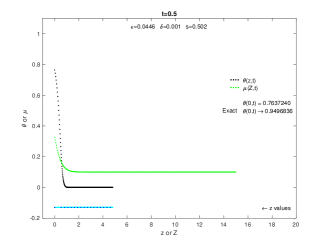
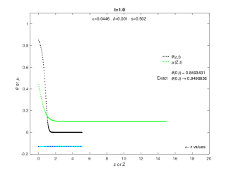
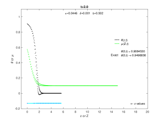
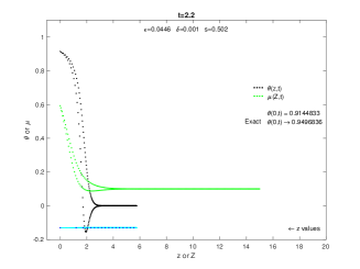
Figure 3: Simulation of the discrete Burgers model under the same conditions as Figure 2. The numerical instability is inherited from the linear model.

3.2 A stable discrete integrable model: Crank–Nicolson scheme

In order to overcome the numerical instability, a simple alternative to (3.2) with second-order accuracy is the Crank–Nicolson (CN) Scheme:

$$2\frac{\phi^{m+1}_{n}-\phi^{m}_{n}}{\delta}=F^{m}_{n}+F^{m+1}_{n},$$

$$F^{m}_{n}=\frac{\phi^{m}_{n+1}-2\phi^{m}_{n}+\phi^{m}_{n-1}}{\epsilon^{2}}+\frac{R^{m}-\beta}{a^{\frac{1}{2}}}\,\frac{\phi^{m}_{n+1}-\phi^{m}_{n-1}}{2\epsilon}.$$ (3.25)

Choosing other procedures, such as the discrete Cole-Hopf transformation (3.3) and the hodograph transformation (3.18), to be the same as the previous case, it is possible to set the initial condition by (3.6) and the large-$Z$ boundary condition as $\phi_{N}^{m}=P_{N-1}\phi_{N-1}^{m}$.

Our previous surface boundary condition (3.7) was not accurate to second-order, and hence requires modification. Our Cole–Hopf transformation (3.3) is accurate to second-order when centered on the half-node position $n+1/2$, as discussed in Remark 3.1. Accordingly, the precise place to apply the surface boundary condition when considering $\phi$ is the half node position $n=1/2$, as this corresponds to $\mu^{m}_{0}$ and $\theta^{m}_{0}$ to second-order accuracy in $\epsilon$:

$$\frac{2}{\delta}\big{(}\phi^{m+1}_{1/2}-\phi^{m}_{1/2}\big{)}=-a\big{(}\phi^{m+1}_{1/2}+\phi^{m}_{1/2}\big{)},\quad\phi^{m}_{1/2}=\frac{1}{2}\big{(}\phi^{m}_{0}+\phi^{m}_{1}\big{)}.$$ (3.26)

Here the averaging of nodes $\phi^{m+1}_{0}$ and $\phi^{m}_{0}$ on the right-hand-side of the equation ensures that the boundary condition also is of second order accuracy in $\delta$ when centered on the half node position $m+1/2$, similar to the CN scheme itself. This surface boundary condition can be alternatively expressed as

$$\phi^{m+1}_{0}+\phi^{m+1}_{1}=\frac{2-a\delta}{2+a\delta}\big{(}\phi^{m}_{0}+\phi^{m}_{1}\big{)}.$$ (3.27)

In order to compute $\phi_{n}^{m}$ ($n=0,\ldots,N-1$) we solve the following system of linear equations:

$$A\Phi=B,$$ (3.28)

$$\Phi=\left[\phi_{0}^{m+1},\phi_{1}^{m+1},\ldots,\phi_{N-1}^{m+1}\right]^{T},$$

$$B=\left[B_{0},B_{1},\ldots,B_{n-1}\right]^{T},$$

$$A\!=\!\!\left[\!\!\begin{array}[]{cccccc}A_{0,0}&A_{0,1}&0&{\scriptstyle 0}&{\scriptstyle\cdots}&{\scriptstyle 0}\\ A_{1,0}&A_{1,1}&A_{1,2}&{\scriptstyle 0}&{\scriptstyle\cdots}&{\scriptstyle 0}\\ {\scriptstyle 0}&A_{2,1}&A_{2,2}&A_{2,3}&{\scriptstyle\cdots}&{\scriptstyle 0}\\ {\scriptstyle\vdots}&{\scriptstyle\ddots}&{\scriptstyle\ddots}&{\scriptstyle\ddots}&{\scriptstyle\ddots}&{\scriptstyle\vdots}\\ {\scriptstyle 0}&{\scriptstyle\cdots}&A_{N-3,N-4}&A_{N-3,N-3}&A_{N-3,N-2}&{\scriptstyle 0}\\ {\scriptstyle 0}&{\scriptstyle\cdots}&{\scriptstyle 0}&A_{N-2,N-3}&A_{N-2,N-2}&A_{N-2,N-1}\\ {\scriptstyle 0}&{\scriptstyle\cdots}&{\scriptstyle 0}&{\scriptstyle 0}&A_{N-1,N-2}&A_{N-1,N-1}\end{array}\!\!\right]\!\!.$$ (3.36)

Here $A_{0,0}=A_{0,1}=1$ are obtained directly from (3.27), so that $B_{0}$ is given by the right-hand-side of the equation. From (3.25) we have for $k=1,2,\ldots,N-2$:

$$A_{k,k-1}=-s(1-\kappa^{m+1}),\;\;A_{k,k}=2(1+s),\;\;A_{k,k+1}=-s(1+\kappa^{m+1}),$$

$$B_{k}=s(1-\kappa^{m})\phi^{m}_{k-1}+2(1-s)\phi^{m}_{k}+s(1+\kappa^{m})\phi^{m}_{k+1}.$$ (3.37)

Finally, incorporating the boundary condition $\phi_{N}^{m}=P_{N-1}\phi_{N-1}^{m}$ gives

$$A_{N-1,N-2}=-s(1-\kappa^{m+1}),\;\;A_{N-1,N-1}=2(1+s)-sP_{N-1}(1+\kappa^{m+1}),$$

$$B_{N-1}=s(1-\kappa^{m})\phi^{m}_{N-2}+\big{[}2(1-s)+sP_{N-1}(1+\kappa^{m})\big{]}\phi^{m}_{N-1}.$$ (3.38)

Hence we obtain $\phi_{n}^{m}$ for $n=0,1,\ldots,N$ at each $m$.

Numerical results obtained are almost identical to Figure 1 for the same boundary conditions and parameters. Figure 4 shows numerical results under the same conditions, but with lattice intervals given by $\epsilon=\delta=0.02$, $s=50$. As expected, computations are stable regardless of value of $s$.

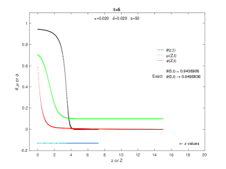
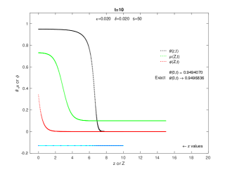
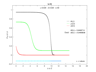
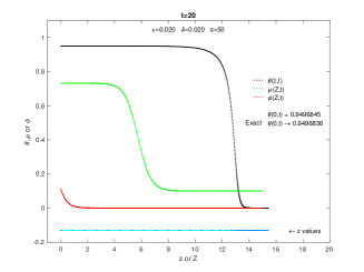
Figure 4: Simulation of the linear model based on the Crank–Nicolson scheme under the same conditions as Figure 1, but with lattice intervals $\epsilon=\delta=0.02$, $s=50$. The computation is stable and the computed value of $\theta(0,t)$ is accurate to $10^{-5}$.

Therefore, the discrete integrable model based on the Crank–Nicolson scheme may provide stable, reasonably accurate calculations for modelling groundwater infiltration.

4 Comparison with direct computation

The nonlinear equation (2.5) is amenable to direct computational solution via a variety of well established methods. If we put aside matters of theoretical interest discussed above, we have essentially established the feasibility of the Crank–Nicolson integrable model, but have not yet demonstrated any practical advantage over direct numerical approaches. While numerical methods with higher-order accuracy might be adopted to solve (2.5), they would not constitute a fair test in the present context: it should be clear that the integrable model has the potential to be generalised such that higher-order accuracy is achieved, but that is beyond the natural scope of this article. As such, in order to assess the numerical performance of our integrable model we will proceed to implement the Crank-Nicolson scheme directly on the original equation (2.5) for $\theta$:

$$2\frac{\theta^{m+1}_{n}-\theta^{m}_{n}}{\delta}=F^{m}_{n}+F^{m+1}_{n},$$

$$F^{m}_{n}=\left[\frac{a}{b}-\frac{ab}{(b-\theta^{m}_{n})^{2}}\right]\frac{\theta^{m}_{n+1}-\theta^{m}_{n-1}}{2\epsilon}$$

$$\qquad+\frac{a}{\epsilon^{2}}\frac{\theta^{m}_{n+1}-\theta^{m}_{n}}{(b-\theta^{m}_{n+1})(b-\theta^{m}_{n})}-\frac{\theta^{m}_{n}-\theta^{m}_{n-1}}{(b-\theta^{m}_{n})(b-\theta^{m}_{n-1})}.$$ (4.1)

Note that in this context the lattice parameters now relate to $z$ and $t$, so that $\theta(z,t)=\theta(n\epsilon,m\delta)=\theta^{m}_{n}$. Our initial condition is $\theta^{0}_{n}=0$ for $n=1,\ldots,N$, and under reasonable assumptions already discussed, we can assume that $\theta^{m}_{N}=0$. Our flux boundary condition at $z=0$ was given in (2.6):

$$(b-\theta)(R(t)-\beta)=ab+\frac{a}{b}(b-\theta)^{2}-\frac{a}{(b-\theta)}\frac{\partial\theta}{\partial z}.$$ (4.2)

We have discretized spatial derivatives in our integrable model both to define the Cole–Hopf transformation (3.3), and derive the initial condition (3.5). This suggests the following 2-node discretization of the above flux boundary condition

$$[(b-\theta^{m}_{0})+(b-\theta^{m}_{1})](R^{m}-\beta)=$$

$$2ab+\frac{a}{b}\big{[}(b-\theta^{m}_{0})^{2}+(b-\theta^{m}_{1})^{2}\big{]}-\frac{4a}{\epsilon}\frac{\theta^{m}_{1}-\theta^{m}_{0}}{(b-\theta^{m}_{0})+(b-\theta^{m}_{1})},$$ (4.3)

however this is only second-order accurate at $n=1/2$. The 3-node boundary condition

$$(b-\theta^{m}_{0})(R^{m}-\beta)=ab+\frac{a}{b}(b-\theta^{m}_{0})^{2}-\frac{a}{2\epsilon}\frac{-\theta^{m}_{2}+4\theta^{m}_{1}-3\theta^{m}_{0}}{(b-\theta^{m}_{0})},$$ (4.4)

is second-order accurate at $n=0$ and generally appears to perform better than (4.3). We will exclusively use (4.4) for our flux boundary condition in the computations to follow. The initial value of $\theta^{0}_{0}$ that matches $R(0)=R^{0}$ is determined from (4.4) with $\theta^{0}_{1}=\theta^{0}_{2}=0$.

Starting with known values $\theta^{m}_{n}$ for $n=0,1,\ldots,N$; equations (4.1) for $n=1,2,\ldots,N-1$, equation (4.4), and $\theta^{m+1}_{N}=0$, constitute a coupled nonlinear system of equations for the determination of $\theta^{m+1}_{n}$ ($n=0,1,\ldots,N$). A natural approach to the solution of these equations is to linearize and iterate. As such we can write equations (4.1) and (4.4) in the form

$$2\frac{\theta^{m+1}_{n,j+1}-\theta^{m}_{n}}{\delta}=\left[\frac{a}{b}-\frac{ab}{(b-\theta^{m}_{n})^{2}}\right]\frac{\theta^{m}_{n+1}-\theta^{m}_{n-1}}{2\epsilon}$$

$$\qquad+\frac{a}{\epsilon^{2}}\frac{\theta^{m}_{n+1}-\theta^{m}_{n}}{(b-\theta^{m}_{n+1})(b-\theta^{m}_{n})}-\frac{\theta^{m}_{n}-\theta^{m}_{n-1}}{(b-\theta^{m}_{n})(b-\theta^{m}_{n-1})}$$

$$\qquad+\left[\frac{a}{b}-\frac{ab}{(b-\theta^{m+1}_{n,j})^{2}}\right]\frac{\theta^{m+1}_{n+1,j+1}-\theta^{m+1}_{n-1,j+1}}{2\epsilon}$$

$$\qquad+\frac{a}{\epsilon^{2}}\frac{\theta^{m+1}_{n+1,j+1}-\theta^{m+1}_{n,j+1}}{(b-\theta^{m+1}_{n+1,j})(b-\theta^{m+1}_{n,j})}-\frac{\theta^{m+1}_{n,j+1}-\theta^{m+1}_{n-1,j+1}}{(b-\theta^{m+1}_{n,j})(b-\theta^{m+1}_{n-1,j})},$$ (4.5)

$$(b-\theta^{m+1}_{0,j+1})(R^{m+1}-\beta)=ab+\frac{a}{b}(b-\theta^{m+1}_{0,j+1})(b-\theta^{m+1}_{0,j})$$

$$\qquad-\frac{a}{2\epsilon}\frac{-\theta^{m+1}_{2,j+1}+4\theta^{m+1}_{1,j+1}-3\theta^{m+1}_{0,j+1}}{(b-\theta^{m+1}_{0,j})}.$$ (4.6)

Here instances of $\theta^{m+1}_{n}$ have been replaced by the approximations $\theta^{m+1}_{n,j}$ where $j=0,1,2,\ldots$. The initial value of these approximations can be taken to be equal to the corresponding values at the previous time step: $\theta^{m+1}_{n,0}=\theta^{m}_{n}$. Now given known $\theta^{m}_{n}$ and $\theta^{m+1}_{n,j}$ values, quantities $\theta^{m+1}_{n,j+1}$ can be calculated by solving a linear system almost identical in structure to (3.28). In practice we observe that the $\theta^{m+1}_{n,j}$ values converge quite quickly, and we have adopted a termination criteria

$$\max_{n}\left|\theta^{m+1}_{n,j+1}-\theta^{m+1}_{n,j}\right|<10^{-10},$$ (4.7)

after which the final $\theta^{m+1}_{n,j+1}$ values are accepted and the calculation proceeds to the next timestep.

It is now clear that the above process of iteration implies a greater computational burden than using the CN scheme for our integrable model. As the integrable model involves solution of a linear differential equation, only one linear system of equations (3.28) needs to be solved to obtain exact $\phi^{m+1}_{n}$ values from known $\phi^{m}_{n}$ values. Conversely, when using iteration to implement the CN scheme on equation (2.5), several linear systems of comparable difficulty to (3.28) may need to be solved to obtain sufficiently accurate values of $\theta^{m+1}_{n,j}$ beginning from known $\theta^{m}_{n}$.

As such, we can also consider direct use of the CN scheme on the equation for $\theta$ without iteration of the linearized equations (4.5), (4.6) at each timestep. That is, we simply accept the $\theta^{m+1}_{n,1}$ values as the final values of $\theta^{m+1}_{n}$. By eliminating iteration, the CN scheme applied directly to the equation (2.5) produces a solution at time $M\delta$ after the solution of only $M$ linear systems of equations — just as the integrable CN model does.

In addition to considering the limiting value of $\theta^{m}_{0}$, we can also evaluate the accuracy of our numerical methods by comparing conservation of mass. With initial condition $\theta(z,0)=0$, the relative moisture content discrepancy:

$$\frac{\displaystyle\frac{1}{2}\sum_{n=0}^{N-1}(\theta^{m}_{n}+\theta^{m}_{n+1})(z^{m}_{n+1}-z^{m}_{n})-\int_{0}^{m\delta}R(t)dt}{\displaystyle\int_{0}^{M\delta}R(t)dt}$$ (4.8)

should be of small magnitude at all times for accurate numerical schemes. Figure 5 shows the relative moisture content discrepancy for $R=0.6$. In all cases $t_{\rm max}=\tau_{\rm max}=20=M\delta$; $Z_{\rm max}=15=N\epsilon$ for the integrable CN model and $z_{\rm max}=15=N\epsilon$ for the direct CN methods. In panels (B) and (C) the noniterative direct CN scheme approaches a final relative moisture content discrepancy $\simeq-10^{-2}$. In panel (D) the noniterative direct CN methods fails altogether.

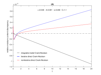
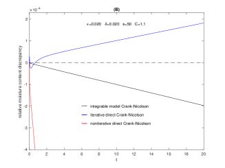
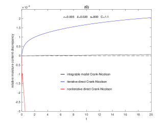
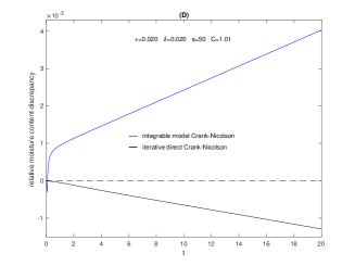
Figure 5: Comparison of conservation of mass: The CN scheme applied directly to equation (2.5) for $\theta$ with or without iteration, compared to the integrable CN model. In all cases $R(t)=0.6$ and $\theta(z,0)=0$.

In panel (A) of Figure 5 the iterative direct CN scheme involved the solution of about 80000 linear systems similar to (3.28), compared to 20000 for the noniterative direct and integrable CN schemes. In panels (B) and (C) the iterative direct CN scheme involved solution of approximately 8000 linear systems compared to 1000 for the noniterative direct and integrable CN schemes. Table 1 shows the computed values of $\theta(0,20)$ for the simulations of panels (A)–(C) of Figure 5.

Table 1: $\theta(0,20)$ values for the simulations of panels (A)–(C) of Figure 5.
As $t\to\infty$, it is known that $\theta(0,t)\to 0.9496836.$

Crank–Nicolson	$\epsilon=0.045$	$\epsilon=0.020$	$\epsilon=0.005$
implementation	$\delta=0.001$	$\delta=0.020$	$\delta=0.020$
integrable	0.9496914	0.9496845	0.9495624
iterative direct	0.9496829	0.9496828	0.9496254
noniterative direct	0.9496828	0.9496824	0.9488505

Equation (2.5) aproaches a singular nonlinear limit as $C\to 1$, and the value $C=1.01$ in panel (D) of Figure 5 could physically represent a coarse, sandy soil. As our governing equation becomes more nonlinear, the benefits of the integrable method increase. The iterative direct CN method in panel (D) involved solution of approximately 21000 linear systems, compared to only 1000 for the integrable CN method. With $C=1.01$ and $R(t)=0.6$; $\theta(0,t)\to 0.9935477$ as $t\to\infty$. Computation using the iterative direct CN method resulted in $\theta(0,20)=0.9935478$, while the integrable CN method produced $\theta(0,20)=0.9935476$.

Figure 5 shows that direct applications of the CN scheme tend to exhibit sudden changes in the moisture content discrepancy for early times, while the integrable CN model does not. This is consistent with the self-adaptive moving mesh of the integrable model providing greater accuracy for small values of $\theta$, at early times when the moisture content is increasing most rapidly.

Overall, the integrable model clearly outperforms the noniterative direct CN method, and its performance is broadly comparable to the iterative direct CN method. As detailed above, the iterative direct CN method involves a significantly greater computational effort, that yields no clear benefit when compared to the results of the integrable CN model.

5 Conclusion

In this paper we considered an integrable model of one-dimensional groundwater infiltration, a special case of the Richards equation. It takes the form of a nonlinear convection-diffusion equation with time-dependent flux boundary conditions. For the special soil model considered, the Richards equation can be transformed to the Burgers equation and the linear heat equation with an additional convective term incorporating the known surface flux.

We have constructed integrable discrete models preserving the linearizability structure above, the crucial components of this are discretization of the linear equation, as well as discretization of the Cole-Hopf and Storm transformations. Three models have been presented. The first is based on the naive Euler scheme often used in the theory of discrete integrable systems [34, 10, 19], which suffers from built-in numerical instability based on the value of $s=\delta/\epsilon^{2}$. This is not suitable for accurate computations of volumetric soil-water content. The second model is based on the discrete Burgers equation which is a nonlinearization of the Euler scheme of the first model. This inherits the numerical instability despite nonlinearization and again cannot be used for accurate calculations. Finally we propose a model based on a stable, second-order Crank–Nicolson discretization of our linear convection-diffusion equation.

We have assessed the performance of this integrable Crank–Nicolson model by comparing against the Crank–Nicolson method directly applied to the original nonlinear convection–diffusion equation. The accuracy of the final solution computed using a variety of lattice parameters was observed to be approximately equal. However, directly applying the Crank–Nicolson method to the nonlinear equation was found to involve significantly more computational effort than the integrable model as measured by the number of linear systems solved during numerical integration.

To further improve computational performance, higher-order numerical integration schemes such as higher-order Runge–Kutta methods could be applied to the transformed linear convection diffusion equation, while suffering some inconvenience in the form of more elaborate boundary condition implementation. As demonstrated for the Crank–Nicolson scheme, we expect that such higher-order integrable models will exhibit similar reductions in computational cost compared to applying the relevant higher-order schemes directly on the original nonlinear equation. As observed in this study, the reward for exploiting the integrable nature of the original equation should increase as the parameter $C$ decreases, and the nonlinearity of the original equation becomes more severe.

References

- [1] R. E. Smith, K. R. J. Smettem, P. Broadbridge and D. A. Woolhiser Infiltration theory for hydrologic applications. (American Geophysical Union, 2002).
- [2] A. W. Warrick, Soil Water Dynamics (Oxford University Press, 2003).
- [3] M.J. Ablowitz and J.F. Ladik, A nonlinear difference scheme and inverse scattering, Stud. in Appl. Math. 55(1976) 213–229.
- [4] M.J. Ablowitz and J.F. Ladik, On the solution of a class of nonlinear partial difference equations, Stud. in Appl. Math. 57(1977) 1–12.
- [5] M. J. Ablowitz B. Prinari and A.D. Trubatch, Discrete and continuous nonlinear Schrödinger systems (Cambridge University Press, 2004).
- [6] R. Hirota, Nonlinear partial difference equations. I. A difference analogue of the Korteweg-de Vries equation, J. Phys. Soc. Jpn. 43(1977) 4116–4124.
- [7] R. Hirota, Nonlinear partial difference equations. II. Discrete-time Toda equation, J. Phys. Soc. Jpn. 43(1977) 2074–2078.
- [8] R. Hirota, Nonlinear partial difference equations. III. Discrete sine-Gordon equation, J. Phys. Soc. Jpn. 43(1977) 2079–2086.
- [9] R. Hirota, Nonlinear partial difference equations. IV. Bäcklund transformation for the discrete-time Toda equation, J. Phys. Soc. Jpn. 45(1978) 321–332.
- [10] R. Hirota, Nonlinear partial difference equations. V. Nonlinear equations reducible to linear equations, J. Phys. Soc. Jpn. 46(1979) 312–319.
- [11] E. Date, M. Jimbo and T. Miwa, Method for generating discrete soliton equations.I, J. Phys. Soc. Jpn. 51(1982) 4116–4124.
- [12] E. Date, M. Jimbo and T. Miwa, Method for generating discrete soliton equations.II, J. Phys. Soc. Jpn. 51(1982) 4125–4131.
- [13] E. Date, M. Jimbo and T. Miwa, Method for generating discrete soliton equations.III, J. Phys. Soc. Jpn. 53(1983) 388–393.
- [14] E. Date, M. Jimbo and T. Miwa, Method for generating discrete soliton equations.IV, J. Phys. Soc. Jpn. 53(1983) 761–765.
- [15] E. Date, M. Jimbo and T. Miwa, Method for generating discrete soliton equations.V, J. Phys. Soc. Jpn. 53(1983) 766–771.
- [16] M. Jimbo and T. Miwa, Solitons and infinite dimensional Lie algebras, Publ. RIMS 19(1983) 943-1001.
- [17] T. Miwa, On Hirota’s difference equations, Proc. Japan Acad. Ser. A Math. Sci. 58(1982) 9–12.
- [18] A.I. Bobenko and Y.B. Suris, Discrete differential geometry (American Mathematical Society, 2008).
- [19] K. Nishinari and D. Takahashi, Analytical properties of ultradiscrete Burgers equation and rule-184 cellular automaton, J. Phys. A. Math. Theoret. 31 (1998) 5439–5450.
- [20] Discrete systems and integrability, eds. by J. Hietarinta, N. Joshi and F.W. Nijhoff, Cambridge Texts in Applied Mathematics 54 (Cambridge University Press 2016).
- [21] K. Kajiwara, M. Noumi and Y. Yamada, Geometric aspects of Painlevé equations, J. Phys. A: Math. Theor. 50(2017) 073001.
- [22] Y. Suris, The problem of integrable discretization: Hamiltonian approach, Progress in Mathematics 219 (Springer, 2003).
- [23] M. J. Ablowitz and B. M. Herbst, On homoclinic structure and numerically induced chaos for the nonlinear Schrödinger equation. SIAM J. Appl. Math. 50(1990) 339–351.
- [24] M. J. Ablowitz, B. M. Herbst and C. Schober, On the numerical solution of the sine–Gordon equation: I. Integrable discretizations and homoclinic manifolds, J. Comput. Phys. 126(1996) 299–314.
- [25] M. J. Ablowitz, C. Schober and B. M. Herbst, Numerical chaos, roundoff errors, and homoclinic manifolds, Phys. Rev. Lett. 71(1993) 2683–2686.
- [26] M. J. Ablowitz and T. R. Taha, Analitical and numerical aspects of certain nonlinear evolution equations. I. Analytical, J. Comput. Phys. 55(1984) 192–230.
- [27] B. M. Herbst and M. J. Ablowitz, Numerically induced chaos in the nonlinear Schrödinger equation. Phys. Rev. Lett. 62(1989) 2065–2068.
- [28] T. R. Taha and M. J. Ablowitz, Analytical and numerical aspects of certain nonlinear evolution equations. II. Numerical, nonlinear Schrödinger equation, J. Comput. Phys. 55(1984) 203–230.
- [29] T. R. Taha and M. J. Ablowitz, Analytical and numerical aspects of certain nonlinear evolution equations. III. Numerical, Korteweg-de Vries equation, J. Comput. Phys. 55(1984) 231–253.
- [30] T. R. Taha and M. J. Ablowitz, Analytical and numerical aspects of certain nonlinear evolution equations IV. Numerical, modified Korteweg-de Vries equation, J. Comput. Phys. 77(1988) 540–548.
- [31] B. F. Feng, K. Maruno and Y. Ohta, A self-adaptive moving mesh method for the Camassa–Holm equation, J. Comput. Appl. Math. 235(2010) 229–243.
- [32] B. F. Feng, K. Maruno and Y. Ohta, Integrable discretizations of the short pulse equation, J. Phys. A: Math. Theor. 43(2010) 085203.
- [33] B. F. Feng, K. Maruno and Y. Ohta, Self-adaptive moving mesh schemes for short pulse type equations and their Lax pairs. Pacific Journal of Mathematics for Industry 6(2014) 1–14.
- [34] R.H. Heredero, D. Levi and P. Winternitz, Symmetries of the discrete Burgers equation. J. Phys. A: Math. Gen. 32(1999) 2685–2695.
- [35] P. Broadbridge and I. White, Constant rate rainfall infiltration: a versatile nonlinear model 1. Analytic solution. Water Resour. Res. 24(1988) 145–154.
- [36] I. White and P. Broadbridge, Constant rate rainfall infiltration: a versatile nonlinear model 2. Applications of solutions, Water Resour. Res. 24(1988) 155–162.
- [37] G. Kirchhoff, Vorlesungen über die Theorie der Wärme, Barth, 1894.
- [38] M. L. Storm, Heat conduction in simple metals, J. Appl. Phys. 22(1951) 940–951.
- [39] R. Courant and K. O. Friedrichs, Supersonic flow and shock waves, Interscience Publishers, 1948.
- [40] Disctete integrable systems, eds. by B. Grammaticos, Y. Kosmann-Schwarzbach and T. Tamizhmani, Lecture Notes in Physics 644 (Springer, 2004).
- [41] B.-F. Feng, J. Inoguchi, K. Kajiwara, K. Maruno, and Y. Ohta, Discrete integrable systems and hodograph transformations arising from motions of discrete plane curves. J. Phys. A: Math. Theor. 44(2011) 395201.
- [42] B.-F. Feng, J. Inoguchi, K. Kajiwara, K. Maruno, and Y. Ohta, Integrable discretizations of the Dym equation. Front. Math. China 8(2013) 1017–1029.