Analysis of Approximate Message Passing
with A Class of Non-Separable Denoisers

Abstract

Approximate message passing (AMP) is a class of efficient algorithms for solving high-dimensional linear regression tasks where one wishes to recover an unknown signal $\beta_{0}$ from noisy, linear measurements $y=A\beta_{0}+w$. When applying a separable denoiser at each iteration of the algorithm, the performance of AMP (for example, the mean squared error of its estimate) can be accurately tracked by a simple, scalar recursion called state evolution. Separable denoisers are sufficient when the unknown signal has independent entries, however, in many real-world applications, like image or audio signal reconstruction, the signal contains dependencies between entries. In these cases, a coordinate-wise independence structure is not a good approximation to the true prior of the unknown signal. In this paper we assume the unknown signal has dependent entries, and using a class of non-separable sliding-window denoisers, we prove that a new form of state evolution still accurately predicts AMP performance. This is an early step in understanding the role of non-separable denoisers within AMP, and will lead to a characterization of more general denoisers in problems including compressive image reconstruction.

1 Introduction

In this work, we study the high-dimensional linear regression model, where one wishes to recover an unknown signal $\beta_{0}\in\mathbb{R}^{N}$ from noisy observations as in the following model:

$$y=A\beta_{0}+w,$$ (1)

where $y\in\mathbb{R}^{n}$ is the output, $A\in\mathbb{R}^{n\times N}$ is a known measurement matrix, and $w\in\mathbb{R}^{n}$ is zero-mean noise with finite variance $\sigma^{2}$. We assume that the ratio of the dimensions of the measurement matrix is a constant value, $\delta:=n/N$, with $\delta\in(0,\infty)$.

Approximate message passing (AMP) [1, 2, 3, 4, 5] is a class of low-complexity, scalable algorithms studied to solve the high-dimensional regression task of (1). The performance of AMP depends on a sequence of functions $\{\eta_{t}\}_{t\geq 0}$ used to generate a sequence of estimates $\{\beta^{t}\}_{t\geq 0}$ from auxiliary observation vectors computed in every iteration of the algorithm. A nice property of AMP is that under some technical conditions these observation vectors can be approximated as the input signal $\beta_{0}$ plus independent and identically distributed, or i.i.d., Gaussian noise. This fact allows one to choose functions $\{\eta_{t}\}_{t\geq 0}$ based on statistical knowledge of $\beta_{0}$, for example, a common choice is for $\eta_{t}$ to be the Bayes-optimal estimator of $\beta_{0}$ conditional on the value of the observation vector. For this reason, the functions $\{\eta_{t}\}_{t\geq 0}$ are referred to as ‘denoisers.’

Previous analysis of the performance of AMP only considers denoisers $\{\eta_{t}\}_{t\geq 0}$ that act coordinate-wise when applied to a vector; such functions are referred to as separable. If the unknown signal $\beta_{0}$ has a prior distribution assuming i.i.d. entries, restricting consideration to only separable denoisers causes no loss in performance. However, in many real-world applications, the unknown signal $\beta_{0}$ contains dependencies between entries and therefore a coordinate-wise independence structure is not a good approximation for the prior of $\beta_{0}$. For example, when the signals are images [6, 7] or sound clips [8], non-separable denoisers outperform reconstruction techniques based on over-simplified i.i.d. models. In such cases, a more appropriate model might be a finite memory model, well-approximated with a Markov chain prior. In this paper, we extend the previous performance guarantees for AMP to a class of non-separable sliding-window denoisers, whose promising empirical performance was shown by Ma et al. [8], when the unknown signal is produced by a Markov chain starting from its stationary distribution.

When the measurement matrix $A$ has i.i.d. Gaussian entries and the empirical distribution of the unknown signal $\beta_{0}$ converges to some probability distribution on $\mathbb{R}$, Bayati and Montanari [3] proved that at each iteration the performance of AMP can be accurately predicted by a simple, scalar iteration referred to as state evolution in the large system limit ($n,N\to\infty$ such that $\frac{n}{N}=\delta$ is a constant). For example, if $\beta^{t}$ is the estimate produced by AMP at iteration $t$, their result implies that the normalized squared error, $\frac{1}{N}\left\lVert\beta^{t}-\beta_{0}\right\rVert^{2}$, and other performance measures converge to known values predicted by state evolution using the prior distribution of $\beta_{0}$. Recently, Rush and Venkataramanan [9] provided a concentration version of the asymptotic result when the prior distribution of $\beta_{0}$ is i.i.d. sub-Gaussian. The result implies that the probability of $\epsilon$-deviation between various performance measures and their limiting constant values fall exponentially in $n$. Extensions of AMP performance guarantees beyond separable denoisers have been considered in special cases [10, 11] for certain classes of block-separable denoisers that allow dependencies within blocks of the signal $\beta_{0}$ with independence across blocks. However these settings are more restricted than the types of dependencies we consider here.

1.1 AMP Algorithm for Sliding-Window Denoiser

The AMP algorithm, in the case of a dependent signal, generates successive estimates of the unknown vector denoted by $\beta^{t}\in\mathbb{R}^{N}$ for $t=1,2,\ldots$. These values are calculated as follows: given the observed vector $y$, set $\beta^{0}=0$, the all-zeros vector. For $t=0,1,\ldots$, fix $k\geq 0$ an integer, and AMP computes

$$z^{t} =y-A\beta^{t}+\frac{z^{t-1}}{n}\sum_{i=k+1}^{N-k}\eta_{t-1}^{\prime}([A^{*}z^{t-1}+\beta^{t-1}]_{i-k}^{i+k}),$$ (2)

$$\beta^{t+1}_{i} =\begin{cases}\eta_{t}([A^{*}z^{t}+\beta^{t}]_{i-k}^{i+k})\quad&\text{ if }k+1\leq i\leq N-k,\\ 0\quad&\text{ otherwise},\end{cases}$$ (3)

for an appropriately-chosen sequence of non-separable denoiser functions $\{\eta_{t}\}_{t\geq 0}:\mathbb{R}^{2k+1}\to\mathbb{R}$, where the notation

$$[x]_{i-k}^{i+k}=(x_{i-k},\ldots,x_{i+k})\in\mathbb{R}^{2k+1}\quad\text{ for }\quad x\in\mathbb{R}^{N},$$

and $A^{*}$ denotes the transpose of $A$. We let $\eta^{\prime}_{t}$ denote the partial derivative of $\eta_{t}$ with respect to (w.r.t.) the $(k+1)^{th}$ coordinate, or the center element, assuming the function is differentiable. Quantities with a negative index in (2) and (3) are set to zero.

1.2 Contributions and Outline

Our main result proves concentration for order-2 pseudo-Lipschitz (PL) loss functions for the AMP estimate of (3) at any iteration $t$ of the algorithm to constant values predicted by the state evolution equations. We envision that our work in understanding the role of sliding-window denoisers within AMP is an early step in characterizing the role of non-separable denoisers within AMP. This work will lead to a characterization of more general denoisers in problems including compressive image reconstruction [6, 7].

To characterize AMP performance for sliding-window denoisers when the input signal is a Markov chain, we need concentration inequalities for PL functions of Markov chains and sequences of Gaussian vectors that are constructed in a certain way. Specifically, in the constructed sequences, successive elements are successive $(2k+1)$-length overlapping blocks of some original sequences (another Markov chain or Gaussian sequence, respectively), as suggested by the structure of the denoiser $\eta_{t}$ in (3). These concentration results are proved in Lemmas D.5 and D.6 in Appendix D.

The rest of the paper is organized as follows. Section 2 provides model assumptions, state evolution for sliding-window denoisers, and the main performance guarantee (Theorem 1), a concentration result for PL loss functions acting on the AMP estimate from (3) to the state evolution predictions. Section 3 proves Theorem 1 with a proof based on two technical results, Lemma 2 and Lemma 3, which are proved in Section 4.

2 Main Results

2.1 Definitions and Assumptions

First we include definitions of properties of Markov chains that will be useful to clarify our assumptions on the unknown signal $\beta_{0}$.

Definition 2.1.

Consider a Markov chain on a state space $S$ with transition probability measure $r(x,dy)$ and stationary distribution $\gamma$. Denote the set of all $\gamma$-square-integrable functions by $L^{2}(\gamma):=\{f:\mathbb{R}\rightarrow\mathbb{R}:\int_{S}|f(x)|^{2}\gamma(dx)<\infty\}$. Define a linear operator $R$ associated with $r(x,dy)$ as $Rf(x):=\int_{S}f(y)r(x,dy)$ for $f\in L^{2}(\gamma)$. The chain is said to be geometrically ergodic on $L^{2}(\gamma)$ if there exists $0<\rho<1$ such that for each probability measure $\nu$ that satisfies $\int_{S}|\frac{d\nu}{d\gamma}|^{2}d\gamma<\infty$, there is a constant $C_{\nu}<\infty$ such that

$$\sup_{A\in\mathcal{B}(S)}\left\lvert\int_{S}r^{n}(x,A)\nu(dx)-\gamma(A)\right\rvert<C_{\nu}\rho^{n},\qquad n\in\mathbb{N},$$

where $\mathcal{B}(S)$ is the Borel sigma-algebra on $S$ and $r^{n}(x,dy)$ denotes the $n$-step transition probability measure. In other words, geometrical ergodicity means the chain converges to its stationary distribution $\gamma$ geometrically fast. The chain is said to be reversible if $r(x,dy)\gamma(dx)=r(y,dx)\gamma(dy)$. Moreover, a chain is said to have a spectral gap on $L^{2}(\gamma)$ if

$$g_{2}:=1-\sup\{\lambda\in\Lambda:\lambda\neq 1\}>0,$$

where $\Lambda$ is a set of values for $\lambda$ such that $(\lambda\mathsf{I}-R)^{-1}$ does not exist as a bounded linear operator on $L^{2}(\gamma)$. Note that for a countable state space $S$, $\Lambda$ is the set of all eigenvalues of the transition probability matrix, hence $g_{2}$ is the distance between the largest and the second largest eigenvalues.

It has been proved that a Markov chain has spectral gap on $L^{2}(\gamma)$ if and only if it is reversible and geometrically ergodic [12]. We use the existence of a spectral gap to prove concentration results for PL functions with dependent input, where the dependence is characterized by a Markov chain. Such concentration results are crucial for obtaining the main technical lemma, Lemma 3, and hence our main result, Theorem 1. If the spectral gap does not exist, meaning that $g_{2}=0$, then our proof only bounds the probability of tail events in Lemma 3 by constant 1, which is useless.

With this definition, we now clarify the assumptions under which our result is proved.

Assumptions:

Signal: Let $S\subset\mathbb{R}$ be a bounded state space (countable or uncountable). We assume that the signal $\beta_{0}\in S^{N}$ is produced by a time-homogeneous, reversible, geometrically ergodic Markov chain in its (unique) stationary distribution. Note that this means the ‘sequence’ $\beta_{0_{1}},\beta_{0_{2}},\ldots,\beta_{0_{N}}$, where $\beta_{0_{i}}$ is element $i$ of $\beta_{0}$, forms a Markov chain. We refer to the stationary distribution as $\gamma_{\beta}$.

Denoiser functions: The denoiser functions $\eta_{t}:\mathbb{R}^{2k+1}\rightarrow\mathbb{R}$ used in (3) are assumed to be Lipschitz for each $t>0$ and differentiable w.r.t. the $(k+1)^{th}$ (middle) coordinate with bounded derivative denoted by $\eta_{t}^{\prime}$. Further, the derivative $\eta_{t}^{\prime}$ is assumed to be differentiable with bounded derivative. Note that this implies $\eta_{t}^{\prime}$ is Lipschitz. (It is possible to put a weaker condition on $\eta_{t}$ as in [9]. That is, $\eta_{t}$ is Lipschitz, hence weakly differentiable with bounded derivative. The weak derivative w.r.t. the $(k+1)^{th}$ coordinate, denoted by $\eta_{t}^{\prime}$, is assumed to be differentiable except at a finite number of points; the derivative of $\eta_{t}^{\prime}$ is assumed to be bounded when it exists.)

Matrix: The entries of the matrix $A$ are i.i.d. $\sim\mathcal{N}(0,1/n)$.

Noise: The entries of the measurement noise vector $w$ are i.i.d. according to some sub-Gaussian distribution $p_{w}$ with mean 0 and finite variance $\sigma^{2}$. The sub-Gaussian assumption implies that for all $\epsilon\in(0,1)$,

$$P\left(\left\lvert\frac{1}{n}\|w\|^{2}-\sigma^{2}\right\rvert\geq\epsilon\right)\leq Ke^{-\kappa n\epsilon^{2}}$$

for some constants $K,\kappa>0$ [13].

2.2 Performance Guarantee

As mentioned in Section 1, the behavior of the AMP algorithm is predicted by a simple, scalar iteration referred to as state evolution, which we introduce here. Let the stationary distribution $\gamma_{\beta}$ and the transition probability measure $r(x,dy)$ define the prior distribution for the unknown vector $\beta_{0}$ in (1). Let the random variable $\beta\in S$ be distributed as $\gamma_{\beta}$ and the random vector $\underline{\beta}\in S^{2k+1}$ be distributed as $\pi$, where

$$\pi(dx)=\pi((dx_{1},...,dx_{2k+1}))=\prod_{i=2}^{2k+1}r(x_{i-1},dx_{i})\gamma_{\beta}(dx_{1})$$ (4)

is the probability of seeing such a length-$(2k+1)$ sequence in the $\beta_{0}$ Markov chain (i.e. it is the $(2k+1)$-dimension marginal distribution of $\beta_{0}$). Define $\sigma_{\beta}^{2}=\mathbb{E}[\beta^{2}]>0$ and $\sigma_{0}^{2}=\sigma_{\beta}^{2}/\delta$. Iteratively define the quantities $\{\sigma_{t}^{2}\}_{t\geq 1}$ and $\{\tau_{t}^{2}\}_{t\geq 0}$ as follows,

$$\begin{split}\tau_{t}^{2}&=\sigma^{2}+\sigma_{t}^{2},\\ \sigma_{t+1}^{2}&=\frac{1}{\delta}\left((1-w_{k})\mathbb{E}\left[\left(\eta_{t}(\underline{\beta}+\tau_{t}\underline{Z})-\underline{\beta}_{k+1}\right)^{2}\right]+w_{k}\sigma_{\beta}^{2}\right),\end{split}$$ (5)

with $\underline{\beta}_{k+1}$ the $(k+1)^{th}$ entry of $\underline{\beta}$, $\underline{Z}\in\mathbb{R}^{2k+1}\sim\mathcal{N}(0,\mathbb{I}_{2k+1})$ independent of $\underline{\beta}$, $w_{k}=\frac{2k}{N}$, and $\delta=\frac{n}{N}$.

Theorem 1 provides our main performance guarantee, which is a concentration inequality for pseudo-Lipschitz (PL) loss functions.

Theorem 1.

With the assumptions of Section 2.1, for any order-$2$ pseudo-Lipschitz function $\phi:\mathbb{R}^{2}\rightarrow\mathbb{R}$, $\epsilon\in(0,1)$, and $t\geq 0$,

$$P\left(\left\lvert\sum_{i=k+1}^{N-k}\frac{\phi(\beta^{t+1}_{i},\beta_{0_{i}})}{N-2k}-\mathbb{E}[\phi(\eta_{t}(\underline{\beta}+\tau_{t}\underline{Z}),\underline{\beta}_{k+1})]\right\lvert\geq\epsilon\right)\leq K_{k,t}e^{-\kappa_{k,t}n\epsilon^{2}}.$$ (6)

In the expectation in (6), $\underline{\beta}\in S^{2k+1}\sim\pi$, $\underline{\beta}_{k+1}$ is the $(k+1)^{th}$ element of $\underline{\beta}$, and $\underline{Z}\in\mathbb{R}^{2k+1}\sim\mathcal{N}(0,\mathbb{I}_{2k+1})$ independent of $\underline{\beta}$. The constant $\tau_{t}$ is defined in (5) and constants $K_{k,t},\kappa_{k,t}>0$ depend on the iteration index $t$ and half window-size $k$, but not on $n$ or $\epsilon$ and are not exactly specified.

Remarks:

(1) The probability in (6) is w.r.t. the product measure on the space of the matrix $A$, signal $\beta_{0}$, and noise $w$.

(2) Theorem 1 shows concentration for the loss when considering only the inner $N-2k$ elements of the signal. This is due to the nature of the sliding-window denoiser, which updates each element of the estimate $\beta^{t}$ using the $k$ elements on either side of that location. In practice, as in Ma et al. [8], one could run a slightly different algorithm than that given in (2)-(3): instead of setting the end elements, meaning the first $k$ and last $k$ elements, of the estimate $\beta^{t}$ equal to $0$, update these elements using the sliding-window denoiser but with missing input values replaced by the median of the other inputs. Such a strategy shows good empirical performance – even at the end elements – and suggests that the concentration result of Theorem 1 could be extended to show concentration for the loss of the full signal. Proving this requires a delicate handling of the end elements and is left for future research.

(3) The state evolution constants $\{\tau_{t}^{2}\}_{t\geq 0}$ defined in (5) are the sum of $\sigma^{2}$ and two weighted terms, where the weight depends on $k$, the length of the window in the sliding-window denoiser. Since we only estimate the middle $N-2k$ elements of the signal, as $k$ increases the state evolution constants $\{\tau_{t}^{2}\}_{t\geq 0}$ depend more on the second moment of the one-dimensional marginals of the original signal, corresponding to the estimation error in the un-estimated part of the signal.

(4) By choosing PL loss, $\phi(a,b)=(a-b)^{2}$, Theorem 1 gives the following concentration result for the mean squared error of the middle $N-2k$ coordinates of the estimates. For all $t\geq 0$,

$$P\left(\left\lvert\sum_{i=k+1}^{N-k}\frac{(\beta^{t+1}_{i}-\beta_{0_{i}})^{2}}{N-2k}-\frac{n(\tau_{t+1}^{2}-\sigma^{2})-2k\sigma_{\beta}^{2}}{N-2k}\right\lvert\geq\epsilon\right)\leq K_{k,t}e^{-\kappa_{k,t}n\epsilon^{2}},$$

with $\tau_{t+1}^{2}$ defined in (5). A numerical example demonstrating that the MSE of the AMP estimates $\{\beta^{t}\}_{t\geq 0}$ is tracked by the state evolution iteration (5) is proved in Section 2.3.

2.3 A Numerical Example

We now provide a concrete numerical example where AMP is used to estimate $\beta_{0}$ from the linear system (1), when the entries of $\beta_{0}$ form a Markov chain on state space $\{0,1\}$ starting from its stationary distribution. The transition probability measure is $r(0,1)=3/70$ and $r(1,0)=1/10$, which yields a unique stationary distribution $\gamma_{\beta}(1)=1-\gamma_{\beta}(0)=3/10$.

We define the denoiser function $\eta_{t}$ in (3) as the Bayesian sliding-window denoiser. Note that an important key property of AMP is the following: for large $n$ and for $k+1\leq i\leq N-k$, the observation vector $[A^{*}z^{t}+\beta^{t}]_{i-k}^{i+k}$ used as input to the estimation function in (3) is approximately distributed as $\underline{\beta}+\tau_{t}\underline{Z}$, where $\underline{\beta}\sim\pi$ with $\pi(x_{1},...,x_{2k+1}):=\prod_{i=2}^{2k+1}r(x_{i-1},x_{i})\gamma_{\beta}(x_{1}),$ $\underline{Z}\sim\mathcal{N}(0,\textsf{I}_{2k+1})$ independent of $\underline{\beta}$, and $\tau_{t}$ is defined in (5).

The above property gives us a natural way to define the Bayesian sliding-window denoiser. That is, suppose $\underline{V}_{i}=[A^{*}z^{t}+\beta^{t}]_{i-k}^{i+k}\in\mathbb{R}^{2k+1}$. Then, define

$$\eta_{t}([A^{*}z^{t}+\beta^{t}]_{i-k}^{i+k})=\eta_{t}(\underline{V}_{i}):=\mathbb{E}\left[\underline{\beta}_{k+1}\left|\underline{\beta}+\tau_{t}\underline{Z}=\underline{V}_{i}\right.\right],$$

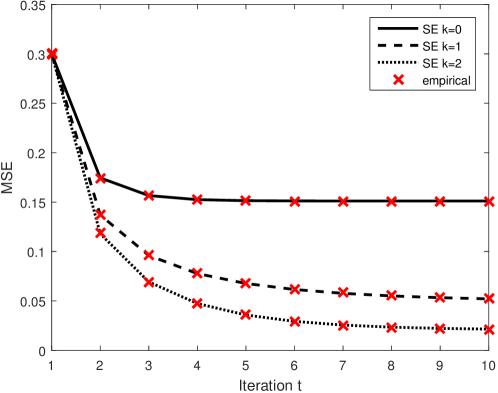
where $\underline{\beta}_{k+1}$ denotes the $(k+1)^{th}$ element of $\underline{\beta}$. Figure 1 shows that the mean squared error (MSE) achieved by AMP with the non-separable sliding-window denoiser defined above is tracked by state evolution at every iteration.

Notice that when $k=0$, the denoisers $\{\eta_{t}\}_{t\geq 0}$ are separable and the empirical distribution of $\beta_{0}$ converges to the stationary probability distribution $\gamma_{\beta}$ on $\mathbb{R}$. For this case, the state evolution analysis for AMP with separable denoisers ($k=0$) was justified by Bayati and Montanari [3]. However, it can be seen in Figure 1 that the MSE achieved by the separable denoiser ($k=0$) is significantly higher (worse) than that achieved by the non-separable denoisers ($k=1,2$).

Figure 1: The plot provides the results of a numerical example to demonstrate the validation of state evolution of AMP with non-separable sliding-window denoisers. The black curves are theoretical state evolution predictions given by (5) with three different half window-sizes, $k$. The red crosses are empirical MSE achieved by the AMP algorithm defined in (2) and (3). ($N=10,000$, $\delta=0.3$, $\sigma^{2}=0.1$.)

3 Proof of Theorem 1

The proof of Theorem 1 follows the work of Rush and Venkataramanan [9], with modifications for the dependent structure of the unknown vector $\beta_{0}$ in (1). For this reason, we use much of the same notation. The main ingredients in the proof of Theorem 1 are two technical lemmas corresponding to [9, Lemmas 4 and 5]. We first cover some preliminary results and establish notation used in the proof. We then discuss the lemmas used to prove Theorem 1.

3.1 Proof Notation

As mentioned above, in order to streamline the proof of our technical lemmas we use notation similar to [9] and consequently to [3]. As in the previous work, the technical lemmas are proved for a more general recursion which we define in the following, with AMP being a specific example of the general recursion as shown below.

Given noise $w\in\mathbb{R}^{n}$ and unknown signal $\beta_{0}\in S^{N}$, fix the half-window-size $k>0$ an integer, define column vectors $h^{t+1},q^{t+1}\in\mathbb{R}^{N}$ and $b^{t},m^{t}\in\mathbb{R}^{n}$ for $t\geq 0$ recursively as follows, starting with initial condition $q^{0}\in\mathbb{R}^{N}$:

$$\begin{split}h^{t+1}:=A^{*}m^{t}-\xi_{t}q^{t},\qquad&q^{t}_{i}:=\begin{cases}f_{t}([h^{t}]_{i-k}^{i+k},[\beta_{0}]_{i-k}^{i+k}),\qquad&\text{ if }k+1\leq i\leq N-k,\\ -\beta_{0_{i}},\qquad&\text{ otherwise},\end{cases}\\ b^{t}:=Aq^{t}-\lambda_{t}m^{t-1},\qquad&m^{t}:=g_{t}(b^{t},w),\end{split}$$ (7)

with scalar values $\xi_{t}$ and $\lambda_{t}$ defined as

$$\xi_{t}:=\frac{1}{n}\sum_{i=1}^{n}g_{t}^{\prime}(b^{t}_{i},w_{i}),\quad\lambda_{t}:=\frac{1-w_{k}}{\delta(N-2k)}\sum_{i=k+1}^{N-k}f_{t}^{\prime}([h^{t}]_{i-k}^{i+k},[\beta_{0}]_{i-k}^{i+k}),$$ (8)

where $w_{k}=2k/N$. For the derivatives in (8), the derivative of $g_{t}:\mathbb{R}^{2}\rightarrow\mathbb{R}$ is with respect to the first argument and the derivative of $f_{t}:\mathbb{R}^{2(2k+1)}\rightarrow\mathbb{R}$ is with respect to the $(k+1)^{th}$, or center coordinate, of the first argument. The functions $\{f_{t}\}_{t\geq 0}$, and $\{g_{t}\}_{t\geq 0}$ are assumed to be Lipschitz continuous and differentiable with bounded derivatives $g_{t}^{\prime}$ and $f_{t}^{\prime}$. Further, $g^{\prime}_{t}$ and $f^{\prime}_{t}$ are each assumed to be differentiable in the first argument with bounded derivative. For $f^{\prime}_{t}$ this means that we assume the first $2k+1$ partial derivatives exist and are bounded.

Recall that the unknown vector $\beta_{0}\in S^{N}$ is assumed to have a Markov chain prior with transition probability measure $r(x,dy)$ and stationary probability measure $\gamma_{\beta}$. Let $\beta\in S\sim\gamma_{\beta}$ and $\underline{\beta}\in S^{2k+1}\sim\pi$ where $\pi$ is defined in (4). Note that $\pi$ is the $(2k+1)$-dimension marginal distribution of $\beta_{0}$ and $\gamma_{\beta}$ is the one-dimensional marginal distribution.

Let $\underline{0}\in\mathbb{R}^{2k+1}$ be a vector of zeros. Define

$$\sigma_{\beta}^{2}:=\mathbb{E}[\beta^{2}],\quad\text{ and }\quad\sigma_{0}^{2} :=\frac{1}{\delta}\left((1-w_{k})\mathbb{E}\left[f_{0}^{2}(\underline{0},\underline{\beta})\right]+w_{k}\sigma_{\beta}^{2}\right)>0.$$ (9)

Further, let

$$q^{0}_{i}:=\begin{cases}f_{0}(\underline{0},[\beta_{0}]_{i-k}^{i+k}),\qquad&\text{ if }k+1\leq i\leq N-k\\ -\beta_{0_{i}},\qquad&\text{ otherwise}\end{cases}$$ (10)

and assume that there exist constants $K,\kappa>0$ such that

$$P\left(\left\lvert\frac{1}{n}\left\lVert q^{0}\right\rVert^{2}-\sigma_{0}^{2}\right\lvert\geq\epsilon\right)\leq Ke^{-\kappa n\epsilon^{2}}.$$ (11)

Define the state evolution scalars $\{\tau_{t}^{2}\}_{t\geq 0}$ and $\{\sigma_{t}^{2}\}_{t\geq 1}$ for the general recursion as follows.

$$\tau_{t}^{2}:=\mathbb{E}\left[(g_{t}(\sigma_{t}Z,W))^{2}\right],\quad\quad\sigma_{t}^{2}:=\frac{1}{\delta}\left((1-w_{k})\mathbb{E}\left[(f_{t}(\tau_{t-1}\underline{Z},\underline{\beta}))^{2}\right]+w_{k}\sigma_{\beta}^{2}\right),$$ (12)

where random variables $W\sim p_{w}$ and $Z\sim\mathcal{N}(0,1)$ and random vectors $\underline{\beta}\in S^{2k+1}\sim\pi$ and $\underline{Z}\in\mathbb{R}^{2k+1}\sim\mathcal{N}(0,\mathsf{I}_{2k+1})$ are independent. We assume that both $\sigma_{0}^{2}$ and $\tau_{0}^{2}$ are strictly positive.

We note that the AMP algorithm introduced in (2) and (3) is a special case of the general recursion introduced (7) and (8). Indeed, define the following vectors recursively for $t\geq 0$, starting with $\beta^{0}=0$ and $z^{0}=y$.

$$\begin{split}h^{t+1}=\beta_{0}-(A^{*}z^{t}+\beta^{t}),\qquad&q^{t}=\beta^{t}-\beta_{0},\\ b^{t}=w-z^{t},\qquad&m^{t}=-z^{t}.\end{split}$$ (13)

It can be verified that these vectors satisfy (7) and (8) with Lipschitz functions

$$f_{t}(\underline{a},[\beta_{0}]_{i-k}^{i+k})=\eta_{t-1}\left([\beta_{0}]_{i-k}^{i+k}-\underline{a}\right)-\beta_{0_{i}},\quad\text{ and }\quad g_{t}(b,w)=b-w,$$ (14)

where $\underline{a}\in\mathbb{R}^{2k+1}$ and $b\in\mathbb{R}$. Using $f_{t},g_{t}$ defined in (14) in (12) yields the expressions for $\sigma_{t}^{2},\tau_{t}^{2}$ in (5). We note that by Lemma D.6 with $d=1$ and $f(x):=x^{2}$,

$$P\left(\left\lvert\frac{1}{N}\|\beta_{0}\|^{2}-\sigma_{\beta}^{2}\right\rvert\geq\epsilon\right)\leq Ke^{-\kappa N\epsilon^{2}},$$ (15)

and so for the AMP algorithm using $f_{t}$ from (14) in (10), assumption (11) is satisfied.

In what follows, the notation matches that of [9] but is repeated here for completeness. In the remaining analysis, the general recursion given in (7) and (8) is used. We can write vector equations to represent the recursion as follows: for all $t\geq 0$,

$$b^{t}+\lambda_{t}m^{t-1}=Aq^{t},\quad\text{ and }\quad h^{t+1}+\xi_{t}q^{t}=A^{*}m^{t}.$$ (16)

This yields matrix equations $X_{t}=A^{*}M_{t}$ and $Y_{t}=AQ_{t},$ where we define the individual matrices as

$$\begin{split}X_{t}:=[h^{1}+\xi_{0}q^{0}\mid h^{2}+\xi_{1}q^{1}\mid\ldots\mid h^{t}+\xi_{t-1}q^{t-1}],&\qquad Q_{t}:=[q^{0}\mid\ldots\mid q^{t-1}],\\ Y_{t}:=[b^{0}\mid b^{1}+\lambda_{1}m^{0}\mid\ldots\mid b^{t-1}+\lambda_{t-1}m^{t-2}],&\qquad M_{t}:=[m^{0}\mid\ldots\mid m^{t-1}]\\ \Xi_{t}:=\text{diag}(\xi_{0},\ldots,\xi_{t-1})&\qquad H_{t}:=[h^{1}|\ldots|h^{t}],\\ \Lambda_{t}:=\text{diag}(\lambda_{0},\ldots,\lambda_{t-1})&\qquad B_{t}:=[b^{0}|\ldots|b^{t-1}].\end{split}$$ (17)

In the above, $[c_{1}\mid c_{2}\mid\ldots\mid c_{k}]$ denotes a matrix with columns $c_{1},\ldots,c_{k}$ and $M_{0}$, $Q_{0}$, $B_{0}$, $H_{0}$, and $\Lambda_{0}$ are defined to be the all-zero vector. From the above matrix definitions we have the following matrix equations $Y_{t}=B_{t}+\Lambda_{t}[0|M_{t-1}]$ and $X_{t}=H_{t}+\Xi_{t}Q_{t}.$

The values $m^{t}_{\|}$ and $q^{t}_{\|}$ are projections of $m^{t}$ and $q^{t}$ onto the column space of $M_{t}$ and $Q_{t}$, with $m^{t}_{\perp}:=m^{t}-m^{t}_{\|},$ and $q^{t}_{\perp}:=q^{t}-q^{t}_{\|}$ being the projections onto the orthogonal complements of $M_{t}$ and $Q_{t}$. Finally, define the vectors

$$\alpha^{t}:=(\alpha^{t}_{0},\ldots,\alpha^{t}_{t-1})^{*},\qquad\gamma^{t}:=(\gamma^{t}_{0},\ldots,\gamma^{t}_{t-1})^{*}$$ (18)

to be the coefficient vectors of the parallel projections, i.e.,

$$m^{t}_{\|}:=\sum_{i=0}^{t-1}\alpha^{t}_{i}m^{i},\qquad q^{t}_{\|}:=\sum_{i=0}^{t-1}\gamma^{t}_{i}q^{i}.$$ (19)

The technical lemma, Lemma 3, shows that for large $n$, the entries of the vectors $\alpha^{t}$ and ${\gamma}^{t}$ concentrate to constant values which are defined in the following section.

3.2 Concentrating Constants

Recall that $\beta_{0}\in S^{N}$ is the unknown vector to be recovered and $w\in\mathbb{R}^{n}$ is the measurement noise. Using the definitions in (13), note that the vector $h^{t+1}$ is the noise in the observation $A^{*}z^{t}+\beta^{t}$ (from the true $\beta_{0}$), while $q^{t}$ is the error in the estimate $\beta^{t}$. The technical lemma will show that $h^{t+1}$ can be approximated as i.i.d. $\mathcal{N}(0,\tau_{t}^{2})$ in functions of interest for the problem, namely when used as input to PL functions, and $b^{t}$ can be approximated as i.i.d. $\mathcal{N}(0,\sigma_{t}^{2})$ in PL functions. Moreover, the deviations of the quantities $\frac{1}{n}\|m^{t}\|^{2}$ and $\frac{1}{n}\|q^{t}\|^{2}$ from $\tau_{t}^{2}$ and $\sigma_{t}^{2}$, respectively, fall exponentially in $n$. In this section we introduce the concentrating values for various inner products of the values $\{h^{t},m^{t},q^{t},b^{t}\}$ that are used in Lemma 3.

First define the concentrating values for $\lambda_{t+1}$ and $\xi_{t}$ defined in (8) as

$$\hat{\lambda}_{t+1}:=\left(\frac{1-w_{k}}{\delta}\right)\mathbb{E}\left[f^{\prime}_{t}(\tau_{t}\underline{\tilde{Z}}_{t},\underline{\beta})\right],\quad\text{ and }\hat{\xi}_{t}=\mathbb{E}\left[g^{\prime}_{t}(\sigma_{t}\breve{Z}_{t},W)\right].$$ (20)

Next, let $\{\breve{Z}_{t}\}_{t\geq 0}$ be a sequence of zero-mean jointly Gaussian random variables on $\mathbb{R}$, and let $\{\underline{\tilde{Z}}_{t}\}_{t\geq 0}$ be a sequence of zero-mean jointly Gaussian random vectors on $\mathbb{R}^{2k+1}$, where $\underline{\tilde{Z}}_{t}$ has i.i.d. coordinates for all $t\geq 0$, and $\underline{\tilde{Z}}_{t_{i}}$ and $\underline{\tilde{Z}}_{r_{j}}$ are independent when $i\neq j$. The covariance of the two random sequences is defined recursively as follows. For $r,t\geq 0$,

$$\mathbb{E}[\breve{Z}_{r}\breve{Z}_{t}]=\frac{\tilde{E}_{r,t}}{\sigma_{r}\sigma_{t}},\qquad\mathbb{E}[\underline{\tilde{Z}}_{r_{i}}\underline{\tilde{Z}}_{t_{i}}]=\frac{\breve{E}_{r,t}}{\tau_{r}\tau_{t}},\quad\text{ for }i=1,\dots,2k+1$$ (21)

where

$$\begin{split}\tilde{E}_{r,t}:=\frac{1}{\delta}\left((1-w_{k})\mathbb{E}[f_{r}(\tau_{r-1}\underline{\tilde{Z}}_{r-1},\underline{\beta})f_{t}(\tau_{t-1}\underline{\tilde{Z}}_{t-1},\underline{\beta})]+w_{k}\sigma_{\beta}^{2}\right),\quad\breve{E}_{r,t}:=\mathbb{E}[g_{r}(\sigma_{r}\breve{Z}_{r},W)g_{t}(\sigma_{t}\breve{Z}_{t},W)],\end{split}$$ (22)

with $w_{k}=2k/N$ and $\sigma_{\beta}^{2}$ was defined in (9). Note that both terms of the above are scalar values and we take $f_{0}(\cdot,\underline{\beta}):=f_{0}(\underline{0},\underline{\beta})$, the initial condition. Moreover, $\tilde{E}_{t,t}=\sigma_{t}^{2}$ and $\breve{E}_{t,t}=\tau_{t}^{2}$, as can be seen from (12), thus $\mathbb{E}[\underline{\tilde{Z}}^{2}_{t_{i}}]=\mathbb{E}[\breve{Z}^{2}_{t}]=1$.

Define matrices $\tilde{C}^{t},\breve{C}^{t}\in\mathbb{R}^{t\times t}$ for $t\geq 1$ taking values from (22) as

$$\tilde{C}^{t}_{i+1,j+1}=\tilde{E}_{i,j},\quad\text{ and }\quad\breve{C}^{t}_{i+1,j+1}=\breve{E}_{i,j},\quad 0\leq i,j\leq t-1.$$ (23)

Then, concentrating values for $\gamma^{t}$ and $\alpha^{t}$ defined in (18) (as long as $\tilde{C}^{t}$ and $\breve{C}^{t}$ are invertible) are

$$\hat{\gamma}^{t}:=(\tilde{C}^{t})^{-1}\tilde{E}_{t},\quad\text{ and }\quad\hat{\alpha}^{t}:=(\breve{C}^{t})^{-1}\breve{E}_{t},$$ (24)

where

$$\tilde{E}_{t}:=(\tilde{E}_{0,t}\ldots,\tilde{E}_{t-1,t})^{*},\quad\text{ and }\quad\breve{E}_{t}:=(\breve{E}_{0,t}\ldots,\breve{E}_{t-1,t})^{*}.$$ (25)

Finally, define the values $(\sigma^{\perp}_{0})^{2}:=\sigma_{0}^{2}$ and $(\tau^{\perp}_{0})^{2}:=\tau_{0}^{2}$, and for $t>0$

$$\begin{split}&(\sigma_{t}^{\perp})^{2}:=\sigma_{t}^{2}-(\hat{\gamma}^{t})^{*}\tilde{E}_{t}=\tilde{E}_{t,t}-\tilde{E}^{*}_{t}(\tilde{C}^{t})^{-1}\tilde{E}_{t},\\ &(\tau^{\perp}_{t})^{2}:=\tau_{t}^{2}-(\hat{\alpha}^{t})^{*}\breve{E}_{t}=\breve{E}_{t,t}-\breve{E}^{*}_{t}(\breve{C}^{t})^{-1}\breve{E}_{t}.\end{split}$$ (26)

Lemma 1.

If $(\sigma_{k}^{\perp})^{2}$ and $(\tau_{k}^{\perp})^{2}$ are bounded below by some positive constants for $k\leq t$, then the matrices $\tilde{C}^{k+1}$ and $\breve{C}^{k+1}$ defined in (23) are invertible for $k\leq t$.

Proof.

The proof can be found in [9, Lemma 4.1].

∎

3.3 Conditional Distribution Lemma

As mentioned, the proof of Theorem 1 relies on two technical lemmas. The first lemma, presented in this section, provides the conditional distribution of the vectors $h^{t+1}$ and $b^{t}$ given the matrices in (17) as well as $\beta_{0},w$. Lemma 2 shows that these conditional distributions can be represented as the sum of a standard Gaussian vector an a deviation term. Then the second technical lemma, Lemma 3, shows that the deviation terms are small, meaning that their standardized norms concentrate on zero, and also provides concentration results for various inner products involving the other terms in recursion (7), namely $\{h^{t+1},q^{t},b^{t},m^{t}\}$.

The following notation is used for the concentration lemmas. Considering two random vectors $X,Y$ and a sigma-algebra $\mathscr{S}$, we denote the fact that that conditional distribution of $X$ given $\mathscr{S}$ equals the distribution of $Y$ as $X|_{\mathscr{S}}\stackrel{{\scriptstyle d}}{{=}}Y$. We represent a $t\times t$ identity matrix as $\mathsf{I}_{t}$, dropping the $t$ subscript when it’s obvious. For a matrix $A$ with full column rank, $\mathsf{P}^{\parallel}_{A}:=A(A^{*}A)^{-1}A^{*}$ is the orthogonal projection matrix onto the column space of $A$, and $\mathsf{P}^{\perp}_{A}:=\mathsf{I}-\mathsf{P}^{\parallel}_{A}$.

Define $\mathscr{S}_{t_{1},t_{2}}$ to be the sigma-algebra generated by the terms

$$b^{0},...,b^{t_{1}-1},m^{0},...,m^{t_{1}-1},h^{1},...,h^{t_{2}},q^{0},...,q^{t_{2}},\text{ and }\beta_{0},w.$$

Lemma 2.

[9, Lemma 4] For vectors $h^{t+1}$ and $b^{t}$ defined in (7), the following conditional distributions hold for $t\geq 1$:

$$h^{1}\lvert_{\mathscr{S}_{1,0}}\stackrel{{\scriptstyle d}}{{=}}\tau_{0}Z_{0}+\Delta_{1,0},\quad \text{ and }\quad h^{t+1}\lvert_{\mathscr{S}_{t+1,t}}\stackrel{{\scriptstyle d}}{{=}}\sum_{r=0}^{t-1}\hat{\alpha}^{t}_{r}h^{r+1}+\tau^{\perp}_{t}Z_{t}+\Delta_{t+1,t},$$ (27)

$$b^{0}\lvert_{\mathscr{S}_{0,0}}\stackrel{{\scriptstyle d}}{{=}}\sigma_{0}Z^{\prime}_{0}+\Delta_{0,0},\quad \text{ and }\quad b^{t}\lvert_{\mathscr{S}_{t,t}}\stackrel{{\scriptstyle d}}{{=}}\sum_{r=0}^{t-1}\hat{\gamma}^{t}_{r}b^{r}+\sigma^{\perp}_{t}Z^{\prime}_{t}+\Delta_{t,t}.$$ (28)

where $Z_{0},Z_{t}\in\mathbb{R}^{N}$ and $Z^{\prime}_{0},Z^{\prime}_{t}\in\mathbb{R}^{n}$ are i.i.d. standard Gaussian random vectors that are independent of the corresponding conditioning sigma algebras. The terms $\hat{\gamma}^{t}_{i}$ and $\hat{\alpha}^{t}_{i}$ for $i=0,...,t-1$ are defined in (24) and the terms $(\tau_{t}^{\perp})^{2}$ and $(\sigma_{t}^{\perp})^{2}$ in (26). The deviation terms are

$$\Delta_{0,0} =\left(\frac{\left\lVert q^{0}\right\rVert}{\sqrt{n}}-\sigma_{0}\right)Z^{\prime}_{0},$$ (29)

$$\Delta_{1,0} =\left[\left(\frac{\left\lVert m^{0}\right\rVert}{\sqrt{n}}-\tau_{0}\right)\mathsf{I}_{N}-\frac{\left\lVert m^{0}\right\rVert}{\sqrt{n}}\mathsf{P}^{\parallel}_{q^{0}}\right]Z_{0}+q^{0}\left(\frac{\left\lVert q^{0}\right\rVert^{2}}{n}\right)^{-1}\left(\frac{(b^{0})^{*}m_{0}}{n}-\xi_{0}\frac{\left\lVert q^{0}\right\rVert^{2}}{n}\right),$$ (30)

and for $t>0$,

$$\Delta_{t,t}= \,\sum_{r=0}^{t-1}(\gamma^{t}_{r}-\hat{\gamma}^{t}_{r})b^{r}+\left[\left(\frac{\left\lVert q^{t}_{\perp}\right\rVert}{\sqrt{n}}-\sigma_{t}^{\perp}\right)\mathsf{I}_{n}-\frac{\left\lVert q^{t}_{\perp}\right\rVert}{\sqrt{n}}\mathsf{P}^{\parallel}_{M_{t}}\right]Z^{\prime}_{t}$$

$$\quad+M_{t}\left(\frac{M_{t}^{*}M_{t}}{n}\right)^{-1}\left(\frac{H_{t}^{*}q^{t}_{\perp}}{n}-\frac{M_{t}}{n}^{*}\left[\lambda_{t}m^{t-1}-\sum_{r=1}^{t-1}\lambda_{r}\gamma^{t}_{r}m^{r-1}\right]\right),$$ (31)

$$\Delta_{t+1,t}= \,\sum_{r=0}^{t-1}(\alpha^{t}_{r}-\hat{\alpha}^{t}_{r})h^{r+1}+\left[\left(\frac{\left\lVert m^{t}_{\perp}\right\rVert}{\sqrt{n}}-\tau_{t}^{\perp}\right)\mathsf{I}_{N}-\frac{\left\lVert m^{t}_{\perp}\right\rVert}{\sqrt{n}}\mathsf{P}^{\parallel}_{Q_{t+1}}\right]Z_{t}$$

$$\quad+Q_{t+1}\left(\frac{Q_{t+1}^{*}Q_{t+1}}{n}\right)^{-1}\left(\frac{B^{*}_{t+1}m^{t}_{\perp}}{n}-\frac{Q_{t+1}^{*}}{n}\left[\xi_{t}q^{t}-\sum_{i=0}^{t-1}\xi_{i}\alpha^{t}_{i}q^{i}\right]\right).$$ (32)

Proof.

The proof can be found in [9]. ∎

Lemma 2 holds only when $M^{*}_{t}M_{t}$ and $Q^{*}_{t_{1}}Q_{t_{1}}$ are invertible.

3.4 Main Concentration Lemma

We use the shorthand $X_{n}\doteq c$ to denote the concentration inequality $P(\left\lvert X_{n}-c\right\rvert\geq\epsilon)\leq K_{k,t}e^{-\kappa_{k,t}n\epsilon^{2}}$. As specified in the theorem statement, the lemma holds for all $\epsilon\in(0,1)$, with $K_{k,t},\kappa_{k,t}$ denoting generic constants depending on half window-size $k$ and iteration index $t$, but not on $n$ or $\epsilon$.

Lemma 3.

With the $\doteq$ notation defined above, the following statements hold for $t\geq 0$.

1. $$P\left(\frac{1}{N}\left\lVert\Delta_{{t+1,t}}\right\rVert^{2}\geq\epsilon\right)\leq K_{k,t}e^{-\kappa_{k,t}n\epsilon},$$ (33)

   $$P\left(\frac{1}{n}\left\lVert\Delta_{{t,t}}\right\rVert^{2}\geq\epsilon\right)\leq K_{k,t}e^{-\kappa_{k,t}n\epsilon}.$$ (34)

2. For pseudo-Lipschitz functions $\phi_{h}:\mathbb{R}^{(t+2)(2k+1)}\rightarrow\mathbb{R}$

   $$\frac{1}{N-2k}\sum_{i=k+1}^{N-k}\phi_{h}\left([h^{1}]_{i-k}^{i+k},\ldots,[h^{t+1}]_{i-k}^{i+k},[\beta_{0}]_{i-k}^{i+k}\right)\doteq\mathbb{E}\bigg{[}\phi_{h}\left(\tau_{0}\underline{\tilde{Z}}_{0},\ldots,\tau_{t}\underline{\tilde{Z}}_{t},\underline{\beta}\right)\bigg{]}.$$ (35)

   The random vectors $\underline{\tilde{Z}}_{0},\ldots,\underline{\tilde{Z}}_{t}\in\mathbb{R}^{2k+1}$ are jointly Gaussian with zero mean entries which are independent of the other entries in the same vector with covariance across iterations given by (21), and are independent of $\underline{\beta}\sim\pi$.

   For pseudo-Lipschitz functions $\phi_{b}:\mathbb{R}^{t+2}\rightarrow\mathbb{R}$

   $$\frac{1}{n}\sum_{i=1}^{n}\phi_{b}\left(b^{0}_{i},\ldots,b^{t}_{i},w_{i}\right)\doteq\mathbb{E}\bigg{[}\phi_{b}\left(\sigma_{0}\breve{Z}_{0},\ldots,\sigma_{t}\breve{Z}_{t},W\right)\bigg{]}.$$ (36)

   The random variables $\breve{Z}_{0},\ldots,\breve{Z}_{t}$ are jointly Gaussian with zero mean and covariance given by (21), and are independent of $W\sim p_{w}$.

3. $$\frac{(h^{t+1})^{*}q^{0}}{n} \doteq 0,\quad\frac{(h^{t+1})^{*}\beta_{0}}{n}\doteq 0,$$ (37)

   $$\frac{(b^{t})^{*}w}{n} \doteq 0.$$ (38)

4. For all $0\leq r\leq t$,

   $$\frac{(h^{r+1})^{*}h^{t+1}}{N} \doteq\breve{E}_{r,t},$$ (39)

   $$\frac{(b^{r})^{*}b^{t}}{n} \doteq\tilde{E}_{r,t}.$$ (40)

5. For all $0\leq r\leq t$,

   $$\frac{(q^{0})^{*}q^{t+1}}{n} \doteq\tilde{E}_{0,t+1},\quad\frac{(q^{r+1})^{*}q^{t+1}}{n}\doteq\tilde{E}_{r+1,t+1},$$ (41)

   $$\frac{(m^{r})^{*}m^{t}}{n} \doteq\breve{E}_{r,t}$$ (42)

6. For all $0\leq r\leq t$,

   $$\lambda_{t}\doteq\hat{\lambda}_{t},\quad\frac{(h^{t+1})^{*}q^{r+1}}{n} \doteq\hat{\lambda}_{r+1}\breve{E}_{r,t},\quad\frac{(h^{r+1})^{*}q^{t+1}}{n}\doteq\hat{\lambda}_{t+1}\breve{E}_{r,t},$$ (43)

   $$\xi_{t}\doteq\hat{\xi}_{t},\quad\frac{(b^{r})^{*}m^{t}}{n} \doteq\hat{\xi}_{t}\tilde{E}_{r,t},\quad\frac{(b^{t})^{*}m^{r}}{n}\doteq\hat{\xi}_{r}\tilde{E}_{r,t}.$$ (44)

7. Let $\textbf{Q}_{t+1}=\frac{1}{n}Q_{t+1}^{*}Q_{t+1}$ and $\textbf{M}_{t}=\frac{1}{n}M_{t}^{*}M_{t}$. Then,

   $$P\left(\textbf{Q}_{t+1}\text{ is singular}\right)\leq K_{k,t}e^{-\kappa_{k,t}n},$$ (45)

   $$P\left(\textbf{M}_{t}\text{ is singular}\right)\leq K_{k,t}e^{-\kappa_{k,t}n}.$$ (46)

   When the inverses of $\textbf{Q}_{t+1}$ and $\textbf{M}_{t}$ exist, for all $0\leq i,j\leq t$ and $0\leq i^{\prime},j^{\prime}\leq t-1$:

   $$\left[\mathbf{Q}_{t+1}^{-1}\right]_{i+1,j+1} \doteq[(\tilde{C}^{t+1})^{-1}]_{i+1,j+1},\quad\gamma^{t+1}_{i}\doteq\hat{\gamma}^{t+1}_{i},$$ (47)

   $$\left[\mathbf{M}_{t}^{-1}\right]_{i^{\prime}+1,j^{\prime}+1} \doteq[(\breve{C}^{t})^{-1}]_{i^{\prime}+1,j^{\prime}+1},\quad\alpha^{t}_{k^{\prime}}\doteq\hat{\alpha}^{t}_{i^{\prime}},\quad t\geq 1,$$ (48)

   where $\hat{\gamma}^{t+1}_{k}$ and $\hat{\alpha}^{t}_{k^{\prime}}$ are defined in (24),

8. With $\sigma_{t+1}^{\perp},\tau_{t}^{\perp}$ defined in (26),

   $$\frac{1}{n}\left\lVert q^{t+1}_{\perp}\right\rVert^{2} \doteq(\sigma_{t+1}^{\perp})^{2},$$ (49)

   $$\frac{1}{n}\left\lVert m^{t}_{\perp}\right\rVert^{2} \doteq(\tau_{t}^{\perp})^{2}.$$ (50)

3.5 Proof of Theorem 1

Proof.

Applying Part (b)(i) of Lemma 3 to a pseudo-Lipschitz (PL) function $\phi_{h}:\mathbb{R}^{2(2k+1)}\to\mathbb{R}$,

$$P\left(\left\lvert\frac{1}{N-2k}\sum_{i=k+1}^{N-k}\phi_{h}([h^{t+1}]_{i-k}^{i+k},[\beta_{0}]_{i-k}^{i+k})-\mathbb{E}\left[\phi_{h}(\tau_{t}\underline{Z},\underline{\beta})\right]\right\lvert\geq\epsilon\right)\leq K_{k,t}e^{-\kappa_{k,t}n\epsilon^{2}}$$

where the random vectors $\underline{\beta}\in S^{2k+1}\sim\pi$ and $\underline{Z}\in\mathbb{R}^{2k+1}$, whose entries are i.i.d. standard normal random variables, are independent. Now for $i=k+1,...,N-k$ let

$$\phi_{h}([h^{t+1}]_{i-k}^{i+k},[\beta_{0}]_{i-k}^{i+k}):=\phi(\eta_{t}([\beta_{0}-h^{t+1}]_{i-k}^{i+k}),\beta_{0_{i}}),$$ (51)

where $\phi:\mathbb{R}^{2}\to\mathbb{R}$ is the PL function in the statement of the theorem. The function $\phi_{h}([h^{t+1}]_{i-k}^{i+k},[\beta_{0}]_{i-k}^{i+k})$ in (51) is PL since $\phi$ is PL and $\eta_{t}$ is Lipschitz. We therefore obtain

$$\begin{split}P\left(\left\lvert\frac{1}{N-2k}\sum_{i=k+1}^{N-k}\phi(\eta_{t}([\beta_{0}-h^{t+1}]_{i-k}^{i+k}),\beta_{0_{i}})-\mathbb{E}\left[\phi(\eta_{t}(\underline{\beta}-\tau_{t}\underline{Z}),\underline{\beta}_{k+1})\right]\right\lvert\geq\epsilon\right)\leq K_{k,t}e^{-\kappa_{k,t}n\epsilon^{2}}.\end{split}$$

The proof is completed by noting from (3) and (13) that $\beta^{t+1}_{i}=\eta_{t}([A^{*}z^{t}+\beta^{t}]_{i-k}^{i+k})=\eta_{t}([\beta_{0}-h^{t+1}]_{i-k}^{i+k})$. ∎

4 Proof of Lemma 3

4.1 Mathematical Preliminaries

Fact 1.

[9, Fact 1] Let $u\in\mathbb{R}^{N}$ and $v\in\mathbb{R}^{n}$ be deterministic vectors, and let $\tilde{A}\in\mathbb{R}^{n\times N}$ be a matrix with independent $\mathcal{N}(0,1/n)$ entries. Then:

(a)

$$\tilde{A}u\overset{d}{=}\frac{\left\lVert u\right\rVert}{\sqrt{n}}Z_{u}\quad\text{ and }\quad\tilde{A}^{*}v\overset{d}{=}\frac{\left\lVert v\right\rVert}{\sqrt{n}}Z_{v},$$

where $Z_{u}\in\mathbb{R}^{n}$ and $Z_{v}\in\mathbb{R}^{N}$ are i.i.d. standard Gaussian random vectors.

(b) Let $\mathcal{W}$ be a $d$-dimensional subspace of $\mathbb{R}^{n}$ for $d\leq n$. Let $(w_{1},...,w_{d})$ be an orthogonal basis of $\mathcal{W}$ with $\left\lVert w_{\ell}\right\rVert^{2}=n$ for $\ell\in[d]$, and let $\mathsf{P}^{\parallel}_{\mathcal{W}}$ denote the orthogonal projection operator onto $\mathcal{W}$. Then for $D=[w_{1}\mid\ldots\mid w_{d}]$, we have $\mathsf{P}^{\parallel}_{\mathcal{W}}\tilde{A}u\overset{d}{=}\frac{\left\lVert u\right\rVert}{\sqrt{n}}\mathsf{P}^{\parallel}_{\mathcal{W}}Z_{u}\overset{d}{=}\frac{\left\lVert u\right\rVert}{\sqrt{n}}Dx$ where $x\in\mathbb{R}^{d}$ is a random vector with i.i.d. $\mathcal{N}(0,1/n)$ entries.

Fact 2 (Stein’s lemma).

For zero-mean jointly Gaussian random variables $Z_{1},Z_{2}$, and any function $f:\mathbb{R}\to\mathbb{R}$ for which $\mathbb{E}[Z_{1}f(Z_{2})]$ and $\mathbb{E}[f^{\prime}(Z_{2})]$ both exist, we have $\mathbb{E}[Z_{1}f(Z_{2})]=\mathbb{E}[Z_{1}Z_{2}]\mathbb{E}[f^{\prime}(Z_{2})]$.

We also make use of concentration results that are listed in Appendices A, B, and C. Many of these results and their proofs can be found in Rush and Venkataramanan [9]. Appendix D holds concentration results for dependent random variables that were needed to provide the new results in this paper, such as concentration for psuedo-Lipschitz functions acting on Markovian input.

The proof of Lemma 3. proceeds by induction on $t$. We label as $\mathcal{H}_{t+1}$ the results (33), (35), (37), (39), (41), (43), (45), (47), (49) and similarly as $\mathcal{B}_{t}$ the results (34), (36), (38), (40), (42), (44), (46), (48), (50). The proof consists of four steps: (1) $\mathcal{B}_{0}$ holds; (2) $\mathcal{H}_{1}$ holds; (3) if $\mathcal{B}_{r},\mathcal{H}_{s}$ holds for all $r<t$ and $s\leq t$, then $\mathcal{B}_{t}$ holds; and (4) if $\mathcal{B}_{r},\mathcal{H}_{s}$ holds for all $r\leq t$ and $s\leq t$, then $\mathcal{H}_{t+1}$ holds.

For each step, in parts $(a)$–$(h)$ of the proof, we use $K$ and $\kappa$ to label universal constants, meaning they do not depend on $n$ or $\epsilon$, but may depend on $t$, in the concentration upper bounds.

4.2 Step 1: Showing $\mathcal{B}_{0}$ holds

We wish to show results (a)–(h) in (34), (36), (38), (40), (42), (44), (46), (48), (50) for $t=0$. The proof of these results is the same as in the step $\mathcal{B}_{0}$ of the proof in [9] and therefore is not repeated here.

4.3 Step 2: Showing $\mathcal{H}_{1}$ holds

We wish to show results (a)–(h) in (33), (35), (37), (39), (41), (43), (45), (47), (49) for $t=0$.

(a) The proof of $\mathcal{H}_{1}(a)$ follows as the corresponding proof in [9].

(b)(i) For $t=0$, the LHS of (35) can be bounded as

$$\begin{split}P&\left(\left\lvert\frac{1}{N-2k}\sum_{i=k+1}^{N-k}\phi_{h}([h^{1}]_{i-k}^{i+k},[\beta_{0}]_{i-k}^{i+k})-\mathbb{E}[\phi_{h}(\tau_{0}\underline{\tilde{Z}}_{0},\underline{\beta})]\right\lvert\geq\epsilon\right)\\ &\overset{(a)}{=}P\left(\left\lvert\frac{1}{N-2k}\sum_{i=k+1}^{N-k}\phi_{h}([\tau_{0}Z_{0}+\Delta_{1,0}]_{i-k}^{i+k},[\beta_{0}]_{i-k}^{i+k})-\mathbb{E}[\phi_{h}(\tau_{0}\underline{\tilde{Z}}_{0},\underline{\beta})]\right\lvert\geq\epsilon\right)\\ &\overset{(b)}{\leq}P\left(\left\lvert\frac{1}{N-2k}\sum_{i=k+1}^{N-k}\mathbb{E}_{\underline{\tilde{Z}}_{0}}[\phi_{h}(\tau_{0}\underline{\tilde{Z}}_{0},[\beta_{0}]_{i-k}^{i+k})]-\mathbb{E}_{\underline{\tilde{Z}}_{0},\underline{\beta}}[\phi_{h}(\tau_{0}\underline{\tilde{Z}}_{0},\underline{\beta})]\right\lvert\geq\frac{\epsilon}{3}\right)\\ &\quad+P\left(\left\lvert\frac{1}{N-2k}\sum_{i=k+1}^{N-k}\left[\phi_{h}(\tau_{0}[Z_{0}]_{i-k}^{i+k},[\beta_{0}]_{i-k}^{i+k})-\mathbb{E}_{\underline{\tilde{Z}}_{0}}[\phi_{h}(\tau_{0}\underline{\tilde{Z}}_{0},[\beta_{0}]_{i-k}^{i+k})]\right]\right\lvert\geq\frac{\epsilon}{3}\right)\\ &\quad+P\left(\left\lvert\frac{1}{N-2k}\sum_{i=k+1}^{N-k}\left[\phi_{h}([\tau_{0}Z_{0}+\Delta_{1,0}]_{i-k}^{i+k},[\beta_{0}]_{i-k}^{i+k})-\phi_{h}(\tau_{0}[Z_{0}]_{i-k}^{i+k},[\beta_{0}]_{i-k}^{i+k})\right]\right\lvert\geq\frac{\epsilon}{3}\right).\end{split}$$ (52)

Step $(a)$ follows from the conditional distribution of $h^{1}$ given in Lemma 2 (27) and step $(b)$ Lemma A.1. Label the terms on the RHS of (52) as $T_{1}-T_{3}$. We show that each of these terms is bounded above by $Ke^{-\kappa N\epsilon^{2}}.$ Term $T_{1}$ is upper bounded by $Ke^{-\kappa(N-2k)\epsilon^{2}}$ using Lemma D.6 since the function $\tilde{\phi}_{h}:\mathbb{R}^{2k+1}\rightarrow\mathbb{R}$ defined as $\tilde{\phi}_{h}(\underline{s}):=\mathbb{E}_{\underline{Z}}[\phi_{h}(\tau_{0}\underline{Z},\underline{s})]$ is PL(2) by Lemma C.2. Term $T_{2}$ is upper bounded by $Ke^{-\kappa(N-2k)\epsilon^{2}}$ using Lemma D.5 since the function $\hat{\phi}_{h,i}:\mathbb{R}^{2k+1}\rightarrow\mathbb{R}$ defined as

$$\hat{\phi}_{h,i}(\underline{s}):=\phi_{h}(\underline{s},[\beta]_{i-k}^{i+k})\in PL(2),\quad\text{ for }k+1\leq i\leq N-k,$$ (53)

where we have used the fact that $\mathbb{E}_{[Z_{0}]_{i-k}^{i+k}}[\phi_{h}(\tau_{0}[Z_{0}]_{i-k}^{i+k},[\beta_{0}]_{i-k}^{i+k})]=\mathbb{E}_{\underline{\tilde{Z}}_{0}}[\phi_{h}(\tau_{0}\underline{\tilde{Z}}_{0},[\beta_{0}]_{i-k}^{i+k})]$ for each $k+1\leq i\leq N-k$. Finally consider $T_{3}$, the third term on the RHS of (52).

$$T_{3} \overset{(a)}{\leq}P\left(\frac{1}{N-2k}\sum_{i=k+1}^{N-k}L\left(1+\left\lVert[\tau_{0}Z_{0}+\Delta_{1,0}]_{i-k}^{i+k}\right\rVert+\left\lVert\tau_{0}[Z_{0}]_{i-k}^{i+k}\right\rVert\right)\left\lVert[\Delta_{1,0}]_{i-k}^{i+k}\right\rVert\geq\frac{\epsilon}{3}\right)$$

$$\overset{(b)}{\leq}P\left(\frac{\left\lVert\Delta_{1,0}\right\rVert}{\sqrt{N-2k}}\cdot\left(1+\sqrt{2k+1}\frac{\left\lVert\Delta_{1,0}\right\rVert}{\sqrt{N-2k}}+2\tau_{0}\sqrt{2k+1}\frac{\left\lVert Z_{0}\right\rVert}{\sqrt{N-2k}}\right)\geq\frac{\epsilon}{3L\sqrt{3(2k+1)}}\right).$$ (54)

Step $(a)$ follows from the fact that $\phi_{h}$ is PL(2). Step $(b)$ uses $\left\lVert[\tau_{0}Z_{0}+\Delta_{1,0}]_{i-k}^{i+k}\right\rVert\leq\left\lVert\tau_{0}[Z_{0}]_{i-k}^{i+k}\right\rVert+\left\lVert[\Delta_{1,0}]_{i-k}^{i+k}\right\rVert$ by the triangle inequality, the Cauchy-Schwarz inequality, the fact that for $a\in\mathbb{R}^{N}$, $\sum_{i=k+1}^{N-k}\left\lVert[a]_{i-k}^{i+k}\right\rVert^{2}\leq(2k+1)\left\lVert a\right\rVert^{2}$, and the following application of Lemma C.3:

$$\begin{split}\sum_{i=k+1}^{N-k}\left(1+\left\lVert[\Delta_{1,0}]_{i-k}^{i+k}\right\rVert+2\left\lVert\tau_{0}[Z_{0}]_{i-k}^{i+k}\right\rVert\right)^{2}&\leq 3\left((N-2k)+(2k+1)\left\lVert\Delta_{1,0}\right\rVert^{2}+4\tau_{0}^{2}(2k+1)\left\lVert Z_{0}\right\rVert^{2}\right).\end{split}$$

From (54), we have

$$T_{3}\leq P\left(\frac{\left\lVert Z_{0}\right\rVert}{\sqrt{N-2k}}\geq 2\right)+P\left(\frac{\left\lVert\Delta_{1,0}\right\rVert}{\sqrt{N-2k}}\geq\frac{\frac{\epsilon}{\sqrt{2k+1}}\min\left\{1,\frac{1}{6L\sqrt{3}}\right\}}{2+4\tau_{0}\sqrt{2k+1}}\right)\overset{(a)}{\leq}e^{-(N-2k)}+Ke^{-\kappa(N-2k)\epsilon^{2}},$$

where to obtain $(a)$, we use Lemma B.2 and $\mathcal{H}_{1}(a)$.

(c) We first show concentration for $(h^{1})^{*}\beta_{0}/n$. This result follows directly from $\mathcal{H}_{1}(b)$: we can write $\left\lvert(h^{1})^{*}\beta_{0}\right\rvert=\left\lvert\sum_{i=1}^{N}h^{1}_{i}\beta_{0_{i}}\right\lvert\leq\left\lvert\sum_{i=1}^{N/2}h^{1}_{i}\beta_{0_{i}}\right\lvert+\left\lvert\sum_{j=N/2+1}^{N}h^{1}_{j}\beta_{0_{j}}\right\lvert$ and it follows by Lemma A.1,

$$P\left(\left\lvert\frac{(h^{1})^{*}\beta_{0}}{n}\right\lvert\geq\epsilon\right) \leq P\left(\left\lvert\sum_{i=1}^{N/2}\frac{h^{1}_{i}\beta_{0_{i}}}{N/2}\right\lvert\geq\epsilon\delta\right)+P\left(\left\lvert\sum_{j=N/2+1}^{N}\frac{h^{1}_{j}\beta_{0_{j}}}{N/2}\right\lvert\geq\epsilon\delta\right)\overset{(a)}{\leq}Ke^{-\frac{\kappa N\epsilon^{2}\delta^{2}}{4}}+Ke^{-\frac{\kappa N\epsilon^{2}\delta^{2}}{4}}.$$

In the above, step $(a)$ follows by applying $\mathcal{H}_{1}(b)$ using PL(2) functions $\phi_{1,h},\phi_{2,h}$ both defined from $\mathbb{R}^{2(2k+1)}\rightarrow\mathbb{R}$ equal to $\phi_{1,h}(\underline{x},\underline{y})=\underline{x}_{1}\underline{y}_{1}$, and $\phi_{2,h}(\underline{x},\underline{y})=\underline{x}_{2k+1}\underline{y}_{2k+1}.$ Note that $\mathbb{E}[\tau_{0}\tilde{\underline{Z}}_{0_{1}}\underline{\beta}_{1}]=0.$

Next we show concentration for $(h^{1})^{*}q^{0}/n$. Note that

$$(h^{1})^{*}q^{0}=\sum_{i=1}^{N}h^{1}_{i}q^{0}_{i}=\sum_{i=k+1}^{N-k}h^{1}_{i}f_{0}(\underline{0},[\beta_{0}]_{i-k}^{i+k})-\sum_{i=1}^{k}h^{1}_{i}\beta_{0_{i}}-\sum_{i=N-k+1}^{N}h^{1}_{i}\beta_{0_{i}}$$

where the last equality follows by definition of $q^{0}$ provided in (10). It follows by Lemma A.1,

$$P\left(\left\lvert\frac{(h^{1})^{*}q^{0}}{n}\right\lvert\geq\epsilon\right)$$

$$\leq P\left(\left\lvert\sum_{i=k+1}^{N-k}\frac{h^{1}_{i}f_{0}(\underline{0},[\beta_{0}]_{i-k}^{i+k})}{N-2k}\right\lvert\geq\frac{\epsilon n}{3(N-2k)}\right)+P\left(\left\lvert\sum_{i=1}^{k}\frac{h^{1}_{i}\beta_{0_{i}}}{k}\right\lvert\geq\frac{\epsilon n}{3k}\right)+P\left(\left\lvert\sum_{i=N-k+1}^{N}\frac{h^{1}_{i}\beta_{0_{i}}}{k}\right\lvert\geq\frac{\epsilon n}{3k}\right)$$

$$\overset{(a)}{\leq}K\exp\left\{-\frac{\kappa n^{2}\epsilon^{2}}{9(N-2k)}\right\}+K\exp\left\{-\frac{\kappa n^{2}\epsilon^{2}}{9k}\right\}+K\exp\left\{-\frac{\kappa n^{2}\epsilon^{2}}{9k}\right\}.$$

In the above, step $(a)$ follows from $\mathcal{H}_{1}(b)$ using PL(2) functions $\phi_{1,h},\phi_{2,h},\phi_{3,h}:\mathbb{R}^{2(2k+1)}\rightarrow\mathbb{R}$ equal to $\phi_{1,h}(\underline{x},\underline{y})=\underline{x}_{k+1}f_{0}(\underline{0},\underline{y})$, $\phi_{2,h}(\underline{x},\underline{y})=\underline{x}_{1}\underline{y}_{1}$, $\phi_{3,h}(\underline{x},\underline{y})=\underline{x}_{2k+1}\underline{y}_{2k+1}$ which are all PL(2) since products of Lipschitz functions are PL(2) by Lemma C.1. Note that $\mathbb{E}[\tau_{0}\underline{\tilde{Z}}_{0,k+1}f(\underline{0},\underline{\beta})]=0$ and also that $n^{2}/(N-2k)\leq\kappa n$ where $\kappa$ depends on $k$ and $\delta$.

(d) The result follows as in $\mathcal{H}_{1}(c)$. We can write $\left\lVert h^{1}\right\rVert^{2}=\sum_{i=1}^{N}(h^{1}_{i})^{2}=\sum_{i=1}^{N/2}(h^{1}_{i})^{2}+\sum_{j=N/2+1}^{N}(h^{1}_{j})^{2}$ and therefore it follows by Lemma A.1,

$$P\left(\left\lvert\frac{\left\lVert h^{1}\right\rVert^{2}}{N}-\tau_{0}^{2}\right\lvert\geq\epsilon\right)=P\left(\left\lvert\sum_{i=1}^{N/2}\frac{(h^{1}_{i})^{2}}{N/2}+\sum_{j=N/2+1}^{N}\frac{(h^{1}_{j})^{2}}{N/2}-2\tau_{0}^{2}\right\lvert\geq 2\epsilon\right)$$

$$\leq P\left(\left\lvert\sum_{i=1}^{N/2}\frac{(h^{1}_{i})^{2}}{N/2}-\tau_{0}^{2}\right\lvert\geq\epsilon\right)+P\left(\left\lvert\sum_{j=N/2+1}^{N}\frac{(h^{1}_{j})^{2}}{N/2}-\tau_{0}^{2}\right\lvert\geq\epsilon\right)\overset{(a)}{\leq}K\exp\left\{-\frac{\kappa N\epsilon^{2}}{2}\right\}+K\exp\left\{-\frac{\kappa N\epsilon^{2}}{2}\right\}.$$

In the above, step $(a)$ follows by applying $\mathcal{H}_{1}(b)$ using PL(2) functions $\phi_{1,h},\phi_{2,h}$ both defined from $\mathbb{R}^{2(2+1)}\rightarrow\mathbb{R}$ equal to $\phi_{1,h}(\underline{x},\underline{y})=(\underline{x}_{1})^{2}$, and $\phi_{2,h}(\underline{x},\underline{y})=(\underline{x}_{2k+1})^{2}.$

(e) We prove concentration for $(q^{0})^{*}q^{1}$ first. Notice that

$$(q^{0})^{*}q^{1}=\sum_{i=1}^{N}q^{0}_{i}q^{1}_{i}=\sum_{i=k+1}^{N-k}f_{0}(\underline{0},[\beta_{0}]_{i-k}^{i+k})f_{1}([h^{1}]_{i-k}^{i+k},[\beta_{0}]_{i-k}^{i+k})+\sum_{i=1}^{k}\beta_{0_{i}}^{2}+\sum_{i=N-k+1}^{N}\beta_{0_{i}}^{2}.$$

Therefore it follows by Lemma A.1,

$$P\left(\left\lvert\frac{(q^{0})^{*}q^{1}}{n}-\tilde{E}_{0,1}\right\lvert\geq\epsilon\right)$$

$$\leq P\left(\left\lvert\sum_{i=k+1}^{N-k}\frac{f_{0}(\underline{0},[\beta_{0}]_{i-k}^{i+k})f_{1}([h^{1}]_{i-k}^{i+k},[\beta_{0}]_{i-k}^{i+k})}{N-2k}-\mathbb{E}[f_{0}(\underline{0},\underline{\beta})f_{1}(\tau_{0}\underline{\tilde{Z}}_{0},\underline{\beta})]\right\lvert\geq\frac{\epsilon n}{3(N-2k)}\right)$$

$$\quad+P\left(\left\lvert\sum_{i=1}^{k}\frac{\beta_{0_{i}}^{2}}{k}-\sigma_{\beta}^{2}\right\lvert\geq\frac{\epsilon n}{3k}\right)+P\left(\left\lvert\sum_{i=N-k+1}^{N}\frac{\beta_{0_{i}}^{2}}{k}-\sigma_{\beta}^{2}\right\lvert\geq\frac{\epsilon n}{3k}\right)$$

$$\overset{(a)}{\leq}K\exp\left\{-\frac{\kappa n^{2}\epsilon^{2}}{9(N-2k)}\right\}+K\exp\left\{-\frac{\kappa n^{2}\epsilon^{2}}{9k}\right\}+K\exp\left\{-\frac{\kappa n^{2}\epsilon^{2}}{9k}\right\}.$$

In the above, step $(a)$ follows from $\mathcal{H}_{1}(b)$ using PL(2) functions $\phi_{1,h},\phi_{2,h},\phi_{3,h}:\mathbb{R}^{2(2k+1)}\rightarrow\mathbb{R}$ equal to $\phi_{1,h}(\underline{x},\underline{y})=f_{0}(\underline{0},\underline{y})f_{1}(\underline{x},\underline{y})$, $\phi_{2,h}(\underline{x},\underline{y})=\underline{y}_{1}^{2}$, $\phi_{3,h}(\underline{x},\underline{y})=\underline{y}_{2k+1}^{2}$ which are all PL(2) since products of Lipschitz functions are PL(2) by Lemma C.1. The result follows by noting $\mathbb{E}[\underline{\beta}_{1}^{2}]=\mathbb{E}[\underline{\beta}_{2k+1}^{2}]=\sigma_{\beta}^{2}.$

Concentration for $\left\lVert q^{1}\right\rVert^{2}$ follows similarly by applying $\mathcal{H}_{1}(b)$ with the representation

$$\left\lVert q^{1}\right\rVert^{2}=\sum_{i=1}^{N}(q^{1}_{i})^{2}=\sum_{i=k+1}^{N-k}(f_{1}([h^{1}]_{i-k}^{i+k},[\beta_{0}]_{i-k}^{i+k}))^{2}+\sum_{i=1}^{k}\beta_{0_{i}}^{2}+\sum_{i=N-k+1}^{N}\beta_{0_{i}}^{2}.$$

(f) The concentration of $\lambda_{0}$ around $\hat{\lambda}_{0}$ follows from $\mathcal{H}_{1}(b)(i)$ applied to the function $\phi_{h}([h^{1}]_{i-k}^{i+k},[\beta_{0}]_{i-k}^{i+k}):=f_{0}^{\prime}([h^{1}]_{i-k}^{i+k},[\beta_{0}]_{i-k}^{i+k})$. The only other result to prove is concentration for $(h^{1})^{*}q^{1}$. Notice that

$$(h^{1})^{*}q^{1}=\sum_{i=1}^{N}h^{1}_{i}q^{1}_{i}=\sum_{i=k+1}^{N-k}h^{1}_{i}f_{1}([h^{1}]_{i-k}^{i+k},[\beta_{0}]_{i-k}^{i+k})+\sum_{i=1}^{k}h^{1}_{i}\beta_{0_{i}}+\sum_{i=N-k+1}^{N}h^{1}_{i}\beta_{0_{i}}.$$

Therefore it follows by Lemma A.1,

$$P\left(\left\lvert\frac{(h^{1})^{*}q^{1}}{n}-\hat{\lambda}_{1}\breve{E}_{0,0}\right\lvert\geq\epsilon\right) \leq P\left(\left\lvert\sum_{i=k+1}^{N-k}\frac{h^{1}_{i}f_{1}([h^{1}]_{i-k}^{i+k},[\beta_{0}]_{i-k}^{i+k})}{N-2k}-\frac{n\hat{\lambda}_{1}\breve{E}_{0,0}}{N-2k}\right\lvert\geq\frac{\epsilon n}{3(N-2k)}\right)$$

$$\qquad+P\left(\left\lvert\sum_{i=1}^{k}\frac{h^{1}_{i}\beta_{0_{i}}}{k}\right\lvert\geq\frac{\epsilon n}{3k}\right)+P\left(\left\lvert\sum_{i=k+1}^{N-k}\frac{h^{1}_{i}\beta_{0_{i}}}{k}\right\lvert\geq\frac{\epsilon n}{3k}\right)$$

$$\overset{(a)}{\leq}K\exp\left\{-\frac{\kappa n^{2}\epsilon^{2}}{9(N-2k)}\right\}+K\exp\left\{-\frac{\kappa n^{2}\epsilon^{2}}{9k}\right\}+K\exp\left\{-\frac{\kappa n^{2}\epsilon^{2}}{9k}\right\},$$

In the above, step $(a)$ follows from $\mathcal{H}_{1}(b)$ using PL(2) functions $\phi_{1,h},\phi_{2,h},\phi_{3,h}:\mathbb{R}^{2(2k+1)}\rightarrow\mathbb{R}$ equal to $\phi_{1,h}(\underline{x},\underline{y})=\underline{x}_{k+1}f_{1}(\underline{x},\underline{y})$, $\phi_{2,h}(\underline{x},\underline{y})=\underline{x}_{1}\underline{y}_{1}$, $\phi_{3,h}(\underline{x},\underline{y})=\underline{x}_{2k+1}\underline{y}_{2k+1}$ which are all PL(2) since products of Lipschitz functions are PL(2) by Lemma C.1. The result follows by noting that $\mathbb{E}[\tau_{0}\underline{\tilde{Z}}_{k+1}\underline{\beta}_{k+1}]=0$ and $\mathbb{E}[\tau_{0}\underline{\tilde{Z}}_{0,k+1}f_{1}(\tau_{0}\underline{\tilde{Z}}_{0},\underline{\beta})]=\left(\frac{n}{N-2k}\right)\hat{\lambda}_{1}\breve{E}_{0,0},$ which follows by Stein’s Lemma given in Fact 2. We demonstrate this in the following. Think of a function $\tilde{f}:\mathbb{R}\rightarrow\mathbb{R}$ defined as $\tilde{f}(x)=f_{1}(\tau_{0}\underline{\tilde{Z}}_{0,1},\ldots,\tau_{0}\underline{\tilde{Z}}_{0,k},x,\tau_{0}\underline{\tilde{Z}}_{0,k+1},\ldots,\tau_{0}\underline{\tilde{Z}}_{0,2k+1},\underline{\beta})$. Then,

$$\mathbb{E}[\tau_{0}\underline{\tilde{Z}}_{0,k+1}f_{1}(\tau_{0}\underline{\tilde{Z}}_{0},\underline{\beta})]=\mathbb{E}[\tau_{0}\underline{\tilde{Z}}_{0,k+1}\tilde{f}(\tau_{0}\underline{\tilde{Z}}_{0,k+1})]\overset{(b)}{=}\tau_{0}^{2}\mathbb{E}[f^{\prime}_{1}(\tau_{0}\underline{\tilde{Z}}_{0},\underline{\beta})]=\breve{E}_{0,0}\left(\frac{n}{N-2k}\right)\hat{\lambda}_{1}.$$

In the above, step $(b)$ follows by Fact 2

(g), (h) The proof of $\mathcal{H}_{1}(g),(h)$ follow as the corresponding proofs in [9].

4.4 Step 3: Showing $\mathcal{B}_{t}$ holds

We wish to show results (a) – (h) in (34), (36), (38), (40), (42), (44), (48), (50) assuming that $\mathcal{B}_{r}$ and $\mathcal{H}_{r+1}$ hold for all $0\leq r\leq t-1$ due to the inductive hypothesis. The proof of these results is the same as in the step $\mathcal{B}_{t}$ of the proof in [9] and therefore is not repeated here.

4.5 Step 4: Showing $\mathcal{H}_{t+1}$ holds

We wish to show results (a) – (h) in (33), (35), (37), (39), (41), (43), (47), (49) assuming $\mathcal{B}_{r}$ holds for all $0\leq r\leq t$ and $\mathcal{H}_{s+1}$ holds for all $0\leq s\leq t-1$.

The probability statements in the lemma and the other parts of $\mathcal{H}_{t+1}$ are conditioned on the event that the matrices $\mathbf{Q}_{1},\ldots,\mathbf{Q}_{t+1}$ are invertible, but for the sake of brevity, we do not explicitly state the conditioning in the probabilities. The following lemma, whose proof is the same as in [9], will be used to prove $\mathcal{H}_{t+1}$.

Lemma 4.

[9, Lemma 8] Let $v:=\frac{1}{n}B^{*}_{t+1}m_{t}^{\perp}-\frac{1}{n}Q_{t+1}^{*}(\xi_{t}q^{t}-\sum_{i=0}^{t-1}\alpha^{t}_{i}\xi_{i}q^{i})$ and $\mathbf{Q}_{t+1}:=\frac{1}{n}Q_{t+1}^{*}Q_{t+1}$. Then for $j\in[t+1]$,

$$P\left(\left\lvert\left[\mathbf{Q}_{t+1}^{-1}v\right]_{j}\right\lvert\geq\epsilon\right)\leq e^{-\kappa n\epsilon^{2}}.$$

(a) Recall the definition of $\Delta_{t+1,t}$ from Lemma 2 (32). Using Fact 1, we have

$$\frac{\left\lVert m^{t}_{\perp}\right\rVert}{\sqrt{n}}\mathsf{P}^{\parallel}_{Q_{t+1}}Z_{t}\overset{d}{=}\frac{\left\lVert m^{t}_{\perp}\right\rVert}{\sqrt{n}}\frac{1}{\sqrt{N}}\tilde{Q}_{t+1}\bar{Z}_{t+1},$$

where matrix $\tilde{Q}_{t+1}\in\mathbb{R}^{N\times(t+1)}$ forms an orthogonal basis for the column space of $Q_{t+1}$ such that $\tilde{Q}_{t+1}^{*}\tilde{Q}_{t+1}=N\mathsf{I}_{t+1}$ and $\bar{Z}_{t+1}\in\mathbb{R}^{t+1}$ is an independent random vector with i.i.d. $\mathcal{N}(0,1)$ entries. We can then write

$$\Delta_{t+1,t}\overset{d}{=} \,\sum_{r=0}^{t-1}(\alpha^{t}_{r}-\hat{\alpha}^{t}_{r})h^{r+1}+Z_{t}\left(\frac{\left\lVert m^{t}_{\perp}\right\rVert}{\sqrt{n}}-\tau_{t}^{\perp}\right)-\frac{\left\lVert m^{t}_{\perp}\right\rVert}{\sqrt{n}}\frac{\tilde{Q}_{t+1}\bar{Z}_{t+1}}{\sqrt{N}}+Q_{t+1}\mathbf{Q}_{t+1}^{-1}v,$$

where $\mathbf{Q}_{t+1}\in\mathbb{R}^{(t+1)\times(t+1)}$ and $v\in\mathbb{R}^{t+1}$ are defined in Lemma 4. By Lemma C.3,

$$\frac{\left\lVert\Delta_{t+1,t}\right\rVert^{2}}{(2t+3)} \leq\sum_{r=0}^{t-1}(\alpha^{t}_{r}-\hat{\alpha}^{t}_{r})^{2}\left\lVert h^{r+1}\right\rVert^{2}+\left\lVert Z_{t}\right\rVert^{2}\left\lvert\frac{\left\lVert m^{t}_{\perp}\right\rVert}{\sqrt{n}}-\tau_{t}^{\perp}\right\lvert^{2}+\frac{\left\lVert m^{t}_{\perp}\right\rVert^{2}}{n}\frac{||\tilde{Q}_{t+1}\bar{Z}_{t+1}||^{2}}{N}+\sum_{j=0}^{t}\left\lVert q^{j}\right\rVert^{2}\left[\textbf{Q}_{t+1}^{-1}v\right]_{j+1}^{2},$$

where we have used $Q_{t+1}\textbf{Q}_{t+1}^{-1}v=\sum_{j=0}^{t}q^{j}\left[\textbf{Q}_{t+1}^{-1}v\right]_{j+1}$. Applying Lemma A.1,

$$P\left(\frac{\left\lVert\Delta_{t+1,t}\right\rVert^{2}}{N}\geq\epsilon\right)\leq\sum_{r=0}^{t-1}P\left(\left\lvert\alpha^{t}_{r}-\hat{\alpha}^{t}_{r}\right\lvert\frac{||h^{r+1}||}{\sqrt{N}}\geq\sqrt{\epsilon_{t}}\right)+P\left(\left\lvert\frac{||m^{t}_{\perp}||}{\sqrt{n}}-\tau_{t}^{\perp}\right\lvert\frac{\left\lVert Z_{t}\right\rVert}{\sqrt{N}}\geq\sqrt{\epsilon_{t}}\right)$$

$$\quad+P\left(\frac{||m^{t}_{\perp}||}{\sqrt{n}}\frac{||\tilde{Q}_{t+1}\bar{Z}_{t+1}||}{N}\geq\sqrt{\epsilon_{t}}\right)+\sum_{j=0}^{t}P\left(\left\lvert\left[\textbf{Q}_{t+1}^{-1}v\right]_{j+1}\right\lvert\frac{||q^{j}||}{\sqrt{n}}\geq\sqrt{\epsilon_{t}}\right),$$ (55)

where $\epsilon_{t}=\frac{\epsilon}{(2t+3)^{2}}$. We now show each of the terms in (55) has the desired upper bound. For $0\leq r\leq t-1$,

$$P\left(\left\lvert\alpha^{t}_{r}-\hat{\alpha}^{t}_{r}\right\lvert\frac{\left\lVert h^{r+1}\right\rVert}{\sqrt{N}}\geq\sqrt{\epsilon_{t}}\right)\leq P\left(\left\lvert\alpha^{t}_{r}-\hat{\alpha}^{t}_{r}\right\lvert\left(\left\lvert\frac{\left\lVert h^{r+1}\right\rVert}{\sqrt{N}}-\tau_{r}\right\lvert+\tau_{r}\right)\geq\sqrt{\epsilon_{t}}\right)$$

$$\leq P\left(\left\lvert\alpha^{t}_{r}-\hat{\alpha}^{t}_{r}\right\lvert\geq\frac{\sqrt{\epsilon_{t}}}{2}\min\{1,\tau_{r}^{-1}\}\right)+P\left(\left\lvert\frac{\left\lVert h^{r+1}\right\rVert}{\sqrt{N}}-\tau_{r}\right\lvert\geq\sqrt{\epsilon_{t}}\right)\overset{(a)}{\leq}Ke^{-\kappa N\epsilon}+Ke^{-\kappa N\epsilon},$$

where step $(a)$ follows from induction hypotheses $\mathcal{B}_{t}(g)$, $\mathcal{H}_{1}(d)-\mathcal{H}_{t}(d)$, and Lemma A.3. Next, the second term on the right side of (55) can be bounded similarly using induction hypothesis $\mathcal{B}_{t}(h)$, Lemma A.3, and Lemma B.2. Since $\left\lVert m^{t}_{\perp}\right\rVert/\sqrt{n}$ concentrates on $\tau_{t}^{\perp}$ by $\mathcal{B}_{t}(h)$, the third term in (55) can be bounded as

$$\begin{split}P&\left(\frac{\left\lVert m^{t}_{\perp}\right\rVert}{\sqrt{n}}\cdot\frac{\|\tilde{Q}_{t+1}\bar{Z}_{t+1}\|}{N}\geq\sqrt{\epsilon_{t}}\right)=P\left(\left(\left\lvert\frac{\|m^{t}_{\perp}\|}{\sqrt{n}}-\tau_{t}^{\perp}\right\rvert+\tau_{t}^{\perp}\right)\cdot\frac{\|\tilde{Q}_{t+1}\bar{Z}_{t+1}\|}{N}\geq\sqrt{\epsilon_{t}}\right)\\ &\leq P\left(\left\lvert\frac{\left\lVert m^{t}_{\perp}\right\rVert}{\sqrt{n}}-\tau_{t}^{\perp}\right\rvert\geq\sqrt{\epsilon_{t}}\right)+P\left(\frac{1}{N}\|\tilde{Q}_{t+1}\bar{Z}_{t+1}\|\geq\frac{\sqrt{\epsilon_{t}}}{2}\min\{1,(\tau_{t}^{\perp})^{-1}\}\right).\end{split}$$ (56)

For the second term in (56), denoting the columns of $\tilde{Q}_{t+1}$ as $\{\tilde{q}_{0},\ldots\tilde{q}_{t}\}$, we have $\|\tilde{Q}_{t+1}\bar{Z}_{t+1}\|^{2}=\sum_{i=0}^{t}\left\lVert\tilde{q}_{i}\right\rVert^{2}(\bar{Z}_{t+1_{i}})^{2}=N\sum_{i=0}^{t}(\bar{Z}_{t+1_{i}})^{2},$ since the $\{\tilde{q}_{i}\}$ are orthogonal, and $\left\lVert\tilde{q}_{i}\right\rVert^{2}=N$ for $0\leq i\leq t$. Therefore,

$$\begin{split}P\left(\frac{1}{N^{2}}\|\tilde{Q}_{t+1}\bar{Z}_{t+1}\|^{2}\geq\epsilon^{\prime}\right)\overset{(b)}{\leq}\sum_{i=0}^{t}P\left(\left\lvert\bar{Z}_{t+1_{i}}\right\rvert\geq\sqrt{\frac{N\epsilon^{\prime}}{t+1}}\right)\overset{(c)}{\leq}2e^{-\frac{1}{2(t+1)}N\epsilon^{\prime}}.\end{split}$$ (57)

Step $(b)$ uses Lemma A.1 and step $(c)$ Lemma B.1. Using (57) and $\mathcal{B}_{t}(h)$, the RHS of (56) is bounded by $K\exp\{-\kappa n\epsilon\}$. Finally, for $0\leq j\leq t$, the last term in (55) can be bounded by

$$\begin{split}&P\left(\left\lvert\left[\textbf{Q}_{t+1}^{-1}v\right]_{j+1}\right\lvert\frac{\left\lVert q^{j}\right\rVert}{\sqrt{n}}\geq\sqrt{\epsilon_{t}}\right)=P\left(\left\lvert\left[\textbf{Q}_{t+1}^{-1}v\right]_{j+1}\right\lvert\left(\left\lvert\frac{\left\lVert q^{j}\right\rVert}{\sqrt{n}}-\sigma_{j}\right\lvert+\sigma_{j}\right)\geq\sqrt{\epsilon_{t}}\right)\\ &\leq P\left(\left\lvert\frac{\left\lVert q^{j}\right\rVert}{\sqrt{n}}-\sigma_{j}\right\lvert\geq\sqrt{\epsilon_{t}}\right)+P\left(\left\lvert\left[\textbf{Q}_{t+1}^{-1}v\right]_{j+1}\right\lvert\geq\frac{\sqrt{\epsilon_{t}}}{2}\min\{1,\sigma_{j}^{-1}\}\right)\overset{(d)}{\leq}Ke^{-\kappa n\epsilon^{2}}+Ke^{-\kappa n\epsilon^{2}},\end{split}$$

where step $(d)$ follows from Lemma 4, the induction hypothesis $\mathcal{H}_{t}(e)$, and Lemma A.3. Thus we have bounded each term of (55) as desired.

(b) (i) For brevity we define the shorthand notation $\mathbb{E}_{\phi_{h}}:=\mathbb{E}\left[\phi_{h}(\tau_{0}\tilde{\underline{Z}}_{0},...,\tau_{t}\tilde{\underline{Z}}_{t},\underline{\beta})\right]$, and

$$a_{i}=\left(h^{1}_{i},...,h^{t}_{i},\sum_{r=0}^{t-1}\hat{\alpha}^{t}_{r}h^{r+1}_{i}+\tau_{t}^{\perp}Z_{t_{i}}+[\Delta_{t+1,t}]_{i},\beta_{0_{i}}\right),\quad c_{i}=\left(h^{1}_{i},...,h^{t}_{i},\sum_{r=0}^{t-1}\hat{\alpha}^{t}_{r}h^{r+1}_{i}+\tau_{t}^{\perp}Z_{t_{i}},\beta_{0_{i}}\right),$$ (58)

for $i=1,...,N$. Hence $a$, $c$ are length-$N$ vectors with entries $a_{i}$, $c_{i}\in\mathbb{R}^{(t+2)}$.

Then, using the conditional distribution of $h^{t+1}$ from Lemma 2 and Lemma A.1, we have

$$P\left(\left|\frac{1}{N-2k}\sum_{i=k+1}^{N-k}\phi_{h}([h^{1}]_{i-k}^{i+k},...,[h^{t+1}]_{i-k}^{i+k},[\beta_{0}]_{i-k}^{i+k})-\mathbb{E}_{\phi_{h}}\right|\geq\epsilon\right)=P\left(\left|\frac{1}{N-2k}\sum_{i=k+1}^{N-k}\phi_{h}([a]_{i-k}^{i+k})-\mathbb{E}_{\phi_{h}}\right|\geq\epsilon\right)$$

$$\leq P\left(\left|\frac{1}{N-2k}\sum_{k+1}^{N-k}\left(\phi_{h}([a]_{i-k}^{i+k})-\phi_{h}([c]_{i-k}^{i+k})\right)\right|\geq\frac{\epsilon}{2}\right)+P\left(\left|\frac{1}{N-2k}\sum_{i=k+1}^{N-k}\phi_{h}([c]_{i-k}^{i+k})-\mathbb{E}_{\phi_{h}}\right|\geq\frac{\epsilon}{2}\right).$$ (59)

Label the two terms of (59) as $T_{1}$ and $T_{2}$. To complete the proof we show both are bounded by $Ke^{-\kappa n\epsilon^{2}}$. First consider term $T_{1}$. Using the pseudo-Lipschitz property of $\phi_{h}$, we have

$$\begin{split}T_{1}&\leq P\left(\frac{1}{N-2k}\sum_{i=k+1}^{N-k}L(1+\|[a]_{i-k}^{i+k}\|+\|[c]_{i-k}^{i+k}\|)\|[a-c]_{i-k}^{i+k}\|\geq\frac{\epsilon}{2}\right)\\ &\overset{(a)}{\leq}P\left(\frac{1}{N-2k}\left(\sum_{i=k+1}^{N-k}\left(1+\|[a]_{i-k}^{i+k}\|+\|[c]_{i-k}^{i+k}\|\right)^{2}\right)^{1/2}\left(\sum_{i=k+1}^{N-k}\|[a-c]_{i-k}^{i+k}\|^{2}\right)^{1/2}\geq\frac{\epsilon}{2L}\right)\\ &\overset{(b)}{\leq}P\left(\left(\sum_{i=k+1}^{N-k}\frac{(1+\|[\Delta_{t+1,t}]_{i-k}^{i+k}\|^{2}+4\|[c]_{i-k}^{i+k}\|^{2})}{N-2k}\right)^{1/2}\left(\sum_{i=k+1}^{N-k}\frac{\|[\Delta_{t+1,t}]_{i-k}^{i+k}\|^{2}}{N-2k}\right)^{1/2}\geq\frac{\epsilon}{2\sqrt{3}L}\right)\\ &\overset{(c)}{\leq}P\left(\left(1+\sqrt{2k+1}\frac{\|\Delta_{t+1,t}\|}{\sqrt{N-2k}}+2\sqrt{2k+1}\frac{\|c\|}{\sqrt{N-2k}}\right)\left(\sqrt{2k+1}\frac{\|\Delta_{t+1,t}\|}{\sqrt{N-2k}}\right)\geq\frac{\epsilon}{2\sqrt{3}L}\right).\end{split}$$ (60)

We note that in the above the notation $\|[a]_{i-k}^{i+k}\|^{2}$ means the sum of the $(2k+1)\times(t+2)$ squared elements of $[a]_{i-k}^{i+k}$ as defined in (58). Step $(a)$ follows by Cauchy-Schwarz, step $(b)$ uses $\|[a]_{i-k}^{i+k}\|\leq\|[c]_{i-k}^{i+k}\|+\|[\Delta_{t+1,t}]_{i-k}^{i+k}\|$, Lemma C.3, and $\|[a-c]_{i-k}^{i+k}\|^{2}=\|[\Delta_{t+1,t}]_{i-k}^{i+k}\|^{2}$, and step $(c)$ uses the fact that for $a\in\mathbb{R}^{N}$, $\sum_{i=k+1}^{N-k}\|[a]_{i-k}^{i+k}\|^{2}\leq(2k+1)\|a\|^{2}$.

From (58) and Lemma C.3, we have

$$\|c\|^{2}\leq\sum_{r=0}^{t-1}\|h^{r+1}\|^{2}+2\sum_{r=0}^{t-1}\sum_{l=0}^{t-1}\hat{\alpha}_{r}\hat{\alpha}_{l}(h^{r+1})^{*}h^{l+1}+2(\tau_{t}^{\perp})^{2}\|Z_{t}\|^{2}+\|\beta_{0}\|^{2}$$ (61)

Denote the RHS of above by $\tilde{c}^{2}$. From the induction hypothesis, $\frac{1}{N}(h^{r+1})^{*}h^{l+1}$ concentrates on $\breve{E}_{r,l}$ for $0\leq r,l\leq(t-1)$. Using this in (61), we will argue that $\frac{1}{N}\tilde{c}^{2}$ concentrates on

$$\mathbb{E}_{\tilde{c}}:=\sum_{l=0}^{t-1}\breve{E}_{l,l}+2\sum_{r=0}^{t-1}\sum_{l=0}^{t-1}\hat{\alpha}^{t}_{r}\hat{\alpha}^{t}_{l}\breve{E}_{l,r}+2(\tau_{t}^{\perp})^{2}+\sigma_{\beta}^{2}=\sum_{l=0}^{t-1}\tau_{l}^{2}+2\tau_{t}^{2}+\sigma_{\beta}^{2},$$ (62)

where the last equality is obtained using $\breve{E}_{l,l}=\tau_{l}^{2}$, and by rewriting the double sum as follows:

$$\sum_{r=0}^{t-1}\sum_{l=0}^{t-1}\hat{\alpha}^{t}_{r}\hat{\alpha}^{t}_{l}\breve{E}_{r,l}=(\hat{\alpha}^{t})^{*}\breve{C}^{t}\hat{\alpha}^{t}=[\breve{E}_{t}^{*}(\breve{C}^{t})^{-1}](\breve{C}^{t})^{-1}[(\breve{C}^{t})^{-1}\breve{E}_{t}]=\breve{E}_{t}^{*}(\breve{C}^{t})^{-1}\breve{E}_{t}=\breve{E}_{t,t}-(\tau_{t}^{\perp})^{2}.$$ (63)

Using Lemma A.1, let $\epsilon_{t}=\epsilon/(t+t^{2}+2)$,

$$P\left(\left|\frac{\tilde{c}^{2}}{N}-\mathbb{E}_{\tilde{c}}\right|\geq\epsilon\right)\leq\sum_{l=0}^{t-1}P\left(\left|\frac{\|h^{l+1}\|^{2}}{N}-\tau_{l}^{2}\right|\leq\epsilon_{t}\right)+P\left(\left|\frac{\|\beta_{0}\|^{2}}{N}-\sigma_{\beta}^{2}\right|\geq\epsilon_{t}\right)$$

$$+\sum_{r=0}^{t-1}\sum_{l=0}^{t-1}P\left(\left|\frac{(h^{r+1})^{*}h^{l+1}}{N}-\breve{E}_{r,l}\right|\geq\frac{\epsilon_{t}}{2\hat{\alpha}^{t}_{r}\hat{\alpha}^{t}_{l}}\right)+P\left(\left|\frac{\|Z_{t}\|^{2}}{N}-1\right|\geq\frac{\epsilon_{t}}{2(\tau_{t}^{\perp})^{2}}\right)\overset{(a)}{\leq}Ke^{-\kappa N\epsilon^{2}}.$$ (64)

In step $(a)$, we used induction hypothesis $\mathcal{H}_{1}(d)-\mathcal{H}_{t}(d)$, result (15), and Lemma B.2.

Therefore, using (60), term $T_{1}$ of (59) can be bounded as

$$T_{1} \leq P\left(\left(1+\frac{\|\Delta_{t+1,t}\|}{\sqrt{N}}+2\frac{\tilde{c}}{\sqrt{N}}\right)\cdot\frac{\|\Delta_{t+1,t}\|}{\sqrt{N}}\geq\frac{\epsilon(1-2k/N)}{2\sqrt{3}(2k+1)L}\right)$$

$$=P\left(\left(1+\frac{\|\Delta_{t+1,t}\|}{\sqrt{N}}+2\left(\frac{\tilde{c}}{\sqrt{N}}-\mathbb{E}_{\tilde{c}}^{1/2}\right)+2\mathbb{E}_{\tilde{c}}^{1/2}\right)\cdot\frac{\|\Delta_{t+1,t}\|}{\sqrt{N}}\geq\frac{\epsilon(1-2k/N)}{2\sqrt{3}(2k+1)L}\right)$$

$$\leq P\left(\left|\frac{\tilde{c}}{\sqrt{N}}-\mathbb{E}_{\tilde{c}}^{1/2}\right|\geq\epsilon\right)+P\left(\frac{\|\Delta_{t+1,t}\|}{\sqrt{N}}\geq\frac{\epsilon(1-2k/N)}{2\sqrt{3}(2k+1)L(4+2\mathbb{E}_{\tilde{c}}^{1/2})}\right)\overset{(a)}{\leq}Ke^{-\kappa N\epsilon^{2}}.$$

In step $(a)$, we used (64), $\mathcal{H}_{t+1}(a)$, and Lemma A.3.

Next consider term $T_{2}$ of (59). Define function $\tilde{\phi}_{h_{i}}:\mathbb{R}^{2k+1}\rightarrow\mathbb{R}$ as

$$\tilde{\phi}_{h_{i}}(\underline{z}):=\phi_{h}([h^{1}]_{i-k}^{i+k},...,[h^{t}]_{i-k}^{i+k},\sum_{r=0}^{t-1}\hat{\alpha}^{t}_{r}[h^{r+1}]_{i-k}^{i+k}+\tau_{t}^{\perp}\underline{z},[\beta_{0}]_{i-k}^{i+k})\in PL(2),$$ (65)

for each $i=k+1,...,N-k$, where we treat all arguments except $\underline{z}$ as fixed. Let $\underline{Z}\in\mathbb{R}^{2k+1}$ be a random vector of i.i.d. $\mathcal{N}(0,1)$ entries, and assume that $\underline{Z}$ is independent of $\tilde{\underline{Z}}_{0},...,\tilde{\underline{Z}}_{t-1}$, then

$$T_{2} =P\left(\left|\frac{1}{N-2k}\sum_{i=k+1}^{N-k}\tilde{\phi}_{h_{i}}([Z_{t}]_{i-k}^{i+k})-\mathbb{E}_{\phi_{h}}\right|\geq\frac{\epsilon}{2}\right)$$

$$\leq P\left(\left|\frac{1}{N-2k}\sum_{i=k+1}^{N-k}\left(\tilde{\phi}_{h_{i}}([Z_{t}]_{i-k}^{i+k})-\mathbb{E}_{\underline{Z}}\left[\tilde{\phi}_{h_{i}}(\underline{Z})\right]\right)\right|\geq\frac{\epsilon}{4}\right)+P\left(\left|\frac{1}{N-2k}\sum_{i=k+1}^{N-k}\mathbb{E}_{\underline{Z}}\left[\tilde{\phi}_{h_{i}}(\underline{Z})\right]-\mathbb{E}_{\phi_{h}}\right|\geq\frac{\epsilon}{4}\right).$$

The first term on the RHS of the above has the desired bound using Lemma D.5. We now bound the second term.

$$P\left(\left|\frac{1}{N-2k}\sum_{i=k+1}^{N-k}\mathbb{E}_{\underline{Z}}\left[\tilde{\phi}_{h_{i}}(\underline{Z})\right]-\mathbb{E}_{\phi_{h}}\right|\geq\frac{\epsilon}{4}\right)$$

$$=P\left(\left|\frac{1}{N-2k}\sum_{i=k+1}^{N-k}\mathbb{E}_{\underline{Z}}\left[\phi_{h}\left([h^{1}]_{i-k}^{i+k},...,[h^{t}]_{i-k}^{i+k},\sum_{r=0}^{t-1}\hat{\alpha}^{t}_{r}[h^{r+1}]_{i-k}^{i+k}+\tau_{t}^{\perp}\underline{Z},[\beta_{0}]_{i-k}^{i+k}\right)\right]-\mathbb{E}_{\phi_{h}}\right|\geq\frac{\epsilon}{4}\right)$$

$$\overset{(a)}{=}P\left(\left|\frac{1}{N-2k}\sum_{i=k+1}^{N-k}\hat{\phi}_{h}\left([h^{1}]_{i-k}^{i+k},...,[h^{t}]_{i-k}^{i+k},[\beta_{0}]_{i-k}^{i+k}\right)-\mathbb{E}_{\phi_{h}}\right|\geq\frac{\epsilon}{4}\right).$$ (66)

Step $(a)$ uses the function $\hat{\phi}_{h}:\mathbb{R}^{(2k+1)(t+1)}\rightarrow\mathbb{R}$ defined as

$$\hat{\phi}_{h}\left([h^{1}]_{i-k}^{i+k},...,[h^{t}]_{i-k}^{i+k},[\beta_{0}]_{i-k}^{i+k}\right):=\mathbb{E}_{\underline{Z}}\left[\phi_{h}\left([h^{1}]_{i-k}^{i+k},...,[h^{t}]_{i-k}^{i+k},\sum_{r=0}^{t-1}\hat{\alpha}^{t}_{r}[h^{r+1}]_{i-k}^{i+k}+\tau_{t}^{\perp}\underline{Z},[\beta_{0}]_{i-k}^{i+k}\right)\right],$$

which is $PL(2)$ by Lemma C.2. We will now show that

$$\mathbb{E}\left[\hat{\phi}_{h}\left(\tau_{0}\tilde{\underline{Z}}_{0},...,\tau_{t-1}\tilde{\underline{Z}}_{t-1},\underline{\beta}\right)\right]=\mathbb{E}\left[\phi_{h}(\tau_{0}\tilde{\underline{Z}}_{0},...,\tau_{t}\tilde{\underline{Z}}_{t},\underline{\beta})\right]=\mathbb{E}_{\phi_{h}},$$ (67)

and then the probability in (66) can be upper bounded by $Ke^{-\kappa n\epsilon^{2}}$ using the inductive hypothesis $\mathcal{H}_{t}(b)$. We have

$$\mathbb{E}\left[\hat{\phi}_{h}\left(\tau_{0}\tilde{\underline{Z}}_{0},...,\tau_{t-1}\tilde{\underline{Z}}_{t-1},\underline{\beta}\right)\right]=\mathbb{E}\left[\phi_{h}\left(\tau_{0}\tilde{\underline{Z}}_{0},...,\tau_{t-1}\tilde{\underline{Z}}_{t-1},\sum_{r=0}^{t-1}\hat{\alpha}_{r}^{t}\tau_{r}\tilde{\underline{Z}}_{r}+\tau_{t}^{\perp}\underline{Z},\underline{\beta}\right)\right],$$

where we recall that $\underline{Z}$ is independent of $\tilde{\underline{Z}}_{0},...,\tilde{\underline{Z}}_{t-1}$. To prove (67), we need to show that

$$\left(\tau_{0}\tilde{\underline{Z}}_{0},...,\tau_{t-1}\tilde{\underline{Z}}_{t-1},\tau_{t}\tilde{\underline{Z}}_{t},\underline{\beta}\right)\overset{d}{=}\left(\tau_{0}\tilde{\underline{Z}}_{0},...,\tau_{t-1}\tilde{\underline{Z}}_{t-1},\sum_{r=0}^{t-1}\hat{\alpha}_{r}^{t}\tau_{r}\tilde{\underline{Z}}_{r}+\tau_{t}^{\perp}\underline{Z},\underline{\beta}\right).$$

We do this by demonstrating that: (i) the covariance matrix of $\sum_{r=0}^{t-1}\hat{\alpha}_{r}^{t}\tau_{r}\tilde{\underline{Z}}_{r}+\tau_{t}^{\perp}\underline{Z}$ is $\tau_{t}^{2}\textsf{I}$; and (ii) the covariance $\text{Cov}\left(\tau_{l}\tilde{\underline{Z}}_{l},\sum_{r=0}^{t-1}\hat{\alpha}_{r}^{t}\tau_{r}\tilde{\underline{Z}}_{r}+\tau_{t}^{\perp}\underline{Z}\right)=\text{Cov}\left(\tau_{l}\tilde{\underline{Z}}_{l},\tau_{t}\tilde{\underline{Z}}_{t}\right)=\breve{E}_{l,t}\textsf{I}$, for $0\leq l\leq(t-1)$. First consider (i). The $(i,j)^{th}$ entry of the covariance matrix is

$$\mathbb{E}\left[\left(\sum_{r=0}^{t-1}\hat{\alpha}_{r}^{t}\tau_{r}\tilde{\underline{Z}}_{r,i}+\tau_{t}^{\perp}\underline{Z}_{i}\right)\left(\sum_{l=0}^{t-1}\hat{\alpha}_{l}^{t}\tau_{l}\tilde{\underline{Z}}_{l,j}+\tau_{t}^{\perp}\underline{Z}_{j}\right)\right]=\sum_{r=0}^{t-1}\sum_{l=0}^{t-1}\hat{\alpha}^{t}_{r}\hat{\alpha}^{t}_{l}\tau_{r}\tau_{l}\mathbb{E}\left[\tilde{\underline{Z}}_{r,i}\tilde{\underline{Z}}_{l,j}\right]+(\tau_{t}^{\perp})^{2}\mathbb{E}\left[\underline{Z}_{i}\underline{Z}_{j}\right]$$

$$\qquad\qquad\qquad\overset{(a)}{=}\begin{cases}\sum_{r=0}^{t-1}\sum_{l=0}^{t-1}\hat{\alpha}^{t}_{r}\hat{\alpha}^{t}_{l}\breve{E}_{r,l}+(\tau_{t}^{\perp})^{2}\overset{(b)}{=}\tau_{t}^{2},\quad\text{if }i=j\\ 0,\quad\text{otherwise}\end{cases},$$

where step $(a)$ follows from (21) and step $(b)$ follows from (63). Therefore, we have showed that the covariance matrix is $\tau_{t}^{2}\textsf{I}$. Next consider (ii), for any $0\leq l\leq(t-1)$, the $(i,j)^{th}$ entry of the covariance matrix is

$$\mathbb{E}\left[\tau_{l}\tilde{\underline{Z}}_{l,i}\sum_{r=0}^{t-1}\hat{\alpha}^{t}_{r}\tau_{r}\tilde{\underline{Z}}_{r,j}+\tau_{t}^{\perp}\underline{Z}_{j}\right]=\sum_{r=0}^{t-1}\hat{\alpha}^{t}_{r}\tau_{l}\tau_{r}\mathbb{E}\left[\tilde{\underline{Z}}_{l,i}\tilde{\underline{Z}}_{r,j}\right]\overset{(a)}{=}\begin{cases}\sum_{r=0}^{t-1}\breve{E}_{l,r}\hat{\alpha}^{t}_{r},\quad\text{if }i=j\\ 0,\quad\text{otherwise}\end{cases},$$

where step $(a)$ follows from (21). Moreover, notice that $\sum_{r=0}^{t-1}\breve{E}_{l,r}\hat{\alpha}^{t}_{r}=[\breve{C}^{t}\hat{\alpha}^{t}]_{l+1}=\breve{E}_{l,t},$ where the first equality holds because the required sum is the inner product of the $(l+1)^{th}$ row of $\breve{C}^{t}$ and $\hat{\alpha}^{t}$, and the second inequality follows the definition of $\hat{\alpha}^{t}$ in (24).

(c) We first show the concentration of $(h^{t+1})^{*}\beta_{0}/n$. Note, $\left|\sum_{i=1}^{N}h^{t+1}_{i}\beta_{0_{i}}\right|\leq\left|\sum_{i=1}^{N/2}h^{t+1}_{i}\beta_{0_{i}}\right|+\left|\sum_{i=N/2+1}^{N}h^{t+1}_{i}\beta_{0_{i}}\right|$. Then we have

$$P\left(\left|\frac{(h^{t+1})^{*}\beta_{0}}{n}\right|\geq\epsilon\right) \overset{(a)}{\leq}P\left(\left|\sum_{i=1}^{N/2}\frac{h^{t+1}_{i}\beta_{0_{i}}}{N/2}\right|\geq\delta\epsilon\right)+P\left(\left|\sum_{i=N/2+1}^{N}\frac{h^{t+1}_{i}\beta_{0_{i}}}{N/2}\right|\geq\delta\epsilon\right)\overset{(b)}{\leq}2Ke^{-\kappa N\delta^{2}\epsilon^{2}},$$

where step $(a)$ follows Lemma A.1 and step $(b)$ follows $\mathcal{H}_{t+1}(b)$ by considering $PL(2)$ functions $\phi_{1,h},\phi_{2,h}:\mathbb{R}^{2(2k+1)}\rightarrow\mathbb{R}$ defined as $\phi_{1,h}(\underline{x},\underline{y}):=\underline{x}_{1}\underline{y}_{1}$ and $\phi_{2,h}(\underline{x},\underline{y}):=\underline{x}_{2k+1}\underline{y}_{2k+1}$. Note that $\mathbb{E}[\tau_{t}\underline{\tilde{Z}}_{t_{1}}\underline{\beta}_{1}]=0$.

We now show the concentration of $(h^{t+1})^{*}q^{0}/n$. Rewrite $(h^{t+1})^{*}q^{0}$ as

$$(h^{t+1})^{*}q^{0}=\sum_{i=k+1}^{N-k}h^{t+1}_{i}f_{0}(\underline{0},[\beta_{0}]_{i-k}^{i+k})+\sum_{i=1}^{k}h^{t+1}_{i}\beta_{0_{i}}+\sum_{i=N-k+1}^{N}h^{t+1}_{i}\beta_{0_{i}}.$$

Then we have

$$P\left(\left|\frac{(h^{t+1})^{*}q^{0}}{n}\right|\geq\epsilon\right)$$

$$\overset{(a)}{\leq}P\left(\left|\sum_{i=k+1}^{N-k}\frac{h^{t+1}_{i}f_{0}(\underline{0},[\beta_{0}]_{i-k}^{i+k})}{N-2k}\right|\geq\frac{n\epsilon}{3(N-2k)}\right)+P\left(\left|\sum_{i=1}^{k}\frac{h^{t+1}_{i}\beta_{0_{i}}}{k}\right|\geq\frac{n\epsilon}{3k}\right)+P\left(\left|\sum_{i=N-k+1}^{N}\frac{h^{t+1}_{i}\beta_{0_{i}}}{k}\right|\geq\frac{n\epsilon}{3k}\right)$$

$$\overset{(b)}{\leq}K\exp\left\{-\frac{\kappa n^{2}\epsilon^{2}}{9(N-2k)}\right\}+K\exp\left\{-\frac{\kappa n^{2}\epsilon^{2}}{9k}\right\}+K\exp\left\{-\frac{\kappa n^{2}\epsilon^{2}}{9k}\right\},$$

where step $(a)$ follows Lemma A.1 and step $(b)$ follows $\mathcal{H}_{t+1}(b)$ by considering $PL(2)$ functions $\phi_{1,h},\phi_{2,h},\phi_{3,h}:\mathbb{R}^{2(2k+1)}\rightarrow\mathbb{R}$ defined as $\phi_{1,h}(\underline{x},\underline{y}):=\underline{x}_{k+1}f_{0}(\underline{0},\underline{y})$, $\phi_{2,h}(\underline{x},\underline{y}):=\underline{x}_{1}\underline{y}_{1}$, and $\phi_{3,h}(\underline{x},\underline{y}):=\underline{x}_{2k+1}\underline{y}_{2k+1}$. Note that $\mathbb{E}\{\tau_{t}[\underline{\tilde{Z}}_{t}]_{k+1}f(\underline{0},\underline{\beta})\}=0$.

(d) Similar to $\mathcal{H}_{t+1}(c)$, we split the inner product $(h^{r+1})^{*}h^{t+1}$ and then from Lemma A.1,

$$P\left(\left|\frac{(h^{r+1})^{*}h^{t+1}}{N}-\breve{E}_{r,t}\right|\geq\epsilon\right) \leq P\left(\left|\sum_{i=1}^{N/2}\frac{h^{r+1}_{i}h^{t+1}_{i}}{N/2}-\breve{E}_{r,t}\right|\geq\epsilon\right)+P\left(\left|\sum_{i=N/2+1}^{N}\frac{h^{r+1}_{i}h^{t+1}_{i}}{N/2}-\breve{E}_{r,t}\right|\geq\epsilon\right)$$

$$\overset{(a)}{\leq}K\exp\left\{-\frac{\kappa N\epsilon^{2}}{2}\right\}+K\exp\left\{-\frac{\kappa N\epsilon^{2}}{2}\right\},$$

where step $(a)$ follows $\mathcal{H}_{t+1}(b)$ by considering $PL(2)$ functions $\phi_{1,h},\phi_{2,h}:\mathbb{R}^{2(2k+1)}\rightarrow\mathbb{R}$ defined as $\phi_{1,h}(\underline{x},\underline{y}):=\underline{x}_{1}\underline{y}_{1}$ and $\phi_{1,h}(\underline{x},\underline{y}):=\underline{x}_{2k+1}\underline{y}_{2k+1}$.

(e) We first show the concentration of $(q^{0})^{*}q^{t+1}/n$. Recall from (22), for $0\leq r,s\leq t+1$,

$$\delta\tilde{E}_{r,s}=\frac{N-2k}{N}\mathbb{E}[f_{r}(\tau_{r-1}\tilde{\underline{Z}}_{r-1},\underline{\beta})f_{s}(\tau_{s-1}\tilde{\underline{Z}}_{s-1},\underline{\beta})]+\frac{2k}{N}\sigma_{\beta}^{2}.$$ (68)

Then splitting $(q^{0})^{*}q^{t+1}$ as in $\mathcal{H}_{1}(e)$, we have

$$P\left(\left|\frac{(q^{0})^{*}q^{t+1}}{n}-\tilde{E}_{0,t+1}\right|\geq\epsilon\right)$$

$$\overset{(a)}{\leq}P\left(\left|\frac{1}{N-2k}\sum_{i=k+1}^{N-k}f_{0}(\underline{0},[\beta_{0}]_{i-k}^{i+k})f_{t+1}([h^{t+1}]_{i-k}^{i+k},[\beta_{0}]_{i+k}^{i-k})-\mathbb{E}[f_{0}(\underline{0},\underline{\beta})f_{t+1}(\tau_{t}\tilde{\underline{Z}}_{t},\underline{\beta})]\right|\geq\frac{n\epsilon}{3(N-2k)}\right)$$

$$\qquad+P\left(\left|\sum_{i=1}^{k}\frac{(\beta_{0_{i}})^{2}}{k}-\sigma_{\beta}^{2}\right|\geq\frac{n\epsilon}{3k}\right)+P\left(\left|\sum_{i=N-k+1}^{N}\frac{(\beta_{0_{i}})^{2}}{k}-\sigma_{\beta}^{2}\right|\geq\frac{n\epsilon}{3k}\right)$$

$$\overset{(b)}{\leq}K\exp\left\{-\frac{\kappa n^{2}\epsilon^{2}}{9(N-2k)}\right\}+K\exp\left\{-\frac{\kappa n^{2}\epsilon^{2}}{9k}\right\}+K\left\{-\frac{\kappa n^{2}\epsilon^{2}}{9k}\right\},$$

where step $(a)$ follows Lemma A.1 and step $(b)$ follows $\mathcal{H}_{t+1}(b)$ by considering the functions $\phi_{1,h},\phi_{2,h},\phi_{3,h}:\mathbb{R}^{2(2k+1)}\rightarrow\mathbb{R}$ defined as $\phi_{1,h}(\underline{x},\underline{y}):=f_{0}(\underline{0},\underline{y})f_{t+1}(\underline{x},\underline{y})$, $\phi_{2,h}(\underline{x},\underline{y}):=\underline{y}_{1}^{2}$, and $\phi_{3,h}(\underline{x},\underline{y}):=\underline{y}_{2k+1}^{2}$, which are PL(2) by Lemma C.1.

Concentration of $(q^{r+1})^{*}q^{t+1}/n$ can be obtained similarly by representing

$$(q^{r+1})^{*}q^{t+1}=\sum_{i=k+1}^{N-k}f_{r+1}([h^{r+1}]_{i-k}^{i+k},[\beta_{0}]_{i-k}^{i+k})f_{t+1}([h^{t+1}]_{i-k}^{i+k},[\beta_{0}]_{i-k}^{i+k})+\sum_{i=1}^{k}\beta_{0_{i}}^{2}+\sum_{i=N-k+1}^{N}\beta_{0_{i}}^{2},$$ (69)

and using $\mathcal{H}_{t+1}(b)$ as above.

(f) The concentration of $\lambda_{t}$ around $\hat{\lambda}_{t}$ follows $\mathcal{H}_{t+1}(b)$ applied to the function $\phi_{h}([h^{t+1}]_{i-k}^{i+k},[\beta_{0}]_{i-k}^{i+k}):=f_{t+1}^{\prime}([h^{t+1}]_{i-k}^{i+k},[\beta_{0}]_{i-k}^{i+k})$. Next, for $r\leq t$, splitting $(h^{t+1})^{*}q^{r+1}$ as in $\mathcal{H}_{1}(f)$,

$$P\left(\left|\frac{(h^{t+1})^{*}q^{r+1}}{n}-\hat{\lambda}_{r+1}\breve{E}_{r,t}\right|\geq\epsilon\right)$$

$$\overset{(a)}{\leq}P\left(\left|\frac{1}{N-2k}\left[\sum_{i=k+1}^{N-k}h^{t+1}_{i}f_{r+1}([h^{r+1}]_{i-k}^{i+k},[\beta_{0}]_{i-k}^{i+k})-n\hat{\lambda}_{r+1}\breve{E}_{r,t}\right]\right|\geq\frac{n\epsilon}{3(N-2k)}\right)$$

$$\qquad+P\left(\left|\sum_{i=1}^{k}\frac{h^{t+1}_{i}\beta_{0_{i}}}{k}\right|\geq\frac{n\epsilon}{3k}\right)+P\left(\left|\frac{1}{k}\sum_{i=N-k+1}^{N}\frac{h^{t+1}_{i}\beta_{0_{i}}}{k}\right|\geq\frac{n\epsilon}{3k}\right)$$

$$\overset{(b)}{\leq}K\exp\left\{-\frac{\kappa n^{2}\epsilon^{2}}{9(N-2k)}\right\}+K\exp\left\{-\frac{\kappa n^{2}\epsilon^{2}}{9k}\right\}+K\exp\left\{-\frac{\kappa n^{2}\epsilon^{2}}{9k}\right\},$$

where step $(a)$ follows from Lemma A.1 and step $(b)$ from $\mathcal{H}_{t+1}(b)$ by considering $PL(2)$ functions $\phi_{1,h},\phi_{2,h},\phi_{3,h}:\mathbb{R}^{2(2k+1)}\rightarrow\mathbb{R}$ defined as $\phi_{1,h}(\underline{x},\underline{y}):=\underline{x}_{k+1}f_{r+1}(\underline{x},\underline{y})$, $\phi_{2,h}(\underline{x},\underline{y}):=\underline{x}_{1}\underline{y}_{1}$, $\phi_{3,h}(\underline{x},\underline{y}):=\underline{x}_{2k+1}\underline{y}_{2k+1}$. The result follows by noticing $\mathbb{E}[\tau_{t}\tilde{\underline{Z}}_{t_{i}}\underline{\beta}_{i}]=0$, for all $i\in[N]$, and

$$\mathbb{E}[\tau_{t}\tilde{\underline{Z}}_{t_{k+1}}f_{r+1}(\tau_{r}\tilde{\underline{Z}}_{r},\underline{\beta})]=\frac{n}{N-2k}\hat{\lambda}_{r+1}\breve{E}_{r,t},$$

which follows by Stein’s Lemma given in Fact 2. We demonstrate this in the following. Think of a function $\tilde{f}:\mathbb{R}\rightarrow\mathbb{R}$ defined as $\tilde{f}(x):=f_{r+1}(\tau_{r}\tilde{\underline{Z}}_{r_{1}},...,\tilde{\underline{Z}}_{r_{k}},x,\tilde{\underline{Z}}_{r_{k+2}},...,\tilde{\underline{Z}}_{r_{2k+1}},\underline{\beta})$. Then,

$$\mathbb{E}[\tau_{t}\tilde{\underline{Z}}_{t_{k+1}}f_{r+1}(\tau_{r}\tilde{\underline{Z}}_{r},\underline{\beta})]=\mathbb{E}[\tau_{t}\tilde{\underline{Z}}_{t_{k+1}}\tilde{f}(\tau_{r}\tilde{\underline{Z}}_{r_{k+1}})]\overset{(a)}{=}\tau_{t}\tau_{r}\mathbb{E}[\tilde{\underline{Z}}_{t_{k+1}}\tilde{\underline{Z}}_{r_{k+1}}]\mathbb{E}[\tilde{f}^{\prime}(\tau_{r}\tilde{\underline{Z}}_{r})]\overset{(b)}{=}\frac{n\hat{\lambda}_{r+1}\breve{E}_{r,t}}{N-2k}.$$

Step $(a)$ applies Stein’s Lemma, Fact 2. Step $(b)$ uses the facts that $\tau_{t}\tau_{r}\mathbb{E}[\tilde{\underline{Z}}_{t_{k+1}}\tilde{\underline{Z}}_{r_{k+1}}]=\breve{E}_{r,t}$ from (21) and that the derivative of $\tilde{f}$ is the derivative of $f_{t}$ with respect to the middle coordinate of the first argument, along with the definition of $\hat{\lambda}_{r+1}$ in (20). Therefore, we have obtained the desired result.

(g) (h) The proof of $\mathcal{H}_{t+1}(g),(h)$ is similar to the proof of $\mathcal{B}_{t}(g),(h)$ in [9].

Appendix A Concentration Lemmas

In the following $\epsilon>0$ is assumed to be a generic constant, with additional conditions specified whenever needed. The proof of the Lemmas in this section can be found in [9].

Lemma A.1 (Concentration of Sums).

If random variables $X_{1},\ldots,X_{M}$ satisfy $P(\left\lvert X_{i}\right\rvert\geq\epsilon)\leq e^{-n\kappa_{i}\epsilon^{2}}$ for $1\leq i\leq M$, then

$$P\left(\left\lvert\sum_{i=1}^{M}X_{i}\right\rvert\geq\epsilon\right)\leq\sum_{i=1}^{M}P\left(|X_{i}|\geq\frac{\epsilon}{M}\right)\leq Me^{-n(\min_{i}\kappa_{i})\epsilon^{2}/M^{2}}.$$

Lemma A.2 (Concentration of Products).

For random variables $X,Y$ and non-zero constants $c_{X},c_{Y}$, if

$$P\left(\left|X-c_{X}\right|\geq\epsilon\right)\leq Ke^{-\kappa n\epsilon^{2}},\quad\text{ and }\quad P\left(\left|Y-c_{Y}\right|\geq\epsilon\right)\leq Ke^{-\kappa n\epsilon^{2}},$$

then the probability $P\left(\left|XY-c_{X}c_{Y}\right|\geq\epsilon\right)$ is bounded by

$$P\left(\left|X-c_{X}\right|\geq\min\left(\sqrt{\frac{\epsilon}{3}},\frac{\epsilon}{3c_{Y}}\right)\right)+P\left(\left|Y-c_{Y}\right|\geq\min\left(\sqrt{\frac{\epsilon}{3}},\frac{\epsilon}{3c_{X}}\right)\right)$$

$$\qquad\qquad\leq 2K\exp\left\{-\frac{\kappa n\epsilon^{2}}{9\max(1,c_{X}^{2},c_{Y}^{2})}\right\}.$$

Lemma A.3 (Concentration of Square Roots).

Let $c\neq 0$. Then

$$\text{If }P\left(\left\lvert X_{n}^{2}-c^{2}\right\lvert\geq\epsilon\right)\leq e^{-\kappa n\epsilon^{2}},\text{ then }P\left(\left\lvert\left\lvert X_{n}\right\rvert-\left\lvert c\right\rvert\right\lvert\geq\epsilon\right)\leq e^{-\kappa n\left\lvert c\right\rvert^{2}\epsilon^{2}}.$$

Lemma A.4 (Concentration of Scalar Inverses).

Assume $c\neq 0$ and $0<\epsilon<1$.

$$\text{If }P\left(\left\lvert X_{n}-c\right\lvert\geq\epsilon\right)\leq e^{-\kappa n\epsilon^{2}},\text{ then }P\left(\left\lvert X_{n}^{-1}-c^{-1}\right\lvert\geq\epsilon\right)\leq 2e^{-n\kappa\epsilon^{2}c^{2}\min\{c^{2},1\}/4}.$$

Appendix B Gaussian and Sub-Gaussian Concentration

Lemma B.1.

For a standard Gaussian random variable $Z$ and $\epsilon>0$, $P\left(\left\lvert Z\right\rvert\geq\epsilon\right)\leq 2e^{-\frac{1}{2}\epsilon^{2}}$.

Lemma B.2 ($\chi^{2}$-concentration).

For $Z_{i}$, $i\in[n]$ that are i.i.d. $\sim\mathcal{N}(0,1)$, and $0\leq\epsilon\leq 1$,

$$P\left(\left\lvert\frac{1}{n}\sum_{i=1}^{n}Z_{i}^{2}-1\right\lvert\geq\epsilon\right)\leq 2e^{-n\epsilon^{2}/8}.$$

Lemma B.3.

[13] Let $X$ be a centered sub-Gaussian random variable with variance factor $\nu$, i.e., $\ln\mathbb{E}[e^{tX}]\leq\frac{t^{2}\nu}{2}$, $\forall t\in\mathbb{R}$. Then $X$ satisfies:

1. For all $x>0$, $P(X>x)\vee P(X<-x)\leq e^{-\frac{x^{2}}{2\nu}}$, for all $x>0$.

2. For every integer $k\geq 1$,

   $$\mathbb{E}[X^{2k}]\leq 2(k!)(2\nu)^{k}\leq(k!)(4\nu)^{k}.$$ (70)

Appendix C Other Useful Lemmas

Lemma C.1.

(Products of Lipschitz Functions are PL2) Let $f:\mathbb{R}^{p}\to\mathbb{R}$ and $g:\mathbb{R}^{p}\to\mathbb{R}$ be Lipschitz continuous. Then the product function $h:\mathbb{R}^{p}\to\mathbb{R}$ defined as $h(x):=f(x)g(x)$ is pseudo-Lipschitz of order 2.

Lemma C.2.

Let $\phi:\mathbb{R}^{t+2}\rightarrow\mathbb{R}$ be $PL(2)$. Let $(c_{1},\ldots,c_{t+1})$ be constants. The function $\tilde{\phi}:\mathbb{R}^{t+1}\rightarrow\mathbb{R}$ defined as

$$\tilde{\phi}\left(v_{1},\ldots,v_{t},w\right) =\mathbb{E}_{Z}\left[\phi\left(v_{1},\ldots,v_{t},\sum_{r=1}^{t}c_{r}v_{r}+c_{t+1}Z,w\right)\right]$$ (71)

where $Z\sim\mathcal{N}(0,1)$, is then also PL(2).

Lemma C.3.

For any scalars $a_{1},...,a_{t}$ and positive integer $m$, we have $\left(\left\lvert a_{1}\right\rvert+\ldots+\left\lvert a_{t}\right\rvert\right)^{m}\leq t^{m-1}\sum_{i=1}^{t}\left\lvert a_{i}\right\rvert^{m}$. Consequently, for any vectors $\underline{u}_{1},\ldots,\underline{u}_{t}\in\mathbb{R}^{N}$, $\left\lVert\sum_{k=1}^{t}\underline{u}_{k}\right\rVert^{2}\leq t\sum_{k=1}^{t}\left\lVert\underline{u}_{k}\right\rVert^{2}$.

Appendix D Concentration with Dependencies

We first list some notation that will be used frequently in this section. Let $S\subset\mathbb{R}^{d}$ for some $d\in\mathbb{N}$ be a state space and $\pi$ a probability measure on $S$. Let $f:S\rightarrow\mathbb{R}$ be a measurable function. We use the following notation:

• The sup-norm: $\|f\|_{\infty}:=\sup_{x\in S}|f(x)|$;

• The $L^{2}(\pi)$-norm: for measurable function $f$, $\|f\|_{2,\pi}^{2}:=\int_{S}|f(x)|^{2}\pi(dx)$; for signed measure $\nu$,

  $$\|\nu\|_{2,\pi}^{2}:=\begin{cases}\int_{S}\left|\frac{d\nu}{d\pi}\right|^{2}d\pi&\text{if }\nu\ll\pi,\\ \infty&\text{otherwise},\end{cases}$$

  where the $L^{2}(\pi)$-norm for $\nu\ll\pi$ is induced from the inner-product: for $\mu,\nu\ll\pi$,

  $$\langle\mu,\nu\rangle_{\pi}:=\int_{S}\frac{d\nu}{d\pi}\frac{d\mu}{d\pi}d\pi.$$ (72)

• The expected value: $\mathbb{E}_{\pi}f:=\int_{S}f(x)\pi(dx)$;

• The set of all $\pi$-square-integrable functions: $L^{2}(\pi):=\{f:\mathbb{R}\rightarrow\mathbb{R}:\|f\|_{2,\pi}<\infty\}$

• The set of all zero-mean $\pi$-square-integrable functions: $L_{0}^{2}(\pi):=\{f:\mathbb{R}\rightarrow\mathbb{R}:\mathbb{E}_{\pi}f=0,\|f\|_{2,\pi}<\infty\}$, where the subscript $0$ represents zero-mean.

The following lemma exists in the literature and is stated here, without proof, for completeness. The proof can be found in the citation. Lemma D.1 tells us that if a Markov chain is reversible and geometrically ergodic as defined in Definition 2.1, then its associated linear operator has a spectral gap, the level of which controls the chain’s mixing time.

Lemma D.1.

[12, Theorem 2.1] Consider a Markov chain with state space $S$, probability transition measure $r(x,dx^{\prime})$, stationary probability measure $\gamma$, and linear operator $R$ associated with $r(x,dx^{\prime})$ such that $\nu R(dx)=\int_{S}r(x^{\prime},dx)\nu(dx^{\prime})$ for measure $\nu$. If the Markov chain is reversible and geometrically ergodic (Definition 2.1), then $R$ has an $L^{2}(\gamma)$ spectral gap. That is, for each signed measure $\nu$ with $\nu(S)=0$ and $\|\nu\|_{2,\gamma}<\infty$, there is a $0<\rho<1$ such that $\|\nu R\|_{2,\gamma}\leq\rho\|\nu\|_{2,\gamma}.$

Notice that the definition of spectral gap above is identical to the definition provided in 2.1. To see this, note that $\gamma$ is an eigen-function of $R$ with eigenvalue 1, $R$ is self-adjoint since the chain is reversible, and the eigen-functions of a self-adjoint operator are orthogonal, hence the rest of the eigen-functions are in the space that is perpendicular to $\gamma$, which is $\left\{\nu\ll\pi\left|\langle\nu,\gamma\rangle_{\gamma}=0\right.\right\},$ where $\langle\nu,\gamma\rangle_{\gamma}=\int_{S}\frac{d\nu}{d\gamma}\frac{d\gamma}{d\gamma}d\gamma=\nu(S)$ by the definition of inner-product in (72).

In the following, Lemmas D.2, D.3, and D.4 are preparations for the proofs of Lemmas D.5 and D.6, which are our new contributions. Lemma D.2 gives a technical result about pseudo-Lipschitz functions with sub-Gaussian input.

Lemma D.2.

Let $X\in\mathbb{R}^{d}$ be a random vector whose entries have a sub-Gaussian marginal distribution with variance factor $\nu$ as in Lemma B.3. Let $\tilde{X}$ be an independent copy of $X$. If $f:\mathbb{R}^{d}\rightarrow\mathbb{R}$ is a pseudo-Lipschitz function with parameter $L$, then the expectation $\mathbb{E}\left[\exp\left(rf(X)\right)\right]$ satisfies the following for $0<r<[5L(2d\nu+24d^{2}\nu^{2})^{1/2}]^{-1}$

$$\begin{split}\mathbb{E}[e^{rf(X)}]&\leq\mathbb{E}[e^{r(f(X)-f(\tilde{X})}]\leq[1-25r^{2}L^{2}(d\nu+12d^{2}\nu^{2})]^{-1}\leq e^{50r^{2}L^{2}(d\nu+12d^{2}\nu^{2})}.\end{split}$$ (73)

Proof.

Assume, without loss of generality $\mathbb{E}[f(X)]=0.$ By Jensen’s inequality, $\mathbb{E}[\exp(-rf(\tilde{X}))]\leq\exp(-r\mathbb{E}[f(\tilde{X})])=1.$ Therefore,

$$\mathbb{E}\left[\exp\left(rf(X)\right)\right] \leq\mathbb{E}\left[\exp\left(rf(X)\right)\right]\mathbb{E}[\exp(rf(\tilde{X}))]=\mathbb{E}[\exp(r(f(X)-f(\tilde{X})))],$$

which provides the first upper bound in (73). Next,

$$\begin{split}\mathbb{E}[e^{r(f(X)-f(\tilde{X}))}]\overset{(a)}{\leq}\mathbb{E}&[e^{rL(1+\|X\|+\|\tilde{X}\|)\|X-\tilde{X}\|}]=\sum_{q=0}^{\infty}\frac{(rL)^{q}}{q!}\mathbb{E}[((1+\|X\|+\|\tilde{X}\|)\|X-\tilde{X}\|)^{q}]\\ &\qquad\overset{(b)}{=}\sum_{k=0}^{\infty}\frac{(rL)^{2k}}{(2k)!}\mathbb{E}[((1+\|X\|+\|\tilde{X}\|)(\|X\|+\|\tilde{X}\|))^{2k}],\end{split}$$ (74)

where step $(a)$ follows pseudo-Lipschitz property and step $(b)$ holds because the odd order terms are zero, along with triangle inequality. Now consider the expectation in the last term in the string given in (74).

$$\mathbb{E}[((1+\left\lVert X\right\rVert+\|\tilde{X}\|)(\|X\|+\|\tilde{X}\|))^{2k}]=\mathbb{E}[(\|X\|+\|\tilde{X}\|+\left\lVert X\right\rVert^{2}+\|\tilde{X}\|^{2}+2\|X\|\|\tilde{X}\|)^{2k}]$$

$$\overset{(c)}{\leq}5^{2k-1}(2\mathbb{E}\|X\|^{2k}+2\mathbb{E}\left\lVert X\right\rVert^{4k}+2^{2k}\mathbb{E}[\|X\|^{2k}\|\tilde{X}\|^{2k}])\overset{(d)}{\leq}5^{2k-1}(4(k!)(2d\nu)^{k}+4(2k)!(2d\nu)^{2k}+4(k!)^{2}(4d\nu)^{2k})$$

In the above step $(c)$ follows from Lemma C.3 and step $(d)$ from another application of Lemma C.3 and Lemma B.3. Now plugging the above back into (74), we find

$$\mathbb{E} [e^{r(f(X)-f(\tilde{X}))}]\leq\sum_{k=0}^{\infty}\frac{(5rL)^{2k}}{5(2k)!}(4(k!)(2d\nu)^{k}+4(2k)!(2d\nu)^{2k}+4(k!)^{2}(4d\nu)^{2k})$$

$$\overset{(e)}{\leq}1+\frac{4}{5}\sum_{k=1}^{\infty}(5rL)^{2k}((d\nu)^{k}+(2d\nu)^{2k}+2^{k}(2d\nu)^{2k})\leq\sum_{k=0}^{\infty}(25r^{2}L^{2})^{k}(d\nu+12d^{2}v^{2})^{k}$$

$$\overset{(f)}{=}\frac{1}{1-25r^{2}L^{2}(d\nu+12d^{2}\nu^{2})}\overset{(g)}{\leq}\exp(50r^{2}L^{2}(d\nu+12d^{2}\nu^{2})r^{2}),\text{ for }0<r<\frac{1}{5L\sqrt{2d\nu+24d^{2}\nu^{2}}},$$

where step $(e)$ follows from the fact that $2^{k}(k!)^{2}\leq(2k)!$, which can be seen by noting $\frac{(2k)!}{k!}=\prod_{j=1}^{k}(k+j)=k!\prod_{j=1}^{k}\left(\frac{k}{j}+1\right)\geq(k!)2^{k},$ step $(f)$ follows for $0<r<[25L^{2}(d\nu+12d^{2}\nu^{2})]^{-1/2}$ providing the second bound in (73), and step (g) uses the inequality $(1-x)^{-1}\leq e^{2x}$ for $x\in[0,1/2]$ for the final bound in (73). ∎

Lemma D.3 says that if $\{\tilde{X}_{i}\}_{i\in\mathbb{N}}$ and $\{X_{i}\}_{i\in\mathbb{N}}$ are independent, reversible, geometrically ergodic Markov chains then the process defined as $\{(X_{i},\tilde{X}_{i})\}_{i\in\mathbb{N}}$ is also reversible and geometrically ergodic.

Lemma D.3.

Let $\{X_{i}\}_{i\in\mathbb{N}}$ be a time-homogeneous Markov chain on a state space $S$ with stationary probability measure $\gamma$. Assume that $\{X_{i}\}_{i\in\mathbb{N}}$ is reversible, geometrically ergodic on $L^{2}(\gamma)$ as defined in Definition 2.1. Let $\{\tilde{X}_{i}\}_{i\in\mathbb{N}}$ be an independent copy of $\{X_{i}\}_{i\in\mathbb{N}}$. Then the new sequence defined as $\{(X_{i},\tilde{X}_{i})\}_{i\in\mathbb{N}}$ is a Markov chain on $S\times S$ that is reversible and geometrically ergodic on $L^{2}(\gamma\times\gamma)$.

Proof.

Assume $\{X_{i}\}_{i\in\mathbb{N}}$ has transition probability measure $r(x,dx^{\prime})$. Since $\{X_{i}\}_{i\in\mathbb{N}}$ is independent of $\{\tilde{X}_{i}\}_{i\in\mathbb{N}}$, we have that the transition probability measure of $\{(X_{i},\tilde{X}_{i})\}_{i\in\mathbb{N}}$ is $\tilde{r}((x,\tilde{x}),(dx^{\prime},d\tilde{x}^{\prime}))=r(x,dx^{\prime})r(\tilde{x},d\tilde{x}^{\prime})$, and the stationary probability measure of ${\{(X_i,{\tilde{X}}_i)}_{}$

References

- [1] D. L. Donoho, A. Maleki, and A. Montanari, “Message passing algorithms for compressed sensing,” Proc. Nat. Academy Sci., vol. 106, pp. 18914–18919, Nov. 2009.
- [2] A. Montanari, “Graphical models concepts in compressed sensing,” in Compressed Sensing (Y. C. Eldar and G. Kutyniok, eds.), pp. 394–438, Cambridge University Press, 2012.
- [3] M. Bayati and A. Montanari, “The dynamics of message passing on dense graphs, with applications to compressed sensing,” IEEE Trans. Inf. Theory, vol. 57, pp. 764–785, Feb. 2011.
- [4] F. Krzakala, M. Mézard, F. Sausset, Y. Sun, and L. Zdeborová, “Probabilistic reconstruction in compressed sensing: Algorithms, phase diagrams, and threshold achieving matrices,” J. Stat. Mech. – Theory E., vol. 2012, p. P08009, Aug. 2012.
- [5] S. Rangan, “Generalized approximate message passing for estimation with random linear mixing,” in Proc. IEEE Int. Symp. Inf. Theory (ISIT), (St. Petersburg, Russia), pp. 2168–2172, July 2011.
- [6] J. Tan, Y. Ma, and D. Baron, “Compressive imaging via approximate message passing with image denoising,” IEEE Trans. Signal Processing, vol. 63, pp. 2085–2092, April 2015.
- [7] C. Metzler, A. Maleki, and R. G. Baraniuk, “From denoising to compressed sensing,” IEEE Trans. Inf. Theory, vol. 62, pp. 5117 – 5114, Apr. 2016.
- [8] Y. Ma, J. Zhu, and D. Baron, “Approximate message passing algorithm with universal denoting and gaussian mixture learning,” IEEE Trans. Signal Processing, vol. 64, pp. 5611–5622, Nov. 2016.
- [9] C. Rush and R. Venkataramanan, “Finite sample analysis of approximate message passing,” Proc. IEEE Int. Symp. Inf. Theory, June 2015. Full version: https://arxiv.org/abs/1606.01800.
- [10] A. Javanmard and A. Montanari, “State evolution for general approximate message passing algorithms, with applications to spatial coupling,” Information and Inference, vol. 2, pp. 115 – 144, Dec. 2013.
- [11] C. Rush, A. Greig, and R. Venkataramanan, “Capacity-achieving sparse regression codes via approximate message passing decoding,” Proc. IEEE Int. Symp. Inf. Theory, June 2015. Full version: http://arxiv.org/abs/1501.05892.
- [12] G. O. Roberts and J. S. Rosenthal, “Geometric ergodicity and hybrid markov chains,” Electronic Communications in Probability, pp. 13–25, 1997.
- [13] S. Boucheron, G. Lugosi, and P. Massart, Concentration inequalities: A nonasymptotic theory of independence. OUP Oxford, 2013.
- [14] P. Lezaud, “Chernoff-type bound for finite markov chains,” The Annals of Applied Probability, pp. 849–867, 1998.