Abstract

We study the distributional properties of the linear discriminant function under the assumption of normality by comparing two groups with the same covariance matrix but different mean vectors. A stochastic representation for the discriminant function coefficients is derived which is then used to obtain their asymptotic distribution under the high-dimensional asymptotic regime. We investigate the performance of the classification analysis based on the discriminant function in both small and large dimensions. A stochastic representation is established which allows to compute the error rate in an efficient way. We further compare the calculated error rate with the optimal one obtained under the assumption that the covariance matrix and the two mean vectors are known. Finally, we present an analytical expression of the error rate calculated in the high-dimensional asymptotic regime. The finite-sample properties of the derived theoretical results are assessed via an extensive Monte Carlo study.

ASM Classification: 62H10, 62E15, 62E20, 60F05, 60B20
Keywords: discriminant function, stochastic representation, large-dimensional asymptotics, random matrix theory, classification analysis

1 Introduction

In the modern world of science and technology, high-dimensional data are present in various fields such as finance, environment science and social sciences. In the sense of many complex multivariate dependencies observed in data, formulating correct models and developing inferential procedures are the major challenges. The traditional multivariate analysis considers fixed or small sample dimensions, while sample sizes approaching to infinity. However, its methods cannot longer be used in the high-dimensional setting where the dimension is not treated as fixed but it is allowed to be comparable to the sample size.

The covariance matrix is one of the mostly used way to capture the dependence between variables. Although its application is restricted only to linear dependence and more sophisticated methods, like copula, should be applied in the general case, modeling dynamics in the covariance matrix is still a very popular subject in both statistics and econometrics. Recently, a number of papers have been published which deal with estimating the covariance matrix (see, e.g., Ledoit and Wolf, (2003), Cai and Liu, 2011a , Cai et al., (2011), Agarwal et al., (2012), Fan et al., (2008), Fan et al., (2013), Bodnar et al., (2014, 2016)) and testing its structure (see, e.g., Johnstone, (2001), Bai et al., (2009), Chen et al., (2010), Cai and Jiang, (2011), Jiang and Yang, (2013), Gupta and Bodnar, (2014)) in large dimension.

In many applications, the covariance matrix is accompanied by the mean vector. For example, the product of the inverse sample covariance matrix and the difference of the sample mean vectors is present in the discriminant function where a linear combination of variables (discriminant function coefficients) is determined such that the standardized distance between the groups of observations is maximized. A second example arises in portfolio theory, where the vector of optimal portfolio weights is proportional to the products of inverse sample covariance matrix and the sample mean vector (see Bodnar and Okhrin, (2011)).

The discriminant analysis is a multivariate technique concerned with separating distinct sets of objects (or observations) (Johnson et al., (2007)). Its two main tasks are to distinguish distinct sets of observations and to allocate new observations to previously defined groups (Rencher and Christensen, (2012)). The main methods of the discriminant analysis are the linear discriminant function and the quadratic discriminant function. The linear discriminant function is a generalization of Fisher linear discriminant analysis, a method used in statistics, pattern recognition and machine learning to find a linear combination of features that characterizes or separates two or more groups of objects in the best way. The application of the linear discriminant function is restricted to the assumption of the equal covariance matrix in the groups to be separated. Although the quadratic discriminant function can be used when the latter assumption is violated, its application is more computational exhaustive, needs to estimate the covariance matrices of each group, and requires more observations than in the case of linear discriminant function (Narsky and Porter, (2013)). Moreover, the decision boundary is easy to understand and to visualize in high-dimensional settings, if the linear discriminant function is used.

The discriminant analysis is a well established topic in multivariate statistics. Many asymptotic results are available when the sample sizes of groups to be separated are assumed to be large, while the number of variables is fixed and significantly smaller than the sample size (see, e.g., Muirhead, (1982), Rencher and Christensen, (2012)). However, these results cannot automatically be transferred when the number of variables is comparable to the sample size which is known in the statistical literature as the high-dimensional asymptotic regime. It is remarkable that in this case the results obtained under the standard asymptotic regime can deviate significantly from those obtained under the high-dimensional asymptotics (see, e.g., Bai and Silverstein, (2010)). Fujikoshi and Seo, (1997) provided an asymptotic approximation of the linear discriminant function in high dimension by considering the case of equal sample sizes and compared the results with the classical asymptotic approximation by Wyman et al., (1990). For the samples of non-equal sizes, they pointed out that the high-dimensional approximation is extremely accurate. However, Tamatani, (2015) showed that the Fisher linear discriminant function performs poorly due to diverging spectra in the case of large-dimensional data and small sample sizes. Bickel and Levina, (2004), Srivastava and Kubokawa, (2007) investigated the asymptotic properties of the linear discriminant function in high dimension, while modifications of the linear discriminant function can be found in Cai and Liu, 2011b , Shao et al., (2011). The asymptotic results for the discriminant function coefficients in matrix-variate skew models can be found in Bodnar et al., 2017b .

We contribute to the statistical literature by deriving a stochastic representation of the discriminant function coefficient and the classification rule based on the linear discriminant function. These results provide us an efficient way of simulating these random quantities and they are also used in the derivation of their high-dimensional asymptotic distributions, using which the error rate of the classification rule based on the linear discriminant function can be easily assessed and the problem of the increasing dimensionality can be visualized in a simple way.

The rest of the paper is organized as follows. The finite-sample properties of the discriminant function are presented in Section 2.1, where, in particular we derive a stochastic representation for the discriminant function coefficients. In Section 2.2, an exact one-sided test for the comparison of the population discriminant function coefficients is suggested, while a stochastic representation for the classification rule is obtained in Section 2.3. The finite-sample results are then use to derive the asymptotic distributions of the discriminant function coefficients and of the classification rule in Section 3, while finite sample performance of the asymptotic distribution is analysed in Section 3.2.

2 Finite-sample properties of the discriminant function

Let $\mathbf{x}_{1}^{(1)},\dots,\mathbf{x}_{n_{1}}^{(1)}$ and $\mathbf{x}_{1}^{(2)},\dots,\mathbf{x}_{n_{2}}^{(2)}$ be two independent samples from the multivariate normal distributions which consist of independent and identically distributed random vectors with $\mathbf{x}_{i}^{(1)}\sim\mathcal{N}_{p}(\mbox{\boldmath$\mu$}_{1},\mathbf{\Sigma})$ for $i=1,...,n_{1}$ and $\mathbf{x}_{j}^{(2)}\sim\mathcal{N}_{p}(\mbox{\boldmath$\mu$}_{2},\mathbf{\Sigma})$ for $j=1,...,n_{2}$ where $\mathbf{\Sigma}$ is positive definite. Throughout the paper, $\mathbf{1}_{n}$ denotes the $n$-dimensional vector of ones, $\mathbf{I}_{n}$ is the $n\times n$ identity matrix, and the symbol $\otimes$ stands for the Kronecker product.

Let $\mathbf{X}^{(1)}=\left(\mathbf{x}_{1}^{(1)},\dots,\mathbf{x}_{n_{1}}^{(1)}\right)$ and $\mathbf{X}^{(2)}=\left(\mathbf{x}_{1}^{(2)},\dots,\mathbf{x}_{n_{2}}^{(2)}\right)$ be observation matrices. Then the sample estimators for the mean vectors and the covariance matrices constructed from each sample are given by

$$\bar{\mathbf{x}}^{(j)} = \frac{1}{n_{j}}\sum\limits_{i=1}^{n_{j}}\mathbf{x}_{i}^{(j)}=\frac{1}{n_{j}}\mathbf{X}^{(j)}\mathbf{1}_{n_{j}}$$

$$\mathbf{S}^{(j)} = \frac{1}{n_{j}-1}\sum_{i=1}^{n_{j}}\left(\mathbf{x}_{i}^{(j)}-\bar{\mathbf{x}}^{(j)}\right)\left(\mathbf{x}_{i}^{(j)}-\bar{\mathbf{x}}^{(j)}\right)^{T}\,.$$

The pooled estimator for the covariance matrix, i.e., an estimator for $\mathbf{\Sigma}$ obtained from two samples, is then given by

$$\mathbf{S}_{pl}=\frac{1}{n_{1}+n_{2}-2}\left[(n_{1}-1)\mathbf{S}^{(1)}+(n_{2}-1)\mathbf{S}^{(2)}\right]$$ (1)

The following lemma (see, e.g., (Rencher and Christensen,, 2012, Section 5.4.2)) presents the joint distribution of $\bar{\mathbf{x}}^{(1)}$, $\bar{\mathbf{x}}^{(2)}$ and $\mathbf{S}_{pl}$.

Lemma 1.

Let $\mathbf{X}_{1}\sim\mathcal{N}_{p,n_{1}}\left(\mbox{\boldmath$\mu$}_{1}\mathbf{1}_{n_{1}}^{T},\mathbf{\Sigma}\otimes\mathbf{I}_{n_{1}}\right)$ and $\mathbf{X}_{2}\sim\mathcal{N}_{p,n_{2}}\left(\mbox{\boldmath$\mu$}_{2}\mathbf{1}_{n_{2}}^{T},\mathbf{\Sigma}\otimes\mathbf{I}_{n_{2}}\right)$ for $p<n_{1}+n_{2}-2$. Assume that $\mathbf{X}_{1}$ and $\mathbf{X}_{2}$ are independent. Then

1. $\bar{\mathbf{x}}^{(1)}\sim\mathcal{N}_{p}\left(\mbox{\boldmath$\mu$}_{1},\frac{1}{n_{1}}\mathbf{\Sigma}\right)$,

2. $\bar{\mathbf{x}}^{(2)}\sim\mathcal{N}_{p}\left(\mbox{\boldmath$\mu$}_{2},\frac{1}{n_{2}}\mathbf{\Sigma}\right)$,

3. $(n_{1}+n_{2}-2)\mathbf{S}_{pl}\sim\mathcal{W}_{p}(n_{1}+n_{2}-2,\mathbf{\Sigma})$,

Moreover, $\bar{\mathbf{x}}^{(1)}$, $\bar{\mathbf{x}}^{(2)}$ and $\mathbf{S}_{pl}$ are mutually independently distributed.

The results of Lemma 1, in particular, implies that

$$\bar{\mathbf{x}}^{(1)}-\bar{\mathbf{x}}^{(2)}\sim\mathcal{N}_{p}\left(\mbox{\boldmath$\mu$}_{1}-\mbox{\boldmath$\mu$}_{2},\left(\frac{1}{n_{1}}+\frac{1}{n_{2}}\right)\mathbf{\Sigma}\right)$$ (2)

which is independent of $\mathbf{S}_{pl}$.

2.1 Stochastic representation for the discriminant function coefficients

The discriminant function coefficients are given by the following vector

$$\hat{\mathbf{a}}=\mathbf{S}^{-1}_{pl}\left(\bar{\mathbf{x}}^{(1)}-\bar{\mathbf{x}}^{(2)}\right)$$ (3)

which is the sample estimator of the population discriminant function coefficient vector expressed as

$$\mathbf{a}=\mathbf{\Sigma}^{-1}\left(\mbox{\boldmath$\mu$}_{1}-\mbox{\boldmath$\mu$}_{2}\right)$$

We consider a more general problem by deriving the distribution of linear combinations of the discriminant function coefficients. This result possesses several practical application: (i) it allows a direct comparison of the population coefficients in the discriminant function by deriving a corresponding statistical test; (ii) it can be used in the classification problem where providing a new observation vector one has to decide to which of two groups the observation vector has to be ordered.

Let $\mathbf{L}$ be a $k\times p$ matrix of constants such that $rank(\mathbf{L})=k<p$. We are then interested in

$$\hat{}\mbox{\boldmath$\theta$}=\mathbf{L}\hat{\mathbf{a}}=\mathbf{L}\mathbf{S}^{-1}_{pl}\left(\bar{\mathbf{x}}^{(1)}-\bar{\mathbf{x}}^{(2)}\right).$$ (4)

Choosing different matrices $\mathbf{L}$ we are able to provide different inferences about the linear combinations of the discriminant function coefficients. For instance, if $k=1$ and $\mathbf{L}$ is the vector with all elements zero except the one on the $j$th position which is one, then we get the distribution of the $j$th coefficient in the discriminant function. If we choose $k=1$ and $\mathbf{L}=(1,-1,0,\ldots,0)^{T}$, then we analyse the difference between the first two coefficients in the discriminant function. The corresponding result can be further used to test if the population counterparts to these coefficients are zero or not. For $k>1$ several linear combinations of the discriminant function coefficients are considered simultaneously.

In the next theorem we derive a stochastic representation for $\hat{}\mbox{\boldmath$\theta$}$. The stochastic representation is a very important tool in analysing the distributional properties of random quantities. It is widely spread in the computation statistics (e.g., Givens and Hoeting, (2012)), in the theory of elliptical distributions (see, Gupta et al., (2013)) as well as in Bayesian statistics (cf., Bodnar et al., 2017a ). Later on, we use the symbol ${\buildrel d\over{=}}$ to denote the equality in distribution.

Theorem 1.

Let $\mathbf{L}$ be an arbitrary $k\times p$ matrix of constants such that $rank(\mathbf{L})=k<p$. Then, under the assumption of Lemma 1 the stochastic representation of $\hat{}\mbox{\boldmath$\theta$}=\mathbf{L}\hat{\mathbf{a}}$ is given by

$$\hat{}\mbox{\boldmath$\theta$} {\buildrel d\over{=}} (n_{1}+n_{2}-2)\xi^{-1}\left(\mathbf{L}\mathbf{\Sigma}^{-1}\breve{\mathbf{x}}+\sqrt{\frac{\breve{\mathbf{x}}^{T}\mathbf{\Sigma}^{-1}\breve{\mathbf{x}}}{n_{1}+n_{2}-p}}\left(\mathbf{L}\mathbf{R}_{\breve{\mathbf{x}}}\mathbf{L}^{T}\right)^{1/2}\mathbf{t}_{0}\right),$$ (5)

where $\mathbf{R}_{\breve{\mathbf{x}}}=\mathbf{\Sigma}^{-1}-\mathbf{\Sigma}^{-1}\breve{\mathbf{x}}\breve{\mathbf{x}}^{T}\mathbf{\Sigma}^{-1}/\breve{\mathbf{x}}^{T}\mathbf{\Sigma}^{-1}\breve{\mathbf{x}}$; $\xi\sim\chi^{2}_{n_{1}+n_{2}-p-1}$, $\breve{\mathbf{x}}\sim\mathcal{N}_{p}\left(\mbox{\boldmath$\mu$}_{1}-\mbox{\boldmath$\mu$}_{2},\left(\frac{1}{n_{1}}+\frac{1}{n_{2}}\right)\mathbf{\Sigma}\right)$, and $\mathbf{t}_{0}\sim t_{k}(n_{1}+n_{2}-p,\mathbf{0}_{k},\mathbf{I}_{k})$. Moreover, $\xi$, $\breve{\mathbf{x}}$ and $\mathbf{t}_{0}$ are mutually independent.

Proof.

From Lemma 1.(c) and Theorem 3.4.1 of Gupta and Nagar, (2000) we obtain that

$$\frac{1}{n_{1}+n_{2}-2}\mathbf{S}_{pl}^{-1}\sim\mathcal{IW}_{p}(n_{1}+n_{2}+p-1,\mathbf{\Sigma}^{-1}).$$ (6)

Also, since $\breve{\mathbf{x}}=\bar{\mathbf{x}}^{(1)}-\bar{\mathbf{x}}^{(2)}$ and $\mathbf{S}_{pl}$ are independent, the conditional distribution of
$\hat{}\mbox{\boldmath$\theta$}=\mathbf{L}\mathbf{S}^{-1}_{pl}\breve{\mathbf{x}}$ given $\breve{\mathbf{x}}=\breve{\mathbf{x}}^{*}$ equals to the distribution of $\mbox{\boldmath$\theta$}^{*}=\mathbf{L}\mathbf{S}^{-1}_{pl}\breve{\mathbf{x}}^{*}$ and it can be rewritten in the following form

$$\mbox{\boldmath$\theta$}^{*} {\buildrel d\over{=}} (n_{1}+n_{2}-2)\breve{\mathbf{x}}^{*T}\mathbf{\Sigma}^{-1}\breve{\mathbf{x}}^{*}\frac{\mathbf{L}\mathbf{S}^{-1}_{pl}\breve{\mathbf{x}}^{*}}{\breve{\mathbf{x}}^{*T}\mathbf{S}^{-1}_{pl}\breve{\mathbf{x}}^{*}}\frac{\breve{\mathbf{x}}^{*T}\mathbf{S}^{-1}_{pl}\breve{\mathbf{x}}^{*}}{(n_{1}+n_{2}-2)\breve{\mathbf{x}}^{*T}\mathbf{\Sigma}^{-1}\breve{\mathbf{x}}^{*}}.$$

Applying Theorem 3.2.12 of Muirhead, (1982) we obtain that

$$\xi^{*}=(n_{1}+n_{2}-2)\frac{\breve{\mathbf{x}}^{*T}\mathbf{\Sigma}^{-1}\breve{\mathbf{x}}^{*}}{\breve{\mathbf{x}}^{*T}\mathbf{S}^{-1}_{pl}\breve{\mathbf{x}}^{*}}\sim\chi^{2}_{n_{1}+n_{2}-p-1}$$ (7)

and its distribution is independent of $\breve{\mathbf{x}}^{*}$. Hence,

$$\xi=(n_{1}+n_{2}-2)\frac{\breve{\mathbf{x}}^{T}\mathbf{\Sigma}^{-1}\breve{\mathbf{x}}}{\breve{\mathbf{x}}^{T}\mathbf{S}^{-1}_{pl}\breve{\mathbf{x}}}\sim\chi^{2}_{n_{1}+n_{2}-p-1}$$ (8)

and $\xi$, $\breve{\mathbf{x}}$ are independent.

Using Theorem 3 of Bodnar and Okhrin, (2008) we get that $\breve{\mathbf{x}}^{*T}\mathbf{S}^{-1}_{pl}\breve{\mathbf{x}}^{*}$ is independent of $\mathbf{L}\mathbf{S}^{-1}_{pl}\breve{\mathbf{x}}^{*}/\breve{\mathbf{x}}^{*T}\mathbf{S}^{-1}_{pl}\breve{\mathbf{x}}^{*}$ for given $\breve{\mathbf{x}}^{*}$. Therefore, $\xi^{*}$ is independent of $\breve{\mathbf{x}}^{*T}\mathbf{\Sigma}^{-1}\breve{\mathbf{x}}^{*}\cdot\mathbf{L}\mathbf{S}^{-1}_{pl}\breve{\mathbf{x}}^{*}/\breve{\mathbf{x}}^{*T}\mathbf{S}^{-1}_{pl}\breve{\mathbf{x}}^{*}$ and, respectively, $\xi$ is independent of $\breve{\mathbf{x}}^{T}\mathbf{\Sigma}^{-1}\breve{\mathbf{x}}\cdot\mathbf{L}\mathbf{S}^{-1}_{pl}\breve{\mathbf{x}}/\breve{\mathbf{x}}^{T}\mathbf{S}^{-1}_{pl}\breve{\mathbf{x}}$. Furthermore, from the proof of Theorem 1 of Bodnar and Schmid, (2008) it holds that

$$\breve{\mathbf{x}}^{*T}\mathbf{\Sigma}^{-1}\breve{\mathbf{x}}^{*}\frac{\mathbf{L}\mathbf{S}^{-1}_{pl}\breve{\mathbf{x}}^{*}}{\breve{\mathbf{x}}^{*T}\mathbf{S}^{-1}_{pl}\breve{\mathbf{x}}^{*}}\sim t_{k}\left(n_{1}+n_{2}-p;\mathbf{L}\mathbf{\Sigma}^{-1}\breve{\mathbf{x}}^{*},\frac{\breve{\mathbf{x}}^{*T}\mathbf{\Sigma}^{-1}\breve{\mathbf{x}}^{*}}{n_{1}+n_{2}-p}\mathbf{L}\mathbf{R}_{\breve{\mathbf{x}}^{*}}\mathbf{L}^{T}\right)$$ (9)

with $\mathbf{R}_{\breve{\mathbf{x}}^{*}}=\mathbf{\Sigma}^{-1}-\mathbf{\Sigma}^{-1}\breve{\mathbf{x}}^{*}\breve{\mathbf{x}}^{*T}\mathbf{\Sigma}^{-1}/\breve{\mathbf{x}}^{*T}\mathbf{\Sigma}^{-1}\breve{\mathbf{x}}^{*}$.

Thus, we obtain the following stochastic representation of $\hat{}\mbox{\boldmath$\theta$}$ which is given by

$$\hat{}\mbox{\boldmath$\theta$} {\buildrel d\over{=}} (n_{1}+n_{2}-2)\xi^{-1}\left(\mathbf{L}\mathbf{\Sigma}^{-1}\breve{\mathbf{x}}+\sqrt{\frac{\breve{\mathbf{x}}^{T}\mathbf{\Sigma}^{-1}\breve{\mathbf{x}}}{n_{1}+n_{2}-p}}\left(\mathbf{L}\mathbf{R}_{\breve{\mathbf{x}}}\mathbf{L}^{T}\right)^{1/2}\mathbf{t}_{0}\right),$$ (10)

where $\mathbf{R}_{\breve{\mathbf{x}}}=\mathbf{\Sigma}^{-1}-\mathbf{\Sigma}^{-1}\breve{\mathbf{x}}\breve{\mathbf{x}}^{T}\mathbf{\Sigma}^{-1}/\breve{\mathbf{x}}^{T}\mathbf{\Sigma}^{-1}\breve{\mathbf{x}}$; $\xi\sim\chi^{2}_{n_{1}+n_{2}-p-1}$, $\breve{\mathbf{x}}\sim\mathcal{N}_{p}\left(\mbox{\boldmath$\mu$}_{1}-\mbox{\boldmath$\mu$}_{2},\left(\frac{1}{n_{1}}+\frac{1}{n_{2}}\right)\mathbf{\Sigma}\right)$, and $\mathbf{t}_{0}\sim t_{k}(n_{1}+n_{2}-p,\mathbf{0}_{k},\mathbf{I}_{k})$. Moreover, $\xi$, $\breve{\mathbf{x}}$ and $\mathbf{t}_{0}$ are mutually independent. The theorem is proved. ∎

In the next corollary we consider the special case when $k=1$, that is, when $\mathbf{L}=\mathbf{l}^{T}$ is a $p$-dimensional vector of constants.

Corollary 1.

Let $\lambda=1/n_{1}+1/n_{2}$ and let $\mathbf{l}$ be a $p$-dimensional vector of constants. Then, under the condition of Theorem 1, the stochastic representation of $\hat{\theta}=\mathbf{l}^{T}\hat{\mathbf{a}}$ is given by

$$\hat{\theta} {\buildrel d\over{=}} (n_{1}+n_{2}-2)\xi^{-1}\left(\mathbf{l}^{T}\mathbf{\Sigma}^{-1}(\bm{\mu}_{1}-\bm{\mu}_{2})+\sqrt{\left(\lambda+\frac{\lambda(p-1)}{n_{1}+n_{2}-p}u\right)\mathbf{l}^{T}\mathbf{\Sigma}^{-1}\mathbf{l}}z_{0}\right),$$ (11)

where $\xi\sim\chi^{2}_{n_{1}+n_{2}-p-1}$, $z_{0}\sim\mathcal{N}(0,1)$, $u\sim\mathcal{F}\left(p-1,n_{1}+n_{2}-p,(\bm{\mu}_{1}-\bm{\mu}_{2})^{T}\mathbf{R}_{\mathbf{l}}(\bm{\mu}_{1}-\bm{\mu}_{2})/\lambda\right)$ (non-central $\mathcal{F}$-distribution with $p-1$ and $n_{1}+n_{2}-p$ degrees of freedom and non-centrality parameter $(\bm{\mu}_{1}-\bm{\mu}_{2})^{T}\mathbf{R}_{\mathbf{l}}(\bm{\mu}_{1}-\bm{\mu}_{2})/\lambda$) with $\mathbf{R}_{\mathbf{l}}=\mathbf{\Sigma}^{-1}-\mathbf{\Sigma}^{-1}\mathbf{l}\mathbf{l}^{T}\mathbf{\Sigma}^{-1}/\mathbf{l}^{T}\mathbf{\Sigma}^{-1}\mathbf{l}$; $\xi$, $z_{0}$ and $u$ are mutually independently distributed.

Proof.

From Theorem 1 we get that

$$\hat{\theta} {\buildrel d\over{=}} (n_{1}+n_{2}-2)\xi^{-1}\left(\mathbf{l}^{T}\mathbf{\Sigma}^{-1}\breve{\mathbf{x}}+t_{0}\sqrt{\frac{\breve{\mathbf{x}}^{T}\mathbf{\Sigma}^{-1}\breve{\mathbf{x}}}{n_{1}+n_{2}-p}\cdot\mathbf{l}^{T}\mathbf{R}_{\breve{\mathbf{x}}}\mathbf{l}}\right)$$ (12)

$$= (n_{1}+n_{2}-2)\xi^{-1}\left(\mathbf{l}^{T}\mathbf{\Sigma}^{-1}\breve{\mathbf{x}}+\frac{t_{0}}{\sqrt{n_{1}+n_{2}-p}}\sqrt{\mathbf{l}^{T}\mathbf{\Sigma}^{-1}\mathbf{l}}\sqrt{\breve{\mathbf{x}}^{T}\mathbf{R}_{\mathbf{l}}\breve{\mathbf{x}}}\right),$$ (13)

where $\mathbf{R}_{\mathbf{l}}=\mathbf{\Sigma}^{-1}-\mathbf{\Sigma}^{-1}\mathbf{l}\mathbf{l}^{T}\mathbf{\Sigma}^{-1}/\mathbf{l}^{T}\mathbf{\Sigma}^{-1}\mathbf{l}$; $\xi\sim\chi^{2}_{n_{1}+n_{2}-p-1}$, $t_{0}\sim t(n_{1}+n_{2}-p,0,1)$, and $\breve{\mathbf{x}}\sim\mathcal{N}_{p}\left(\mbox{\boldmath$\mu$}_{1}-\mbox{\boldmath$\mu$}_{2},\lambda\mathbf{\Sigma}\right)$ with $\lambda=1/n_{1}+1/n_{2}$; $\xi$, $t_{0}$ and $\breve{\mathbf{x}}$ are mutually independent.

Because $\breve{\mathbf{x}}\sim\mathcal{N}_{p}\left(\mbox{\boldmath$\mu$}_{1}-\mbox{\boldmath$\mu$}_{2},\lambda\mathbf{\Sigma}\right)$, $\mathbf{R}_{\mathbf{l}}\mathbf{\Sigma}\mathbf{R}_{\mathbf{l}}=\mathbf{R}_{\mathbf{l}}$, and $\mathrm{tr}\left[\mathbf{R}_{\mathbf{l}}\mathbf{\Sigma}\right]=p-1$, the application of Corollary 5.1.3a of Mathai and Provost, (1992) leads to

$$\zeta=\lambda^{-1}\breve{\mathbf{x}}^{T}\mathbf{R}_{\mathbf{l}}\breve{\mathbf{x}}\sim\chi^{2}_{p-1}\left(\delta^{2}\right)$$ (14)

where $\delta^{2}=(\mbox{\boldmath$\mu$}_{1}-\mbox{\boldmath$\mu$}_{2})^{T}\mathbf{R}_{\mathbf{l}}(\mbox{\boldmath$\mu$}_{1}-\mbox{\boldmath$\mu$}_{2})/\lambda$. Moreover, since $\mathbf{R}_{\mathbf{l}}\mathbf{\Sigma}\mathbf{\Sigma}^{-1}\mathbf{l}=\mathbf{0}$, the application of Theorem 5.5.1 of Mathai and Provost, (1992) proves that $\mathbf{l}^{T}\mathbf{\Sigma}^{-1}\breve{\mathbf{x}}$ and $\zeta$ are independently distributed.

Finally, we note that the random variable $t_{0}\sim t(n_{1}+n_{2}-p,0,1)$ has the following stochastic representation

$$t_{0}{\buildrel d\over{=}}z_{0}\sqrt{\frac{n_{1}+n_{2}-p}{w}},$$ (15)

where $z_{0}\sim\mathcal{N}(0,1)$ and $w\sim\chi^{2}_{n_{1}+n_{2}-p}$; $z_{0}$ and $w$ are independent. Hence,

$$\mathbf{l}^{T}\mathbf{\Sigma}^{-1}\breve{\mathbf{x}}+t_{0}\sqrt{\frac{\lambda\zeta\cdot\mathbf{l}^{T}\mathbf{\Sigma}^{-1}\mathbf{l}}{n_{1}+n_{2}-p}}\Bigg{|}\zeta,w \sim \mathcal{N}\left(\mathbf{l}^{T}\mathbf{\Sigma}^{-1}\mbox{\boldmath$\mu$},\lambda\mathbf{l}^{T}\mathbf{\Sigma}^{-1}\mathbf{l}\left(1+\frac{\zeta}{w}\right)\right)$$ (16)

$$= \mathcal{N}\left(\mathbf{l}^{T}\mathbf{\Sigma}^{-1}\mbox{\boldmath$\mu$},\lambda\mathbf{l}^{T}\mathbf{\Sigma}^{-1}\mathbf{l}\left(1+\frac{p-1}{n_{1}+n_{2}-p}u\right)\right),$$ (17)

where

$$u=\frac{\zeta/(p-1)}{w/(n_{1}+n_{2}-p)}\sim\mathcal{F}\left(p-1,n_{1}+n_{2}-p,(\mbox{\boldmath$\mu$}_{1}-\mbox{\boldmath$\mu$}_{2})^{T}\mathbf{R}_{\mathbf{l}}(\mbox{\boldmath$\mu$}_{1}-\mbox{\boldmath$\mu$}_{2})/\lambda\right).$$ (18)

Putting all above together we get the statement of the corollary. ∎

2.2 Test for the population discriminant function coefficients

One of the most important questions when the discriminant analysis is performed is to decide which coefficients are the most influential in the decision. Several methods exist in the literature with the following three approaches to be the most popular (c.f., (Rencher and Christensen,, 2012, Section 5.5)): (i) standardized coefficients; (ii) partial $F$-values; (iii) correlations between the variables and the discriminant function. (Rencher,, 1998, Theorem 5.7A) argued that each of this three methods has several drawbacks. For instance, the correlations between the variables and the discriminant function do not show the multivariate contribution of each variable, but provide only univariate information how each variable separates the groups, ignoring the presence of other variables.

In this section, we propose an alternative approach based on the statistical hypothesis test. Namely, exact statistical tests will be derived on the null hypothesis that two population discriminant function coefficients are equal (two-sided test) as well as on the alternative hypothesis that a coefficient in the discriminant function is larger than another one (one-sided test). The testing hypothesis for the equality of the $i$-th and the $j$-th coefficients in the population discriminant function is given by

$$H_{0}:~{}a_{i}=a_{j}\quad\text{against}\quad H_{1}:~{}a_{i}\neq a_{j}\,,$$ (19)

while in the case of one-sided test we check if

$$H_{0}:~{}a_{i}\leq a_{j}\quad\text{against}\quad H_{1}:~{}a_{i}>a_{j}\,.$$ (20)

In both cases the following test statistic is suggested

$$T=\sqrt{n_{1}+n_{2}-p-1}\frac{\mathbf{l}^{T}\mathbf{S}_{pl}^{-1}(\bar{\mathbf{x}}^{(1)}-\bar{\mathbf{x}}^{(2)})}{\sqrt{\mathbf{l}^{T}\mathbf{S}_{pl}^{-1}\mathbf{l}}\sqrt{(n_{1}+n_{2}-2)(\frac{1}{n_{1}}+\frac{1}{n_{2}})+(\bar{\mathbf{x}}^{(1)}-\bar{\mathbf{x}}^{(2)})^{T}\hat{\mathbf{R}}_{\mathbf{l}}(\bar{\mathbf{x}}^{(1)}-\bar{\mathbf{x}}^{(2)})}}$$ (21)

with

$$\hat{\mathbf{R}}_{\mathbf{l}}=\mathbf{S}_{pl}^{-1}-\frac{\mathbf{S}_{pl}^{-1}\mathbf{l}\mathbf{l}^{\top}\mathbf{S}_{pl}^{-1}}{\mathbf{l}^{\top}\mathbf{S}_{pl}^{-1}\mathbf{l}}\quad\text{and}\quad\mathbf{l}=(0,..,0,\underbrace{1}_{i},0...,0,\underbrace{-1}_{j},0,...,0)^{\top}.$$

The distribution of $T$ follows from (Bodnar and Okhrin,, 2011, Theorem 6) and it is summarized in Theorem 2.

Theorem 2.

Let $\lambda=1/n_{1}+1/n_{2}$ and let $\mathbf{l}$ be a $p$-dimensional vector of constants. Then, under the condition of Theorem 1,

1. the density of $T$ is given by

   $$f_{T}(x)=\frac{n_{1}+n_{2}-p}{\lambda(p-1)}\int_{0}^{\infty}f_{t_{n_{1}+n_{2}-p-1,\delta_{1}(y)}}(x)f_{\mathcal{F}_{p-1,n_{1}+n_{2}-p,s/\lambda}}\left(\frac{n_{1}+n_{2}-p}{\lambda(p-1)}y\right)dy$$ (22)

   with $\delta_{1}(y)=\eta/\sqrt{\lambda+y}$, $\eta=\frac{\mathbf{l}^{T}\mathbf{\Sigma}^{-1}(\mbox{\boldmath$\mu$}_{1}-\mbox{\boldmath$\mu$}_{2})}{\sqrt{\mathbf{l}^{T}\mathbf{\Sigma}^{-1}\mathbf{l}}}$, and $s=(\mbox{\boldmath$\mu$}_{1}-\mbox{\boldmath$\mu$}_{2})^{T}\mathbf{R}_{\mathbf{l}}(\mbox{\boldmath$\mu$}_{1}-\mbox{\boldmath$\mu$}_{2})$; the symbol $f_{G}(.)$ denotes the density of the distribution $G$.

2. Under the null hypothesis it holds that $T\sim t_{n_{1}+n_{2}-p-1}$ and $T$ is independent of $(\bar{\mathbf{x}}^{(1)}-\bar{\mathbf{x}}^{(2)})^{T}\hat{\mathbf{R}}_{\mathbf{l}}(\bar{\mathbf{x}}^{(1)}-\bar{\mathbf{x}}^{(2)})$.

Theorem 2 shows that the test statistics $T$ has a standard $t$-distribution under the null hypothesis. As a result, the suggested test will reject the null hypothesis of the two-sided test (19) as soon as $|T|>t_{n_{1}+n_{2}-p-1;1-\alpha/2}$.

The situation is more complicated in the case of the one-sided test (20). In this case the maximal probability of the type I error has to be control. For that reason, we first calculate the probability of rejection of the null hypothesis for all possible parameter values and after that we calculate its maximum for the parameters which correspond to the null hypothesis in (20). Since the distribution of $T$ depends on $\mbox{\boldmath$\mu$}_{1}$, $\mbox{\boldmath$\mu$}_{2}$, and $\mathbf{\Sigma}$ only over $\eta$ and $s$ (see, Theorem 2), the task of finding the maximum is significantly simplified. Let $F_{G}(.)$ denotes the distribution function of the distribution $G$. For any constant $q$, we get

$$\mathbb{P}(T>q) = \int_{q}^{+\infty}f_{T}(x)dx$$

$$= \int_{q}^{+\infty}\frac{n_{1}+n_{2}-p}{\lambda(p-1)}\int_{0}^{\infty}f_{t_{n_{1}+n_{2}-p-1,\delta_{1}(y)}}(x)f_{\mathcal{F}_{p-1,n_{1}+n_{2}-p,s/\lambda}}(\frac{n_{1}+n_{2}-p}{\lambda(p-1)}y)dydx$$

$$= \frac{n_{1}+n_{2}-p}{\lambda(p-1)}\int_{0}^{\infty}f_{\mathcal{F}_{p-1,n_{1}+n_{2}-p,s/\lambda}}\left(\frac{n_{1}+n_{2}-p}{\lambda(p-1)}y\right)\int_{q}^{+\infty}f_{t_{n_{1}+n_{2}-p-1,\delta_{1}(y)}}(x)dxdy$$

$$= \frac{n_{1}+n_{2}-p}{\lambda(p-1)}\int_{0}^{\infty}(1-F_{t_{n_{1}+n_{2}-p-1,\delta_{1}(y)}}(q))f_{\mathcal{F}_{p-1,n_{1}+n_{2}-p,s/\lambda}}\left(\frac{n_{1}+n_{2}-p}{\lambda(p-1)}y\right)dy$$

$$\leq \frac{n_{1}+n_{2}-p}{\lambda(p-1)}\int_{0}^{\infty}(1-F_{t_{n_{1}+n_{2}-p-1,0}}(q))f_{\mathcal{F}_{p-1,n_{1}+n_{2}-p,s/\lambda}}\left(\frac{n_{1}+n_{2}-p}{\lambda(p-1)}y\right)dy$$

$$= (1-F_{t_{n_{1}+n_{2}-p-1,0}}(q)).$$

where the last equality follows from the fact that the distribution function of the non-central $t$-distribution is a decreasing function in non-centrality parameter and $\delta_{1}(y)\leq 0$. Consequently, we get $q=t_{n_{1}+n_{2}-p-1;1-\alpha}$ and the one-sided test rejects the null hypothesis in (20) as soon as $T>t_{n_{1}+n_{2}-p-1;1-\alpha}$.

2.3 Classification analysis

Having a new observation vector $\mathbf{x}$, we classify it to one of the considered two groups. Assuming that no prior information is available about the classification result, i.e. the prior probability of each group is $1/2$, the decision which is based on the optimal rule is to assign the observation vector $\mathbf{x}$ to the first group as soon as the following inequality holds (c.f., (Rencher,, 1998, Section 6.2))

$$(\mbox{\boldmath$\mu$}_{1}-\mbox{\boldmath$\mu$}_{2})^{\top}\mathbf{\Sigma}^{-1}\mathbf{x}>\frac{1}{2}(\mbox{\boldmath$\mu$}_{1}-\mbox{\boldmath$\mu$}_{2})^{\top}\mathbf{\Sigma}^{-1}(\mbox{\boldmath$\mu$}_{1}+\mbox{\boldmath$\mu$}_{2})$$ (23)

and to the second group otherwise. The error rate is defined as the probability of classifying the observation $\mathbf{x}$ into one group, while it comes from another one. Rencher, (1998) presented the expression of the error rate expressed as

$$ER_{p}(\Delta) = \frac{1}{2}\mathbb{P}(\text{classify to the first group $|$ second group is true})$$

$$+ \frac{1}{2}\mathbb{P}(\text{classify to the second group $|$ first group is true})$$

$$= \Phi\left(-\frac{\Delta}{2}\right)~{}~{}\text{with}~{}~{}\Delta^{2}=(\mbox{\boldmath$\mu$}_{1}-\mbox{\boldmath$\mu$}_{2})^{\top}\mathbf{\Sigma}^{-1}(\mbox{\boldmath$\mu$}_{1}-\mbox{\boldmath$\mu$}_{2})\,,$$

where $\Phi(.)$ denotes the distribution function of the standard normal distribution.

In practice, however, $\mbox{\boldmath$\mu$}_{1}$, $\mbox{\boldmath$\mu$}_{2}$, and $\mathbf{\Sigma}$ are unknown quantities and the decision is based on the inequality

$$(\bar{\mathbf{x}}^{(1)}-\bar{\mathbf{x}}^{(2)})^{\top}\mathbf{S}_{pl}^{-1}\mathbf{x}>\frac{1}{2}(\bar{\mathbf{x}}^{(1)}-\bar{\mathbf{x}}^{(2)})^{\top}\mathbf{S}_{pl}^{-1}(\bar{\mathbf{x}}^{(1)}+\bar{\mathbf{x}}^{(2)})$$ (24)

instead. Next, we derive the error rate of the decision rule (24). Let

$$\hat{d} = (\bar{\mathbf{x}}^{(1)}-\bar{\mathbf{x}}^{(2)})^{\top}\mathbf{S}_{pl}^{-1}\mathbf{x}-\frac{1}{2}(\bar{\mathbf{x}}^{(1)}-\bar{\mathbf{x}}^{(2)})^{\top}\mathbf{S}_{pl}^{-1}(\bar{\mathbf{x}}^{(1)}+\bar{\mathbf{x}}^{(2)})$$ (25)

$$= (\bar{\mathbf{x}}^{(1)}-\bar{\mathbf{x}}^{(2)})^{\top}\mathbf{S}_{pl}^{-1}\left(\mathbf{x}-\frac{1}{2}(\bar{\mathbf{x}}^{(1)}+\bar{\mathbf{x}}^{(2)})\right)\,.$$

In Theorem 3 we present the stochastic representation of $\hat{d}$.

Theorem 3.

Let $\lambda=1/n_{1}+1/n_{2}$. Then, under the condition of Theorem 1, the stochastic representation of $\hat{d}$ is given by

$$\hat{d} {\buildrel d\over{=}} \frac{n_{1}+n_{2}-2}{\xi}\Bigg{(}(-1)^{i-1}\frac{\lambda n_{i}-2}{2\lambda n_{i}}\left(\lambda\xi_{2}+(\Delta+\sqrt{\lambda}w_{0})^{2}\right)+\frac{(-1)^{i-1}}{\lambda n_{i}}\left(\Delta^{2}+\sqrt{\lambda}\Delta w_{0}\right)$$ (26)

$$+ \sqrt{\left(1+\frac{1}{n_{1}+n_{2}}+\frac{p-1}{n_{1}+n_{2}-p}u\right)}\sqrt{\lambda\xi_{2}+(\Delta+\sqrt{\lambda}w_{0})^{2}}z_{0}\Bigg{)}~{}~{}\text{for}~{}~{}i=1,2,$$

where $u|\xi_{1},\xi_{2},w_{0}\sim\mathcal{F}\left(p-1,n_{1}+n_{2}-p,(n_{1}+n_{2})^{-1}\xi_{1}\right)$ with $\xi_{1}|\xi_{2},w_{0}\sim\chi_{p-1,\delta^{2}_{\xi_{2},w_{0}}}$ and $\delta^{2}_{\xi_{2},w_{0}}=\frac{n_{1}n_{2}}{n_{i}^{2}}\frac{\Delta^{2}\xi_{2}}{\lambda\xi_{2}+(\Delta+\sqrt{\lambda}w_{0})^{2}}$, $z_{0},w_{0}\sim\mathcal{N}(0,1)$, $\xi\sim\chi^{2}_{n_{1}+n_{2}-p-1}$, $\xi_{2}\sim\chi^{2}_{p-1}$; $\xi$, $z_{0}$ are independent of $u,\xi_{1},\xi_{2},w_{0}$ where $\xi_{2}$ and $w_{0}$ are independent as well.

Proof.

Let $\mathbf{x}\sim\mathcal{N}_{p}\left(\mbox{\boldmath$\mu$}_{i},\mathbf{\Sigma}\right)$, Since $\bar{\mathbf{x}}^{(1)}$, $\bar{\mathbf{x}}^{(2)}$, $\mathbf{x}$, and $\mathbf{S}_{pl}$ are independently distributed, we get that the conditional distribution of $\hat{d}$ given $\bar{\mathbf{x}}^{(1)}=\mathbf{x}^{(1)}_{0}$ and $\bar{\mathbf{x}}^{(2)}=\mathbf{x}^{(2)}_{0}$ is equal to the distribution of $d_{0}$ defined by

$$d_{0}=(\bar{\mathbf{x}}^{(1)}_{0}-\bar{\mathbf{x}}^{(2)}_{0})^{\top}\mathbf{S}_{pl}^{-1}\tilde{\mathbf{x}}\,,$$

where $\tilde{\mathbf{x}}=\mathbf{x}-\frac{1}{2}(\bar{\mathbf{x}}^{(1)}_{0}+\bar{\mathbf{x}}^{(2)}_{0})\sim\mathcal{N}_{p}\left(\mbox{\boldmath$\mu$}_{i}-\frac{1}{2}(\bar{\mathbf{x}}^{(1)}_{0}+\bar{\mathbf{x}}^{(2)}_{0}),\mathbf{\Sigma}\right)$, $(n_{1}+n_{2}-2)\mathbf{S}_{pl}\sim\mathcal{W}_{p}(n_{1}+n_{2}-2,\mathbf{\Sigma})$, $\tilde{\mathbf{x}}$ and $\mathbf{S}_{pl}$ are independent.

Following the proof of Corollary 1, we get

$$d_{0} {\buildrel d\over{=}} (n_{1}+n_{2}-2)\xi^{-1}\Bigg{(}(\bar{\mathbf{x}}^{(1)}_{0}-\bar{\mathbf{x}}^{(2)}_{0})^{T}\mathbf{\Sigma}^{-1}\left(\mbox{\boldmath$\mu$}_{i}-\frac{1}{2}(\bar{\mathbf{x}}^{(1)}_{0}+\bar{\mathbf{x}}^{(2)}_{0})\right)$$

$$+ \sqrt{\left(1+\frac{(p-1)}{n_{1}+n_{2}-p}u\right)(\bar{\mathbf{x}}^{(1)}_{0}-\bar{\mathbf{x}}^{(2)}_{0})^{T}\mathbf{\Sigma}^{-1}(\bar{\mathbf{x}}^{(1)}_{0}-\bar{\mathbf{x}}^{(2)}_{0})}z_{0}\Bigg{)},$$

where $u\sim\mathcal{F}\left(p-1,n_{1}+n_{2}-p,\left(\mbox{\boldmath$\mu$}_{i}-\frac{1}{2}(\bar{\mathbf{x}}^{(1)}_{0}+\bar{\mathbf{x}}^{(2)}_{0})\right)^{T}\mathbf{R}_{0}\left(\mbox{\boldmath$\mu$}_{i}-\frac{1}{2}(\bar{\mathbf{x}}^{(1)}_{0}+\bar{\mathbf{x}}^{(2)}_{0})\right)\right)$ with $\mathbf{R}_{0}$ $=\mathbf{\Sigma}^{-1}-\mathbf{\Sigma}^{-1}(\bar{\mathbf{x}}^{(1)}_{0}-\bar{\mathbf{x}}^{(2)}_{0})(\bar{\mathbf{x}}^{(1)}_{0}-\bar{\mathbf{x}}^{(2)}_{0})^{T}\mathbf{\Sigma}^{-1}/(\bar{\mathbf{x}}^{(1)}_{0}-\bar{\mathbf{x}}^{(2)}_{0})^{T}\mathbf{\Sigma}^{-1}(\bar{\mathbf{x}}^{(1)}_{0}-\bar{\mathbf{x}}^{(2)}_{0})$, $z_{0}\sim\mathcal{N}(0,1)$, and $\xi\sim\chi^{2}_{n_{1}+n_{2}-p-1}$; $\xi$, $z_{0}$ and $u$ are mutually independently distributed.

In using that

$$\mbox{\boldmath$\mu$}_{i}-\frac{1}{2}(\bar{\mathbf{x}}^{(1)}_{0}+\bar{\mathbf{x}}^{(2)}_{0})=\mbox{\boldmath$\mu$}_{i}-\bar{\mathbf{x}}^{(i)}_{0}+(-1)^{i-1}\frac{1}{2}(\bar{\mathbf{x}}^{(1)}_{0}-\bar{\mathbf{x}}^{(2)}_{0})$$

and $(\bar{\mathbf{x}}^{(1)}_{0}-\bar{\mathbf{x}}^{(2)}_{0})^{T}\mathbf{R}_{0}=\mathbf{0}$, we get

$$\hat{d} {\buildrel d\over{=}} \frac{n_{1}+n_{2}-2}{\xi}\Bigg{(}\frac{(-1)^{i-1}}{2}(\bar{\mathbf{x}}^{(1)}-\bar{\mathbf{x}}^{(2)})^{T}\mathbf{\Sigma}^{-1}(\bar{\mathbf{x}}^{(1)}-\bar{\mathbf{x}}^{(2)})-(\bar{\mathbf{x}}^{(1)}-\bar{\mathbf{x}}^{(2)})^{T}\mathbf{\Sigma}^{-1}\left(\bar{\mathbf{x}}^{(i)}-\mbox{\boldmath$\mu$}_{i}\right)$$

$$+ \sqrt{\left(1+\frac{p-1}{n_{1}+n_{2}-p}u\right)(\bar{\mathbf{x}}^{(1)}-\bar{\mathbf{x}}^{(2)})^{T}\mathbf{\Sigma}^{-1}(\bar{\mathbf{x}}^{(1)}-\bar{\mathbf{x}}^{(2)})}z_{0}\Bigg{)},$$

where $u|\bar{\mathbf{x}}^{(1)},\bar{\mathbf{x}}^{(2)}\sim\mathcal{F}\left(p-1,n_{1}+n_{2}-p,\left(\bar{\mathbf{x}}^{(i)}-\mbox{\boldmath$\mu$}_{i}\right)^{T}\mathbf{R}_{\mathbf{x}}\left(\bar{\mathbf{x}}^{(i)}-\mbox{\boldmath$\mu$}_{i}\right)\right)$ with $\mathbf{R}_{\mathbf{x}}$ $=\mathbf{\Sigma}^{-1}-\mathbf{\Sigma}^{-1}(\bar{\mathbf{x}}^{(1)}-\bar{\mathbf{x}}^{(2)})(\bar{\mathbf{x}}^{(1)}-\bar{\mathbf{x}}^{(2)})^{T}\mathbf{\Sigma}^{-1}/(\bar{\mathbf{x}}^{(1)}-\bar{\mathbf{x}}^{(2)})^{T}\mathbf{\Sigma}^{-1}(\bar{\mathbf{x}}^{(1)}-\bar{\mathbf{x}}^{(2)})$, $z_{0}\sim\mathcal{N}(0,1)$, and $\xi\sim\chi^{2}_{n_{1}+n_{2}-p-1}$; $\xi$, $z_{0}$ are independent of $u,\bar{\mathbf{x}}^{(1)},\bar{\mathbf{x}}^{(2)}$.

Since $\bar{\mathbf{x}}^{(1)}$ and $\bar{\mathbf{x}}^{(2)}$ are independent and normally distributed, we get that

$$\left(\begin{array}[]{c}\bar{\mathbf{x}}^{(i)}-\mbox{\boldmath$\mu$}_{i}\\ \bar{\mathbf{x}}^{(1)}-\bar{\mathbf{x}}^{(2)}\end{array}\right)\sim\mathcal{N}_{2p}\left(\left(\begin{array}[]{c}\mathbf{0}\\ \mbox{\boldmath$\mu$}_{1}-\mbox{\boldmath$\mu$}_{2}\end{array}\right),\left(\begin{array}[]{cc}\frac{1}{n_{i}}\mathbf{\Sigma}&\frac{(-1)^{i-1}}{n_{i}}\mathbf{\Sigma}\\ \frac{(-1)^{i-1}}{n_{i}}\mathbf{\Sigma}&\lambda\mathbf{\Sigma}\end{array}\right)\right)$$

and, consequently,

$$\bar{\mathbf{x}}^{(i)}-\mbox{\boldmath$\mu$}_{i}|(\bar{\mathbf{x}}^{(1)}-\bar{\mathbf{x}}^{(2)})\sim\mathcal{N}_{p}\left(\frac{(-1)^{i-1}}{\lambda n_{i}}(\bar{\mathbf{x}}^{(1)}-\bar{\mathbf{x}}^{(2)}-(\mbox{\boldmath$\mu$}_{1}-\mbox{\boldmath$\mu$}_{2})),\frac{1}{n_{1}+n_{2}}\mathbf{\Sigma}\right)\,,$$

where we used that $\frac{1}{n_{i}}-\frac{1}{\lambda n_{i}^{2}}=\frac{1}{n_{1}+n_{2}}$.

The application of Theorem 5.5.1 in Mathai and Provost, (1992) shows that given $(\bar{\mathbf{x}}^{(1)}-\bar{\mathbf{x}}^{(2)})$ the random variables $(\bar{\mathbf{x}}^{(1)}-\bar{\mathbf{x}}^{(2)})^{T}\mathbf{\Sigma}^{-1}(\bar{\mathbf{x}}^{(i)}-\mbox{\boldmath$\mu$}_{i})$ and $(\bar{\mathbf{x}}^{(i)}-\mbox{\boldmath$\mu$}_{i})\mathbf{R}_{\mathbf{x}}(\bar{\mathbf{x}}^{(i)}-\mbox{\boldmath$\mu$}_{i})$ are independently distributed with

$$(\bar{\mathbf{x}}^{(1)}-\bar{\mathbf{x}}^{(2)})^{T}\mathbf{\Sigma}^{-1}(\bar{\mathbf{x}}^{(i)}-\mbox{\boldmath$\mu$}_{i})|(\bar{\mathbf{x}}^{(1)}-\bar{\mathbf{x}}^{(2)})$$

$$\sim \mathcal{N}\left(\frac{(-1)^{i-1}}{\lambda n_{i}}(\bar{\mathbf{x}}^{(1)}-\bar{\mathbf{x}}^{(2)})^{T}\mathbf{\Sigma}^{-1}(\bar{\mathbf{x}}^{(1)}-\bar{\mathbf{x}}^{(2)}-(\mbox{\boldmath$\mu$}_{1}-\mbox{\boldmath$\mu$}_{2})),\frac{1}{n_{1}+n_{2}}(\bar{\mathbf{x}}^{(1)}-\bar{\mathbf{x}}^{(2)})^{T}\mathbf{\Sigma}^{-1}(\bar{\mathbf{x}}^{(1)}-\bar{\mathbf{x}}^{(2)})\right)$$

and, by using Corollary 5.1.3a of Mathai and Provost, (1992),

$$(n_{1}+n_{2})(\bar{\mathbf{x}}^{(i)}-\mbox{\boldmath$\mu$}_{i})^{T}\mathbf{R}_{\mathbf{x}}(\bar{\mathbf{x}}^{(i)}-\mbox{\boldmath$\mu$}_{i})|(\bar{\mathbf{x}}^{(1)}-\bar{\mathbf{x}}^{(2)})\sim\chi_{p-1,\delta^{2}_{\mathbf{x}}}$$

with

$$\delta^{2}_{\mathbf{x}} = \frac{n_{1}+n_{2}}{\lambda^{2}n_{i}^{2}}(\bar{\mathbf{x}}^{(1)}-\bar{\mathbf{x}}^{(2)}-(\mbox{\boldmath$\mu$}_{1}-\mbox{\boldmath$\mu$}_{2}))^{T}\mathbf{R}_{\mathbf{x}}(\bar{\mathbf{x}}^{(1)}-\bar{\mathbf{x}}^{(2)}-(\mbox{\boldmath$\mu$}_{1}-\mbox{\boldmath$\mu$}_{2}))$$

$$= \frac{n_{1}+n_{2}}{\lambda^{2}n_{i}^{2}}(\mbox{\boldmath$\mu$}_{1}-\mbox{\boldmath$\mu$}_{2})^{T}\mathbf{R}_{\mathbf{x}}(\mbox{\boldmath$\mu$}_{1}-\mbox{\boldmath$\mu$}_{2})$$

$$= \frac{n_{1}+n_{2}}{\lambda^{2}n_{i}^{2}}\frac{(\mbox{\boldmath$\mu$}_{1}-\mbox{\boldmath$\mu$}_{2})^{T}\mathbf{\Sigma}^{-1}(\mbox{\boldmath$\mu$}_{1}-\mbox{\boldmath$\mu$}_{2})}{(\bar{\mathbf{x}}^{(1)}-\bar{\mathbf{x}}^{(2)})^{T}\mathbf{\Sigma}^{-1}(\bar{\mathbf{x}}^{(1)}-\bar{\mathbf{x}}^{(2)})}(\bar{\mathbf{x}}^{(1)}-\bar{\mathbf{x}}^{(2)})^{T}\mathbf{R}_{\mbox{\boldmath$\mu$}}(\bar{\mathbf{x}}^{(1)}-\bar{\mathbf{x}}^{(2)})$$

where we use that $(\bar{\mathbf{x}}^{(1)}-\bar{\mathbf{x}}^{(2)})^{T}\mathbf{R}_{\mathbf{x}}=\mathbf{0}$ and $\mathbf{R}_{\mbox{\boldmath$\mu$}}=\mathbf{\Sigma}^{-1}-\mathbf{\Sigma}^{-1}(\mbox{\boldmath$\mu$}_{1}-\mbox{\boldmath$\mu$}_{2})(\mbox{\boldmath$\mu$}_{1}-\mbox{\boldmath$\mu$}_{2})^{T}\mathbf{\Sigma}^{-1}/(\mbox{\boldmath$\mu$}_{1}-\mbox{\boldmath$\mu$}_{2})^{T}\mathbf{\Sigma}^{-1}(\mbox{\boldmath$\mu$}_{1}-\mbox{\boldmath$\mu$}_{2})$.

As a result, we get

$$\hat{d} {\buildrel d\over{=}} \frac{n_{1}+n_{2}-2}{\xi}\Bigg{(}(-1)^{i-1}\frac{\lambda n_{i}-2}{2\lambda n_{i}}\Delta_{\mathbf{x}}^{2}+\frac{(-1)^{i-1}}{\lambda n_{i}}(\mbox{\boldmath$\mu$}_{1}-\mbox{\boldmath$\mu$}_{2})^{T}\mathbf{\Sigma}^{-1}(\bar{\mathbf{x}}^{(1)}-\bar{\mathbf{x}}^{(2)})$$

$$+ \sqrt{\left(1+\frac{1}{n_{1}+n_{2}}+\frac{p-1}{n_{1}+n_{2}-p}u\right)}\Delta_{\mathbf{x}}z_{0}\Bigg{)},$$

where $\Delta_{\mathbf{x}}^{2}=(\bar{\mathbf{x}}^{(1)}-\bar{\mathbf{x}}^{(2)})^{T}\mathbf{\Sigma}^{-1}(\bar{\mathbf{x}}^{(1)}-\bar{\mathbf{x}}^{(2)})$, $u|\bar{\mathbf{x}}^{(1)},\bar{\mathbf{x}}^{(2)}\sim\mathcal{F}\left(p-1,n_{1}+n_{2}-p,(n_{1}+n_{2})^{-1}\xi_{1}\right)$ with $\xi_{1}\sim\chi_{p-1,\delta^{2}_{\mathbf{x}}}$, $z_{0}\sim\mathcal{N}(0,1)$, and $\xi\sim\chi^{2}_{n_{1}+n_{2}-p-1}$; $\xi$, $z_{0}$ are independent of $u,\xi_{1},\bar{\mathbf{x}}^{(1)},\bar{\mathbf{x}}^{(2)}$.

Finally, it holds with $\Delta^{2}=(\mbox{\boldmath$\mu$}_{1}-\mbox{\boldmath$\mu$}_{2})^{T}\mathbf{\Sigma}^{-1}(\mbox{\boldmath$\mu$}_{1}-\mbox{\boldmath$\mu$}_{2})$ that

$$\Delta_{\mathbf{x}}^{2} = (\bar{\mathbf{x}}^{(1)}-\bar{\mathbf{x}}^{(2)})^{T}\mathbf{R}_{\mbox{\boldmath$\mu$}}(\bar{\mathbf{x}}^{(1)}-\bar{\mathbf{x}}^{(2)})+\frac{\left((\mbox{\boldmath$\mu$}_{1}-\mbox{\boldmath$\mu$}_{2})^{T}\mathbf{\Sigma}^{-1}(\bar{\mathbf{x}}^{(1)}-\bar{\mathbf{x}}^{(2)})\right)^{2}}{\Delta^{2}},$$

where both summands are independent following Theorem 5.5.1 in Mathai and Provost, (1992). The application of Corollary 5.1.3a in Mathai and Provost, (1992) leads to

$$\lambda^{-1}(\bar{\mathbf{x}}^{(1)}-\bar{\mathbf{x}}^{(2)})^{T}\mathbf{R}_{\mbox{\boldmath$\mu$}}(\bar{\mathbf{x}}^{(1)}-\bar{\mathbf{x}}^{(2)})\sim\chi^{2}_{p-1}$$

and

$$(\mbox{\boldmath$\mu$}_{1}-\mbox{\boldmath$\mu$}_{2})^{T}\mathbf{\Sigma}^{-1}(\bar{\mathbf{x}}^{(1)}-\bar{\mathbf{x}}^{(2)})\sim\mathcal{N}(\Delta^{2},\lambda\Delta^{2}).$$

From the last statement we get the stochastic representation of $\hat{d}$ expressed as

$$\hat{d} {\buildrel d\over{=}} \frac{n_{1}+n_{2}-2}{\xi}\Bigg{(}(-1)^{i-1}\frac{\lambda n_{i}-2}{2\lambda n_{i}}\left(\lambda\xi_{2}+(\Delta+\sqrt{\lambda}w_{0})^{2}\right)+\frac{(-1)^{i-1}}{\lambda n_{i}}\left(\Delta^{2}+\sqrt{\lambda}\Delta w_{0}\right)$$

$$+ \sqrt{\left(1+\frac{1}{n_{1}+n_{2}}+\frac{p-1}{n_{1}+n_{2}-p}u\right)}\sqrt{\lambda\xi_{2}+(\Delta+\sqrt{\lambda}w_{0})^{2}}z_{0}\Bigg{)},$$

where $u|\xi_{1},\xi_{2},w_{0}\sim\mathcal{F}\left(p-1,n_{1}+n_{2}-p,(n_{1}+n_{2})^{-1}\xi_{1}\right)$ with $\xi_{1}|\xi_{2},w_{0}\sim\chi_{p-1,\delta^{2}_{\xi_{2},w_{0}}}$ and $\delta^{2}_{\xi_{2},w_{0}}=\frac{n_{1}+n_{2}}{\lambda^{2}n_{i}^{2}}\frac{\Delta^{2}}{\lambda\xi_{2}+(\Delta+\sqrt{\lambda}w_{0})^{2}}\lambda\xi_{2}$, $z_{0},w_{0}\sim\mathcal{N}(0,1)$, $\xi\sim\chi^{2}_{n_{1}+n_{2}-p-1}$, $\xi_{2}\sim\chi^{2}_{p-1}$; $\xi$, $z_{0}$ are independent of $u,\xi_{1},\xi_{2},w_{0}$ where $\xi_{2}$ and $w_{0}$ are independent as well. ∎

Theorem 3 shows that the distribution of $\hat{d}$ is determined by six random variables $\xi,\xi_{1},\xi_{2}$, $z_{0},w_{0}$, and $u$. Moreover, it depends on $\mbox{\boldmath$\mu$}_{1},\mbox{\boldmath$\mu$}_{2}$, and $\mathbf{\Sigma}$ only via the quadratic form $\Delta$. As a result, the the error rate based on the decision rule (24) is a function of $\Delta$ only and it is calculated by

$$ER_{s}(\Delta) = \frac{1}{2}\mathbb{P}(\text{$\hat{d}>0|$ second group is true})+\frac{1}{2}\mathbb{P}(\text{$\hat{d}\leq 0|$ first group is true})\,.$$

The two probabilities in (2.3) can easily be approximated for all $\Delta$, $p$, $n_{1}$, and $n_{2}$ with high precision by applying the results of Theorem 3 via the following simulation study

1. Fix $\Delta$ and $i\in\{1,2\}$.

2. Generate four independent random variables $\xi_{b}\sim\chi^{2}_{n_{1}+n_{2}-p-1}$, $\xi_{2;b}\sim\chi^{2}_{p-1}$, $z_{0;b}\sim\mathcal{N}(0,1)$, and $w_{0;b}\sim\mathcal{N}(0,1)$.

3. Generate $\xi_{1,b}\sim\chi_{p-1,\delta^{2}_{\xi_{2},w_{0}}}$ with $\delta^{2}_{\xi_{2,b},w_{0,b}}=\frac{n_{1}n_{2}}{n_{i}^{2}}\frac{\Delta^{2}\xi_{2;b}}{\lambda\xi_{2;b}+(\Delta+\sqrt{\lambda}w_{0;b})^{2}}$.

4. Generate $u\sim\mathcal{F}\left(p-1,n_{1}+n_{2}-p,(n_{1}+n_{2})^{-1}\xi_{1,b}\right)$.

5. Calculate $\hat{d}_{b}^{(i)}$ following the stochastic representation (26) of Theorem 3.

6. Repeat steps (ii)-(v) for $b=1,...,B$ leading to the sample $\hat{d}_{1}^{(i)}$, …, $\hat{d}_{B}^{(i)}$.

The procedure has to be performed for both values of $i=1,2$ where for $i=1$ the relative number of events $\{\hat{d}>0\}$ will approximate the first summand in (2.3) while for $i=2$ the relative number of events $\{\hat{d}\leq 0\}$ will approximate the second summand in (2.3).

It is important to note that the difference between the error rates calculated for the two decision rules (23) ad (24) could be very large as shown in Figure 1 where $ER_{p}(\Delta)$ and $ER_{s}(\Delta)$ calculated for several values of $n_{1}=n_{2}\in\{50,100,150,250\}$ with fixed values of $p\in\{10,25,50,75\}$. If $p=10$ we do not observe large differences between $ER_{p}(\Delta)$ and $ER_{s}(\Delta)$ computed for different sample sizes. However, this statement does not hold any longer when $p$ becomes comparable to both $n_{1}$ and $n_{2}$ as documented for $p=50$ and $p=75$. This case is known in the literature as a large-dimensional asymptotic regime and it is investigated in detail in Section 3.

Figure 1: Error rates $ER_{p}(\Delta)$ and $ER_{s}(\Delta)$ as functions of $\Delta$ for $p\in\{10,25,50,75\}$ and $ER_{s}(\Delta)$.

3 Discriminant analysis under large-dimensional asymptotics

In this section we derive the asymptotic distribution of the discriminant function coefficients under the high-dimensional asymptotic regime, that is, when the dimension increases together with the sample sizes and they all tend to infinity. More precisely, we assume that $p/(n_{1}+n_{2})\to c\in[0,1)$ as $n_{1}+n_{2}\to\infty$.

The following conditions are needed for the validity of the asymptotic results:

1. There exists $\gamma\geq 0$ such that $p^{-\gamma}(\bm{\mu}_{1}-\bm{\mu}_{2})^{T}\mathbf{\Sigma}^{-1}(\bm{\mu}_{1}-\bm{\mu}_{2})<\infty$ uniformly on $p$.

2. $0<\lim\limits_{(n_{1},n_{2})\to\infty}\left(n_{1}/n_{2}\right)<\infty.$

It is remarkable that, no assumption on the eigenvalues of the covariance matrix $\mathbf{\Sigma}$, like they are uniformly bounded on $p$, is imposed. The asymptotic results are also valid when $\mathbf{\Sigma}$ possesses unbounded spectrum as well as when its smallest eigenvalue tends to zero as $p\to\infty$. The constant $\gamma$ is a technical one and it controls the growth rate of the quadratic form. In Theorem 4 the asymptotic distribution of linear combinations of the discriminant function coefficients is provided.

Theorem 4.

Assume (A1) and (A2). Let $\mathbf{l}$ be a $p$-dimensional vector of constants such that $p^{-\gamma}\mathbf{l}^{T}\mathbf{\Sigma}^{-1}\mathbf{l}<\infty$ is uniformly on $p$, $\gamma\geq 0$. Then, under the conditions of Theorem 1, the asymptotic distribution of $\hat{\theta}=\mathbf{l}^{T}\hat{\mathbf{a}}$ is given by

$$\sqrt{n_{1}+n_{2}}\sigma_{\gamma}^{-1}\left(\hat{\theta}-\frac{1}{1-c}\mathbf{l}^{T}\mathbf{\Sigma}^{-1}(\bm{\mu}_{1}-\bm{\mu}_{2})\right)\stackrel{{\scriptstyle\mathcal{D}}}{{\longrightarrow}}\mathcal{N}(0,1)$$

for $p/(n_{1}+n_{2})\to c\in[0,1)$ as $n_{1}+n_{2}\to\infty$ with

$$\sigma^{2}_{\gamma} = \frac{1}{(1-c)^{3}}\Bigg{(}\left(\mathbf{l}^{T}\mathbf{\Sigma}^{-1}(\bm{\mu}_{1}-\bm{\mu}_{2})\right)^{2}+\mathbf{l}^{T}\mathbf{\Sigma}^{-1}\mathbf{l}(\bm{\mu}_{1}-\bm{\mu}_{2})^{T}\mathbf{\Sigma}^{-1}(\bm{\mu}_{1}-\bm{\mu}_{2})$$

$$+ \lambda(n_{1}+n_{2})\mathbf{l}^{T}\mathbf{\Sigma}^{-1}\mathbf{l}\mathds{1}_{\{0\}}(\gamma)\Bigg{)}$$

where $\mathds{1}_{\mathcal{A}}(.)$ denotes the indicator function of set $\mathcal{A}$.

Proof.

Using the stochastic representation (11) of Corollary 1, we get

$$\sqrt{n_{1}+n_{2}}\sigma_{\gamma}^{-1}\left(\hat{\theta}-\frac{1}{1-c}\mathbf{l}^{T}\mathbf{\Sigma}^{-1}(\bm{\mu}_{1}-\bm{\mu}_{2})\right)$$

$${\buildrel d\over{=}} \sqrt{n_{1}+n_{2}}\left((n_{1}+n_{2}-2)\xi^{-1}-\frac{1}{1-c}\right)\frac{p^{-\gamma}\mathbf{l}^{T}\mathbf{\Sigma}^{-1}(\bm{\mu}_{1}-\bm{\mu}_{2})}{p^{-\gamma}\sigma_{\gamma}}$$

$$+ \sqrt{\lambda(n_{1}+n_{2})}\frac{n_{1}+n_{2}-2}{\xi}\sqrt{\left(p^{-\gamma}+p^{-\gamma}\frac{p-1}{n_{1}+n_{2}-p}u\right)}\frac{\sqrt{p^{-\gamma}\mathbf{l}^{T}\mathbf{\Sigma}^{-1}\mathbf{l}}}{p^{-\gamma}\sigma_{\gamma}}z_{0},$$

where $\xi\sim\chi^{2}_{n_{1}+n_{2}-p-1}$, $z_{0}\sim\mathcal{N}(0,1)$, $u\sim\mathcal{F}\left(p-1,n_{1}+n_{2}-p,(\bm{\mu}_{1}-\bm{\mu}_{2})^{T}\mathbf{R}_{\mathbf{l}}(\bm{\mu}_{1}-\bm{\mu}_{2})/\lambda\right)$ with $\mathbf{R}_{\mathbf{l}}=\mathbf{\Sigma}^{-1}-\mathbf{\Sigma}^{-1}\mathbf{l}\mathbf{l}^{T}\mathbf{\Sigma}^{-1}/\mathbf{l}^{T}\mathbf{\Sigma}^{-1}\mathbf{l}$; $\xi$, $z_{0}$ and $u$ are mutually independently distributed.

Since, $\xi\sim\chi^{2}_{n_{1}+n_{2}-p-1}$, we get that

$$\sqrt{n_{1}+n_{2}-p-1}\left(\frac{\xi}{n_{1}+n_{2}-p-1}-1\right)\stackrel{{\scriptstyle\mathcal{D}}}{{\longrightarrow}}\mathcal{N}(0,2)$$

for $p/(n_{1}+n_{2})\to c\in[0,1)$ as $n_{1}+n_{2}\to\infty$ and, consequently,

$$\sqrt{n_{1}+n_{2}}\left((n_{1}+n_{2}-2)\xi^{-1}-\frac{1}{1-c}\right)=\frac{\sqrt{n_{1}+n_{2}}}{\sqrt{n_{1}+n_{2}-p-1}}\frac{n_{1}+n_{2}-p-1}{\xi}\frac{1}{1-c}$$

$$\times \sqrt{n_{1}+n_{2}-p-1}\left((1-c)\frac{n_{1}+n_{2}-2}{n_{1}+n_{2}-p-1}-\frac{\xi}{n_{1}+n_{2}-p-1}\right)\stackrel{{\scriptstyle\mathcal{D}}}{{\longrightarrow}}\tilde{z_{0}}\sim\mathcal{N}\left(0,\frac{2}{1-c}\right)$$

for $\frac{p}{n_{1}+n_{2}}=c+o((n_{1}+n_{2})^{-1/2})$ where $z_{0}$ and $\tilde{z}_{0}$ are independent.

Furthermore, we get (see, (Bodnar and Reiß,, 2016, Lemma 3))

$$p^{-\gamma}+p^{-\gamma}\frac{p-1}{n_{1}+n_{2}-p}u-\mathds{1}_{\{0\}}(\gamma)-\frac{c}{1-c}\left(\mathds{1}_{\{0\}}(\gamma)+\frac{p^{-\gamma}(\bm{\mu}_{1}-\bm{\mu}_{2})^{T}\mathbf{R}_{\mathbf{l}}(\bm{\mu}_{1}-\bm{\mu}_{2})}{c\lambda(n_{1}+n_{2})}\right) \stackrel{{\scriptstyle a.s.}}{{\longrightarrow}} 0$$

Putting the above results together, we get the statement of the theorem with

$$\sigma_{\gamma}^{2} = \frac{1}{(1-c)^{3}}\Bigg{(}2\left(\mathbf{l}^{T}\mathbf{\Sigma}^{-1}(\bm{\mu}_{1}-\bm{\mu}_{2})\right)^{2}+\mathbf{l}^{T}\mathbf{\Sigma}^{-1}\mathbf{l}(\bm{\mu}_{1}-\bm{\mu}_{2})^{T}\mathbf{R}_{\mathbf{l}}(\bm{\mu}_{1}-\bm{\mu}_{2})$$

$$+ \lambda(n_{1}+n_{2})\mathbf{l}^{T}\mathbf{\Sigma}^{-1}\mathbf{l}\mathds{1}_{\{0\}}(\gamma)\Bigg{)}$$

$$= \frac{1}{(1-c)^{3}}\Bigg{(}\left(\mathbf{l}^{T}\mathbf{\Sigma}^{-1}(\bm{\mu}_{1}-\bm{\mu}_{2})\right)^{2}+\mathbf{l}^{T}\mathbf{\Sigma}^{-1}\mathbf{l}(\bm{\mu}_{1}-\bm{\mu}_{2})^{T}\mathbf{\Sigma}^{-1}(\bm{\mu}_{1}-\bm{\mu}_{2})$$

$$+ \lambda(n_{1}+n_{2})\mathbf{l}^{T}\mathbf{\Sigma}^{-1}\mathbf{l}\mathds{1}_{\{0\}}(\gamma)\Bigg{)}$$

∎

The results of Theorem 4 show that the quantity $\gamma$ is present only in the asymptotic variance $\sigma_{\gamma}^{2}$. Moreover, if $\gamma>0$, then the factor $\lambda(n_{1}+n_{2})$ vanishes and therefore the assumption (A2) is no longer needed. However, in the case of $\gamma=0$ we need (A2) in order to keep the variance bounded. We further investigate this point via simulations in Section 3.3, by choosing $\gamma>0$ and considering small $n_{1}$ and large $n_{2}$ such that $n_{1}/n_{2}\to 0$.

3.1 Classification analysis in high dimension

The error rate of the classification analysis based on the optimal decision rule (23) remains the same independently of $p$ and it is always equal to

$$ER_{p}(\Delta)=\Phi\left(-\frac{\Delta}{2}\right)~{}~{}\text{with}~{}~{}\Delta^{2}=(\mbox{\boldmath$\mu$}_{1}-\mbox{\boldmath$\mu$}_{2})^{\top}\mathbf{\Sigma}^{-1}(\mbox{\boldmath$\mu$}_{1}-\mbox{\boldmath$\mu$}_{2})\,.$$

In practice, however, $\mbox{\boldmath$\mu$}_{1}$, $\mbox{\boldmath$\mu$}_{2}$, and $\mathbf{\Sigma}$ are not known and, consequently, one has to make the decision based on (24) instead of (23). In Theorem 5, we derived the asymptotic distribution of $\hat{d}$ under the large-dimensional asymptotics.

Theorem 5.

Assume (A1) and (A2). Let $p^{-\gamma}\Delta^{2}\to\widetilde{\Delta}^{2}$ and $\lambda n_{i}\to b_{i}$ for $p/(n_{1}+n_{2})\to c\in[0,1)$ as $n_{1}+n_{2}\to\infty$. Then, under the conditions of Theorem 1, it holds that

$$p^{\min(\gamma,1)/2}\left(\frac{\hat{d}}{p^{\gamma}}-\frac{n_{1}+n_{2}-2}{n_{1}+n_{2}-p-1}\frac{(-1)^{i-1}}{2}p^{-\gamma}\Delta^{2}\right)$$

$$\stackrel{{\scriptstyle\mathcal{D}}}{{\longrightarrow}}\mathcal{N}\Bigg{(}(-1)^{i-1}\frac{c}{1-c}\frac{b_{i}-2}{2b_{i}}(b_{1}+b_{2})\mathds{1}_{\{0\}}(\gamma),$$

$$\frac{c}{2(1-c)^{3}}\widetilde{\Delta}^{4}\mathds{1}_{[1,+\infty)}(\gamma)+\frac{1}{(1-c)^{3}}(c(b_{1}+b_{2})\mathds{1}_{\{0\}}(\gamma)+\widetilde{\Delta}^{2}\mathds{1}_{[0,1]}(\gamma))\Bigg{)}$$

for $p/(n_{1}+n_{2})\to c\in[0,1)$ as $n_{1}+n_{2}\to\infty$.

Proof.

The application of Theorem 3 leads to

$$p^{\min(\gamma,1)/2}\left(\frac{\hat{d}}{p^{\gamma}}-\frac{n_{1}+n_{2}-2}{n_{1}+n_{2}-p-1}\frac{(-1)^{i-1}}{2}p^{-\gamma}\Delta^{2}\right)$$

$${\buildrel d\over{=}} p^{\min(\gamma,1)/2-1/2}\frac{\sqrt{p}}{\sqrt{n_{1}+n_{2}-p-1}}\frac{n_{1}+n_{2}-2}{\xi}\sqrt{n_{1}+n_{2}-p-1}\left(1-\frac{\xi}{n_{1}+n_{2}-p-1}\right)$$

$$\times \frac{(-1)^{i-1}}{2}p^{-\gamma}\Delta^{2}+\frac{n_{1}+n_{2}-2}{\xi}\Bigg{(}(-1)^{i-1}\frac{\lambda n_{i}-2}{2\lambda n_{i}}$$

$$\times \left(p^{\min(\gamma,1)/2-\gamma}\lambda\xi_{2}+2p^{\min(\gamma,1)/2-\gamma/2}\sqrt{p^{-\gamma}\Delta^{2}}\sqrt{\lambda}w_{0}+p^{\min(\gamma,1)/2-\gamma}\lambda w_{0}^{2}\right)$$

$$+ \frac{(-1)^{i-1}}{\lambda n_{i}}p^{\min(\gamma,1)/2-\gamma/2}\sqrt{p^{-\gamma}\Delta^{2}}\sqrt{\lambda}w_{0}\Bigg{)}$$

$$+ \frac{n_{1}+n_{2}-2}{\xi}\Bigg{(}\sqrt{\left(1+\frac{1}{n_{1}+n_{2}}+\frac{p-1}{n_{1}+n_{2}-p}u\right)}$$

$$\times \sqrt{p^{\min(\gamma,1)-2\gamma}\lambda\xi_{2}+(p^{\min(\gamma,1)/2-\gamma/2}\sqrt{p^{-\gamma}\Delta^{2}}+p^{\min(\gamma,1)/2-\gamma}\sqrt{\lambda}w_{0})^{2}}z_{0}\Bigg{)}$$

$$\stackrel{{\scriptstyle\mathcal{D}}}{{\longrightarrow}} \mathcal{N}\Bigg{(}(-1)^{i-1}\frac{c}{1-c}\frac{b_{i}-2}{2b_{i}}(b_{1}+b_{2})\mathds{1}_{\{0\}}(\gamma),$$

$$\frac{c}{2(1-c)^{3}}\widetilde{\Delta}^{4}\mathds{1}_{[1,+\infty)}(\gamma)+\frac{1}{(1-c)^{3}}(c(b_{1}+b_{2})\mathds{1}_{\{0\}}(\gamma)+\widetilde{\Delta}^{2}\mathds{1}_{[0,1]}(\gamma))\Bigg{)},$$

where the last line follows from Lemma 3 in Bodnar and Reiß, (2016) and Slutsky Theorem (see, (DasGupta,, 2008, Theorem 1.5)). ∎

The parameters of the limit distribution derived in Theorem 5 can be significantly simplified in the special case of $n_{1}=n_{2}$ because of $\lambda n_{1}=\lambda n_{2}=2$. The results of Theorem 5 are also used to derived the approximate error rate for the decision (24). Let $a=\frac{1}{1-c}\frac{1}{2}p^{-\gamma}\Delta$. Then, the error rate is given by

$$ER_{s}(\Delta) = \frac{1}{2}\mathbb{P}\left\{\hat{d}>0|i=2\right\}+\frac{1}{2}\mathbb{P}\left\{\hat{d}\leq 0|i=1\right\}$$

$$= \frac{1}{2}\mathbb{P}\left\{p^{\min(\gamma,1)/2}\left(\frac{\hat{d}}{p^{\gamma}}-(-1)^{i-1}a\right)>-p^{\min(\gamma,1)/2}(-1)^{i-1}a|i=2\right\}$$

$$+ \frac{1}{2}\mathbb{P}\left\{p^{\min(\gamma,1)/2}\left(\frac{\hat{d}}{p^{\gamma}}-(-1)^{i-1}a\right)\leq-p^{\min(\gamma,1)/2}(-1)^{i-1}a|i=1\right\}$$

$$\approx \frac{1}{2}\left(1-\Phi\left(\frac{ap^{\min(\gamma,1)/2}-m_{2}}{v}\right)\right)+\frac{1}{2}\Phi\left(\frac{-ap^{\min(\gamma,1)/2}-m_{1}}{v}\right),$$

with

$$m_{1} =\frac{c}{1-c}\frac{b_{1}-2}{2b_{1}}(b_{1}+b_{2})\mathds{1}_{\{0\}}(\gamma),~{}~{}m_{2}=-\frac{c}{1-c}\frac{b_{2}-2}{2b_{2}}(b_{1}+b_{2})\mathds{1}_{\{0\}}(\gamma),$$

$$v^{2} =\frac{c}{2(1-c)^{3}}(p^{-\gamma}\Delta^{2})^{2}\mathds{1}_{[1,+\infty)}(\gamma)+\frac{1}{(1-c)^{3}}(c(b_{1}+b_{2})\mathds{1}_{\{0\}}(\gamma)+p^{-\gamma}\Delta^{2}\mathds{1}_{[0,1]}(\gamma)),$$

where we approximate $\widetilde{\Delta}^{2}$ by $p^{-\gamma}\Delta^{2}$.

In the special case of $n_{1}=n_{2}$ which leads to $b_{1}=b_{2}=2$, we get

$$ER_{s}(\Delta) = \Phi\left(-h_{c}\frac{\Delta}{2}\right)$$

with

$$h_{c}=\frac{p^{\min(\gamma,1)/2-\gamma}\sqrt{1-c}\sqrt{p^{-\gamma}\Delta^{2}}}{\sqrt{c(p^{-\gamma}\Delta^{2})^{2}\mathds{1}_{[1,+\infty)}(\gamma)/2+4c\mathds{1}_{\{0\}}(\gamma)+p^{-\gamma}\Delta^{2}\mathds{1}_{[0,1]}(\gamma)}},$$

which is always smaller than one. Furthermore, for $\gamma\in(0,1)$ we get $h_{c}=\sqrt{1-c}$.

In Figure 2, we plot $ER_{s}(\Delta)$ as a function of $\Delta\in[0,100]$ for $c\in\{0.1,0.5,0.8,0.95\}$. We also add the plot of $ER_{p}(\Delta)$ in order to compare the error rate of the two decision rules. Since only finite values of $\Delta$ are considered in the figure we put $\gamma=0$ and also choose $n_{1}=n_{2}$. Finally, the ratio $\frac{n_{1}+n_{2}-2}{n_{1}+n_{2}-p-1}$ in the definition of $a$ is approximated by $\frac{1}{1-c}$. We observe that $ER_{s}(\Delta)$ lies very close to $ER_{p}(\Delta)$ for $c=0.1$. However, the difference between two curves becomes considerable as $c$ growths, especially for $c=0.95$ and larger values of $\Delta$.

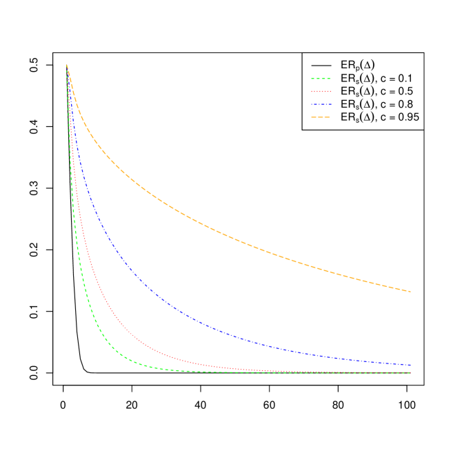
Figure 2: Error rates $ER_{p}(\Delta)$ and $ER_{s}(\Delta)$ as functions of $\Delta$ for $c\in\{0.1,0.5,0.8,0.95\}$.

3.2 Finite-sample performance

In this section we present the results of the simulation study. The aim is to investigate how good the asymptotic distribution of a linear combination of the discriminant function coefficients $\hat{\theta}=\mathbf{l}^{T}\hat{\mathbf{a}}$ performs in the case of the finite dimension and of the finite sample size. For that reason we compare the asymptotic distribution of the standardized $\hat{\theta}$ as given in Theorem 4 to the corresponding exact distribution obtained as a kernel density approximation with the Eppanechnikov kernel applied to the simulated data from the standardized exact distribution which are generated following the stochastic representation of Corollary 1: (i) first, $\xi_{b},z_{0;b},u_{b}$ are sampled independently from the corresponding univariate distributions provided in Corollary 1; (ii) second, $\hat{\theta}_{b}$ is computed by using (11) and standardized after that as in Theorem 4; (iii) finally, the previous two steps are repeated for $b=1,...,B$ times to obtain a sample of size $B$. It is noted that $B$ could be large to ensure a good performance of the kernel density estimator.

In the simulation study, we take $\mathbf{l}=\mathbf{1}_{p}$ ($p$-dimensional vector of ones). The elements of $\bm{\mu}_{1}$ and $\bm{\mu}_{2}$ are drawn from the uniform distribution on $\left[-1,1\right]$ when $\gamma>0$, while the first ten elements of $\mbox{\boldmath$\mu$}_{1}$ and the last ten elements of $\mbox{\boldmath$\mu$}_{2}$ are generated from the uniform distribution on $\left[-1,1\right]$ and the rest of the components are taken to be zero when $\gamma=0$. We also take $\mathbf{\Sigma}$ as a diagonal matrix, where every element is uniformly distributed on $\left(0,1\right]$. The results are compared for several values of $c=\{0.1,0.5,0.8,0.95\}$ and the corresponding values of $p,n_{1},n_{2}$. Simulated data consist of $N=10^{5}$ independent repetitions. In both cases $\gamma=0$ and $\gamma>0$ we plot two asymptotic density functions to investigate how robust are the obtained results to the choice of $\gamma$.

In Figures 3-4, we present the results in the case of equal and large sample sizes (data are drawn with $\gamma=0$ in Figure 3 and with $\gamma>0$ in Figure 4), while the plots in Figure 5 correspond to the case of one small sample and one large sample. We observe that the impact of the incorrect specification of $\gamma$ is not large, while some deviations are observed in Figure 5 for small values of $c$. If $c$ increases, then the difference between the two asymptotic distributions becomes negligible. In contrast, larger differences between the asymptotic distributions and the finite-sample one are observed for $c=0.8$ and $c=0.95$ in all figures, although their sizes are relatively small even in such extreme case.

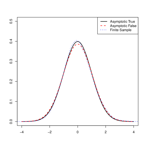
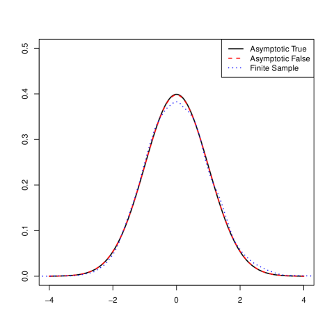
${a)\;\;p=50,~{}n_{1}=n_{2}=250}\hskip 115.0pt{b)\;\;p=250,~{}n_{1}=n_{2}=250}$

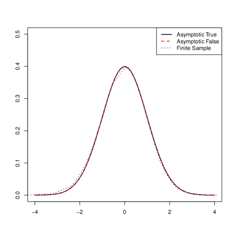
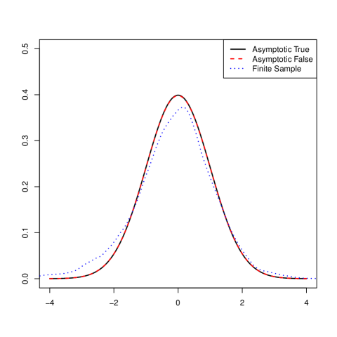
${c)\;\;p=400,~{}n_{1}=n_{2}=250}\hskip 115.0pt{d)\;\;p=475,~{}n_{1}=n_{2}=250}$

Figure 3: The kernel density estimator of the asymptotic distribution and standard normal for $\hat{\theta}$ as given in Theorem 4 for $\gamma=0$ and $c=\{0.1,0.5,0.8,0.95\}$.

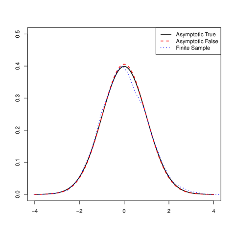
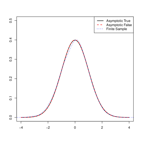
${a)\;\;p=50,~{}n_{1}=n_{2}=250}\hskip 115.0pt{b)\;\;p=250,~{}n_{1}=n_{2}=250}$

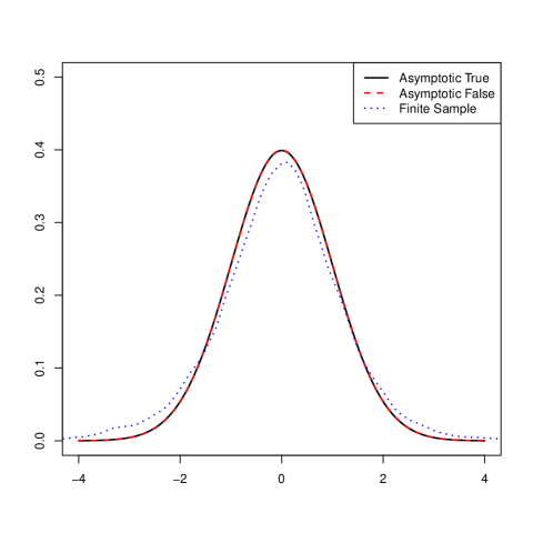
${c)\;\;p=400,~{}n_{1}=n_{2}=250}\hskip 115.0pt{d)\;\;p=475,~{}n_{1}=n_{2}=250}$

Figure 4: The kernel density estimator of the asymptotic distribution and standard normal for $\hat{\theta}$ as given in Theorem 4 for $\gamma>0$ and $c=\{0.1,0.5,0.8,0.95\}$.

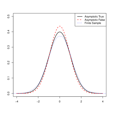
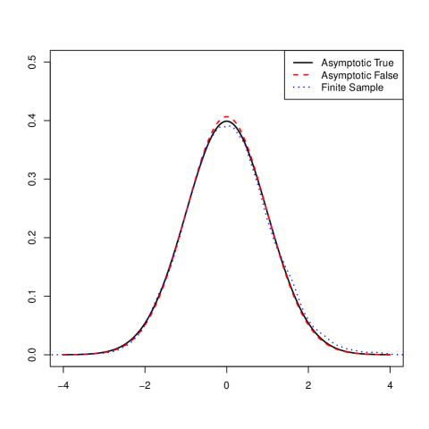
${a)\;\;p=50,~{}n_{1}=25,~{}n_{2}=475}\hskip 115.0pt{b)\;\;p=250,~{}n_{1}=25,~{}n_{2}=475}$

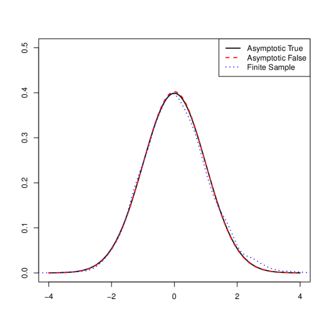
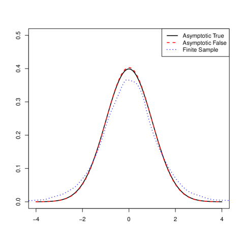
${c)\;\;p=400,~{}n_{1}=25,~{}n_{2}=475}\hskip 115.0pt{d)\;\;p=475,~{}n_{1}=25,~{}n_{2}=475}$

Figure 5: The kernel density estimator of the asymptotic distribution and standard normal for $\hat{\theta}$ as given in Theorem 4 for $\gamma>0$ and $c=\{0.1,0.5,0.8,0.95\}$.

References

- Agarwal et al., (2012) Agarwal, A., Negahban, S., and Wainwright, M. J. (2012). Noisy matrix decomposition via convex relaxation: Optimal rates in high dimensions. Annals of Statistics, 40(2):1171–1197.
- Bai et al., (2009) Bai, Z., Jiang, D., Yao, J.-F., and Zheng, S. (2009). Corrections to lrt on large-dimensional covariance matrix by rmt. Annals of Statistics, 37(6B):3822–3840.
- Bai and Silverstein, (2010) Bai, Z. and Silverstein, J. W. (2010). Spectral Analysis of Large Dimensional Random Matrices. New York, NY: Springer Science+ Business Media, LLC.
- Bickel and Levina, (2004) Bickel, P. J. and Levina, E. (2004). Some theory for fisher’s linear discriminant function,’naive bayes’, and some alternatives when there are many more variables than observations. Bernoulli, pages 989–1010.
- Bodnar et al., (2016) Bodnar, T., Gupta, A., and Parolya, N. (2016). Direct shrinkage estimation of large dimensional precision matrix. Journal of Multivariate Analysis, 146:223–236.
- Bodnar et al., (2014) Bodnar, T., Gupta, A. K., and Parolya, N. (2014). On the strong convergence of the optimal linear shrinkage estimator for large dimensional covariance matrix. Journal of Multivariate Analysis, 132:215–228.
- (7) Bodnar, T., Mazur, S., and Okhrin, Y. (2017a). Bayesian estimation of the global minimum variance portfolio. European Journal of Operational Research, 256:292–307.
- (8) Bodnar, T., Mazur, S., and Parolya, N. (2017b). Central limit theorems for functionals of large dimensional sample covariance matrix and mean vector in matrix-variate skewed model. Scandinavian Journal of Statistics, under revision.
- Bodnar and Okhrin, (2008) Bodnar, T. and Okhrin, Y. (2008). Properties of the singular, inverse and generalized inverse partitioned wishart distributions. Journal of Multivariate Analysis, 99:2389– 2405.
- Bodnar and Okhrin, (2011) Bodnar, T. and Okhrin, Y. (2011). On the product of inverse wishart and normal distributions with applications to discriminant analysis and portfolio theory. Scandinavian Journal of Statistics, 38(2):311–331.
- Bodnar and Reiß, (2016) Bodnar, T. and Reiß, M. (2016). Exact and asymptotic tests on a factor model in low and large dimensions with applications. Journal of Multivariate Analysis, 150:125–151.
- Bodnar and Schmid, (2008) Bodnar, T. and Schmid, W. (2008). A test for the weights of the global minimum variance portfolio in an elliptical model. Metrika, 67(2):127–143.
- (13) Cai, T. and Liu, W. (2011a). Adaptive thresholding for sparse covariance matrix estimation. Journal of the American Statistical Association, 106(494):672–684.
- (14) Cai, T. and Liu, W. (2011b). A direct estimation approach to sparse linear discriminant analysis. Journal of the American Statistical Association, 106(496):1566–1577.
- Cai et al., (2011) Cai, T., Liu, W., and Luo, X. (2011). A constrained minimization approach to sparse precision matrix estimation. Journal of the American Statistical Association, 106(494):594–607.
- Cai and Jiang, (2011) Cai, T. T. and Jiang, T. (2011). Limiting laws of coherence of random matrices with applications to testing covariance structure and construction of compressed sensing matrices. Annals of Statistics, 39(3):1496–1525.
- Chen et al., (2010) Chen, S. X., Zhang, L.-X., and Zhong, P.-S. (2010). Tests for high-dimensional covariance matrices. Journal of the American Statistical Association, 105(490):810–819.
- DasGupta, (2008) DasGupta, A. (2008). Asymptotic theory of statistics and probability. Springer Science & Business Media.
- Fan et al., (2008) Fan, J., Fan, Y., and Lv, J. (2008). High dimensional covariance matrix estimation using a factor model. Journal of Econometrics, 147(1):186–197.
- Fan et al., (2013) Fan, J., Liao, Y., and Mincheva, M. (2013). Large covariance estimation by thresholding principal orthogonal complements. Journal of the Royal Statistical Society: Series B (Statistical Methodology), 75(4):603–680.
- Fujikoshi and Seo, (1997) Fujikoshi, Y. and Seo, T. (1997). Asymptotic aproximations for epmc’s of the linear and the quadratic discriminant functions when the sample sizes and the dimension are large. Random operators and stochastic equations, University of Toronto.
- Givens and Hoeting, (2012) Givens, G. H. and Hoeting, J. A. (2012). Computational statistics. John Wiley & Sons.
- Gupta and Nagar, (2000) Gupta, A. and Nagar, D. (2000). Matrix Variate Distributions. Chapman and Hall/CRC, Boca Raton.
- Gupta et al., (2013) Gupta, A., Varga, T., and Bodnar, T. (2013). Elliptically contoured models in statistics and portfolio theory. Springer, second edition.
- Gupta and Bodnar, (2014) Gupta, A. K. and Bodnar, T. (2014). An exact test about the covariance matrix. Journal of Multivariate Analysis, 125:176–189.
- Jiang and Yang, (2013) Jiang, T. and Yang, F. (2013). Central limit theorems for classical likelihood ratio tests for high-dimensional normal distributions. Annals of Statistics, 41(4):2029–2074.
- Johnson et al., (2007) Johnson, R. A., Wichern, D. W., et al. (2007). Applied multivariate statistical analysis. Prentice hall Upper Saddle River, NJ.
- Johnstone, (2001) Johnstone, I. M. (2001). On the distribution of the largest eigenvalue in principal components analysis. Annals of Statistics, 29(2):295–327.
- Ledoit and Wolf, (2003) Ledoit, O. and Wolf, M. (2003). Improved estimation of the covariance matrix of stock returns with an application to portfolio selection. Journal of Empirical Finance, 10(5):603–621.
- Mathai and Provost, (1992) Mathai, A. and Provost, S. B. (1992). Quadratic Forms in Random Variables. Marcel Dekker.
- Muirhead, (1982) Muirhead, R. J. (1982). Aspects of Multivariate Statistical Theory. Wiley, New York.
- Narsky and Porter, (2013) Narsky, I. and Porter, F. C. (2013). Linear and quadratic discriminant analysis, logistic regression, and partial least squares regression. Statistical Analysis Techniques in Particle Physics: Fits, Density Estimation and Supervised Learning, pages 221–249.
- Rencher, (1998) Rencher, A. C. (1998). Multivariate statistical inference and applications, volume 338. Wiley-Interscience.
- Rencher and Christensen, (2012) Rencher, A. C. and Christensen, W. F. (2012). Methods of multivariate analysis. John Wiley & Sons.
- Shao et al., (2011) Shao, J., Wang, Y., Deng, X., Wang, S., et al. (2011). Sparse linear discriminant analysis by thresholding for high dimensional data. The Annals of statistics, 39(2):1241–1265.
- Srivastava and Kubokawa, (2007) Srivastava, M. S. and Kubokawa, T. (2007). Comparison of discrimination methods for high dimensional data. Journal of the Japan Statistical Society, 37:123–134.
- Tamatani, (2015) Tamatani, M. (2015). Asymptotic theory for discriminant analysis in high dimension low sample size. Memoirs of the Graduate School of Science and Engineering, Shimane University. Series B, Mathematics, pages 15–26.
- Wyman et al., (1990) Wyman, F. J., Young, D. M., and Turner, D. W. (1990). A comparison of asymptotic error rate expansions for the sample linear discriminant function. Pattern Recognition, 23:775–783.