“Convex Until Proven Guilty”: Dimension-Free Acceleration of Gradient Descent on Non-Convex Functions
Abstract
We develop and analyze a variant of Nesterov’s accelerated gradient descent (AGD) for minimization of smooth non-convex functions. We prove that one of two cases occurs: either our AGD variant converges quickly, as if the function was convex, or we produce a certificate that the function is “guilty” of being non-convex. This non-convexity certificate allows us to exploit negative curvature and obtain deterministic, dimension-free acceleration of convergence for non-convex functions. For a function with Lipschitz continuous gradient and Hessian, we compute a point with in gradient and function evaluations. Assuming additionally that the third derivative is Lipschitz, we require only evaluations.
1 Introduction
Nesterov’s seminal 1983 accelerated gradient method has inspired substantial development of first-order methods for large-scale convex optimization. In recent years, machine learning and statistics have seen a shift toward large scale non-convex problems, including methods for matrix completion Koren et al. (2009), phase retrieval Candès et al. (2015); Wang et al. (2016), dictionary learning Mairal et al. (2008), and neural network training LeCun et al. (2015). In practice, techniques from accelerated gradient methods—namely, momentum—can have substantial benefits for stochastic gradient methods, for example, in training neural networks Rumelhart et al. (1986); Kingma and Ba (2015). Yet little of the rich theory of acceleration for convex optimization is known to transfer into non-convex optimization.
Optimization becomes more difficult without convexity, as gradients no longer provide global information about the function. Even determining if a stationary point is a local minimum is (generally) NP-hard Murty and Kabadi (1987); Nesterov (2000). It is, however, possible to leverage non-convexity to improve objectives in smooth optimization: moving in directions of negative curvature can guarantee function value reduction. We explore the interplay between negative curvature, smoothness, and acceleration techniques, showing how an understanding of the three simultaneously yields a method that provably accelerates convergence of gradient descent for a broad class of non-convex functions.
1.1 Problem setting
We consider the unconstrained minimization problem
| (1) |
where is smooth but potentially non-convex. We assume throughout the paper that is bounded from below, two-times differentiable, and has Lipschitz continuous gradient and Hessian. In Section 4 we strengthen our results under the additional assumption that has Lipschitz continuous third derivatives. Following the standard first-order oracle model Nemirovski and Yudin (1983), we consider optimization methods that access only values and gradients of (and not higher order derivatives), and we measure their complexity by the total number of gradient and function evaluations.
Approximating the global minimum of to -accuracy is generally intractable, requiring time exponential in (Nemirovski and Yudin, 1983, §1.6). Instead, we seek a point that is -approximately stationary, that is,
| (2) |
Finding stationary points is a canonical problem in nonlinear optimization Nocedal and Wright (2006), and while saddle points and local maxima are stationary, excepting pathological cases, descent methods that converge to a stationary point converge to a local minimum (Lee et al., 2016; Nemirovski, 1999, §3.2.2).
If we assume is convex, gradient descent satisfies the bound (2) after gradient evaluations, and AGD improves this rate to Nesterov (2012). Without convexity, gradient descent is significantly worse, having worst-case complexity Cartis et al. (2010). More sophisticated gradient-based methods, including nonlinear conjugate gradient Hager and Zhang (2006) and L-BFGS Liu and Nocedal (1989) provide excellent practical performance, but their global convergence guarantees are no better than . Our work Carmon et al. (2016) and, independently, Agarwal et al. (2016), break this barrier, obtaining the rate . Before we discuss this line of work in Section 1.3, we overview our contributions.
1.2 Our contributions
“Convex until proven guilty”
Underpinning our results is the observation that when we run Nesterov’s accelerated gradient descent (AGD) on any smooth function , one of two outcomes must follow:
-
(a)
AGD behaves as though was -strongly convex, satisfying inequality (2) in iterations.
-
(b)
There exist points in the AGD trajectory that prove is “guilty” of not being -strongly convex,
(3)
The intuition behind these observations is that if inequality (3) never holds during the iterations of AGD, then “looks” strongly convex, and the convergence (a) follows. In Section 2 we make this observation precise, presenting an algorithm to monitor AGD and quickly find the witness pair satisfying (3) whenever AGD progresses more slowly than it does on strongly convex functions. We believe there is potential to apply this strategy beyond AGD, extending additional convex gradient methods to non-convex settings.
An accelerated non-convex gradient method
In Section 3 we propose a method that iteratively applies our monitored AGD algorithm to augmented by a proximal regularizer. We show that both outcomes (a) and (b) above imply progress minimizing , where in case (b) we make explicit use of the negative curvature that AGD exposes. These progress guarantees translate to an overall first-order oracle complexity of , a strict improvement over the rate of gradient descent. In Section 5 we report preliminary experimental results, showing a basic implementation of our method outperforms gradient descent but not nonlinear conjugate gradient.
Improved guarantees with third-order smoothness
As we show in Section 4, assuming Lipschitz continuous third derivatives instead of Lipschitz continuous Hessian allows us to increase the step size we take when exploiting negative curvature, making more function progress. Consequently, the complexity of our method improves to . While the analysis of the third-order setting is more complex, the method remains essentially unchanged. In particular, we still use only first-order information, never computing higher-order derivatives.
1.3 Related work
Nesterov and Polyak (2006) show that cubic regularization of Newton’s method finds a point that satisfies the stationarity condition (2) in evaluations of the Hessian. Given sufficiently accurate arithmetic operations, a Lipschitz continuous Hessian is approximable to arbitrary precision using finite gradient differences, and obtaining a full Hessian requires gradient evaluations. A direct implementation of the Nesterov-Polyak method with a first-order oracle therefore has gradient evaluation complexity , improving on gradient descent only if , which may fail in high-dimensions.
In two recent papers, we (Carmon et al., 2016) and (independently) Agarwal et al. obtain better rates for first-order methods. Agarwal et al. (2016) propose a careful implementation of the Nesterov-Polyak method, using accelerated methods for fast approximate matrix inversion. In our earlier work, we employ a combination of (regularized) accelerated gradient descent and the Lanczos method. Both find a point that satisfies the bound (2) with probability at least using gradient and Hessian-vector product evaluations.
The primary conceptual difference between our approach and those of Carmon et al. and Agarwal et al. is that we perform no eigenvector search: we automatically find directions of negative curvature whenever AGD proves “guilty” of non-convexity. Qualitatively, this shows that explicit second orders information is unnecessary to improve upon gradient descent for stationary point computation. Quantitatively, this leads to the following improvements:
-
(i)
Our result is dimension-free and deterministic, with complexity independent of the ratio , compared to the dependence of previous works. This is significant, as may be comparable to , making it unclear whether the previous guarantees are actually better than those of gradient descent.
-
(ii)
Our method uses only gradient evaluations, and does not require Hessian-vector products. In practice, Hessian-vector products may be difficult to implement and more expensive to compute than gradients.
-
(iii)
Under third-order smoothness assumptions we improve our method to achieve rate. It is unclear how to extend previous approaches to obtain similar guarantees.
In distinction from the methods of Carmon et al. (2016) and Agarwal et al. (2016), our method provides no guarantees on positive definiteness of ; if initialized at a saddle point it will terminate immediately. However, as we further explain in Section C, we may combine our method with a fast eigenvector search to recover the approximate positive definiteness guarantee , even improving it to using third-order smoothness, but at the cost of reintroducing randomization, Hessian-vector products and a complexity term.
1.4 Preliminaries and notation
Here we introduce notation and briefly overview definitions and results we use throughout. We index sequences by subscripts, and use as shorthand for . We use and to denote points in . Additionally, denotes step sizes, denote desired accuracy, denotes a scalar and denotes the Euclidean norm on . We denote the th derivative of a function by . We let .
A function has -Lipschitz th derivative if it is times differentiable and for every and unit vector , the one-dimensional function satisfies
We refer to this property as th-order smoothness, or simply smoothness for , where it coincides with the Lipschitz continuity of . Throughout the paper, we make extensive use of the well-known consequence of Taylor’s theorem, that the Lipschitz constant of the th-order derivative controls the error in the th order Taylor series expansion of , i.e. for we have
| (4) |
A function is -strongly convex if for all .
2 Algorithm components
We begin our development by presenting the two building blocks of our result: a monitored variation of AGD (Section 2.1) and a negative curvature descent step (Section 2.2) that we use when the monitored version of AGD certifies non-convexity. In Section 3, we combine these components to obtain an accelerated method for non-convex functions.
2.1 AGD as a convexity monitor
The main component in our approach is Alg. 1, AGD-until-proven-guilty. We take as input an -smooth function , conjectured to be -strongly convex, and optimize it with Nesterov’s accelerated gradient descent method for strongly convex functions (lines 3 and 4). At every iteration, the method invokes Certify-progress to test whether the optimization is progressing as it should for strongly convex functions, and in particular that the gradient norm is decreasing exponentially quickly (line 5). If the test fails, Find-witness-pair produces points proving that violates -strong convexity. Otherwise, we proceed until we find a point such that .
The efficacy of our method is based on the following guarantee on the performance of AGD.
Proposition 1.
Let be -smooth, and let and be the sequence of iterates generated by AGD-until-proven-guilty(, , , , ) for some and . Fix . If for we have
| (5) |
for both and , then
| (6) |
where and .
Proposition 1 is essentially a restatement of established results (Nesterov, 2004; Bubeck, 2014), where we take care to phrase the requirements on in terms of local inequalities, rather than a global strong convexity assumption. For completeness, we provide a proof of Proposition 1 in Section A.1.
Corollary 1.
Let be -smooth, let , and . Let AGD-until-proven-guilty(, , , , ). Then the number of iterations satisfies
| (7) |
where is as in line 4 of Certify-progress. If (non-convexity was detected), then
| (8) |
where for some and or (defined on line 5 of AGD-until-proven-guilty). Moreover,
| (9) |
Proof.
The bound (7) is clear for . For , the algorithm has not terminated at iteration , and so we know that neither the condition in line 9 of AGD-until-proven-guilty nor the condition in line 5 of Certify-progress held at iteration . Thus
which gives the bound (7) when rearranged.
Now we consider the returned vectors , , , and from AGD-until-proven-guilty. Note that only if . Suppose that , then by line 2 of Certify-progress we have,
since . Since this contradicts the progress bound (6), we obtain the certificate (8) by the contrapositive of Proposition 1: condition (5) must not hold for some , implying Find-witness-pair will return for some .
Similarly, if then by line 5 of Certify-progress we must have
Since is -smooth we have the standard progress guarantee (c.f. Nesterov (2004) §1.2.3) , again contradicting inequality (6).
To see that the bound (9) holds, note that for since condition 2 of Certify-progress did not hold. If for some then holds trivially. Alternatively, if then condition 2 did not hold at time as well, so we have and also as noted above; therefore . ∎
Before continuing, we make two remarks about implementation of Alg. 1.
-
(1)
As stated, the algorithm requires evaluation of two function gradients per iteration (at and ). Corollary 1 holds essentially unchanged if we execute line 9 of AGD-until-proven-guilty and lines 3-5 of Certify-progress only once every iterations, where is some fixed number (say 10). This reduces the number of gradient evaluations to per iteration.
-
(2)
Direct implementation would require memory to store the sequences , and for later use by Find-witness-pair. Alternatively, Find-witness-pair can regenerate these sequences from their recursive definition while iterating over , reducing the memory requirement to and increasing the number of gradient and function evaluations by at most a factor of 2.
In addition, while our emphasis is on applying AGD-until-proven-guilty to non-convex problems, the algorithm has implications for convex optimization. For example, we rarely know the strong convexity parameter of a given function ; to remedy this, O’Donoghue and Candès (2015) propose adaptive restart schemes. Instead, one may repeatedly apply AGD-until-proven-guilty and use the witnesses to update .
2.2 Using negative curvature
The second component of our approach is exploitation of negative curvature to decrease function values; in Section 3 we use AGD-until-proven-guilty to generate such that
| (10) |
a nontrivial violation of convexity (where is a parameter we control using a proximal term). By taking an appropriately sized step from in the direction , Alg. 2 can substantially lower the function value near whenever the convexity violation (10) holds. The following basic lemma shows this essential progress guarantee.
Lemma 1.
Let have -Lipschitz Hessian. Let and let and satisfy (10). If , then for every , Exploit-NC-pair() finds a point such that
| (11) |
Proof.
We proceed in two parts; in the first part, we show that has negative curvature of at least in the direction at the point . We then show that this negative curvature guarantees a gradient step with magnitude produces the required progress in function value.
Defining , we obtain
where inequality follows by assumption (10). Let . Using that , we substitute for the integrand to find that , and using the Lipschitz continuity of yields
| (12) |
where we have used that by assumption.
3 Accelerating non-convex optimization
We now combine the accelerated convergence guarantee of Corollary 1 and the non-convex progress guarantee of Lemma 1 to form Guarded-non-convex-AGD. The idea for the algorithm is as follows. Consider iterate , denoted . We create a proximal function by adding the proximal term to . Applying AGD-until-proven-guilty to yields the sequences , and possibly a non-convexity witnessing pair (line 3). If are not available, we set and continue to the next iteration. Otherwise, by Corollary 1, and certify that is not strongly convex, and therefore that has negative curvature. Exploit-NC-pair then leverages this negative curvature, obtaining a point . The next iterate is the best out of and in terms of function value.
The following central lemma provides a progress guarantee for each of the iterations of Alg. 3.
Lemma 2.
Let be -smooth and have -Lipschitz continuous Hessian, let and . Let be the iterates Guarded-non-convex-AGD(, , , , , ) generates. Then for each ,
| (13) |
Proof.
Fix an iterate index ; throughout the proof we let and refer to outputs of AGD-until-proven-guilty in the th iteration. We consider the cases and separately. In the former case, standard proximal point arguments suffice, while in the latter case we require more care.
The simpler case is (no convexity violation detected), in which and (since AGD-until-proven-guilty terminated on line 9). Moreover, implies that Guarded-non-convex-AGD does not terminate at iteration , and therefore . Consequently,
The case also implies , as the condition in line 2 of Certify-progress never holds, and therefore
which establishes the claim in the case .
Now we consider the case (non-convexity detected). By Corollary 1,
| (14) |
By definition of , we have for any that
where the inequality is Eq. (14). Therefore, we conclude that inequality (10) must hold. To apply Lemma 1, we must control the distance between and . We present the following lemma, which shows how acts as an insurance policy against growing too large.
Lemma 3.
Let be -smooth, and . At any iteration of Guarded-non-convex-AGD, if and the best iterate satisfies then for ,
Deferring the proof of Lemma 3 briefly, we show how it yields Lemma 2. We set and consider two cases. First, if
then we are done, since . In the converse case, if , Lemma 3 implies . Therefore, we can exploit the negative curvature in , as Lemma 1 guarantees (with ),
Here inequality uses that by Corollary 1. This implies inequality (13) holds and concludes the case . ∎
Proof of Lemma 3. We begin by noting that for by Corollary 1. Using we therefore have
which implies . By Corollary 1 we also have , so we similarly obtain . Using , where , we have by the triangle inequality that
for every . Finally, since for some , this gives the last inequality of the lemma, as
.
∎
Lemma 2 shows we can accelerate gradient descent in a non-convex setting. Indeed, ignoring all problem-dependent constants, setting in the bound (13) shows that we make progress at every iteration of Guarded-non-convex-AGD, and consequently the number of iterations is bounded by . Arguing that calls to AGD-until-proven-guilty each require gradient computations yields the following complexity guarantee.
Theorem 1.
Let be -smooth and have -Lipschitz continuous Hessian. Let , and . Set
| (15) |
then Guarded-non-convex-AGD(, , , , , ) finds a point such that with at most
| (16) |
gradient evaluations.
Proof.
We bound two quantities: the number of calls to AGD-until-proven-guilty, which we denote by , and the maximum number of steps AGD-until-proven-guilty performs when it is called, which we denote by . The overall number gradient evaluations is , as we compute at most gradients per iterations (at the points and ).
The upper bound on is immediate from Lemma 2, as by telescoping the progress guarantee (13) we obtain
where the final inequality follows by substituting our choice (15), of . We conclude that
| (17) |
To bound the number of steps of AGD-until-proven-guilty, note that for every
Therefore, substituting , and into the guarantee (7) of Corollary 1,
| (18) |
We conclude this section with two brief remarks.
-
(1)
The conditions on guarantee that the bound (16) is non-trivial. If , then gradient descent achieves better guarantees. Indeed, with step-size , gradient descent satisfies within at most iterations (cf. Nesterov, 2004, Eq. 1.2.13). Substituting therefore yields
Alternatively, if then we have by inequality (17) that , so Alg. 3 halts after at most a single iteration. Nevertheless, the bounds (17) and (18) hold for any .
-
(2)
While we state Theorem 1 in terms of gradient evaluation count, a similar bound holds for function evaluations as well. Indeed, inspection of our method reveals that each iteration of Alg. 3 evaluates the function and not the gradient at at most the three points and ; both complexity measures are therefore of the same order.
4 Incorporating third-order smoothness
In this section, we show that when third-order derivatives are Lipschitz continuous, we can improve the convergence rate of Alg. 3 by modifying two of its subroutines. In Section 4.1 we introduce a modified version of Exploit-NC-pair that can decrease function values further using third-order smoothness. In Section 4.2 we change Find-best-iterate to provide a guarantee that is never too large. We combine these two results in Section 4.3 and present our improved complexity bounds.
4.1 Making better use of negative curvature
Our first observation is that third-order smoothness allows us to take larger steps and make greater progress when exploiting negative curvature, as the next lemma formalizes.
Lemma 4.
Let have -Lipschitz third-order derivatives, , and be a unit vector. If then, for every ,
| (19) |
Proof.
For , define . By assumption is -Lipschitz continuous, and therefore
Set and set . As , we have
the last inequality using , and . That gives the result. ∎
Comparing Lemma 4 to the second part of the proof of Lemma 1, we see that second-order smoothness with optimal guarantees function decrease, while third-order smoothness guarantees a decrease. Recalling Theorem 1, where scales as a power of , this is evidently a significant improvement. Additionally, this benefit is essentially free: there is no increase in computational cost and no access to higher order derivatives. Examining the proof, we see that the result is rooted in the anti-symmetry of the odd-order terms in the Taylor expansion. This rules out extending this idea to higher orders of smoothness, as they contain symmetric fourth order terms.
Extending this insight to the setting of Lemma 1 is complicated by the fact that, at relevant scales of , it is no longer possible to guarantee that there is negative curvature at either or . Nevertheless, we are able to show that a small modification of Exploit-NC-pair achieves the required progress.
Lemma 5.
Let have -Lipschitz third-order derivatives. Let and let and satisfy (10) and let . Then for every , Exploit-NC-pair3() finds a point such that
| (20) |
4.2 Bounding the function values of the iterates using cubic interpolation
An important difference between Lemmas 1 and 5 is that the former guarantees lower objective value than , while the latter only improves . We invoke these lemmas for for some produced by AGD-until-proven-guilty, but Corollary 1 only bounds the function value at and ; might be much larger than , rendering the progress guaranteed by Lemma 5 useless. Fortunately, we are able show that whenever this happens, there must be a point on the line that connects and for which the function value is much lower than . We take advantage of this fact in Alg. 5, where we modify Find-best-iterate to consider additional points, so that whenever the iterate it finds is not much better than , then is guaranteed to be close to . We formalize this claim in the following lemma, which we prove in Section B.2.
Lemma 6.
Let be -smooth and have -Lipschitz continuous third-order derivatives, and let with . Consider Guarded-non-convex-AGD with Find-best-iterate replaced by Find-best-iterate3. At any iteration, if and the best iterate satisfies then,
We now explain the idea behind the proof of Lemma 6. Let be such that (such always exists by Corollary 1). If then and the result is trivial, so we assume . Let be the restriction of to the line containing and (and also and ). Suppose now that is a cubic polynomial. Then, it is completely determined by its values at any 4 points, and for independent of . By substituting the bounds and , we obtain an upper bound on when is cubic. To generalize this upper bound to with Lipschitz third-order derivative, we can simply add to it the approximation error of an appropriate third-order Taylor series expansion, which is bounded by a term proportional to .
4.3 An improved rate of convergence
With our algorithmic and analytic upgrades established, we are ready to state the enhanced performance guarantees for Guarded-non-convex-AGD, where from here on we assume that Exploit-NC-pair3 and Find-best-iterate3 subsume Exploit-NC-pair and Find-best-iterate, respectively.
Lemma 7.
Let be -smooth and have -Lipschitz continuous third-order derivatives, let and . If is the sequence of iterates produced by Guarded-non-convex-AGD(, , , , , ), then for every ,
| (21) |
The proof of Lemma 7 is essentially identical to the proof of Lemma 2, where we replace Lemma 1 with Lemmas 5 and 6 and set . For completeness, we give a full proof in Section B.3. The gradient evaluation complexity guarantee for third-order smoothness then follows precisely as in our proof of Theorem 1; see Sec. B.4 for a proof of the following
Theorem 2.
Let be -smooth and have -Lipschitz continuous third-order derivatives. Let , and . If we set
| (22) |
Guarded-non-convex-AGD(, , , , , ) finds a point such that and requires at most
| (23) |
gradient evaluations.
While achieving the guarantees that Theorem 2 provides requires some modification of our algorithms, these do not come at the expense of the convergence guarantees of Theorem 1 when we have only second order smoothness. That is, the results of Theorem 1 remain valid even with the algorithmic modifications of this section, and Alg. 3 transitions between smoothness regimes by varying the scaling of and with .
5 Preliminary experiments
The primary purpose of this paper is to demonstrate the feasibility of acceleration for non-convex problems using only first-order information. Given the long history of development of careful schemes for non-linear optimization, it is unrealistic to expect a simple implementation of the momentum-based Algorithm 3 to outperform state-of-the-art methods such as non-linear conjugate gradients and L-BFGS. It is important, however, to understand the degree of non-convexity in problems we encounter in practice, and to investigate the efficacy of the negative curvature detection-and-exploitation scheme we propose.
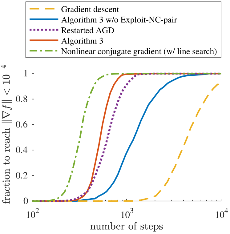
Toward this end, we present two experiments: (1) fitting a non-linear regression model and (2) training a small neural network. In these experiments we compare a basic implementation of Alg. 3 with a number baseline optimization methods: gradient descent (GD), non-linear conjugate gradients (NCG) Hager and Zhang (2006), Accelerated Gradient Descent (AGD) with adaptive restart O’Donoghue and Candès (2015) (RAGD), and a crippled version of Alg. 3 without negative curvature exploitation (C-Alg. 3). We compare the algorithms on the number of gradient steps, but note that the number of oracle queries per step varies between methods. We provide implementation details in Section D.1.
(a)
(b)
(c)
For our first experiment, we study robust linear regression with the smooth biweight loss Beaton and Tukey (1974),
The function is a robust modification of the quadratic loss; it is approximately quadratic for small errors, but insensitive to larger errors. For 1,000 independent experiments, we randomly generate problem data to create a highly non-convex problem as follows. We set and , and we draw . We generate as follows. We first draw a “ground truth” vector . We then set , where and the elements of are i.i.d. Bernoulli. These parameters make the problem substantially non-convex.
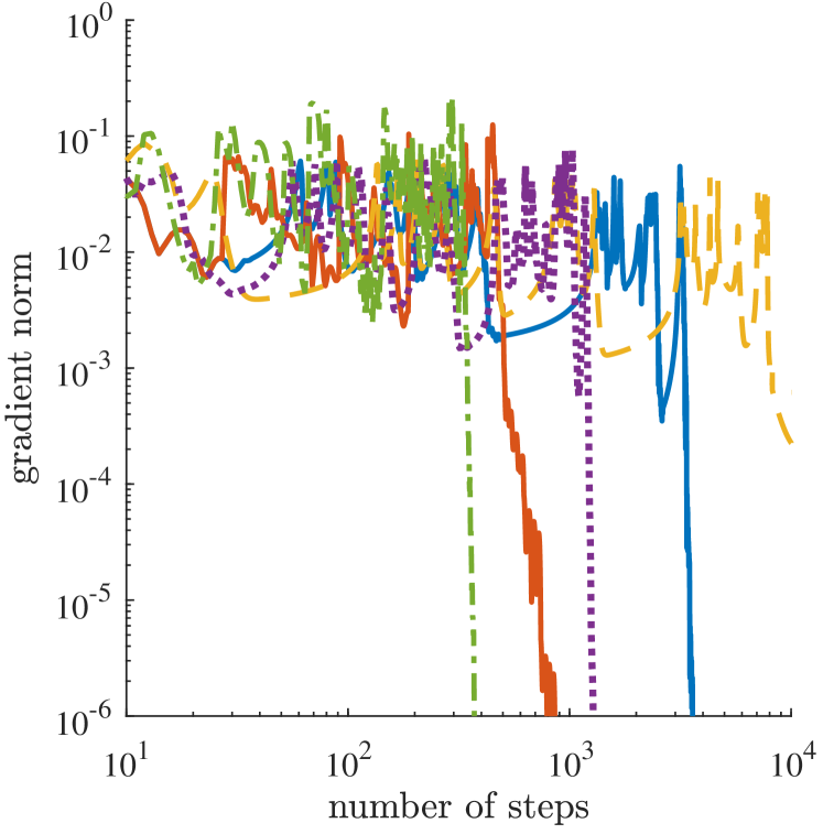
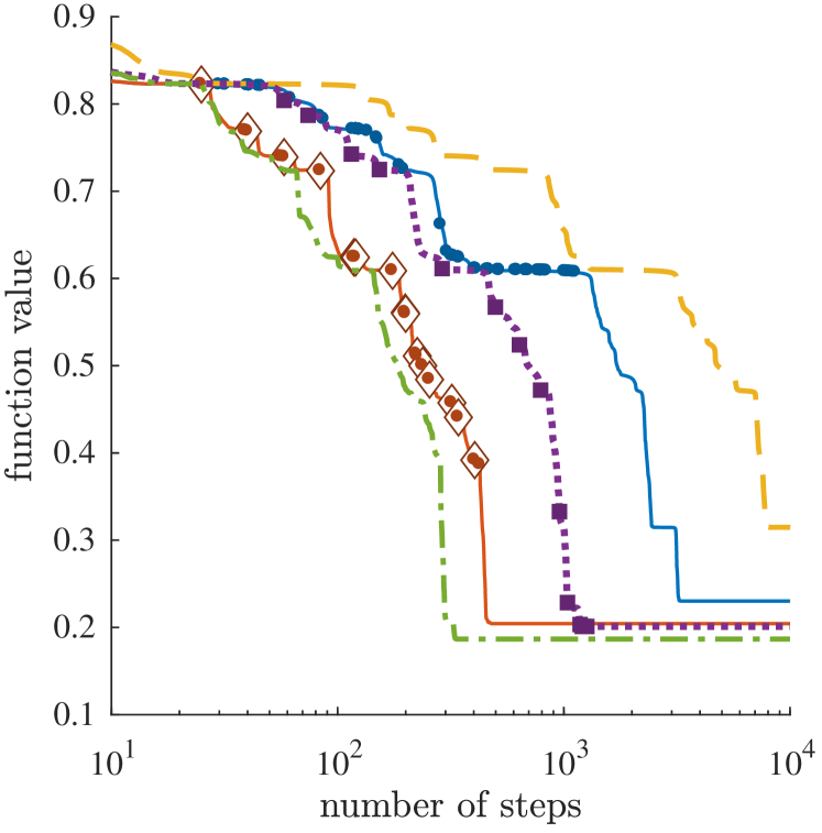
In Figure 1 we plot aggregate convergence time statistics, as well as gradient norm and function value trajectories for a single representative problem instance. The figure shows that gradient descent and C-Alg. 3 (which does not exploit curvature) converge more slowly than the other methods. When C-Alg. 3 stalls it is detecting negative curvature, which implies the stalling occurs around saddle points. When negative curvature exploitation is enabled, Alg. 3 is faster than RAGD, but slower than NCG. In this highly non-convex problem, different methods often converge to local minima with (sometimes significantly) different function values. However, each method found the “best” local minimum in a similar fraction of the generated instances, so there does not appear to be a significant difference in the ability of the methods to find “good” local minima in this problem ensemble.
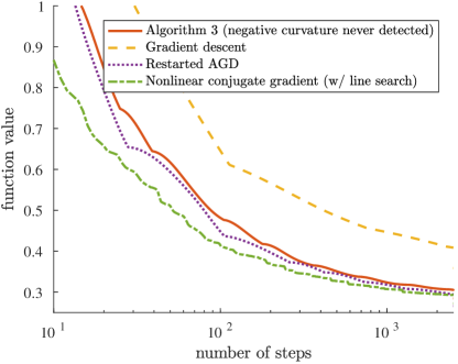
For the second experiment we fit a neural network model111Our approach in its current form is inapplicable to training neural networks of modern scale, as it requires computation of exact gradients. comprising three fully-connected hidden layers containing , and units, respectively, on the MNIST handwritten digits dataset LeCun et al. (1998) (see Section D.2). Figure 2 shows a substantial performance gap between gradient descent and the other methods, including Alg. 3. However, this is not due to negative curvature exploitation; in fact, Alg. 3 never detects negative curvature in this problem, implying AGD never stalls. Moreover, RAGD never restarts. This suggests that the loss function is “effectively convex” in large portions of the training trajectory, consistent with the empirical observations of Goodfellow et al. (2015); this phenomenon may merit further investigation.
We conclude that our approach can augment AGD in the presence of negative curvature, but that more work is necessary to make it competitive with established methods such as non-linear conjugate gradients. For example, adaptive schemes for setting and must be developed. However, the success of our method may depend on whether AGD stalls at all in real applications of non-convex optimization.
Acknowledgment
OH was supported by the PACCAR INC fellowship. YC and JCD were partially supported by the SAIL-Toyota Center for AI Research and NSF-CAREER award 1553086. YC was partially supported by the Stanford Graduate Fellowship and the Numerical Technologies Fellowship.
References
- Agarwal et al. (2016) N. Agarwal, Z. Allen-Zhu, B. Bullins, E. Hazan, and T. Ma. Finding approximate local minima for nonconvex optimization in linear time. arXiv preprint arXiv:1611.01146, 2016.
- Beaton and Tukey (1974) A. E. Beaton and J. W. Tukey. The fitting of power series, meaning polynomials, illustrated on band-spectroscopic data. Technometrics, 16(2):147–185, 1974.
- Beck and Teboulle (2009) A. Beck and M. Teboulle. Gradient-based algorithms with applications to signal recovery. Convex optimization in signal processing and communications, pages 42–88, 2009.
- Bubeck (2014) S. Bubeck. Convex optimization: Algorithms and complexity. arXiv preprint arXiv:1405.4980, 2014.
- Candès et al. (2015) E. J. Candès, X. Li, and M. Soltanolkotabi. Phase retrieval via Wirtinger flow: Theory and algorithms. IEEE Transactions on Information Theory, 61(4):1985–2007, 2015.
- Carmon et al. (2016) Y. Carmon, J. C. Duchi, O. Hinder, and A. Sidford. Accelerated methods for non-convex optimization. arXiv preprint arXiv:1611.00756, 2016.
- Cartis et al. (2010) C. Cartis, N. I. Gould, and P. L. Toint. On the complexity of steepest descent, Newton’s and regularized Newton’s methods for nonconvex unconstrained optimization problems. SIAM journal on optimization, 20(6):2833–2852, 2010.
- Glorot and Bengio (2010) X. Glorot and Y. Bengio. Understanding the difficulty of training deep feedforward neural networks. In Aistats, volume 9, pages 249–256, 2010.
- Goodfellow et al. (2015) I. J. Goodfellow, O. Vinyals, and A. M. Saxe. Qualitatively characterizing neural network optimization problems. In International Conference on Learning Representations, 2015.
- Hager and Zhang (2006) W. W. Hager and H. Zhang. A survey of nonlinear conjugate gradient methods. Pacific Journal of Optimization, 2(1):35–58, 2006.
- Kingma and Ba (2015) D. Kingma and J. Ba. Adam: A method for stochastic optimization. In International Conference on Learning Representations, 2015.
- Koren et al. (2009) Y. Koren, R. Bell, and C. Volinsky. Matrix factorization techniques for recommender systems. Computer, 42(8), 2009.
- LeCun et al. (1998) Y. LeCun, C. Cortes, and C. J. Burges. The MNIST database of handwritten digits, 1998.
- LeCun et al. (2015) Y. LeCun, Y. Bengio, and G. Hinton. Deep learning. Nature, 521(7553):436–444, 2015.
- Lee et al. (2016) J. D. Lee, M. Simchowitz, M. I. Jordan, and B. Recht. Gradient descent only converges to minimizers. In 29th Annual Conference on Learning Theory (COLT), pages 1246—1257, 2016.
- Liu and Nocedal (1989) D. C. Liu and J. Nocedal. On the limited memory BFGS method for large scale optimization. Mathematical Programming, 45(1):503–528, 1989.
- Mairal et al. (2008) J. Mairal, F. Bach, J. Ponce, G. Sapiro, and A. Zisserman. Supervised dictionary learning. In Advances in Neural Information Processing Systems 21, 2008.
- Murty and Kabadi (1987) K. Murty and S. Kabadi. Some NP-complete problems in quadratic and nonlinear programming. Mathematical Programming, 39:117–129, 1987.
- Nemirovski (1999) A. Nemirovski. Optimization II: Standard numerical methods for nonlinear continuous optimization. Technion – Israel Institute of Technology, 1999. URL http://www2.isye.gatech.edu/~nemirovs/Lect_OptII.pdf.
- Nemirovski and Yudin (1983) A. Nemirovski and D. Yudin. Problem Complexity and Method Efficiency in Optimization. Wiley, 1983.
- Nesterov (1983) Y. Nesterov. A method of solving a convex programming problem with convergence rate . Soviet Mathematics Doklady, 27(2):372–376, 1983.
- Nesterov (2000) Y. Nesterov. Squared functional systems and optimization problems. In High Performance Optimization, volume 33 of Applied Optimization, pages 405–440. Springer, 2000.
- Nesterov (2004) Y. Nesterov. Introductory Lectures on Convex Optimization. Kluwer Academic Publishers, 2004.
- Nesterov (2012) Y. Nesterov. How to make the gradients small. Optima 88, 2012.
- Nesterov and Polyak (2006) Y. Nesterov and B. T. Polyak. Cubic regularization of Newton method and its global performance. Mathematical Programming, 108(1):177–205, 2006.
- Nocedal and Wright (2006) J. Nocedal and S. J. Wright. Numerical Optimization. Springer, 2006.
- O’Donoghue and Candès (2015) B. O’Donoghue and E. Candès. Adaptive restart for accelerated gradient schemes. Foundations of Computational Mathematics, 15(3):715–732, 2015.
- Polak and Ribière (1969) E. Polak and G. Ribière. Note sur la convergence de directions conjugées. Rev. Fr. Inform. Rech. Oper. v16, pages 35–43, 1969.
- Rumelhart et al. (1986) D. E. Rumelhart, G. E. Hinton, and R. J. Williams. Learning internal representations by error propagation. In D. E. Rumelhart and J. L. McClelland, editors, Parallel Distributed Processing – Explorations in the Microstructure of Cognition, chapter 8, pages 318–362. MIT Press, 1986.
- Wang et al. (2016) G. Wang, G. B. Giannakis, and Y. C. Eldar. Solving systems of random quadratic equations via truncated amplitude flow. arXiv:1605.08285 [stat.ML], 2016.
Supplementary material
Appendix A Proofs from Section 2
A.1 Proof of Proposition 1
See 1
Proof.
The proof is closely based on the proof of Theorem 3.18 of Bubeck (2014), which itself is based on the estimate sequence technique of Nesterov (2004). We modify the proof slightly to avoid arguments that depend on the global minimum of . This enables using inequalities (5) to prove the result, instead of -strong convexity of the function .
We define -strongly convex quadratic functions by induction as
and, for ,
| (24) |
Using (5) with , straightforward induction shows that
| (25) |
We now prove (26) by induction. Note that it is true at since is the global minimizer of . We have,
where inequality (a) follows from the definition and the -smoothness of , inequality (b) is the induction hypothesis and inequality (c) is assumption (5) with .
Past this point the proof is identical to the proof of Theorem 3.18 of Bubeck (2014), but we continue for sake of completeness.
To complete the induction argument we now need to show that:
| (27) |
Note that (immediate by induction) and therefore
for some . By differentiating (24) and using the above form of we obtain
Since by definition , we have
| (28) |
Using (24), evaluating evaluating at gives,
| (29) |
Substituting (28) gives
which combined with (29) yields
Examining this equation, it is seen that implies (27) and therefore concludes the proof of Proposition 1. We establish the relation by induction,
where the first equality comes from (28), the second from the induction hypothesis, the third from the definition of and the last one from the definition of . ∎
Appendix B Proofs from Section 4
B.1 Proof of Lemma 5
We begin by proving the following normalized version of Lemma 5.
Lemma 8.
Let be thrice differentiable, be -Lipschitz continuous for some and let
| (30) |
for some . Then for any
| (31) |
where .
Proof.
Define
By the Lipschitz continuity of , we have that for any (see Section 1.4). Similarly, viewing as the first derivative of , we have and . The assumption (30) therefore implies,
| (32) |
It is also easy to verify that
Substituting into the definition of and rearranging, this yields
| (33) |
and
| (34) |
Suppose now that holds instead. By (33) and (32) we then have
where the equality follows from the definition . We lower bound as
where the first inequality follows from the fact that is monotonically decreasing in and the assumption . Noting that , we have the upper bound . Combining these bounds gives . Applying at and , and using and once more, we obtain,
| (36) |
∎
See 5
Proof.
Define
We have
Additionally, since has -Lipschitz third order derivatives, is Lipschitz continuous, so we may apply Lemma 8 at . Letting , we note that . Similarly, for we have with given in line 2 of Exploit-NC-pair3. The result is now immediate from (31), as
where in the last transition we have used . ∎
B.2 Proof of Lemma 6
We first state and prove a normalized version of the central argument in the proof of Lemma 6
Lemma 9.
Let be thrice differentiable and let be -Lipschitz continuous for some . If
| (37) |
for some , then
for any .
Proof.
Define
By the Lipschitz continuity of , we have that , for any . Using the expressions for at to eliminate and , we obtain:
Applying (37), and gives the required bound:
∎
We now prove Lemma 6 itself.
See 6
Proof.
Let be such that (such always exists by Corollary 1). If then and the result is trivial, so we assume . Let
Note that
where is defined in line 1 of AGD-until-proven-guilty, and we have used the guarantee from Corollary 1. Moreover, by the Lipschitz continuity of the third derivatives of , is -Lipschitz continuous. Therefore, we can apply Lemma 9 with and at and obtain
To complete the proof, we note that Lemma 3 guarantees and therefore
where we have used . ∎
B.3 Proof of Lemma 7
See 7
Proof.
Fix an iterate index ; throughout the proof we let and refer to outputs of AGD-until-proven-guilty in the th iteration. We consider only the case , as the argument for is unchanged from Lemma 2.
As argued in the proof of Lemma 2, when , condition (10) holds. We set and consider two cases. First, if then we are done, since . Second, if , by Lemma 3 we have that
Therefore, we can use Lemma 5 (with as defined above) to show that
| (38) |
By Corollary 1, . Moreover, since and , we may apply Lemma 6 to obtain
Combining this with (38), we find that
which concludes the case under third-order smoothness. ∎
B.4 Proof of Theorem 2
See 2
Proof.
The proof proceeds exactly like the proof of Theorem 1. As argued there, the number of gradient evaluations is at most , where is number of iterations of Guarded-non-convex-AGD and is the maximum amount of steps performed in any call to AGD-until-proven-guilty.
We derive the upper bound on directly from Lemma 7, as by telescoping (13) we obtain
where the last transition follows from substituting (22), our choice of . We therefore conclude that
| (39) |
Appendix C Adding a second-order guarantee
In this section, we sketch how to obtain simultaneous guarantees on the gradient and minimum eigenvalue of the Hessian. We use the notation to hide logarithmic dependence on , Lipschitz constants and a high probability confidence parameter , as well as lower order polynomial terms in .
Using approximate eigenvector computation, we can efficiently generate a direction of negative curvature, unless the Hessian is almost positive semi-definite. More explicitly, there exist methods of the form Approx-Eig(, , , , ) that require Hessian-vector products to produce a unit vector such that whenever , with probability at least we have , e.g. the Lanczos method (see additional discussion in (Carmon et al., 2016, §2.2)). Whenever a unit vector satisfying is available, we can use it to make function progress. If is -Lipschitz continuous then by Lemma 1 where by we mean . If instead has -Lipschitz continuous third-order derivatives then by Lemma 4, .
We can combine Approx-Eig with Algorithm 3 that finds a point with a small gradient as follows:
| (41a) | ||||
| (41b) | ||||
| (41c) | ||||
As discussed above, under third order smoothness , guarantees that the step (41c) makes at least function progress whenever . Therefore the above iteration can run at most times before is satisfied. Whenever , with probability we have the Hessian guarantee . Moreover, always holds. Thus, by setting we obtain the required second order stationarity guarantee upon termination of the iterations (41).
It remains to bound the computational cost of the method, with . The total number of Hessian-vector products required by Approx-Eig is,
Moreover, it is readily seen from the proof of Theorem 2 that every evaluation of (41a) requires at most
| (42) |
gradient and function evaluations. By telescoping the first term and multiplying the second by , we guarantee and in at most function, gradient and Hessian-vector product evaluations.
The argument above is the same as the one used to prove Theorem 4.3 of Carmon et al. (2016), but our improved guarantees under third order smoothness allows us get a better dependence for the complexity and lower bound on the Hessian in that regime. If instead we use the second order smoothness setting, we recover exactly the guarantees of Carmon et al. (2016); Agarwal et al. (2016), namely and in at most function, gradient and Hessian-vector product evaluations.
Finally, we remark that the above analysis would still apply if in (41a) we replace Guarded-non-convex-AGD with any method with a run -time guarantee of the form (42). The resulting method will guarantee whatever the original method does, and also . In particular, if the first method guarantees a small gradient, the combined method guarantees convergence to second-order stationary points.
Appendix D Experiment details
D.1 Implementation details
Semi-adaptive gradient steps
Both gradient descent and AGD are based on gradients steps of the form
| (43) |
In practice is often unknown and non-uniform, and therefore needs to be estimated adaptively. A common approach is backtracking line search, which we use for conjugate gradient. However, combining line search with AGD without invalidating its performance guarantees would involve non-trivial modification of the proposed method. Therefore, for the rest of the methods we keep an estimate of , and double it whenever the gradient steps fails to make sufficient progress. That is, whenever
we set and try again. In all experiments we start with , which underestimates the actual smoothness of by 2-3 orders of magnitude. We call our scheme for setting semi-adaptive, since we only increase , and therefore do not adapt to situations where the function becomes more smooth as optimization progresses. Thus, we avoid painstaking tuning of while preserving the ‘fixed step-size’ nature of our approach, as is only doubled a small number of times.
Algorithm 3
We implement Guarded-non-convex-AGD with the following modifications, indented to make it more practical without substantially compromising its theoretical properties.
-
1.
We use the semi-adaptive scheme described above to set . Specifically, whenever the gradient steps in lines 3 and 3 of AGD-until-proven-guilty and Certify-progress respectively fail, we double until it succeeds, terminate AGD-until-proven-guilty and multiply by the same factor.
-
2.
We make the input parameters for AGD-until-proven-guilty dynamic. In particular, we set and use , where is a hyper-parameter. We use the same value of to construct . This makes our implementation independent on the final desired accuracy .
-
3.
In Certify-progress we also test whether
Since this inequality is a clear convexity violation, we return whenever it holds. We find that this substantially increases our method’s capability of detecting negative curvature; most of the non-convexity detection in the first experiment is due to this check.
-
4.
Whenever Certify-progress produces a point (thereby proving non-convexity and stopping AGD-until-proven-guilty), instead of finding a single pair that violates strong convexity, we compute
for the points of the form and or , with , where here we use the original rather than given to AGD-until-proven-guilty. We discard all pairs with (no evidence of negative curvature), and select the 5 pairs with highest value of . For each selected pair , we exploit negative curvature by testing all the points of the form with , and in a grid of 10 points log-uniformly spaced between and .
-
5.
In Find-best-iterate3 we compute and for every such that . Moreover, when (no non-convexity detected), we still set the next iterate to be the output of Find-best-iterate3 rather than just the last AGD step.
The hyper-parameter was tuned separately for each experiment by searching on a small grid. For the regression experiment the tuning was performed on different problem instances (different seeds) than the ones reported in Fig. 1. For the neural network training problem the tuning was performed on a subsample of 10% one reported in Fig. 2. The specific parameters used were for regression and for neural network training.
Algorithm 3 without negative curvature exploitation
This method is identical to the one described above, except that at every iteration is set to produced by Find-best-iterate3 (i.e. the output of negative curvature exploitation is never used). We used the same hyper-parameters described above.
Gradient descent
Gradient descent descent is simply (43), with , where the semi-adaptive scheme is used to set .
Adaptive restart accelerated gradient descent
We use the accelerated gradient descent scheme of Beck and Teboulle (2009) with . We use the restart scheme given by O’Donoghue and Candès (2015) where if then we restart the algorithm from the point . For the gradient steps we use the same semi-adaptive procedure described above and also restart the algorithm whenever the estimate changes (restarts performed for this reason are not shown in Fig. 1 and 2).
Non-linear conjugate gradient
The method is given by the following recursion Polak and Ribière (1969),
where and is found via backtracking line search, as follows. If we set (truncating the recursion). We set and then check whether
holds. If it does we keep the value of , and if it does not we set and repeat. The key difference from the semi-adaptive scheme used for the rest of the methods is the initialization , that allows the step size to grow. Performing line search is crucial for conjugate gradient to succeed, as otherwise it cannot produce approximately conjugate directions. If instead we use the semi-adaptive step size scheme, performance becomes very similar to that of gradient descent.
Comparison of computational cost
In the figures, the x-axis is set to the number of steps performed by the methods. We do this because it enables a one-to-one comparison between the steps of the restarted AGD and Algorithm 3. However, Algorithm 3 requires twice the number of gradient evaluations per step of the other algorithms. Furthermore, the number of function evaluations of Algorithm 3 increases substantially when we exploit negative curvature, due to our naive grid search procedure. Nonetheless, we believe it is possible to derive a variation of our approach that performs only one gradient computation per step, and yet maintains similar performance (see remark after Corollary 1, and that effective negative curvature exploitation can be carried out with only few function evaluations, using a line search.
While the rest of the methods tested require one gradient evaluation per step, the required number of function evaluations differs. GD requires only one function evaluation per step, while RAGD evaluates twice per step (at and ); the number of additional function evaluations due to the semi-adaptive scheme is negligible. NCG is expected to require more function evaluations due to its use of a backtracking line search. In the first experiment, NCG required 2 function evaluations per step on average, indicating that its estimate was stable for long durations. Alg. 3 required 5.3 function evaluations per step (on average over the 1,000 problem instances, with standard deviation 0.5), putting the amortized cost of our crude negative curvature exploitation scheme at 3.3 function evaluations per step.
D.2 Neural network training
The function is the average cross-entropy loss of 10-way prediction of class labels from input features. The prediction if formed by applying softmax on the output of a neural network with three hidden layers of 20, 10 and 5 units and activations. To obtain data features we perform the following preprocessing, where the training examples are treated as dimensional vectors. First, each example is separately normalized to zero mean and unit variance. Then, the data covariance matrix is formed, and a projection to the 10 principle components is found via eigen-decomposition. The projection is then applied to the training set, and then each of the 10 resulting features is normalized to have zero mean and unit variance across the training set. The resulting model has parameters and underfits the 60,000 examples training set. We randomly initialize the weights according the well-known scaling proposed by Glorot and Bengio (2010). We repeated the experiment for 10 different initializations of the weights, and all results were consistent with those reported in Fig. 2.